Symmetries and Special Solutions of Reductions of the Lattice Potential KdV Equation

Symmetries and Special Solutions of Reductions
of the Lattice Potential KdV Equation

Christopher M. ORMEROD C.M. Ormerod

Department of Mathematics, California Institute of Technology,
1200 E California Blvd, Pasadena, CA 91125, USA christopher.ormerod@gmail.com http://www.math.caltech.edu/~cormerod/

Received September 19, 2013, in final form December 28, 2013; Published online January 03, 2014

We identify a periodic reduction of the non-autonomous lattice potential Korteweg–de Vries equation with the additive discrete Painlevé equation with $E_{6}^{(1)}$ symmetry. We present a description of a set of symmetries of the reduced equations and their relations to the symmetries of the discrete Painlevé equation. Finally, we exploit the simple symmetric form of the reduced equations to find rational and hypergeometric solutions of this discrete Painlevé equation.

difference equations; integrability; reduction; isomonodromy

39A10; 37K15; 33C05

1 Introduction

Finding explicit solutions to integrable partial differential equations in terms of solutions of ordinary differential equations, such as the Painlevé equations, is a topic that is of interest to many researchers [1, 7, 10, 28]. Finding explicit solutions to the discrete analogues of integrable partial differential equations, integrable lattice equations, in terms of known ordinary difference equations, such as the discrete Painlevé equations, has recently been a hot topic [12, 13, 14, 37, 38, 39, 45].

The symmetries of the Painlevé equations are well known to be realizations affine Weyl groups [22]. The work of Sakai provides a geometric framework for these realizations [47]. Another approach to symmetries of discrete Painlevé equations are discrete Schlesinger transformations, which can be derived by the framework of connection preserving deformations [5, 17, 35]. This article presents a description of the symmetries of periodic reductions of quad equations. A discussion of the symmetries of reductions is a necessary step towards identifying reductions with the full parameter versions of some of the higher discrete Painlevé equations.

Our second aim is to present a novel method of finding special solutions of reductions in terms of the lattice equations. It is well known that the Painlevé equations admit rational and hypergeometric solutions [6]. It is even more surprising that the discrete Painlevé equations also admit rational and hypergeometric solutions [34], basic hypergeometric solutions [21] and even elliptic hypergeometric solutions [20, 44]. There are many approaches to finding special solutions, such as a direct approach [17], bilinear approaches [19], orthogonal polynomial approaches [36, 40, 52] and geometric approaches [21, 26]. Our approach could be called a reductive approach.

To demonstrate the general symmetry structure of reductions and our approach to find special solutions, we will consider an identification of a periodic reduction of the nonautonomous lattice potential Korteweg–de Vries equation,

$$(w_{l,m}-w_{l+1,m+1})(w_{l+1,m}-w_{l,m+1})=p_{l}-q_{m},$$ (1.1)

with the additive Painlevé equation with $E_{6}^{(1)}$ symmetry, given by

$$(\tilde{z}+y)(y+z)=\dfrac{(y-a_{3})(y-a_{4})(y-a_{5})(y-a_{6})}{(y-a_{1}+t)(y-a_{2}+t)},$$ (1.2a)

$$(\tilde{y}+\tilde{z})(y+\tilde{z})=\dfrac{(\tilde{z}+a_{3})(\tilde{z}+a_{4})(\tilde{z}+a_{5})(\tilde{z}+a_{6})}{(\tilde{z}+a_{7}+t)(\tilde{z}+a_{8}+t)},$$ (1.2b)

where $\tilde{t}=t+\delta$ and $\tilde{f}=\tilde{f}(t)=f(t+\delta)$ and

$$(a_{1}+a_{2}+a_{7}+a_{8})-(a_{3}+a_{4}+a_{5}+a_{6})=\delta.$$ (1.3)

This is sometimes known as the asymmetric $\mathrm{d}$-$\mathrm{P}_{\rm IV}$ [46], the difference $\mathrm{P}_{\rm VI}$ [2], the additive discrete Painlevé equation with $E_{6}^{(1)}$ symmetry or $\mathrm{d}$-$\mathrm{P}\big{(}A_{2}^{(1)*}\big{)}$ [9, 24, 47]. The Riccati solutions were found relatively early by Ramani et al. [46] and their expressions in terms of ${}_{3}F_{2}(1)$ functions was presented by Kajiwara [18].

There are very good reasons to consider this equation. Firstly, this equation possesses the sixth Painlevé equation as a continuum limit and is the lowest member of the additive type discrete Painlevé equations that does not arise as a contiguous relation for a continuous Painlevé equation [34].

Secondly, it is very interesting that this equation arises from two characteristically distinct Lax pairs; a difference-difference Lax pair, by Arinkin and Borodin [2], and a recent differential-difference Lax pair, by Dzhamay et al. [9]. These two Lax pairs also arise from two distinct notions of isomonodromy. The first known Lax pair was derived as a discrete analogue of an isomonodromic deformation in that it preserves a connection matrix, in the sense of Birkhoff [3, 5]. The second was derived as a discrete isomonodoromic deformation of a $3\times 3$ system, i.e., a Schlesinger transformation, such as those considered by Jimbo and Miwa [16].

Finally, while the $q$-Painlevé equation with $E_{6}^{(1)}$-symmetry was recently identified as a reduction of the lattice Schwarzian Korteweg–de Vries equation [39], the relation between (1.2) and any lattice equation is not known at this point. These two systems have a rich enough symmetry structure to extrapolate the general symmetry structure for more general reductions of lattice equations. This work on symmetries and special solutions is applicable to a wide class of reductions, and includes those presented in [39] and degenerations thereof.

The outline of the paper is as follows: in Section 2 we will specify the reduction and its Lax representation, in Section 3 we will discuss the correspondence between the reduction and (1.2), in Section 4 we engage in a discussion of the symmetries of the reduction, which are described in terms of (1.1), and their relation to the symmetries of (1.2) and in Section 5 we will discuss the way in which the reduction leads us to a fundamental set of rational and Riccati solutions.

2 Reduction

The discrete potential KdV equation, given by (1.1), was one of the first integrable lattice equations to be derived [27, 31]. Autonomous reductions of this equation have been considered by many authors [15, 32, 41, 50, 51], and there have been some studies of non-autonomous similarity reductions [30, 39]. In [39], the equation was treated as a test case, where we obtained a difference version of $\mathrm{d}$-$\mathrm{P}_{\rm IV}$. Here, we will explore a much more involved reduction.

We will consider periodic $(4,2)$-reductions, which are special solutions satisfying the constraint

$$w_{l+4,m+2}=w_{l,m}.$$ (2.1)

A special case of these solutions are $(1,2)$-reductions, which may be expressed in terms of the solution of a discrete analogue of the first Painlevé equation and a version of the discrete fourth Painlevé equation [39]. In order to specify a $(4,2)$-reduction, we are required to specify six initial conditions, which are periodically continued in both directions via (2.1), making this a six-dimensional mapping that we will find a sufficient number of transformations and integrals to express as a two-dimensional mapping.

We follow [39] by defining an evolution variable, $n$, by

$$n=2m-l.$$ (2.2)

For every value of $n$, up to periodicity, we have two distinct lattice values, $w_{0,n}$ and $w_{1,n}$. In this way, every point $(l,m)\in\mathbb{Z}^{2}$, is associated with either a value, $w_{0,n}$ or $w_{1,n}$. For convenience, we will use the notation $w_{i,n}=w_{i}$ and $w_{i,n+1}=\bar{w}_{i}$. We have shown this is Fig. 1.

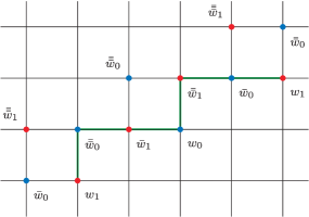
Figure 1: The labeling of lattice points in accordance with the prescribed periodicity and definition of $n=2m-l$.

In order for the constraint to define the iterates of $w_{0}$ and $w_{1}$ consistently, we require the equation defining the evolution at $(l,m)$ to coincide with the equation at $(l+4,m+2)$, hence, we require

$$p_{l+4}-q_{m+2}=p_{l}-q_{m},$$

which, by a separation of variables argument, defines a constant in $l$ and $m$, which we label $h$, given by

$$p_{l+4}-p_{l}=q_{m+2}-q_{m}:=h.$$

This difference equation defines $6$ additional constants. That is to say that the difference equation for $p_{l}$ is of degree $4$, defining $4$ constants in general, and the difference equation for $q_{m}$ is of degree $2$, defining $2$ new constants. We label these constants $a_{1},\ldots,a_{6}$, which enter the system via $q_{m}$ and $q_{l}$ by letting

$$q_{m}=\begin{cases}\dfrac{mh}{2}-a_{1}&\text{if}\ m=0\ \mathrm{mod}\,2,\vspace{1mm}\\ \dfrac{mh}{2}-a_{2}&\text{if}\ m=1\ \mathrm{mod}\,2,\end{cases}$$ (2.3)

$$p_{l}=\begin{cases}\dfrac{lh}{4}-a_{3}&\text{if}\ l=0\ \mathrm{mod}\,4,\vspace{1mm}\\ \dfrac{lh}{4}-a_{4}&\text{if}\ l=1\ \mathrm{mod}\,4,\vspace{1mm}\\ \dfrac{lh}{4}-a_{5}&\text{if}\ l=2\ \mathrm{mod}\,4,\vspace{1mm}\\ \dfrac{lh}{4}-a_{6}&\text{if}\ l=3\ \mathrm{mod}\,4.\end{cases}$$ (2.4)

The mapping that brings $n\to n+1$ is called the generating shift, as any shift on the lattice is some power of the generating shift. The generating shift is equivalent to the shift $(l,m)\to(l+1,m+1)$, hence, the mapping corresponding to $n\to n+1$ permutes the roles of the $a_{i}$ in the following way

$$\begin{pmatrix}\bar{a}_{1}&\bar{a}_{2}&\bar{a}_{3}\\ \bar{a}_{4}&\bar{a}_{5}&\bar{a}_{6}\end{pmatrix}=\begin{pmatrix}a_{2}+\dfrac{h}{2}&a_{1}-\dfrac{h}{2}&a_{4}+\dfrac{h}{4}\vspace{1mm}\\ a_{5}+\dfrac{h}{4}&a_{6}+\dfrac{h}{4}&a_{3}-\dfrac{3h}{4}\end{pmatrix}.$$ (2.5a)

In particular, notice that $$\bar{\bar{\bar{\bar{a}}}}_{i}=a_{i} l m 0 \mathrm{mod}\,4$$. If we assume and are , under this correspondence, the equations governing the lattice variables are

$$(\bar{w}_{0}-\bar{\bar{w}}_{0})(w_{1}-\bar{\bar{\bar{w}}}_{1})=a_{1}-a_{6}-\dfrac{nh}{4}-h,$$ (2.5b)

$$(\bar{w}_{1}-\bar{\bar{w}}_{1})(w_{0}-\bar{\bar{\bar{w}}}_{0})=a_{2}-a_{4}-\dfrac{nh}{4}.$$ (2.5c)

Let us simplify these equations by introducing variable $u$ and $v$ by

$$u=\bar{w}_{0}-w_{0},\qquad v=\bar{w}_{1}-w_{1},$$

hence, (2.5b) and (2.5c) become the degree 4 mapping

$$\bar{u}(v+\bar{v}+\bar{\bar{v}})=a_{1}-a_{6}-\dfrac{nh}{4}-h,$$ (2.6a)

$$\bar{v}(u+\bar{u}+\bar{\bar{u}})=a_{2}-a_{4}-\dfrac{nh}{4}.$$ (2.6b)

We use the second equation to obtain $v$ in terms of $u$ and its iterates, which then gives us an equation which may be written solely in terms of $\nu=\bar{u}/u$, reducing this fourth order system to a third order system

$$\dfrac{a_{1}-a_{5}-\frac{n+4}{h}}{1+\bar{\nu}+\bar{\nu}\bar{\bar{\nu}}}+\dfrac{\nu\left(a_{2}-a_{4}-\frac{nh}{4}\right)}{1+\nu+\nu\bar{\nu}}+\dfrac{\nu\underline{\nu}\left(a_{1}-a_{3}-\frac{nh}{4}\right)}{1+\underline{\nu}+\nu\underline{\nu}}=a_{1}-a_{6}-\dfrac{(n+4)h}{4}.$$

It is not completely trivial to see that this is a third order system with an invariant, $d_{1}$, which defines our second order evolution

$$\dfrac{\nu\underline{\nu}\left(a_{1}-a_{3}-\frac{nh}{4}\right)}{1+\underline{\nu}+\underline{\nu}\nu}-\dfrac{a_{2}-a_{4}-\frac{nh}{4}}{1+\nu+\nu\bar{\nu}}=d_{1}+a_{1}+a_{4}+a_{5}.$$ (2.7)

It is worth reminding the reader that we are primarily interested in the fourth power of this map, because the parameters change with each power of the map in accordance with (2.5a), in a similar manner to the asymmetric forms of discrete Painlevé equations provided by Kruskal et al. [23]. To avoid any confusion, we use a common notation to describe this map:

$$\left(\begin{array}[]{@{}c c c c}a_{1}&a_{2}&a_{3}&d_{1}\\ a_{4}&a_{5}&a_{6}&d_{2}\end{array};n,\underline{\nu},\nu\!\right)\to\left(\begin{array}[]{@{}c c c c}a_{2}+\dfrac{h}{2}&a_{1}-\dfrac{h}{2}&a_{4}+\dfrac{h}{4}&d_{1}\vspace{1mm}\\ a_{5}+\dfrac{h}{4}&a_{6}+\dfrac{h}{4}&a_{3}-\dfrac{3h}{4}&d_{2}\end{array};n+1,\nu,\overline{\nu}\!\right).$$

The fourth power of this mapping fixes the $a_{i}$ variables and sends $n$ to $n+4$.

We now describe a Lax pair for this system. A general method for determining the Lax representation of an autonomous reduction has been known for some time. While there were examples of derivations of Lax pairs for non-autonomous lattice equations [11, 12], a direct method for determining a Lax representation was presented only recently [37, 39]. One of the interesting consequences of this theory is that the resulting Lax matrices factorize in a novel manner.

The starting point for the Lax pair for the reduction is the Lax pair for the lattice equation. In this case, the Lax representation is given by

$$\Psi_{l+1,m}=L_{l,m}\Psi_{l,m},$$

$$\Psi_{l,m+1}=M_{l,m}\Psi_{l,m},$$

where

$$L_{l,m}=\begin{pmatrix}-w_{l+1,m}&1\\ -\kappa-w_{l,m}w_{l+1,m}+p_{l}&w_{l,m}\end{pmatrix},$$ (2.8a)

$$M_{l,m}=\begin{pmatrix}-w_{l,m+1}&1\\ -\kappa-w_{l,m}w_{l,m+1}+q_{m}&w_{l,m}\end{pmatrix},$$ (2.8b)

where $\kappa$ is a spectral parameter. The consistency of this system, in the calculation of $\Psi_{l+1,m+1}$, gives us the condition

$$L_{l,m+1}M_{l,m}=M_{l+1,m}L_{l,m},$$

which is equivalent to imposing (1.1).

We introduce a new non-autonomous spectral paramater, related to $\kappa$ by

$$x=\dfrac{lh}{4}-\kappa.$$ (2.9)

Using (2.2), (2.9), (2.3) and (2.4), we can represent linear problems in $l$, $m$ and $\kappa$ in terms of $x$, $n$ and the $a_{i}$ variables. Let us form two operators, $A_{n}(x)$ and $B_{n}(x)$, that are equivalent to the shifts $(l,m)\to(l+4,m+2)$ and $(l+1,m+1)$ respectively. This gives us a linear system satisfying the equations

$$Y_{n}(x+h)=A_{n}(x)Y_{n}(x),$$ (2.10a)

$$Y_{n+1}\left(x+\dfrac{h}{4}\right)=B_{n}(x)Y_{n}(x).$$ (2.10b)

These matrices are given by the products

$$A_{n}(x)\cong L_{l+3,m+2}L_{l+2,m+2}M_{l+2,m+1}L_{l+1,m+1}L_{l,m+1}M_{l,m},$$

$$B_{n}(x)\cong L_{l,m+1}M_{l,m}.$$

Explicitly, this is

$$B_{n}(x)=\begin{pmatrix}-\bar{w}_{1}&1\\ x-a_{3}-\bar{\bar{w}}_{0}\bar{w}_{1}&\bar{\bar{w}}_{2}\end{pmatrix}\begin{pmatrix}-\bar{\bar{w}}_{0}&1\\ x+\dfrac{nh}{4}-a_{1}-\bar{\bar{w}}_{0}w_{1}&w_{1}\end{pmatrix},$$

$$A_{n}(x)=\begin{pmatrix}-w_{1}&1\\ x-a_{6}-\bar{w}_{0}w_{1}&\bar{w}_{0}\end{pmatrix}\begin{pmatrix}-\bar{w}_{0}&1\\ x-a_{5}-\bar{w}_{0}\bar{\bar{w}}_{1}&\bar{\bar{w}}_{1}\end{pmatrix}$$

$$\hphantom{A_{n}(x)=}{}\times\begin{pmatrix}-\bar{\bar{w}}_{1}&1\\ x+\dfrac{nh}{4}-a_{2}-w_{0}\bar{\bar{w_{1}}}&w_{0}\end{pmatrix}\begin{pmatrix}-w_{0}&1\\ x-a_{4}-w_{0}\bar{w}_{1}&\bar{w}_{1}\end{pmatrix}B_{n}(x),$$ (2.11)

whose compatibility, given by

$$A_{n+1}\left(x+\dfrac{h}{4}\right)B_{n}(x)-B_{n}(x+h)A_{n}(x)\equiv 0,$$

gives (2.5). Through gauge transformations, we could express this in terms of the $u$ and $v$, or $\nu$, but we leave this out for succision.

3 Correspondence with d-P$\boldsymbol{\big{(}A_{2}^{(1)*}\big{)}}$

For very simple reductions, it is often straightforward to write down a correspondence between the variables on the lattice and the variables of the corresponding discrete Painlevé equation. For higher equations, the correspondences may be highly non-trivial and requires some auxiliary information as a guide. In the case of $q$-$\mathrm{P}\big{(}A_{2}^{(1)}\big{)}$, the auxiliary information was the Lax pair, which was found by Sakai [49] and Yamada [55]. Nicholas Witte and this author showed these two Lax pairs were related, furthermore that the associated linear problem for the special hypergeometric solutions may be expressible in terms of a certain orthogonal polynomial ensemble [53].

Our guide in this case is the Lax pair of Arinkin and Borodin [2]. While the result of Arinkin and Borodin was indeed of interest to many in the field, the Lax pair presented was not as explicitly presented as other Lax pairs in the literature (see for example [17, 25, 42]). We use this opportunity to present an explicit parameterization of this Lax pair.

Before doing so, we first examine some of the properties of the Lax pair we have thus far. The matrix $A_{n}(x)$ is of degree $3$, and may be written

$$A_{n}(x)=\mathcal{A}_{0,n}+\mathcal{A}_{1,n}x+\mathcal{A}_{2,n}x^{2}+\mathcal{A}_{3,n}x^{3},$$

where $\mathcal{A}_{3,n}=I$. The other property that is important is that, by taking the determinant of (2.11), we see that

$$\det A_{n}(x)=\left(x-a_{1}+\dfrac{nh}{4}\right)\left(x-a_{2}+\dfrac{nh}{4}\right)(x-a_{3})(x-a_{4})(x-a_{5})(x-a_{6}).$$ (3.1)

What is crucial to making the correspondence is $\mathcal{A}_{2,n}$, which is of the form

$$\mathcal{A}_{2,n}=\begin{pmatrix}d_{1}+\dfrac{nh}{4}&0\\ \rho_{21}&d_{2}+\dfrac{nh}{4}\end{pmatrix},$$

where the $d_{1}$ is defined by (2.7) and $d_{2}$ is determined by

$$d_{1}+d_{2}+a_{1}+a_{2}+a_{3}+a_{4}+a_{5}+a_{6}=0.$$ (3.2)

The additional variable, labeled $\rho_{12}$, is

$$\rho_{21}=\bar{u}^{2}v+\bar{u}\left(a_{3}-a_{1}+\frac{nh}{4}+uv\right)+u\left(a_{3}+a_{4}+a_{6}+d_{1}+\frac{nh}{4}\right)+\left(d_{1}-d_{2}\right)w_{0},$$

however, given that $\mathcal{A}_{2,n}$ is a lower triangular matrix, and that $\mathcal{A}_{3,n}=I$, we may transform our linear problem, $Y_{n}(x)$, by multiplication on the left by a simple lower triangular matrix so that $\mathcal{A}_{2,n}$ is may be taken to be diagonal, hence, $\mathcal{A}_{n}(x)$ takes the general form

$$A_{n}(x)=x^{3}I+\!\begin{pmatrix}\!\left(d_{1}\!+\!\dfrac{nh}{4}\right)((x-\alpha)(x-y)+z_{1})\!\!\!\!&\left(d_{1}\!+\!\dfrac{nh}{4}\right)\omega(x-y_{n})\\ \!\!\!\!\left(d_{2}\!+\!\dfrac{nh}{4}\right)\dfrac{(\delta x-\epsilon)}{\omega}&\left(d_{2}\!+\!\dfrac{nh}{4}\right)((x-\beta)(x-y)+z_{2})\!\end{pmatrix}\!,\!\!\!$$ (3.3)

where the function $\omega$ is related to the gauge freedom. The functions, $\alpha$, $\beta$, $\delta$ and $\epsilon$ are specified by conditions (3.2) and (3.1). There is also a relation between $z_{1}$ and $z_{2}$, which means that $z_{1}$ and $z_{2}$ may be written in terms of a single variable, $z$, chosen later to simplify the evolution equations.

In the interest of being explicit, we give expressions for these functions; we define the notation

$$\sum_{k=0}^{6}\mu_{i}x^{k}=\det A_{n}(x),$$

then the functions $\alpha$, $\beta$, $\gamma$ and $\delta$ are given, in terms of the $\mu_{i}$, as

$$\alpha=\frac{h^{2}n^{2}}{16\left(d_{1}-d_{2}\right)}+\frac{4\left(\left(d_{2}-d_{1}\right)\left(y^{2}-z_{2}\right)+\mu_{3}+\mu_{4}y\right)}{\left(d_{1}-d_{2}\right)\left(4d_{1}+nh\right)}$$

$$\hphantom{\alpha=}{}+\frac{nh\left(d_{1}+d_{2}-y\right)}{4\left(d_{1}-d_{2}\right)}-\frac{d_{1}\left(y-d_{2}\right)+\mu_{4}-2y^{2}+z_{1}+z_{2}}{d_{1}-d_{2}},$$ (3.4a)

$$\beta=\frac{h^{2}n^{2}}{16\left(d_{2}-d_{1}\right)}-\frac{4\left(\left(d_{1}-d_{2}\right)\left(y^{2}-z_{1}\right)+\mu_{3}+\mu_{4}y\right)}{\left(d_{1}-d_{2}\right)\left(4d_{2}+nh\right)}$$

$$\hphantom{\beta=}{}-\frac{nh\left(d_{1}+d_{2}-y\right)}{4\left(d_{1}-d_{2}\right)}+\frac{y\left(d_{2}-2y\right)-d_{1}d_{2}+\mu_{4}+z_{1}+z_{2}}{d_{1}-d_{2}},$$ (3.4b)

$$\delta=\alpha\beta-\frac{4\left(\mu_{0}+\mu_{1}y\right)}{\left(d_{1}-d_{2}\right)y^{2}\left(4d_{1}+nh\right)}+\frac{4\left(\mu_{0}+\mu_{1}y\right)}{\left(d_{1}-d_{2}\right)y^{2}\left(4d_{2}+nh\right)}$$

$$\hphantom{\delta=}{}-\frac{z_{1}z_{2}}{y^{2}}+y(\alpha+\beta)+z_{1}+z_{2},$$ (3.4c)

$$\epsilon=\frac{16\mu_{0}-\left(4d_{1}+nh\right)\left(4d_{2}+nh\right)\left(\alpha y+z_{1}\right)\left(\beta y+z_{2}\right)}{y\left(4d_{1}+nh\right)\left(4d_{2}+nh\right)}.$$ (3.4d)

The relationship between $z_{1}$ and $z_{2}$ is expressed as the determinant

$$\det A(y)=\left(y^{3}+z_{1}\left(d_{1}+\dfrac{nh}{4}\right)\right)\left(y^{3}+z_{2}\left(d_{2}+\dfrac{nh}{4}\right)\right),$$

which we specify by letting the $(1,1)$ and $(2,2)$ entries of $A_{n}(y_{n})$ be

$$y^{3}+z_{1}\left(d_{1}+\dfrac{nh}{4}\right)=\dfrac{\left(y-a_{3}\right)\left(y-a_{4}\right)\left(y-a_{5}\right)\left(y-a_{6}\right)}{z+y},$$ (3.5a)

$$y^{3}+z_{2}\left(d_{2}+\dfrac{nh}{4}\right)=(z+y)\left(y-a_{1}+\dfrac{nh}{4}\right)\left(y-a_{2}+\dfrac{nh}{4}\right).$$ (3.5b)

This specifies $z$ in a manner that simplifies the resulting evolution equations. The equations (3.3), (3.4) and (3.5) specify a parameterization of the Lax matrix described in the work of Arinkin and Borodin [2] (written as $\mathcal{A}(z)$ in [2]).

We are now in a better position to explicitly relate the system defined by (2.6) with (1.2). The variable $y$ in (1.2) is

$$y=v\bar{u}+a_{3}+uv-\frac{v\left(v\bar{u}+uv+a_{3}-a_{4}\right)\left(u\bar{v}-v\bar{u}-a_{3}+a_{5}\right)}{v\left(2u\bar{v}-a_{2}-a_{3}+a_{4}+a_{5}+\frac{nh}{4}\right)+\bar{v}\left(u\bar{v}-a_{2}+a_{5}+\frac{nh}{4}\right)-v^{2}\bar{u}},\!\!\!\!$$ (3.6)

and the variable $z$ in (1.2) is most succinctly expressed in terms of $y$ as

$$z+y=\frac{v\left(y-a_{4}\right)\left(y-a_{5}\right)\left(y-a_{6}\right)}{\left(y-a_{1}+\frac{nh}{4}\right)\left(v\left(u\bar{v}-a_{2}+\frac{hn}{4}+y\right)+\bar{v}\left(u\bar{v}-a_{2}+a_{5}+\frac{nh}{4}\right)\right)}.$$ (3.7)

With these variables, defined in terms of $u$ and $v$, we can verify that the $y$ and $z$ satisfy

$$(\bar{\bar{\bar{\bar{z}}}}+y)(y+z)=\dfrac{(y-a_{3})(y-a_{4})(y-a_{5})(y-a_{6})}{\left(y-a_{1}+\frac{nh}{4}\right)\left(y-a_{2}+\frac{nh}{4}\right)},$$ (3.8a)

$$(\bar{\bar{\bar{\bar{y}}}}+\bar{\bar{\bar{\bar{z}}}})(y+\bar{\bar{\bar{\bar{z}}}})$$

$$\qquad{}=\dfrac{(\bar{\bar{\bar{\bar{z}}}}+a_{3})(\bar{\bar{\bar{\bar{z}}}}+a_{4})(\bar{\bar{\bar{\bar{z}}}}+a_{5})(\bar{\bar{\bar{\bar{z}}}}+a_{6})}{\left(\bar{\bar{\bar{\bar{z}}}}-(d_{1}+a_{1}+a_{2})+\frac{nh}{4}\right)\left(\bar{\bar{\bar{\bar{z}}}}+(d_{1}+a_{3}+a_{4}+a_{5}+a_{6}+h)+\frac{nh}{4}\right)},$$ (3.8b)

which may be identified with (1.2) when $\delta=h$, $\tilde{f}=\bar{\bar{\bar{\bar{f}}}}$, $t=nh/4$ and

$$a_{7}=-d_{1}-a_{1}-a_{2},\qquad a_{8}=d_{1}+a_{3}+a_{4}+a_{5}+a_{6}+h.$$

The constraint, (1.3), is trivially satisfied by this choice. At this point, we note that it is somewhat remarkable that this choice, coupled with the definition of the evolution of $u$ and $v$, given by (2.6), are sufficient to check that (1.2) is satisfied. To actually derive (1.2), we require a little more work.

This is a system of linear difference equations admitting two fundamental solutions, $Y_{\infty}$ and $Y_{-\infty}$, which are analytic throughout the complex plane, except for possible poles to the left and right of the $a_{i}$ respectively. The solutions are asymptotically represented, á la Birkhoff [3], by expansions of the form

$$Y_{\pm\infty}(x)=x^{3x/h}e^{-3x/h}\left(I+\dfrac{Y_{1}}{x}+\dfrac{Y_{2}}{x^{2}}+\cdots\right)\mathrm{diag}\left(x^{\frac{n-6}{4}+\frac{d_{1}}{h}},x^{\frac{n-6}{4}+\frac{d_{2}}{h}}\right).$$

A more current exposition detailing the existence of a more general class of solutions were obtained by [43]. The connection matrix is defined by

$$P(x)=(Y_{\infty}(x))^{-1}Y_{-\infty}(x),$$

which is $h$-periodic in $x$ (i.e., $P(x+h)=P(x)$). Borodin specified a canonical group of transformations, specified by a general form

$$\tilde{Y}_{n}(x)=R_{n}(x)Y_{n}(x),$$

that preserves this matrix [5] which he used with Arinkin to formulate the original Lax pair in [2].

Since the shift $n\to n+1$ has an undesired non-trivial effect on the parameters, we need to consider a transformation that sends $n\to n+4$, which we label $B^{\prime}_{n}(x)$. A Lax matrix that represents the shift $(l,m)\to(l,m+2)$ may be given by

$$B^{\prime}_{n}(x)\cong M_{l,m+1}M_{l,m},$$ (3.9)

which, is of the general form

$$B^{\prime}_{n}(x)=\begin{pmatrix}x+r_{1}&r_{2}\vspace{1mm}\\ -\dfrac{\left(\frac{nh}{4}-a_{1}-r_{1}\right)\left(\frac{nh}{4}-a_{2}-r_{1}\right)}{r_{2}}&\dfrac{nh}{2}+x-a_{1}-a_{2}-r_{1}\end{pmatrix}.$$

This means that our new auxiliary linear equation is

$$Y_{n+4}(x)=B^{\prime}_{n}(x)Y_{n}(x),$$

where the new compatibility condition is

$$B^{\prime}_{n}(x+h)A_{n}(x)-A_{n+4}(x)B^{\prime}_{n}(x)\equiv 0.$$ (3.10)

One may derive the entries, $r_{1}$ and $r_{2}$, by performing the required change of variables, from $w_{0}$ and $w_{1}$ to functions in $y$ and $z$ to (3.9), however, it is much more convenient to use the (3.10) directly, to give

$$r_{1}=\frac{1}{h}\left(d_{1}+\frac{nh}{4}\right)(\tilde{\alpha}-\alpha+\tilde{y}-y+1)+\tilde{\alpha}+\tilde{y},$$

$$r_{2}=\frac{\left(d_{1}+\frac{nh}{4}\right)w-\left(d_{1}+\frac{nh}{4}+h\right)\tilde{w}}{d_{1}-d_{2}+h}.$$

Using the definition of $y$ and $z$, the evolution, and the expressions for $y$ and $z$ in terms of $w_{0}$ and $w_{1}$ recovers the expression for $B_{n}^{\prime}(x)$ in terms of $w_{0}$ and $w_{1}$. Using these values for $r_{1}$ and $r_{2}$ in (3.10) gives us (1.2), meaning that the expressions, (3.6) and (3.7), in terms of $u$ and $v$ solve (3.8).

4 Symmetries

The Bäcklund transformations of (1.2) form a realization of an affine Weyl group of type $E_{6}^{(1)}$ [47]. It is interesting and possible to explore how the Schlesinger transformations, such as those explored by Borodin [5], are tied to the concept of consistency around a cube [33]. That is, we seek to relate the Bäcklund transformations for lattice equation, defined by the multilinear function, (1.1), to the discrete isomonodromic (or connection preserving) deformations of Borodin [5].

Naturally, the connection preserving deformations form sub-groups of the full affine Weyl groups of symmetries. The $q$-analogues of connection preserving deformations appeared in the work of Jimbo and Sakai [17], and there have been but a few steps towards a general system of Schlesinger transformations that describe symmetries for the discrete Painlevé equations [35, 48].

The first set of symmetries we wish to describe is permutations on the set of parameters $\{a_{1},a_{2}\}$ and the permutations on the set $\{a_{3},a_{4},a_{5},a_{6}\}$. Let us first describe the symmetry $s_{34}$, which permutes $a_{3}$ and $a_{4}$, which we will generalize to provide the symmetry for the remaining symmetry group on the set of parameters. It is important to also note that these symmetries commute with the fourth power of the generating shift, not the generating shift itself.

Let us describe the symmetry $s_{34}$ as a map that sends the lattice variables, $w_{i}$ and their iterates, to $\hat{w}_{i}$. The path described in 1 assumes a certain labeling where, left to right, the parameters cycle through $a_{3}$ to $a_{6}$. The action of $s_{34}$ on the $w_{i}$ has a trivial effect on almost all the lattice variables except for $\bar{w}_{1}$, which is related to $\hat{\bar{w}}_{1}$ by a quad centered at $\bar{w}_{1}$ with variables $a_{3}$ and $a_{4}$ on the edges, as in Fig. 2.

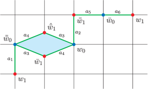
Figure 2: A pictorial representation of the symmetry $s_{34}$ which permutes the roles of $a_{3}$ and $a_{4}$.

That is to say that the symmetry is described by the equation

$$Q(\bar{\bar{w}}_{0},\bar{w}_{1},\hat{\bar{w}}_{1},w_{0},a_{4},a_{3})=0,$$

which means that the $s_{34}$ has the effect

$$s_{34}:\ \bar{w}_{1}\to\hat{\bar{w}}_{1}=\bar{w}_{1}+\dfrac{a_{3}-a_{4}}{w_{0}-\bar{\bar{w}}_{0}},\qquad s_{34}:\ a_{3}\to a_{4},\qquad s_{34}:\ a_{4}\to a_{3}.$$

This may be easily lifted to a symmetry of the $u$ and $v$ variables, where we note that the $u$ and $\bar{u}$ are unchanged, and the $v$ variables become

$$s_{34}:\ v\to\hat{v}=v+\dfrac{a_{3}-a_{4}}{u+\bar{u}},\qquad s_{34}:\ \bar{v}\to\hat{\bar{v}}=\bar{v}-\dfrac{a_{3}-a_{4}}{u+\bar{u}}.$$

This allows us to easily show that $\hat{y}=y$ and $\hat{z}=z$.

Similarly, to obtain the transformation, $s_{56}$, on the lattice variables, we place a quad centered at $\bar{w}_{0}$, which will permute $a_{5}$ and $a_{6}$ in the same way. That is to say that $s_{56}$ has a trivial effect on all the lattice variables except for $\bar{w}_{0}$, which is related to the transformed variable, $\hat{\bar{w}}_{0}$ via the relation

$$Q(\bar{\bar{w}}_{1},\hat{\bar{w}}_{0},\bar{w}_{0},w_{1},a_{5},a_{6})=0,$$

which means $s_{56}$ is specified by

$$s_{56}:\ \bar{w}_{0}\to\hat{\bar{w}}_{0}=\bar{w}_{0}+\dfrac{a_{5}-a_{6}}{w_{1}-\bar{\bar{w}}_{1}},\qquad s_{56}:\ a_{5}\to a_{6},\qquad s_{56}:\ a_{6}\to a_{5}.$$

We lift this to the variables $u$ and $v$ to give a trivial effect on $v$ and an action on $u$ and $\bar{u}$ described by

$$s_{56}:\ u\to\hat{u}=u+\dfrac{a_{5}-a_{6}}{v+\bar{v}},\qquad s_{56}:\ \bar{u}\to\hat{\bar{u}}=\bar{u}-\dfrac{a_{5}-a_{6}}{v+\bar{v}},$$

while, once again, this change has a trivial effect on $y$ and $z$.

To extrapolate this principle to obtain $s_{12}$ and $s_{45}$, we remark that the while the path chosen above gives us natural places to insert quads that permute the parameters, the path chosen is still arbitrary. That is to say that because $Q$ is multilinear, specifying the six initial conditions on any path is in one-to-one correspondence with the specification of variables along any other path. In this sense, while the standard staircase of [41, 51] is useful in describing the particular form of the evolution equations, (2.5), it is not actually that important in building a correspondence between (2.5) or (2.6) with (1.2). With this in mind, let us consider a small deviation of our original path that passes through $\underline{w}_{1}$ instead of $\bar{\bar{w}}_{1}$, as depicted in Fig. 3.

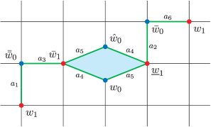
Figure 3: A pictorial representation of the symmetry $s_{45}$ which permutes the roles of $a_{4}$ and $a_{5}$.

The quad centered at $w_{0}$ in Fig. 3 has a trivial effect on each of the variables except for $w_{0}$. Knowing $\hat{w}_{0}$ and $\hat{\underline{w}}_{1}=\underline{w}_{1}$ is sufficient to obtain $\hat{\bar{\bar{w}}}_{1}$, i.e., one can recover the transformation of the variables along our original path by using the quad equation. This gives us that the symmetry that permutes the $a_{4}$ and $a_{5}$ is trivial for all variables except for $w_{0}$ and $\bar{\bar{w}}_{1}$, which is related to the transformed variables by the two quad equations

$$Q(\bar{w}_{1},\hat{w}_{0},w_{0},\underline{w}_{1},a_{5},a_{4})=0,\qquad Q\left(\hat{w}_{0},\underline{w}_{1},\hat{\bar{\bar{w}}}_{1},\bar{w}_{0},a_{2}-\frac{nh}{4},a_{4}\right)=0,$$

where the $nh/4$ contribution comes from the difference between an $p_{l}$ and a $q_{m}$ and $\underline{w}_{1}$ is known from knowledge of the original initial conditions, which gives us

$$s_{45}:\ w_{0}\to\hat{w}_{0}=w_{0}+\frac{\left(a_{4}-a_{5}\right)\left(w_{0}-\bar{w}_{0}\right)}{a_{5}-a_{2}+\frac{nh}{4}+\left(w_{0}-\bar{w}_{0}\right)\left(\bar{w}_{1}-\bar{\bar{w}}_{1}\right)},$$

$$s_{45}:\ \bar{w}_{1}\to\hat{\bar{w}}_{1}=\bar{w}_{1}+\dfrac{(w_{0}-\bar{w}_{0})(\bar{w}_{1}-\bar{\bar{w}}_{1})}{\bar{w}_{0}-\hat{w}_{0}},\qquad s_{45}:\ a_{4}\to a_{5},\qquad s_{45}:\ a_{5}\to a_{4}.$$

The transformation fixes $\bar{u}$ and $v$, and changes $u$ and $\bar{v}$ in the following manner,

$$s_{45}:\ u\to\hat{u}=u+\dfrac{u(a_{4}-a_{5})}{\frac{nh}{4}+u\bar{v}-a_{2}+a_{5}},\qquad s_{45}:\ \bar{v}\to\hat{\bar{v}}=\bar{v}+\dfrac{\bar{v}(a_{4}-a_{5})}{\frac{nh}{4}+u\bar{v}-a_{2}+a_{4}},$$

which also has a trivial effect on $y$ and $z$.

To obtain the transformation that permutes the $a_{1}$ and $a_{2}$ variables, the simplest choice of path passes through $\tilde{w}_{1}$ (i.e., $w_{1}(n+4)$) and $\bar{\bar{\bar{w}}}_{3}$. By placing a quad centered at $\bar{\bar{w}}_{0}$, the transformation fixes all the variables, except for $\bar{\bar{w}}_{0}$ on this path, meaning the transformation, changes $w_{0}$, $\bar{w}_{1}$ and $\bar{\bar{w}}_{1}$ in accordance with

$$Q\left(w_{1},\bar{\bar{w}}_{0},\hat{\bar{\bar{w}}}_{0},\tilde{w}_{1},a_{2},a_{1}\right)=0,\qquad Q\left(\hat{\bar{\bar{w}}}_{0},\hat{\bar{w}}_{1},\tilde{w}_{1},\bar{\bar{\bar{w}}}_{0},a_{1}-\frac{nh}{4},a_{3}\right)=0,$$

$$Q\left(\hat{\bar{w}}_{1},\bar{\bar{\bar{w}}}_{0},\hat{w}_{1},\hat{w}_{0},a_{1}-\frac{nh}{4},a_{4}\right)=0,$$

which we will write implicitly as

$$s_{12}:\ \bar{\bar{w}}_{0}\to\hat{\bar{\bar{w}}}_{0}=\bar{\bar{w}}_{0}+\dfrac{a_{2}-a_{1}}{\tilde{w}_{1}-w_{1}},\qquad s_{12}:\ \bar{w}_{1}\to\hat{\bar{w}}_{1}=\tilde{w}_{1}+\dfrac{\frac{nh}{4}-a_{1}+a_{3}}{\bar{\bar{\bar{w}}}_{0}-\hat{\bar{\bar{w}}}_{0}},$$

$$s_{12}:\ w_{0}\to\hat{w}_{0}=\bar{\bar{\bar{w}}}_{0}+\dfrac{\frac{nh}{4}-a_{1}+a_{4}}{\bar{\bar{w}}_{1}-\hat{\bar{w}}_{1}},\qquad s_{12}:\ a_{1}\to a_{2},\qquad s_{12}:\ a_{2}\to a_{1},$$

which again, may be expressed in terms of transformations in $u$ and $v$ as

$$s_{12}:\ u\to\hat{u}=u_{n}+\dfrac{\frac{nh}{4}-a_{2}+a_{4}}{\bar{v}}-\dfrac{\frac{nh}{4}-a_{1}+a_{4}}{\hat{\bar{v}}},\qquad s_{12}:\ v\to\hat{v}=v+\lambda,$$

$$s_{12}:\ \bar{u}\to\hat{\bar{u}}=\bar{u}+\dfrac{\frac{nh}{4}-a_{1}+a_{3}}{v}-\dfrac{\frac{nh}{4}-a_{2}+a_{3}}{\hat{v}},\qquad s_{12}:\ v\to\hat{\bar{v}}=\bar{v}-\lambda,$$

where

$$\lambda=\frac{\left(a_{1}-a_{2}\right)v\bar{v}}{v\left(\left(\bar{u}+u\right)\bar{v}-a_{2}+a_{4}+\frac{nh}{4}\right)+\bar{v}\left(a_{3}-a_{1}+\frac{nh}{4}\right)}.$$

This transformation has a trivial effect on $d_{1}$, $d_{2}$, $y$ and $z$.

Let us now describe two transformations, $T_{a_{1}}$ and $T_{a_{3}}$, which, in combination with the symmetries described above, will be sufficient to describe a complete set of connection preserving deformations described by Borodin [5]. These transformations will necessarily act non-trivially on the variable $y$ and $z$ and may be used to obtain infinite families of rational and Riccati solutions from the seed solutions in Section 5.

The first transformation, $T_{a_{1}}$, may be considered to be the image of the shift in the positive $m$ direction. This may also be seen to be induced by a lift of the $M_{l,m}$ matrix, (2.8b), to the level of the reduction. This also represents the discrete analogue of a fundamental Schlesinger transformation in the work of Jimbo and Miwa [16] since (2.8b) induces the transformation of the linear system

$$\hat{Y}_{n}(x)=R_{n,a_{1}}(x)Y_{n}(x),$$ (4.1)

where $R_{n,a_{1}}(x)$ is linear in $x$ and

$$\det R_{n,a_{1}}(x)=x-a_{1}-\frac{nh}{4}.$$

This transformation may be described on the level of the lattice variables by

$$T_{a_{1}}:\ w_{1}\to\hat{w}_{1}=\bar{\bar{w}}_{0},\qquad T_{a_{1}}:\ w_{0}\to\hat{w}_{0}=\bar{\bar{w}}_{1},$$

$$Q\left(\bar{w}_{1},w_{0},\hat{\bar{w}}_{1},\bar{\bar{w}}_{1},a_{2}-\frac{nh}{4},a_{4}\right)=0,\qquad Q\left(\bar{w}_{0},w_{1},\hat{\bar{w}}_{0},\bar{\bar{w}}_{1},a_{1}+h-\frac{nh}{4},a_{5}\right)=0,$$

$$Q\left(\bar{\bar{w}}_{0},\bar{w}_{1},\hat{\bar{\bar{w}}}_{0},\hat{\bar{w}}_{1},a_{2}-\frac{nh}{4},a_{3}\right)=0,\qquad Q\left(\bar{\bar{w}}_{1},\bar{w}_{0},\hat{\bar{\bar{w}}}_{1},\hat{\bar{w}}_{0},a_{1}+h-\frac{nh}{4},a_{6}\right)=0,$$

where the parameters, $a_{1}$ and $a_{2}$ change via the rule

$$T_{a_{1}}:\ a_{1}\to a_{2},\qquad T_{a_{1}}:\ a_{2}\to a_{1}-h.$$

When lifted to the level of the $u$ and $v$ variables, the transformation is described by

$$T_{a_{1}}:\ u\to\hat{u}=-v-\bar{v}-\dfrac{\frac{h(n+4)}{4}-a_{1}+a_{6}}{\bar{u}},$$

$$T_{a_{1}}:\ v\to\hat{v}=-u-\bar{u}-\dfrac{\frac{nh}{4}-a_{2}+a_{4}}{\bar{v}},$$

$$T_{a_{1}}:\ \bar{u}\to\hat{\bar{u}}=v+\dfrac{\frac{h(n+4)}{4}-a_{1}+a_{6}}{\bar{u}}-\dfrac{\frac{nh}{4}-a_{2}+a_{3}}{\hat{\bar{v}}},$$

$$T_{a_{1}}:\ \bar{v}\to\hat{\bar{v}}=u-\dfrac{\frac{h(n+4)}{4}-a_{1}+a_{5}}{\hat{u}}+\dfrac{\frac{nh}{4}-a_{2}+a_{4}}{\bar{v}},$$

which is equivalent to a double shift in $n$. The first implication of this is that our invariant, $d_{1}$ and $d_{2}$ change, in accordance with the rule

$$T_{a_{1}}:\ d_{1}\to d_{2},\qquad T_{a_{1}}:\ d_{2}\to d_{1}+h.$$

To calculate the effect of $T_{a_{1}}$ on $y$ and $z$, we use the compatibility between (4.1) and (2.10a), where $A_{n}(x)$ is defined by (3.3). The effects of $T_{a_{1}}$ on $y$ and $z$ are given by

$$T_{a_{1}}:\ y\to\hat{y}=y+\dfrac{1}{d_{1}-d_{2}}\left(y^{2}+\frac{\delta\left(d_{1}+\frac{nh}{4}\right)\left(d_{2}+\frac{nh}{4}\right)}{\left(d_{1}+\frac{nh}{4}\right)\left(\alpha-a_{1}+\frac{nh}{4}\right)-\frac{\left(\frac{nh}{4}-a_{1}\right)^{3}-z_{1}\left(d_{1}+\frac{nh}{4}\right)}{y-a_{1}+\frac{nh}{4}}}\right.$$

$$\left.\qquad{}-\frac{z_{1}\left(d_{1}+\frac{nh}{4}\right)+y^{3}}{y-a_{1}+\frac{nh}{4}}+a_{1}\left(d_{2}+a_{1}-\frac{nh}{4}+y\right)-d_{2}\left(\beta+\frac{nh}{4}\right)-\frac{(\beta+y)nh}{4}\right),$$

$$T_{a_{1}}:\ z\to\hat{z},$$

where the relation between $z$ and $\hat{z}$ is given implicitly by the relation

$$\hat{z}_{1}=\dfrac{y-\hat{y}}{d_{2}+\frac{nh}{4}}\left(d_{1}\left(\alpha-a_{1}+\frac{nh}{4}\right)-\frac{a_{1}nh}{4}+\left(\beta-\hat{y}\right)\left(d_{2}+\frac{nh}{4}\right)+\frac{h^{2}n^{2}}{16}+\frac{\alpha nh}{4}\right.$$

$$\left.\hphantom{\hat{z}_{1}=}{}-\frac{\left(\frac{nh}{4}-a_{1}\right){}^{3}-z_{1}\left(d_{1}+\frac{nh}{4}\right)}{\left(-a_{1}+\frac{nh}{4}+y\right)}+\frac{z_{2}\left(d_{2}+\frac{nh}{4}\right)}{\left(y-\hat{y}\right)}\right).$$

Similarly, if we were to lift the $L_{l,m}$ to the reduced linear problem, we obtain a linear system

$$\hat{Y}_{n}(x)=R_{n,a_{3}}(x)Y_{n}(x),$$ (4.2)

where $R_{n,a_{3}}(x)$ is also linear in $x$ and

$$\det R_{n,a_{3}}(x)=x-a_{3}.$$

This is a fundamental Schlesinger transformation that induces a transformation, which we label $T_{a_{3}}$, that has the effect of fixing $a_{1}$ and $a_{2}$, permuting the other variables, $a_{3}$ to $a_{6}$, as follows

$$T_{a_{3}}:\ a_{3}\to a_{4},\qquad T_{a_{3}}:\ a_{4}\to a_{5},\qquad T_{a_{3}}:\ a_{5}\to a_{6},\qquad T_{a_{3}}:\ a_{6}\to a_{3}-h.$$

The effect on the lattice variable is given in terms of the multilinear function, $Q$, as

$$T_{a_{3}}:\ \bar{w}_{0}\to\hat{\bar{w}}_{0}=w_{1},\qquad T_{a_{3}}:\ \bar{w}_{1}\to\hat{\bar{w}}_{1}=w_{0},$$

$$T_{a_{3}}:\ \bar{\bar{w}}_{0}\to\hat{\bar{\bar{w}}}_{0}=\bar{w}_{1},\qquad T_{a_{3}}:\bar{\bar{w}}_{0}\to\hat{\bar{\bar{w}}}_{1}=\bar{w}_{0},$$

$$Q\left(w_{1},\hat{w}_{1},\bar{\bar{w}}_{0},\bar{w}_{1},a_{3},a_{1}-\frac{nh}{4}\right)=0,\qquad Q\left(w_{0},\hat{w}_{0},\bar{\bar{w}}_{1},\bar{w}_{0},a_{5},a_{2}-\frac{nh}{4}\right)=0.$$

The effect of $T_{a_{3}}$ on $u$ and $v$ is simply given by the inverse of (2.6). In the same way as for $T_{a_{1}}$, we use (4.2), (2.10a) and (3.3) to find that

$$T_{a_{3}}:\ d_{1}\to d_{2},\qquad T_{a_{3}}:\ d_{2}\to d_{1}+h,$$

and the effect on $y$ and $z$ is given by

$$T_{a_{3}}:\ y\to\hat{y}=y+\dfrac{1}{d_{1}-d_{2}}\left(\frac{z_{1}\left(d_{1}+\frac{nh}{4}\right)+y^{3}}{\left(a_{3}-y\right)}+y^{2}-\beta d_{2}+a_{3}\left(d_{2}+\frac{nh}{4}+y\right)\right.$$

$$\left.\qquad{}-\frac{\beta nh}{4}+a_{3}^{2}+\frac{\delta\left(y-a_{3}\right)\left(d_{1}+\frac{nh}{4}\right)\left(d_{2}+\frac{nh}{4}\right)}{\left(\left(d_{1}+\frac{nh}{4}\right)\left(y\left(\alpha-a_{3}\right)-\alpha a_{3}+z_{1}\right)+a_{3}^{2}\left(a_{3}+d_{1}+\frac{nh}{4}\right)\right)}\right),$$

$$T_{a_{3}}:\ z\to\hat{z},$$

where we give the relation implicitly by stating that $\hat{z}_{1}$ is specified by

$$\hat{z}_{1}=\dfrac{y-\hat{y}}{d_{2}+\frac{nh}{4}}\left(\frac{z_{1}\left(d_{1}+\frac{nh}{4}\right)+y^{3}}{\left(y-a_{3}\right)\left(d_{2}+\frac{nh}{4}\right)}-\frac{a_{3}\left(d_{1}+\frac{nh}{4}+y\right)}{d_{2}+\frac{nh}{4}}-\frac{a_{3}^{2}}{d_{2}+\frac{nh}{4}}+\beta\right.$$

$$\left.\hphantom{\hat{z}_{1}=}{}+\frac{\alpha\left(d_{1}+\frac{nh}{4}\right)-y^{2}}{d_{2}+\frac{nh}{4}}+\frac{z_{2}}{y-\hat{y}}-\hat{y}\right).$$

What is important in these calculations is that the general symmetry structure of reductions of quad-equations apparent. In fact, the way in which the general symmetry structure is described by quad-equations is much more natural as a higher-dimensional reduction than a two-dimensional reduction. In this case, this is more naturally a 6-dimensional reduction. This work, in combination with [39], is sufficient to give a symmetry structure to reductions that are equivalent to all the systems below those with $A_{2}^{(1)}$ surfaces in the Sakai classification [47].

It should be noted that the above constitutes a set of symmetries that have been derived by an application of $Q$ as a symmetry. There are other equations that are consistent with $Q$, which can be found in the work of Boll [4], however, none of the tested equations that are consistent with (1.1) seemed to produce a non-trivial transformation of the Painlevé variables, $y$ and $z$. Perhaps some further investigation is required in this direction.

5 Special solutions

Lastly, this brings us to the method we wish to use to solve (1.2). There are numerous studies that show that the Painlevé equations admit solutions expressible in terms of hypergeometric and confluent hypergeometric functions (see [34] for a review). Many of the simplest discrete Riccati solutions were, including those for (1.2), were presented in [46]. A more geometric approach was taken for the $q$-Painlevé equations by Kajiwara et al. [21]. The work of Nicholas Witte has shown that is possible to find many hypergeometric solutions, including those for (1.2), in terms of the moments of a certain semi-classically deformed orthogonal polynomial ensembles [52], which is closely related to the Padé approximation method of Yamada et al. [54].

For an equation such as (1.2), it is not immediately obvious how to even obtain very basic rational solutions. Our work on the reduction gives us a number of different equivalent forms of the equation that we may solve explicitly. If we take (2.6) in the special case in which the parameters of the lattice equation, $p_{l}$ and $q_{m}$, are linear

$$p_{l}=a+\dfrac{hl}{4},\qquad q_{m}=b+\dfrac{hm}{2},$$

corresponding to the choice of parameters

$$a_{1}=-b,\quad a_{2}=-b-\frac{h}{2},\quad a_{3}=-a,\quad a_{4}=-a-\frac{h}{4},\quad a_{5}=-a-\frac{h}{2},\quad a_{6}=-a-\frac{3h}{4},$$

the evolution equations simplify to

$$\bar{v}(u+\bar{u}+\bar{\bar{u}})=a-b-\dfrac{(n+1)h}{4},\qquad\bar{u}(v+\bar{v}+\bar{\bar{v}})=a-b-\dfrac{(n+1)h}{4}.$$

If $u=v$, this becomes a version of d-$\mathrm{P}_{\rm I}$ that has no rational solutions. This equation does possess a relatively simple one parameter family of rational solutions, in the case that $u$ is constant and $v$ is linear, explicitly we have

$$u=\dfrac{1}{3\lambda},\qquad v=\lambda\left(a-b+\frac{nh}{4}\right),$$

or equivalently, this choice prescribes a two parameter family of solutions to the system in $w_{0}$ and $w_{1}$, given by

$$w_{0}=\dfrac{n}{3\lambda}+\theta_{1},\qquad w_{1}=\lambda n\left(a-b+\frac{h}{8}\right)+\dfrac{\lambda n^{2}h}{8}+\theta_{2},$$

where $\theta_{1}$ and $\theta_{2}$ are arbitrary constants. Substituting these solutions into $y$, $z$, $d_{1}$ and $d_{2}$ gives

$$d_{1}=2a+b+\dfrac{5h}{6},\qquad d_{1}=2a+b+\dfrac{7h}{6},$$

$$y=\frac{1}{24}\bigg{(}\frac{7h^{2}(2nh-h-8a+8b)}{64a^{2}-16a(8b+h(2n-1))+64b^{2}+16bh(2n-1)+h^{2}(4(n-1)n-1)}$$

$$\hphantom{y=}{}-8a-16b-4hn-7h\bigg{)},$$

$$z=\frac{1}{24}\left(h\left(\frac{14h}{-8a+8b+2nh-5h}-4n+19\right)+40a-16b\right).$$

Alternatively, by swapping the roles of $u$ and $v$ we obtain the solution

$$d_{1}=2a+b+\dfrac{2h}{3},\qquad d_{2}=d_{2}=2a+b+\dfrac{4h}{3},$$

$$y=\frac{1}{24}\left(h\left(-\frac{5h}{8a-8b-2nh+h}-4n-7\right)-8a-16b\right),$$

$$z=\frac{1}{24}(40a-16b+h(19-4n)).$$

To consider the hypergeometric solutions, let us first review the work of Ramani et al. [46] who present solutions of the form

$$\tilde{y}=\dfrac{\sigma_{1}\tilde{z}+\sigma_{2}}{\sigma_{3}\tilde{z}+\sigma_{4}},\qquad\tilde{z}=\dfrac{\tau_{1}y+\tau_{2}}{\tau_{3}z+\tau_{4}},$$

where the $\sigma_{i}$’s and $\tau_{i}$’s are functions on $n$ alone. There are a multitude of values the $\sigma$ and $\tau$ variables may take in order for the evolution to coincide with (1.2). We choose just one, which yields

$$\tilde{y}=\frac{\tilde{z}\left(a_{2}-\frac{1}{4}h(n+4)\right)+a_{3}a_{4}}{\tilde{z}-a_{2}+a_{3}+a_{4}+\frac{hn}{4}+h},\qquad\tilde{z}=\frac{-y\left(a_{6}+\frac{nh}{4}\right)+a_{1}y+a_{5}\left(a_{6}-y\right)}{y-a_{1}+\frac{nh}{4}},$$

where we have one of two alternative constraints, either

$$d_{1}+a_{1}+a_{3}+a_{4}+h=0\qquad\textrm{or}\qquad d_{1}+a_{2}+a_{3}+a_{4}+h=0.$$

Combining these two equations gives us a single second order difference equation which also admits the hypergeometric differential equation in a continuum limit [46]. These solutions may be identified as hypergeometric functions by relating these recurrence relations to contiguous relations for hypergeometric functions of type ${}_{3}F_{2}(1)$, as done by Kajiwara [18].

We can now consider the possibility of the evolution of $\nu$ coinciding with a fractional linear transformation of the form

$$\bar{\nu}=\dfrac{c_{11}\nu+c_{12}}{c_{21}\nu+c_{22}},$$ (5.1)

which may be inverted so calculate $\underline{\nu}$ in terms of $\nu$. Substituting (5.1), and its inverse, into (2.7) gives us a number of conditions in the variable $\nu$, which we solve to give the equation

$$\bar{\nu}=\dfrac{(1+\nu)\left(\dfrac{nh}{4}+d_{1}+a_{3}+a_{4}+a_{5}\right)}{a_{2}-a_{4}-\dfrac{nh}{4}-\nu\left(\dfrac{nh}{4}+d_{1}+a_{3}+a_{4}+a_{5}\right)},$$

which coincides with the evolution of (2.7) so long as

$$2d_{1}+a_{1}+a_{2}+a_{3}+a_{4}+a_{5}+a_{6}=0.$$

In the language of the affine Weyl symmetries, this condition ensures that the parameters correspond to a point on a wall of an affine Weyl chamber.

To obtain the corresponding solution for $y$ and $z$, we first take the fourth power of this mapping to find $\tilde{nu}$ is given by

$$\tilde{\nu}=\dfrac{C_{11}\nu+C_{12}}{C_{21}\nu+C_{22}},$$

where

$$C_{11}=\left(\dfrac{nh}{2}-a_{1}-a_{2}+a_{3}+a_{4}+a_{5}-a_{6}\right)\left(\dfrac{h(n+4)}{2}-a_{1}-a_{2}+a_{3}+a_{4}-a_{5}+a_{6}\right),$$

$$C_{12}=-\left(2h-a_{1}+a_{2}-a_{3}-a_{4}+a_{5}+a_{6}\right)\left(\dfrac{h(n+4)}{2}-a_{1}-a_{2}+a_{3}+a_{4}-a_{5}+a_{6}\right),$$

$$C_{21}=\left(a_{1}-a_{2}-a_{3}-a_{4}+a_{5}+a_{6}\right)\left(\dfrac{nh}{2}-a_{1}-a_{2}+a_{3}+a_{4}+a_{5}-a_{6}\right),$$

$$C_{22}=\frac{h^{2}(n+4)^{2}}{4}-nh\left(a_{1}+a_{2}-a_{5}-a_{6}\right)+2\left(a_{3}h+a_{4}h+a_{5}h+a_{6}\left(a_{3}+a_{4}+h\right)\right.$$

$$\left.\hphantom{C_{22}=}{}-a_{2}\left(a_{5}+a_{6}+h\right)-a_{1}\left(a_{5}+a_{6}+3h\right)+a_{1}^{2}+a_{2}^{2}-a_{3}^{2}-a_{4}^{2}+a_{3}a_{5}+a_{4}a_{5}\right).$$

The constraint seems characteristically different from the solutions above, which means this is a hypergeometric solution for a different choice of parameters. We do not know how these two solutions are related.

Using the group of symmetries derived in Section 4 one is able to generate an infinite number of hypergeometric solutions, however, we do note that the one cannot apply the full set of Bäcklund transformations to the hypergeometric solutions. One characterization of the hypergeometric solutions is that they are solutions that are singular on a translational Bäcklund transformation. That is to say that these solutions are not just on a wall of the affine Weyl chamber, but they are on a barrier which one cannot pass through using Bäcklund transformations.

It would be interesting to consider determinantal structures, either from a bilinear approach [19] or an orthogonal polynomial approach [40]. Determinantal formulations are beyond the scope of this paper.

6 Conclusion

We have provided a reduction from one of the most degenerate lattice equations to an equation that sits above the sixth Painlevé equation in Sakai’s classification. While these reductions are somewhat complicated, their very existence suggests that the solutions to all the additive Painlevé equations, and many higher-dimensional additive equations, may be expressed in terms of the solutions of the lattice potential Korteweg–de Vries equation. A similar statement could be made about multiplicative type equations and the discrete Schwarzian Korteweg–de Vries equation. Furthermore, while we know of a reduction from the Schwarzian Korteweg–de Vries equation to the sixth Painlevé equation [28, 29], we believe there may exist a more complicated reduction from the Korteweg–de Vries equation to the sixth Painlevé equation that is yet to be found.

There is still a sense in which these reductions may be more naturally approached from a geometric perspective, where one is interested in mapping between biquadratic curves for the lattice equations and the (moving) biquadratics for the (non-autonomous) reductions. While this work suggests that the symmetries are most naturally viewed in terms of quad-equations on higher-dimensional lattices, Doliwa notes in [8] that it might be more natural to consider reductions from higher-dimensional lattice equations.

There are still also issues regarding the definitions and framework of connection preserving deformations. These connection preserving deformations should manifest themselves as automorphisms of the Galois group associated with the system of difference equations. This could present a natural extension of the connection preserving deformations that could be large enough to describe the full affine Weyl group of Bäcklund transformations, rather than just a restriction to the translational elements of the affine Weyl group.

This work on the symmetries of reduced equations applies a wide class of periodic reductions that have appeared in the literature. It is not entirely clear at this point how, or even whether, this procedure may be applied to the so-called twisted reductions explored by recent work [13, 38]. This work suggests that the symmetry group of a $(s_{1},s_{2})$-reduction is at least a lattice of dimension $s_{1}+s_{2}$, hence, we suspect it would take a $(4,4)$-reduction of Q4 to be able to be identified with the full parameter version of the elliptic Painlevé equation.

Acknowledgements

This research is supported by Australian Research Council Discovery Grant #DP110100077.

References

- [1] Ablowitz M.J., Segur H., Exact linearization of a Painlevé transcendent, Phys. Rev. Lett. 38 (1977), 1103–1106.
- [2] Arinkin D., Borodin A., Moduli spaces of -connections and difference Painlevé equations, Duke Math. J. 134 (2006), 515–556, math.AG/0411584.
- [3] Birkhoff G.D., General theory of linear difference equations, Trans. Amer. Math. Soc. 12 (1911), 243–284.
- [4] Boll R., Classification of 3D consistent quad-equations, J. Nonlinear Math. Phys. 18 (2011), 337–365, arXiv:1009.4007.
- [5] Borodin A., Isomonodromy transformations of linear systems of difference equations, Ann. of Math. 160 (2004), 1141–1182, math.CA/0209144.
- [6] Clarkson P.A., Painlevé equations – nonlinear special functions, in Orthogonal Polynomials and Special Functions, Lecture Notes in Math., Vol. 1883, Springer, Berlin, 2006, 331–411.
- [7] Clarkson P.A., Kruskal M.D., New similarity reductions of the Boussinesq equation, J. Math. Phys. 30 (1989), 2201–2213.
- [8] Doliwa A., Non-commutative lattice-modified Gel’fand–Dikii systems, J. Phys. A: Math. Theor. 46 (2013), 205202, 14 pages, arXiv:1302.5594.
- [9] Dzhamay A., Sakai H., Takenawa T., Discrete Hamiltonian structure of Schlesinger transformations, arXiv:1302.2972.
- [10] Flaschka H., Newell A.C., Monodromy- and spectrum-preserving deformations. I, Comm. Math. Phys. 76 (1980), 65–116.
- [11] Hay M., Hierarchies of nonlinear integrable -difference equations from series of Lax pairs, J. Phys. A: Math. Theor. 40 (2007), 10457–10471.
- [12] Hay M., Hietarinta J., Joshi N., Nijhoff F.W., A Lax pair for a lattice modified KdV equation, reductions to -Painlevé equations and associated Lax pairs, J. Phys. A: Math. Theor. 40 (2007), F61–F73.
- [13] Hay M., Howes P., Shi Y., A systematic approach to reductions of type-Q ABS equations, arXiv:1307.3390.
- [14] Hay M., Kajiwara K., Masuda T., Bilinearization and special solutions to the discrete Schwarzian KdV equation, J. Math-for-Ind. 3A (2011), 53–62, arXiv:1102.1829.
- [15] Hone A.N.W., van der Kamp P.H., Quispel G.R.W., Tran D.T., Integrability of reductions of the discrete Korteweg–de Vries and potential Korteweg–de Vries equations, Proc. R. Soc. Lond. Ser. A Math. Phys. Eng. Sci. 469 (2013), 20120747, 23 pages, arXiv:1211.6958.
- [16] Jimbo M., Miwa T., Monodromy preserving deformation of linear ordinary differential equations with rational coefficients. II, Phys. D 2 (1981), 407–448.
- [17] Jimbo M., Sakai H., A -analog of the sixth Painlevé equation, Lett. Math. Phys. 38 (1996), 145–154, chao-dyn/9507010.
- [18] Kajiwara K., The hypergeometric solutions of the additive Painlevé equations with -type affine Weyl symmetry, Reports of RIAM Symposium No. 19ME-S2 (in Japanese).
- [19] Kajiwara K., Kimura K., On a -difference Painlevé III equation. I. Derivation, symmetry and Riccati type solutions, J. Nonlinear Math. Phys. 10 (2003), 86–102, nlin.SI/0205019.
- [20] Kajiwara K., Masuda T., Noumi M., Ohta Y., Yamada Y., solution to the elliptic Painlevé equation, J. Phys. A: Math. Gen. 36 (2003), L263–L272, nlin.SI/0303032.
- [21] Kajiwara K., Masuda T., Noumi M., Ohta Y., Yamada Y., Construction of hypergeometric solutions to the -Painlevé equations, Int. Math. Res. Not. 2005 (2005), 1441–1463, nlin.SI/0501051.
- [22] Kajiwara K., Noumi M., Yamada Y., A study on the fourth -Painlevé equation, J. Phys. A: Math. Gen. 34 (2001), 8563–8581, nlin.SI/0012063.
- [23] Kruskal M.D., Tamizhmani K.M., Grammaticos B., Ramani A., Asymmetric discrete Painlevé equations, Regul. Chaotic Dyn. 5 (2000), 273–280.
- [24] Murata M., New expressions for discrete Painlevé equations, Funkcial. Ekvac. 47 (2004), 291–305, nlin.SI/0304001.
- [25] Murata M., Lax forms of the -Painlevé equations, J. Phys. A: Math. Theor. 42 (2009), 115201, 17 pages, arXiv:0810.0058.
- [26] Murata M., Sakai H., Yoneda J., Riccati solutions of discrete Painlevé equations with Weyl group symmetry of type , J. Math. Phys. 44 (2003), 1396–1414, nlin.SI/0210040.
- [27] Nijhoff F., Capel H., The discrete Korteweg–de Vries equation, Acta Appl. Math. 39 (1995), 133–158.
- [28] Nijhoff F., Hone A., Joshi N., On a Schwarzian PDE associated with the KdV hierarchy, Phys. Lett. A 267 (2000), 147–156, solv-int/9909026.
- [29] Nijhoff F., Joshi N., Hone A., On the discrete and continuous Miura chain associated with the sixth Painlevé equation, Phys. Lett. A 264 (2000), 396–406, solv-int/9906006.
- [30] Nijhoff F.W., Papageorgiou V.G., Similarity reductions of integrable lattices and discrete analogues of the Painlevé II equation, Phys. Lett. A 153 (1991), 337–344.
- [31] Nijhoff F.W., Quispel G.R.W., Capel H.W., Direct linearization of nonlinear difference-difference equations, Phys. Lett. A 97 (1983), 125–128.
- [32] Nijhoff F.W., Ramani A., Grammaticos B., Ohta Y., On discrete Painlevé equations associated with the lattice KdV systems and the Painlevé VI equation, Stud. Appl. Math. 106 (2001), 261–314, solv-int/9812011.
- [33] Nijhoff F.W., Walker A.J., The discrete and continuous Painlevé VI hierarchy and the Garnier systems, Glasg. Math. J. 43A (2001), 109–123, nlin.SI/0001054.
- [34] Noumi M., Special functions arising from discrete Painlevé equations: a survey, J. Comput. Appl. Math. 202 (2007), 48–55.
- [35] Ormerod C.M., The lattice structure of connection preserving deformations for -Painlevé equations I, SIGMA 7 (2011), 045, 22 pages, arXiv:1010.3036.
- [36] Ormerod C.M., A study of the associated linear problem for -, J. Phys. A: Math. Theor. 44 (2011), 025201, 26 pages, arXiv:0911.5552.
- [37] Ormerod C.M., Reductions of lattice mKdV to -, Phys. Lett. A 376 (2012), 2855–2859, arXiv:1112.2419.
- [38] Ormerod C.M., van der Kamp P.H., Hietarinta J., Quispel G.R.W., Twisted reductions of integrable lattice equations, and their Lax representations, arXiv:1307.5208.
- [39] Ormerod C.M., van der Kamp P.H., Quispel G.R.W., Discrete Painlevé equations and their Lax pairs as reductions of integrable lattice equations, J. Phys. A: Math. Theor. 46 (2013), 095204, 22 pages, arXiv:1209.4721.
- [40] Ormerod C.M., Witte N.S., Forrester P.J., Connection preserving deformations and -semi-classical orthogonal polynomials, Nonlinearity 24 (2011), 2405–2434, arXiv:0906.0640.
- [41] Papageorgiou V.G., Nijhoff F.W., Capel H.W., Integrable mappings and nonlinear integrable lattice equations, Phys. Lett. A 147 (1990), 106–114.
- [42] Papageorgiou V.G., Nijhoff F.W., Grammaticos B., Ramani A., Isomonodromic deformation problems for discrete analogues of Painlevé equations, Phys. Lett. A 164 (1992), 57–64.
- [43] Praagman C., Fundamental solutions for meromorphic linear difference equations in the complex plane, and related problems, J. Reine Angew. Math. 369 (1986), 101–109.
- [44] Rains E.M., An isomonodromy interpretation of the hypergeometric solution of the elliptic Painlevé equation (and generalizations), SIGMA 7 (2011), 088, 24 pages, arXiv:0807.0258.
- [45] Ramani A., Carstea A.S., Grammaticos B., On the non-autonomous form of the mapping and its relation to elliptic Painlevé equations, J. Phys. A: Math. Theor. 42 (2009), 322003, 8 pages.
- [46] Ramani A., Grammaticos B., Tamizhmani T., Tamizhmani K.M., Special function solutions of the discrete Painlevé equations, Comput. Math. Appl. 42 (2001), 603–614.
- [47] Sakai H., Rational surfaces associated with affine root systems and geometry of the Painlevé equations, Comm. Math. Phys. 220 (2001), 165–229.
- [48] Sakai H., Hypergeometric solution of -Schlesinger system of rank two, Lett. Math. Phys. 73 (2005), 237–247.
- [49] Sakai H., Lax form of the -Painlevé equation associated with the surface, J. Phys. A: Math. Gen. 39 (2006), 12203–12210.
- [50] Tran D.T., van der Kamp P.H., Quispel G.R.W., Involutivity of integrals of sine-Gordon, modified KdV and potential KdV maps, J. Phys. A: Math. Theor. 44 (2011), 295206, 13 pages, arXiv:1010.3471.
- [51] van der Kamp P.H., Quispel G.R.W., The staircase method: integrals for periodic reductions of integrable lattice equations, J. Phys. A: Math. Theor. 43 (2010), 465207, 34 pages, arXiv:1005.2071.
- [52] Witte N.S., The correspondence between the Askey table of orthogonal polynomial systems and the Sakai scheme of discrete Painlevé equations, in preparation.
- [53] Witte N.S., Ormerod C.M., Construction of a Lax pair for the -Painlevé system, SIGMA 8 (2012), 097, 27 pages, arXiv:1207.0041.
- [54] Yamada Y., Padé method to Painlevé equations, Funkcial. Ekvac. 52 (2009), 83–92.
- [55] Yamada Y., Lax formalism for -Painlevé equations with affine Weyl group symmetry of type , Int. Math. Res. Not. 2011 (2011), 3823–3838, arXiv:1004.1687.