Testing excited-state energy density functional and potential with the ionization potential theorem

Abstract

The modified local spin density functional and the related local potential for excited states is tested by employing the ionization potential theorem. The functional is constructed by splitting $k$-space. Since its functional derivative cannot be obtained easily, the corresponding potential is given by analogy to its ground-state counterpart. Further to calculate the highest occupied orbital energy $\epsilon_{max}$ accurately, the potential is corrected for its asymptotic behavior by employing the van Leeuwen and Baerends correction to it. $\epsilon_{max}$ so obtained is then compared with the $\Delta$SCF ionization energy calculated using the MLSD functional. It is shown that the two match quite accurately.

I Introduction

Ground-state density functional theory (gDFT) is the most widely used theory for electronic structure calculations  book:Parr-Yang:1989 ; book:Dreizler-Gross:1990 ; book:March:1992 ; book:Engel-Dreizler:2011 . The key to its success has been accurate exchange-correlation functionals $E_{xc}$ developed over the past few decades becke:1988 ; perdew-burke-ernzerhof:1996 ; Tau-Perdew-etal:2003 . The exchange-correlation potential $v_{xc}$ required for the self-consistent calculations (SCF) is then obtained either by taking functional derivative of the $E_{xc}$ or in some cases by using model potentials leeuwen-baerends:1994 ; Umezawa:2006 ; becke-johnson:2006 .

It is then natural to ask if the ground-state theory can be extended to study excited-states to perform self-consistent Kohn-Sham calculations for the density and total energy of excited-states. Although time-dependent density functional theory (TDDFT) is now routinely used for calculations of excitation energies and the corresponding oscillator strengths, the theory has its limitations book:Ullrich:2012 . On the other hand, the progress of time-independent excited-state DFT (eDFT) has been slow. Some of the earlier work includes the extension of ground-state theory to the lowest energy states of a given symmetry by Gunnarsson and Lundqvist gunnarsson-lundqvist:1976 ; gunnarsson-lundqvist:1976:err:1977 , Ziegler et al. ziegler-rauk-baerends:1977 and von Barth barth:1979 . Subsequent work are the development of ensemble theory to excited-states by Theophilou theophilou:1979 , Gross, Oliveira, Kohn gross-oliveira-kohn:1988 ; oliveira-gross-kohn:1988 , and its application to study transition energies of atoms by Nagy nagy:1996 . Recently, the work by Görling gorling:1999 and Levy and Nagy levy-nagy:1999 ; nagy-levy:2001 , both based on constrained-search approach Levy:1979 , rekindled interest in eDFT. Following this, Samal and Harbola explored density-functional theory for excited-states further  harbola:2002 ; harbola:2004 ; samal-harbola:2005 ; samal-harbola:2006 ; samal-harbola:2006b .

A crucial requirement for implementing eDFT is the appropriate functionals for the excited-states. These functionals should be as easy to use as the ground-state functionals and be such that improved functionals can be built upon them. For the ground-states such a functional is provided by the local-density approximation (LDA), which is based on the homogeneous electron gas (HEG). Motivated by this, we have proposed an LDA-like functional for excited-states samal-harbola:2005 . This functional is also obtained using the homogeneous electron gas. The spin-generalization of the functional, the modified local spin-density (MLSD) functional has been shown to lead to accurate transition-energies samal-harbola:2005 . Encouraged by this, we have been subjecting our method of constructing the functional to more and more severe tests hemanadhan-harbola:2010 ; hemanadhan-harbola:2012 ; shamim-harbola:2010 . With this in mind, we test our method for the satisfaction of the ionization potential (IP) theorem in this paper.

According to the ionization potential (IP) theorem for the ground-states PhysRevLett.49.1691 ; Levy-Perdew-Sahni:1984 ; Katriel-Davidson:1980 or an excited-states, the highest occupied Kohn-Sham orbital energy ($\epsilon_{max}$) for a system is equal to the negative of the ionization potential $I$ PhysRevLett.49.1691 . Thus

$$\epsilon_{max}=-I(N)\equiv E(N)-E(N-1)$$ (1)

where $E(N)$, and $E(N-1)$ are the energies corresponding to $N$ and $N-1$ electron systems such that $I(N)$ is smallest. The difference of these energies for the $N$ and $N-1$ electron system calculated self-consistently is referred to as $\Delta$SCF. The relationship of Eq. (1) arises because the asymptotic decay of the electronic density of a system is related to its ionization potential; on the other hand, for a Kohn-Sham system it is governed by $\epsilon_{max}$, thereby relating the two quantities. Thus, if the exact functionals were known, the corresponding Kohn-Sham calculation will give $\epsilon_{max}$, $E(N)$ and $E(N-1)$ so that Eq. (1) is satisfied. However, this is not the case when approximate functionals are used. For instance, when ground-state calculations are done using the LDA, the $\Delta$SCF values are accurate, but the $\epsilon_{max}$ are roughly $50\%$ of the $\Delta$SCF energy or the experimental values w2012crc . This is due to the fact that LDA potential decays exponentially rather than correctly as $-1/r$ for $r\rightarrow\infty$. Therefore it is less binding for the outermost electrons.

For the ground-states, it is seen that if the asymptotic behavior of the potential is improved, $\epsilon_{max}$ becomes close to $E(N)-E(N-1)$. Two ways of making such a correction are the van Leeuwen and Baerends (LB) leeuwen-baerends:1994 method and the range-separated hybrid (RSH) methods inbook:savin:chong:1995 ; leininger-stoll-werner-savin:1997 ; iikura-tsundea-yanai-hirao:2001 ; yanai-tew-handy:2004 ; baer-neuhauser:2005 ; kronik-tamar-abramson-baer:2012 . In the LB method, a correction term is added to the LDA potential to make the effective potential go as $-1/r$ asymptotically, while in the RSH approach the Coulomb term is split into long-range (LR) and short-range (SR) part. Thus, $r^{-1}$ can be written as $r^{-1}\operatorname{erf}(\gamma r)+r^{-1}\operatorname{erfc}(\gamma r)$ where $\gamma$ is a parameter inbook:savin:chong:1995 ; leininger-stoll-werner-savin:1997 ; iikura-tsundea-yanai-hirao:2001 ; yanai-tew-handy:2004 ; baer-neuhauser:2005 ; kronik-tamar-abramson-baer:2012 . Here the first term is long-range and approaches $2\gamma/\sqrt{\pi}$ as $r\rightarrow 0$, while the second term is close to $\frac{\exp(-\gamma r)}{r})$ Bohm-Pines:1953c and is short range. In the RSH approach, the long-range part is treated exactly and the short-range part within the LDA. Recently, Stein et. al stein-eisenberg-kronik-baer:2010 have applied this idea to study the band gaps for a wide range of systems. In their work $\gamma$ is fixed by the satisfaction of the IP theorem. Motivated by their work, we have studied the IP theorem using the LB potential. The line of our investigation is as follows: We first show that the LB potential leads to the satisfaction of the IP theorem for the ground-states to a high degree of accuracy. We then ask: does our approach of constructing excited-state energy functionals give the same level of accuracy for IP theorem for excited-states when applied with the LB potential ? This then provides a test for our approach. The positive results of our calculations point to the correctness of our method of dealing with excited-state functionals.

The LB correction to the LDA potential is given as

$$-\beta\rho_{\sigma}^{1/3}(\mathbf{r})\frac{x^{2}_{\sigma}}{1+3\beta x_{\sigma}\sinh^{-1}(x_{\sigma})}$$ (2)

where the parameter $\beta$ is obtained by fitting the LB potential so that it resembles closely to the exact potential for the beryllium atom ($\beta=0.05$), and $x_{\sigma}$ is a dimensionless ratio given by $x_{\sigma}=\frac{|\nabla\rho_{\sigma}|}{\rho_{\sigma}^{4/3}}$. In the present paper, the parameter $\beta$ is chosen to satisfy IP theorem, similar to the work of Stein et al. stein-eisenberg-kronik-baer:2010 . The difference with the work of Ref. stein-eisenberg-kronik-baer:2010 is that in the present work the potential is given entirely in terms of the density whereas in RSH functional it is written using both the wavefunction and the density. We note that recently the LB potential has also been applied to calculate satisfactorily the band gaps of a wide variety of bulk systems Prashant-Harbola-etal:2013 .

In the following, we present in Section II the results of application of the LB potential to the ground-states of several atoms. It is shown that with the help of parameter $\beta$, the LB potential can be optimized to satisfy IP theorem to a very high degree. The results for the ground-state set up the standard against which the excited-state results are to be judged for the functional and the corresponding potential proposed for the excited-states. After this we study the IP theorem for excited-states using the LB correction in conjunction with the modified LDA potential based on the idea inbook:Harbola-etal:Ghosh-Chattaraj:2013 of splitting $k$-space for excited-states. It is shown that the IP theorem is satisfied more accurately with the modified LDA potential in comparison to the ground-state LDA expression for the potential. In addition the modified potential has proper structure at the minimum of radial density in contrast to the ground-state LDA potential that has undesirable features at these points cheng-Wu-Voorhis:2008 .

II Results for the ground-state IP theorem using LB potential

In this section, we first present the ground-state exchange-only $\epsilon_{max}$ and $\Delta$SCF energies obtained with the LDA and the LB potential for few atoms. Following that, we also present the results with correlation functional included. The results for the ground-states are not entirely new in light of some previous work Banerjee-Harbola:1999 but it is necessary to give them here to put the new results of excited-states in proper perspective.

The LDA exchange energy functional $E_{x}$ dirac30 is given by

$$E^{LDA}_{x}[\rho(\mathbf{r})]=-\frac{3}{4}\left(\frac{3}{\pi}\right)^{1/3}\int\rho^{4/3}(\mathbf{r})d\mathbf{r}$$ (3)

and the corresponding potential $v^{LDA}_{x}$ required for self-consistency calculations is

$$v_{x}^{LDA}=-\left(\frac{6\rho(\mathbf{r})}{\pi}\right)^{1/3}$$ (4)

Spin generalization of the expression of Eq. (3), the local spin-density approximation (LSD), is obtained by using

$$E_{x}^{LSD}[\rho_{\alpha},\rho_{\beta}]=\frac{1}{2}E_{x}[2\rho_{\alpha}]+\frac{1}{2}E_{x}[2\rho_{\beta}].$$ (5)

In Table 1, the $\epsilon_{max}$ and $\Delta$SCF obtained using the spin-generalized LDA exchange functional Eq. (3) and its potential Eq. (4) is shown. As is well-known and noted earlier, the LSD underestimates the highest occupied orbital energy (HO) roughly by $50\%$, due to incorrect asymptotic exponential behavior of the LDA exchange-potential of Eq. (4). The $\Delta$SCF energies, however, are close to the HF values. As stated in the previous section, $\epsilon_{max}$ and $\Delta$SCF energies become consistent with each other if asymptotically the potential goes correctly as $-1/r$. The van-Leeuwen and Barends (LB) potential does that.

The LB potential $v_{x}^{LB}$ leeuwen-baerends:1994 , is calculated by including the LB correction of Eq. (2) to the LSD potential of Eq. (4) and is given as

$$v_{x,\sigma}^{LB}(\mathbf{r})=v_{x,\sigma}^{LSD}-\beta\rho_{\sigma}^{1/3}(\mathbf{r})\frac{x^{2}_{\sigma}}{1+3\beta x_{\sigma}\sinh^{-1}(x_{\sigma})}$$ (6)

where $v_{x,\sigma}^{LSD}=\frac{\delta E_{x}^{LSD}}{\delta\rho_{\sigma}}$.

In the original LB potential, parameter $\beta=0.05$. In the present work, in addition to using this value of $\beta$, we also optimize it by the satisfaction of IP theorem. In the latter calculation, $\beta$ is varied until $\epsilon_{max}$ and $\Delta$SCF energies match, i.e

$$\epsilon^{\beta}_{max}=E(N,\beta)-E(N-1,\beta)$$ (7)

Here, $\epsilon^{\beta}_{max}$ is the highest-occupied eigen-value for a specific choice of $\beta$. The price for employing the asymptotically corrected model exchange potential is that the corresponding exchange functional is not known. Although in the past Levy-Perdew relation levy-perdew:1985 has been used to get the corresponding exchange-energies from the potential Banerjee-Harbola:1999 , this may not always be correct Gaiduk-Chulkov-Staroverov:2009 . In this section we therefore use the potential above in the KS calculations but employ the LSD exchange functional for calculating the energies.

Presented in Table 1 are the results for $\epsilon_{max}$ and $\Delta$SCF energies using the LSD potential, the LB potential with $\beta=0.05$ and the LB potential with optimized $\beta$. As mentioned above, the exchange energy functional used is the LSD functional itself for all the three potentials. Also shown are the $\Delta$SCF energies obtained from HF calculations. Comparing the results of the LSD and LB calculations with the corresponding numbers in Hartree-Fock theory, it is evident that (i) the $\Delta$SCF values given by the LSD functional are reasonably close to the corresponding HF values, and (ii) by making the potential correct in the asymptotic regions, $\epsilon_{max}$ improves substantially and becomes close to the $\Delta$SCF values. Interestingly, the match between $\epsilon_{max}$ obtained with the LB potential and the $\Delta$SCF values is better than that in the Hartree-Fock theory.

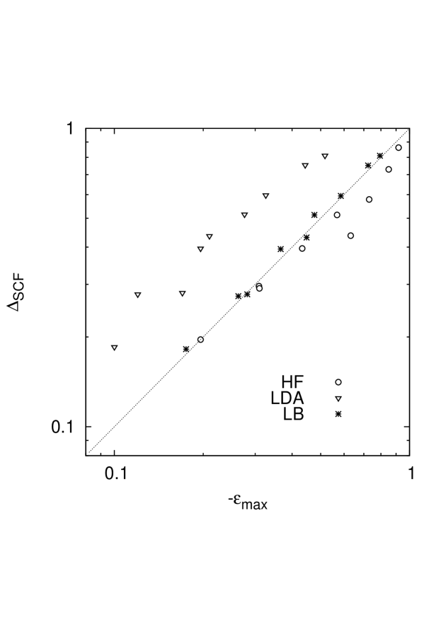
Figure 1: Plot of $\epsilon_{max}$ vs. $\Delta$SCF energies using different exchange-only potentials.

Next, motivated by the work of Ref. stein-eisenberg-kronik-baer:2010 , we tune the parameter $\beta$ in the LB potential so that $\epsilon_{max}$ matches with the $\Delta$SCF energies. The optimized $\beta$ and the corresponding energies are also shown in Table 1. As is evident from Table 1, choosing $\beta$ through IP theorem, the highest orbital energy $\epsilon_{max}$ improves. We note that according to Koopmans theorem Koopmans:1934 , the orbital energy $\epsilon_{i}$ is close to the removal energy of the electron from that orbital. However we find that DFT results are better in this regard. The results of Table 1 are depicted in Fig. 1 where we have plotted the $\Delta$SCF results against $-\epsilon_{max}$ for LSD, LB and HF theories. We see that the LB results are closest to the $\Delta$SCF$=-\epsilon_{max}$ line.

Having presented our results for the exchange-only calculations we next include correlation using the LDA. The correlation functional we use is that parametrized by Vosko, Wilk and Nusair vosko-wilk-nusair:1980 . The orbital energies $\epsilon_{max}$ and the $\Delta$SCF energies for the LB and $\beta$ optimized LB are presented in Table 2 in comparison with the experimental results w2012crc .

We see from Table 2 that with the asymptotically corrected LB potential, the IP theorem is satisfied remarkably well. The parameter $\beta$ in the LB potential is tuned to satisfy IP theorem (Ref. Eq. (1)) The $\epsilon_{max}$, so obtained matches with experiments in a much better way.

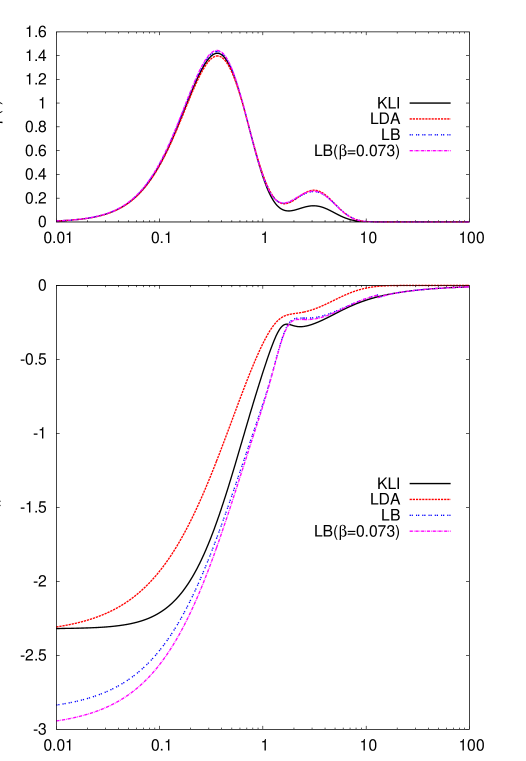
Figure 2: Ground-state radial density and the exchange potential of Li ($2s^{1}\ 2S$) for the up spin obtained using different approximations for the potential.

The radial density and the exchange potential for Li ground-state obtained using the LDA and the LB potentials are shown in Fig. 2. Also shown in Fig. 2 is the KLI potential krieger-li-iafrate:1992a , which is essentially the exact exchange potential, for comparison. It is evident that from about $r=0.2a.u.$ onwards, the LB potentials with both $\beta=0.05$ and the optimized $\beta$ are quite close to the KLI potential. The discrepancy of the LB potential for $r<0.2a.u$ corresponds to the non-zero $\beta$. Furthermore, all the three potentials go as $-1/r$ in the asymptotic regions. On the other hand, the LSD potential underestimates the exact potential all over. The bump in the potential for Li is at the minimum in the radial densities lindgren:1971 .

Having given the results for the ground-states, we now turn our attention to excited-states and show that the exchange functional and potential constructed for these states by splitting the $k$-space for HEG give results with similar accuracy.

III Split $k$-space method for constructing excited-state energy functionals and excited-state potential

In eDFT, we have put forth the idea that the excited state energies be calculated using the modified local spin density (MLSD) functional developed over the past few years samal-harbola:2005 ; shamim-harbola:2010 ; hemanadhan-harbola:2010 ; hemanadhan-harbola:2012 . The basis of the MLSD exchange energy functional is the split $k$-space method inbook:Harbola-etal:Ghosh-Chattaraj:2013 . In this method, the $k$-space is split in accordance to the orbital occupation of a given excited-state. In Fig. 3, we show an excited-state, where some orbitals (core) are occupied, followed by vacant (unocc) orbitals and then again orbitals are occupied (shell). To construct excited-state functionals, the density for each point is mapped onto the $k$-space of an HEG. The corresponding split $k$-space, also shown in Fig. 3, is constructed according to the orbital occupation i.e. the $k$-space is occupied from $0$ to $k_{1}$, vacant from $k_{1}$ to $k_{2}$ and then again occupied from $k_{2}$ to $k_{3}$ where $k_{1},k_{2},k_{3}$ are given by

$$k_{1}^{3}(\mathbf{r}) =3\pi^{2}\rho_{c}(\mathbf{r})$$ (8)

$$k_{2}^{3}(\mathbf{r})-k_{1}^{3}(\mathbf{r}) =3\pi^{2}\rho_{v}(\mathbf{r})$$ (9)

$$k_{3}^{3}(\mathbf{r})-k_{2}^{3}(\mathbf{r}) =3\pi^{2}\rho_{s}(\mathbf{r})$$ (10)

in terms of $\rho_{c}$, $\rho_{v}$ and $\rho_{s}$ corresponding to the electron densities of core, vacant (unoccupied) and the shell orbitals. Further,

$$\rho_{c}(\mathbf{r}) =\sum\limits^{n_{1}}_{i=1}{\left|\phi_{i}^{core}(\mathbf{r})\right|}^{2}$$ (11)

$$\rho_{v}(\mathbf{r}) =\sum\limits^{n_{2}}_{i=n_{1}+1}{\left|\phi_{i}^{unocc}(\mathbf{r})\right|}^{2}$$ (12)

$$\rho_{s}(\mathbf{r}) =\sum\limits^{n_{3}}_{i=n_{2}+1}{\left|\phi_{i}^{shell}(\mathbf{r})\right|}^{2}$$ (13)

where first $n_{1}$ orbitals are occupied, $n_{1}+1$ to $n_{2}$ are vacant followed by occupied orbitals from $n_{2}+1$ to $n_{3}$. The total electron density $\rho({\bf r})$ is given as

$$\rho({\mathbf{r}})=\rho_{c}({\mathbf{r}})+\rho_{s}({\mathbf{r}})$$ (14)

$$\textrm{or}\hskip 20.00003pt\rho({\mathbf{r}})=\rho_{1}({\mathbf{r}})-\rho_{2}({\mathbf{r}})+\rho_{3}({\mathbf{r}})$$ (15)

with $\rho_{1}=\rho_{c},\rho_{2}=\rho_{c}+\rho_{v}$ and $\rho_{3}=\rho_{c}+\rho_{v}+\rho_{s}$. Using this idea, we have constructed the kinetic hemanadhan-harbola:2010 and exchange-energy functionals samal-harbola:2005 for excited-states, and shown that these functionals lead to accurate kinetic, exchange, and transition energies. We point out that the application of the ground-state LSD functional generally leads to poor results for excited-states. The generality of this idea to construct energy functionals for other class of systems also leads to accurate energies shamim-harbola:2010 ; hemanadhan-harbola:2012 . Encouraged by these studies, we now subject this method to test by the IP theorem.

For this study, we consider the class of excited-systems as shown in Fig. 3 for which the MLSD functional is given by samal-harbola:2005

$$E_{X}^{MLDA}[\rho] =\int\rho(\mathbf{r})\left[\epsilon(k_{3})-\epsilon(k_{2})+\epsilon(k_{1})\right]d\mathbf{r}+\frac{1}{8\pi^{3}}\int\left(k_{3}^{2}-k_{1}^{2}\right)^{2}\ln\left(\frac{k_{3}+k_{1}}{k_{3}-k_{1}}\right)d\mathbf{r}$$

$$-\frac{1}{8\pi^{3}}\int\left(k_{3}^{2}-k_{2}^{2}\right)^{2}\ln\left(\frac{k_{3}+k_{2}}{k_{3}-k_{2}}\right)d\mathbf{r}+\frac{1}{8\pi^{3}}\int\left(k_{2}^{2}-k_{1}^{2}\right)^{2}\ln\left(\frac{k_{2}+k_{1}}{k_{2}-k_{1}}\right)d\mathbf{r}$$ (16)

where $\epsilon(k_{i})=\frac{-3k_{i}}{4\pi}$ is the exchange energy per particle for the ground state of HEG with Fermi wavevector $k_{i}$. Like the ground-state functional the modified local spin density (MLSD) functional is given as

$$E_{X}^{MLSD}[\rho]=\frac{1}{2}E_{X}^{MLDA}[2\rho_{\alpha}]+\frac{1}{2}E_{X}^{MLDA}[2\rho_{\beta}]$$ (17)

The corresponding potential $v^{MLSD}_{x}$ is given as

$$v_{x,\sigma}^{MLSD}(\textbf{r})=\frac{\delta E_{X}^{MLSD}[\rho]}{\delta\rho_{\sigma}(\mathbf{r})}$$ (18)

However, it has not been possible to get a workable analytical expression for $v_{x}^{MLSD}({\bf r})$ out of Eqs. (16) and (18). Therefore on the basis of arguments based on ground-state theory, we try to model the potential. For completeness we note the earlier attempts to construct accurate excited-state potentials by Gaspar gaspar:1974 and Nagy nagy:1990 . They have given an ensemble averaged exchange potential for the excited states and using this potential, they calculate excitation energy for single electron excitations. In the next section we propose an excited-state LDA-like exchange potential based on split $k$-space. This potential is similar to its ground-state LDA counterpart. We refer to this as the MLSD potential. We further correct the potential for its asymptotic behavior with the LB correction. With the asymptotically corrected MLSD potential, we show that the IP theorem for excited-states is satisfied to a good accuracy.

III.1 Generalization of Dirac exchange potential for excited-states using split $k$-space

The Hartree-Fock exchange potential for a system of electrons is given by

$$v_{x,i}^{HF}=v_{x}(\phi_{i})=-\sum_{j}\int\frac{\phi^{\ast}_{j}({\bf r^{\prime}})\phi_{i}({\bf r^{\prime}})\phi_{j}({\bf r})}{\phi_{i}({\bf r})|{\bf r}-{\bf r^{\prime}}|}d{\bf r^{\prime}}.$$ (19)

For homogeneous electron gas, the wavefunction is given by

$$\phi_{{\bf k}}({\bf r})=\frac{1}{{\sqrt{V}}}e^{\left(i{\bf k}\cdot{\bf r}\right)}.$$ (20)

where $V$ is the volume of the system. Using this form of wavefunction in Eq. (19) we get an exchange potential for one-gap systems shown in Fig. 3 to be for $\phi_{k}(\mathbf{r})$

$$v_{x}(k)= -\frac{1}{\pi}\left[k_{1}-k_{2}+k_{3}+\frac{k_{1}^{2}-k^{2}}{2k}\ln\left|\frac{k+k_{1}}{k-k_{1}}\right|\right.-\left.\frac{k_{2}^{2}-k^{2}}{2k}\ln\left|\frac{k+k_{2}}{k-k_{2}}\right|+\frac{k_{3}^{2}-k^{2}}{2k}\ln\left|\frac{k+k_{3}}{k-k_{3}}\right|\right]$$ (21)

where $k_{1},k_{2}$, and $k_{3}$ are given by Eqns (8), (9), (10)

This potential is orbital dependent. To make this potential an orbital independent potential we draw the analogy from the ground state exchange potential, where the exact LDA potential is equal to the HF potential for highest occupied molecular orbital (HOMO).

$$v^{HF}_{x,i}(\mathbf{r})|_{i=max}=\frac{\delta E_{x}^{LDA}[\rho(\mathbf{r})]}{\delta\rho(\mathbf{r})}$$ (22)

Therefore we take the potential for the electron in HOMO as the exchange potential for all the electrons. For this we put $k=k_{3}$ in Eq. (21), and get the following expression for the MLSD exchange potential

$$v_{x}^{MLSD}= -\frac{k_{3}}{\pi}\left[1-x_{2}+x_{1}-\frac{1}{2}(1-x_{1}^{2})\ln\left|\frac{1+x_{1}}{1-x_{1}}\right|\right.\left.+\frac{1}{2}(1-x_{2}^{2})\ln\left|\frac{1+x_{2}}{1-x_{2}}\right|\right]$$ (23)

where, $x_{1}=\frac{k_{1}}{k_{3}},x_{2}=\frac{k_{2}}{k_{3}}$

The MLSD potential of Eq. (23) is also obtained by taking the functional derivative of the exchange functional $E_{x}^{MLDA}$ of Eq. (16) with respect to $\rho_{3}(\mathbf{r})$, corresponding to the largest wave-vector in the $k$-space. Thus, we reach the same result from two different paths; this in some sense assures us about the correctness of the approach taken. When this potential is corrected for its asymptotic behavior by adding the LB correction, we obtain the modified LB (MLB) potential.

In the following Section, we test the MLB potential using the IP theorem for excited-states and show that it satisfies the IP theorem as accurately as the LB potential does for the ground-states. On the other hand, the LB potential does not lead to as accurate as satisfaction of the IP theorem indicating thereby that the potential derived on the basis of splitting $k$-space is more appropriate for the excited-state calculations.

IV Results for excited-states

The MLSD potential is the ground-state counterpart of the LSD potential. To correct the potential in the asymptotic region, we include the LB gradient term of Eq. (2) corresponding to largest wave-vector $k_{3}$ in the MLSD potential and obtain the MLB potential.

$$v_{x,\sigma}^{MLB}=v_{x}^{MLSD}-\beta\rho_{3,\sigma}^{1/3}(\mathbf{r})\frac{x^{2}_{3,\sigma}}{1+3\beta x_{3,\sigma}\sinh^{-1}(x_{3,\sigma})}$$ (24)

In performing self-consistent calculations, it is this potential that is employed as the exchange potential in the excited-state Kohn-Sham equations. Our calculations are performed using the central-field approximation Slater:1929 whereby the potential is taken to be spherically symmetric. Having obtained the orbitals the exchange energy is then calculated using the MLSDSIC functional samal-harbola:2005 and is given as

$$E_{X}^{MLSDSIC}=E_{X}^{MLSD}-\sum_{i}^{rem}{E_{i}}^{SIC}-\sum_{i}^{add}{E_{i}}^{SIC}$$ (25)

where,

$$E_{i}^{SIC}\left[\phi_{i}\right]=\int\int\frac{|\phi_{i}(\mathbf{r}_{1})|^{2}|\phi_{i}({\bf r}_{2})|^{2}}{|{\bf r}_{1}-{\bf r}_{2}|}d{\bf r}_{1}d{\bf r}_{2}+E^{LSD}_{X}\left[\rho\left(\phi_{i}\right)\right]$$ (26)

where the summation index $i$ in Eq. (25) runs over the orbitals from which the electrons are removed and create a gap, and to the orbitals to which the electrons are added. $E^{LSD}_{X}\left[\rho\left(\phi_{i}\right)\right]$ is the exchange energy corresponding to the $\phi_{i}$ orbital in the LSD approximation. Using the $\Delta$SCF energy obtained from these calculations and the eigenvalues from the Kohn-Sham calculations, we study the IP theorem. For our study, we have considered systems for which both the atomic excited-states and its ionic states can be represented by a single Slater determinant; this is so because LSD/MLSD is accurate for such states  barth:1979 .

Presented in Table 3 are the $\epsilon_{max}$ and $\Delta$SCF energies for different excited-states obtained using the LB potential of Eq. (6), and the excited-state MLB potential of Eq. (24). In both the LB and the MLB potentials, we have used $\beta=0.05$. Further, the energies for both the potentials are calculated using the MLSDSIC exchange energy functional. The HF $\epsilon_{max}$ and $\Delta$SCF are also shown in Table 3 for comparison. The results of Table III are shown graphically in Fig. 4. It is evident from the figure that the MLB potential satisfies the IP theorem accurately while the LB and HF both deviate from it. Thus accounting for the occupation of orbitals in the $k$-space gives better results for the theorem. Let us next check how does the MLB potential compare with the KLI potential for excited-states.

Plotted in Fig. 5 are the radial density and the corresponding excited-state exchange potential of Li $(3s^{1}\ {}^{2}S)$ within the LB and the MLB approximations. Also shown in the figure the exact exchange potential, obtained through KLI method Nagy:1997 . It is clear from the figure that the split $k$-space based MLB potential has a structure resembling the KLI potential for the excited-state: very close to it in the inter-shell region from about 0.1 a.u. onwards and beyond. This is similar to the relation between the LB potential and the KLI potential for the ground-states. The LB potential for the excited-states, on the other hand, is not close to the exact potential and has undesirable features at the minimum of radial density which are not present in the MLB potential. Similar unsmooth behavior is observed cheng-Wu-Voorhis:2008 in the LSD potential. In addition, the MLB potential is closer to the KLI potential in the interstitial and the asymptotic region, similar to what the LB potential did for the ground-states. The discrepancy between the potentials near the nucleus that was present in the ground-states is also present here. Nonetheless it is clear that the exchange potentials obtained on the basis of split $k$-space give a much better description of an excited-state than the ground-state LB potential.

To sum up, we have shown that excited-state energy functional and its asymptotically corrected potential based on split $k$-space satisfy IP theorem with a great accuracy in the exchange-only limit. This can be improved further by optimizing $\beta$. In Table 3, we also present the results obtained by varying the parameter $\beta$ in the excited-state MLB potential until $\epsilon_{max}$ matches with the $\Delta$SCF energies. The $\epsilon_{max}$ so obtained using the excited-state potential is close to the HF values. For $B\ (3p^{1}\ {}^{2}P)$ we are unable to tune the $\beta$ using the MLB potential.

We now wish to include correlation and compare our results with experiments. The lack of correlation potential for excited-states forces us to rely on the ground-state potential. In Table 4 are the calculations performed using the ground-state VWN potential. It is seen that similar to the ground-state, the $\Delta$SCF energies obtained with the split $k$-space functional are close to the experimental values. Also shown in table are the $\beta$ tuned energies to satisfy IP theorem. By imposing IP theorem, $\epsilon_{max}$ improves over the $\beta=0.05$ values and is closer to the experimental values for all atoms.

V Concluding Remarks

To conclude we have shown that splitting $k$-space according to the occupation of Kohn-Sham orbitals is a good way of constructing excited-state potential. The potential so constructed, when corrected for its long-range behavior, gives highly accurate eigenvalues for the upper most orbital in the sense of IP theorem: the eigenvalues and the $\Delta$SCF energies obtained from the energy functional by splitting $k$-space agree with one another to a great degree. This shows that split $k$-space method could be the proper path to follow for constructing excited-state energy functionals.

VI Acknowledgments

M. Hemanadhan wishes to thank Council of Scientific and Industrial Research (CSIR), New Delhi for financial support.

Figure 3: (a) Orbital and (b) the corresponding $k$-space occupation in the excited state configuration of a homogeneous electron gas (HEG).

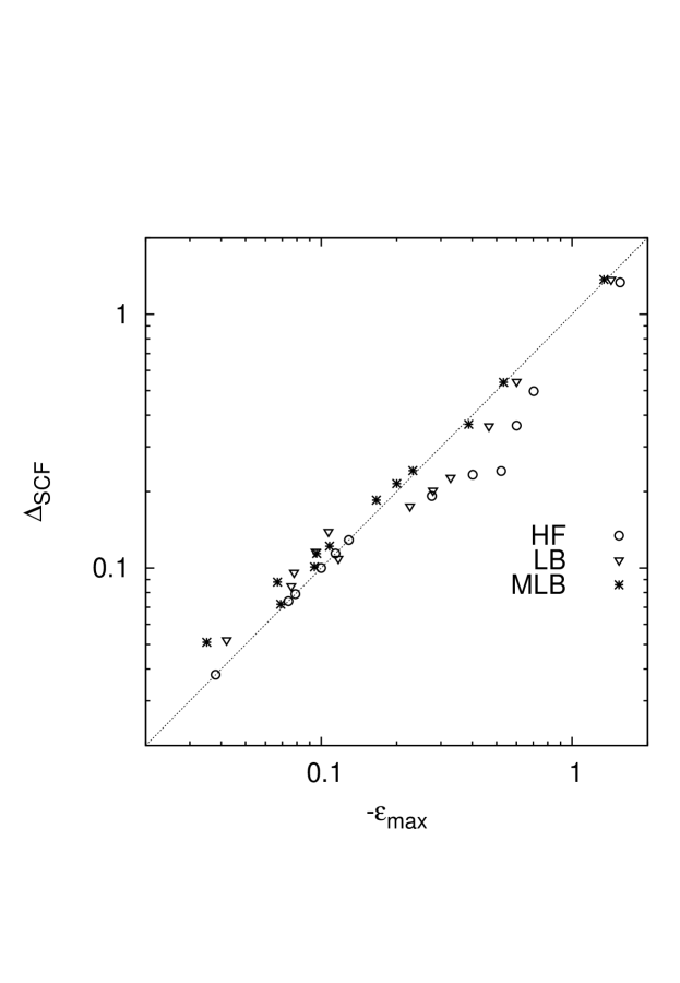
Figure 4: Plot of $\epsilon_{max}$ vs. $\Delta$SCF energies using different exchange-only potentials of LB, MLB and HF.

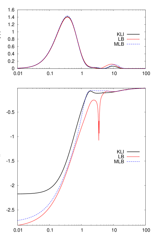
Figure 5: Excited-state radial density and the exchange potential of Li ($3s^{1}\ 2S$) for the up spin obtained using different approximations for the potential.

Table 1: Comparison of highest occupied eigen value $\epsilon_{\textrm{max}}$ and the $\Delta$SCF energies for atoms in their ground-state calculated using different exchange-only potentials. These are compared with the corresponding HF values. The numbers in $4^{th}$ and $5^{th}$ column are obtained with $\beta=0.05$ in Eq. (6) while those in column $7$ are obtained by optimizing $\beta$. The corresponding $\beta$ values are given in column $6$. (All the energies are in a.u)

Atoms/ion	LDA		LB($\beta=0.05$)		LB($\beta$)		HF
	$-\epsilon_{\textrm{max}}$	$\Delta$SCF	$-\epsilon_{\textrm{max}}$	$\Delta$SCF	$\beta$	$-\epsilon_{\textrm{max}}(=\Delta\textrm{SCF})$	$-\epsilon_{\textrm{max}}$	$\Delta$SCF
He($1s^{2}\ {}^{1}S$)	0.517	0.811	0.794	0.810	0.064	0.809	0.918	0.862
Li($2s^{1}\ {}^{2}S$)	0.100	0.185	0.175	0.182	0.073	0.182	0.196	0.196
Be($2s^{2}\ {}^{1}S$)	0.170	0.281	0.282	0.278	0.043	0.278	0.309	0.296
B($2s^{2}2p^{1}\ {}^{2}P$)	0.120	0.278	0.263	0.274	0.075	0.273	0.310	0.291
C($2s^{2}2p^{2}\ {}^{3}P$)	0.196	0.396	0.366	0.394	0.104	0.392	0.433	0.396
N($2s^{2}2p^{3}\ {}^{4}S$)	0.276	0.515	0.476	0.513	0.112	0.511	0.568	0.513
O($2s^{2}2p^{4}\ {}^{3}P$)	0.210	0.436	0.448	0.431	0.035	0.432	0.632	0.437
F($2s^{2}2p^{5}\ {}^{2}P$)	0.326	0.597	0.585	0.594	0.060	0.594	0.730	0.578
Ne($2s^{2}2p^{6}\ {}^{1}S$)	0.443	0.754	0.724	0.751	0.077	0.749	0.850	0.729

Table 2: Highest occupied eigen value $\epsilon_{\textrm{max}}$ and the $\Delta$SCF energies for atoms in their ground-states calculated using van Leeuwen and Baerends exchange and VWN correlation potential with the parameter $\beta=0.05$, and $\beta$ tuned, with the experimental values. (All the energies are in a.u)

Atom	LB-VWN($\beta=0.05$)		LB-VWN($\beta$)		Expt. w2012crc
	$-\epsilon_{\textrm{max}}$	$\Delta$SCF	$\beta$	$-\epsilon_{\textrm{max}}(=\Delta\textrm{SCF})$
He($1s^{2}\ {}^{1}S$)	0.851	0.892	0.106	0.890	0.904
Li($2s^{1}\ {}^{2}S$)	0.193	0.198	0.066	0.198	0.198
Be($2s^{2}\ {}^{1}S$)	0.320	0.329	0.072	0.329	0.342
B($2s^{2}2p^{1}\ {}^{2}P$)	0.296	0.312	0.086	0.311	0.305
C($2s^{2}2p^{2}\ {}^{3}P$)	0.401	0.431	0.115	0.430	0.414
N($2s^{2}2p^{3}\ {}^{4}S$)	0.511	0.550	0.117	0.548	0.534
O($2s^{2}2p^{4}\ {}^{3}P$)	0.516	0.506	0.041	0.507	0.501
F($2s^{2}2p^{5}\ {}^{2}P$)	0.647	0.661	0.065	0.660	0.640
Ne($2s^{2}2p^{6}\ {}^{1}S$)	0.782	0.813	0.082	0.811	0.792

Table 3: Highest occupied eigen value $\epsilon_{\textrm{max}}$ and the $\Delta$SCF energies for atoms in different excited-states calculated using different exchange-only potentials. These are compared with the corresponding HF values. The numbers in $2^{nd}$ and $3^{rd}$ column are obtained with $\beta=0.05$ in Eq. (6), in $4^{th}$ and $5^{th}$ column are obtained with $\beta=0.05$ in Eq. (24), while in column $5$ are obtained by optimizing $\beta$. The corresponding $\beta$ values are given in column $4$. (All the energies are in a.u)

Atom	LB($\beta=0.05$)		MLB($\beta=0.05$)		MLB($\beta$)		HF
	$-\epsilon_{\textrm{max}}$	$\Delta$SCF	$-\epsilon_{\textrm{max}}$	$\Delta$SCF	$\beta$	$-\epsilon_{\textrm{max}}(={\Delta\textrm{SCF})}$	$-\epsilon_{\textrm{max}}$	$\Delta$SCF
Li($2p^{1}\ {}^{2}P$)	0.117	0.109	0.096	0.114	0.300	0.114	0.129	0.129
B($2s^{1}2p^{2}\ {}^{2}D$)	0.226	0.175	0.166	0.185	0.120	0.183	0.276	0.192
C($2s^{1}2p^{3}\ {}^{3}D$)	0.279	0.202	0.200	0.215	0.090	0.213	0.402	0.233
N($2s^{1}2p^{4}\ {}^{4}P$)	0.328	0.227	0.232	0.242	0.070	0.241	0.522	0.241
O($2s^{1}2p^{5}\ {}^{3}P$)	0.466	0.362	0.387	0.368	0.035	0.370	0.601	0.364
F($2s^{1}2p^{6}\ {}^{2}S$)	0.601	0.543	0.533	0.539	0.055	0.538	0.703	0.497
Ne+($2s^{1}2p^{6}\ {}^{2}S$)	1.429	1.369	1.339	1.370	0.075	1.369	1.553	1.334
Li($3s^{1}\ {}^{2}S$)	0.076	0.085	0.069	0.072	0.080	0.073	0.074	0.074
Li($4s^{1}\ {}^{2}S$)	0.042	0.052	0.035	0.051	0.122	0.038	0.038	0.038
B($3s^{1}\ {}^{2}S$)	0.107	0.139	0.108	0.122	0.200	0.121	0.114	0.114
B($3p^{1}\ {}^{2}P$)	0.078	0.096	0.067	0.088	-	-	0.079	0.079
Be($2s^{1}3s^{1}\ {}^{3}S$)	0.095	0.116	0.094	0.101	0.100	0.102	0.100	0.100

Table 4: Comparison of highest occupied eigen value $\epsilon_{\textrm{max}}$ and the $\Delta$SCF energies for atoms in various excited-states calculated using MLB exchange-only potential with VWN correlation potential with the experimental values. The numbers in $2^{nd}$ and $3^{rd}$ column are obtained with $\beta=0.05$ in Eq. (24) while those in column $5$ are obtained by optimizing $\beta$. The corresponding $\beta$ values are given in column $4$. (All the energies are in a.u)

Atom	MLB-VWN($\beta=0.05$)		MLB-VWN($\beta$)
	$-\epsilon_{\textrm{max}}$	$\Delta$SCF	$\beta$	$-\epsilon_{\textrm{max}}(=\Delta\textrm{SCF})$	Expt. NIST
Li($2p^{1}\ {}^{2}P$)	0.110	0.128	0.230	0.127	0.130
B($2s^{1}2p^{2}\ {}^{2}D$)	0.214	0.252	0.600	0.247	0.257
C($2s^{1}2p^{3}\ {}^{3}D$)	0.262	0.300	0.500	0.295	0.318
N($2s^{1}2p^{4}\ {}^{4}P$)	0.308	0.344	0.350	0.339	0.348
O($2s^{1}2p^{5}\ {}^{3}P$)	0.453	0.441	0.040	0.442	0.471
F($2s^{1}2p^{6}\ {}^{2}S$)	0.594	0.604	0.056	0.600	0.623
Ne+($2s^{1}2p^{6}\ {}^{2}S$)	1.409	1.444	0.080	1.443	1.442
Li($3s^{1}\ {}^{2}S$)	0.079	0.081	0.060	0.081	0.074
Li($4s^{1}\ {}^{2}S$)	0.042	0.046	0.122	0.046	0.039
B($3s^{1}\ {}^{2}S$)	0.123	0.136	0.200	0.136	0.122
B($3p^{1}\ {}^{2}P$)	0.079	0.099	-	-	0.083
Be($2s^{1}3s^{1}\ {}^{3}S$)	0.107	0.112	0.082	0.112	0.105

References

- (1) R. G. Parr and W. Yang, Density-Functional Theory of Atoms and Molecules, Vol. 16 of International Series of Monographs on Chemistry (Oxford University Press, New York, 1989).
- (2) R. M. Dreizler and E. K. U. Gross, Density-Functional Theory: An Approach to the Quantum Many-Body Problem (Springer-Verlag, New York, 1990).
- (3) N. H. March, Electron Density Theory of Atoms and Molecules, Theoretical Chemistry Series (Academic Press, London, 1992).
- (4) E. Engel and R. M. Dreizler, Density Functional Theory: An Advanced Course, Theoretical and Mathematical Physics (Springer-Verlag, Berlin Heidelberg, 2011).
- (5) A. D. Becke, Phys. Rev. A 38, 3098 (1988).
- (6) J. P. Perdew, K. Burke, and M. Ernzerhof, Phys. Rev. Lett. 77, 3865 (1996), errata: Phys. Rev. Lett. 78, 1396 (1997).
- (7) J. Tau, J. P. Perdew, V. N. Staroverov, and E. Scuseria, Phys. Rev. Lett. 91, 146401 (2003).
- (8) R. van Leeuwen and E. J. Baerends, Phys. Rev. A 49, 2421 (1994).
- (9) N. Umezawa, Phys. Rev. A 74, 032505 (2006).
- (10) A. D. Becke and E. R. Johnson, J. Chem. Phys. 124, 221101 (2006).
- (11) C. A. Ullrich, Time-Dependent Density-Functional Theory: Concepts and Applications, Oxford Graduate Texts (Oxford University Press Inc., New York, 2012).
- (12) O. Gunnarsson and B. I. Lundqvist, Phys. Rev. B 13, 4274 (1976).
- (13) O. Gunnarsson and B. I. Lundqvist, Phys. Rev. B 15, 6006 (1977).
- (14) T. Ziegler, A. Rauk, and E. J. Baerends, Theor. Chim. Acta 43, 261 (1977).
- (15) U. von Barth, Phys. Rev. A 20, 1693 (1979).
- (16) A. K. Theophilou, J. Phys. C Solid State Phys. 12, 5419 (1979).
- (17) E. K. U. Gross, L. N. Oliveira, and W. Kohn, Phys. Rev. A 37, 2809 (1988).
- (18) L. N. Oliveira, E. K. U. Gross, and W. Kohn, Phys. Rev. A 37, 2821 (1988).
- (19) Á. Nagy, Phys. Rev. A 53, 3660 (1996).
- (20) A. Görling, Phys. Rev. A 59, 3359 (1999).
- (21) M. Levy and Á. Nagy, Phys. Rev. Lett. 83, 4361 (1999).
- (22) Á. Nagy and M. Levy, Phys. Rev. A 63, 052502 (2001).
- (23) M. Levy, Proc. Natl. Acad. Sci. USA 76, 6062 (1979).
- (24) M. K. Harbola, Phys. Rev. A 65, 052504 (2002).
- (25) M. K. Harbola, Phys. Rev. A 69, 042512 (2004).
- (26) P. Samal and M. K. Harbola, J. Phys. B: At. Mol. Opt. Phys. 38, 3765 (2005).
- (27) P. Samal and M. K. Harbola, Chem. Phys. Lett. 419, 217 (2006), errata: Chem. Phys. Lett. 422, 586 (2006).
- (28) P. Samal and M. K. Harbola, J. Phys. B: At. Mol. Opt. Phys. 39 4065 (2006).
- (29) M. Hemanadhan and M. K. Harbola, J. Mol. Struct. Theochem 943, 152 (2010).
- (30) M. Hemanadhan and M. Harbola, Eur. Phys. J. D 66, 1 (2012).
- (31) Md. Shamim and M. K. Harbola, J. Phys. B: At. Mol. Opt. Phys. 43, 215002 (2010).
- (32) J. P. Perdew, R. G. Parr, M. Levy, and J. L. Balduz, Phys. Rev. Lett. 49, 1691 (1982).
- (33) J. Katriel, E. R. Davidson, Proc. Natl. Acad. Sci. USA 77, 4403 (1980).
- (34) M. Levy, J. P. Perdew, and V. Sahni, Phys. Rev. A 30, 2745 (1984).
- (35) W. Haynes, D. R. Lide, and T. Bruno, CRC Handbook of Chemistry and Physics 2012-2013, CRC Handbook of Chemistry & Physics (CRC Press, Boca Raton, Florida, 2012).
- (36) A. Savin, in Recent advances in density functional methods: Part 1, Recent Advances in Computational Chemistry, Vol 1, Part 1, edited by D. Chong (World Scientific Publishing Company Incorporated, Singapore, 1995).
- (37) T. Leininger, H. Stoll, H.-J. Werner, and A. Savin, Chem. Phys. Lett. 275, 151 (1997).
- (38) H. Iikura, T. Tsuneda, T. Yanai, and K. Hirao, J. Chem. Phys. 115, 3540 (2001).
- (39) T. Yanai, D. P. Tew, and N. C. Handy, Chem. Phys. Lett. 393, 51 (2004).
- (40) R. Baer and D. Neuhauser, Phys. Rev. Lett. 94, 043002 (2005).
- (41) L. Kronik, T. Stein, S. Refaely-Abramson, and R. Baer, J. Chem. Theory Comput. 8, 1515 (2012).
- (42) D. Bohm and D. Pines, Phys. Rev. 92, 609 (1953).
- (43) T. Stein, H. Eisenberg, L. Kronik, and R. Baer, Phys. Rev. Lett. 105, 266802 (2010).
- (44) P. Singh, M. K. Harbola, B. Sanyal, and A. Mookerjee, Phys. Rev. B 87, 235110 (2013).
- (45) M. K. Harbola, M. Hemanadhan, Md. Shamim, and P. Samal, in Concepts and Methods in Modern Theoretical Chemistry, Electronic Structure and Reactivity, edited by S. K. Ghosh and P. K. Chattaraj (Taylor & Francis Group, Boca Raton, Florida, 2013).
- (46) C.-L. Cheng, Q. Wu, and T. V. Voorhis, J. Chem. Phys. 129, 124112 (2008).
- (47) A. Banerjee and M. K. Harbola, Phys. Rev. A 60, 3599 (1999).
- (48) P. A. M. Dirac, Proc. Cambridge Phil. Soc. 26, 376 (1930).
- (49) M. Levy and J. P. Perdew, Phys. Rev. A 32, 2010 (1985).
- (50) A. P. Gaiduk, S. K. Chulkov, and V. N. Staroverov, J. Chem. Theory Comput. 5, 699 (2009).
- (51) T. C. Koopmans, Physica 1, 104 (1934).
- (52) S. H. Vosko, L. Wilk, and M. Nusair, Can. J. Phys. 58, 1200 (1980).
- (53) J. B. Krieger, Y. Li, and G. J. Iafrate, Phys. Rev. A 45, 101 (1992).
- (54) I. Lindgren, Int. J. Quan. Chem. 5, 411 (1971).
- (55) R. Gáspár, Acta Phys. Hung. 35, 213 (1974).
- (56) Á. Nagy, Phys. Rev. A 42, 4388 (1990).
- (57) J. C. Slater, Phys. Rev. 34, 1293 (1929).
- (58) Á. Nagy, Phys. Rev. A 55, 3465 (1997).
- (59) A. Kramida, Y. Ralchenko, J. Reader, and N. A. Team, NIST Atomic Spectra Database (version 5.0), 2012.