Douglas–Rachford Feasibility Methods for
Matrix Completion Problems

Abstract

In this paper we give general recommendations for successful application of the Douglas–Rachford reflection method to convex and non-convex real matrix-completion problems. These guidelines are demonstrated by various illustrative examples.

Keywords

Douglas–Rachford, projections, reflections, matrix completion, feasibility problems, proteins reconstruction, Hadamard matrices

Mathematics Subject Classification (2010)

65K05, 90C59, 47N10

1 Introduction

Matrix completion may be posed as an inverse problem in which a matrix possessing certain properties is to be reconstructed knowing only a subset of its entries. A great many problems can be usefully cast within this framework (see [33, 36] and the references therein).

By encoding each of the properties which the matrix possesses along with its known entries as constraint sets, matrix completion can be cast as a feasibility problem. That is, it is reduced to the problem of finding a point contained in the intersection of a (finite) family of sets.

Projection algorithms comprise a class of general purpose iterative methods which are frequently used to solve feasibility problems (see [7] and the references therein). At each step, these methods utilize the nearest point projection onto each of the individual constraint sets. The philosophy here is that it is simpler to consider each constraint separately (through their nearest point projections), rather than the intersection directly.

Applied to closed convex sets in Euclidean space, the behaviour of projection algorithms is quite well understood. Moreover, their simplicity and ease of implementation has ensured continued popularity for successful applications in a variety of non-convex optimization and reconstruction problems [9, 10, 4]. This is despite the absence of sufficient theoretical justification, although there are some useful beginnings [16, 3, 28]. In many of these settings the Douglas–Rachford method (see Section 2.1) has been observed to perform better than other projection algorithms, and hence will be the projection algorithm of choice for this paper. A striking example of its better behaviour is detailed in Section 4.3.

We do note that there are many other useful projection algorithms, and many applicable variants. See for example, the method of cyclic projections [5, 8], Dykstra’s method [19, 6, 13], the cyclic Douglas–Rachford method [17], and many references contained in these papers.

In a recent paper [4], the present authors observed that many successful non-convex applications of the Douglas–Rachford method can be considered as matrix completion problems. The aim of this paper is to give general guidelines for successful application of the Douglas–Rachford method to a variety of (real) matrix reconstruction problems, both convex and non-convex.

The remainder of the paper is organised as follows: In Section 2 we first recall what is known about the Douglas–Rachford method, and then discuss our modelling philosophy. In Section 3 we consider several matrix completion problems in which all the constraint sets are convex: positive semi-definite matrices, doubly-stochastic matrices, Euclidean distance matrices; before discussing adjunction of noise. This is followed in Section 4 by a more detailed description of several classes in which some of the constraint sets are non-convex. In the first two subsections, we first look at low-rank constraints and then at low-rank Euclidean distance problems. In Section 4.3 we present a first detailed application by viewing protein reconstruction from NMR data as a low-rank Euclidean distance problem. The final three subsections of Section 4 carefully consider Hadamard, skew-Hadamard and circulant-Hadamard matrix problems, respectively. We end with various concluding remarks in Section 5.

2 Preliminaries

Let $E$ denote a finite dimensional Hilbert space – a Euclidean space. We will typically be considering the Hilbert space of real $m\times n$ matrices whose inner product is given by

$$\langle A,B\rangle:=\operatorname{tr}(A^{T}B),$$

where the superscript $T$ denotes the transpose, and $\operatorname{tr}(\cdot)$ the trace of an $n\times n$ square matrix. The induced norm is the Frobenius norm and can be expressed as

$$\|A\|_{F}:=\sqrt{\operatorname{tr}(A^{T}A)}=\sqrt{\sum_{i=1}^{n}\sum_{j=1}^{m}a_{ij}^{2}}.$$

A partial (real) matrix is an $m\times n$ array for which only entries in certain locations are known. A completion of the partial matrix $A=(a_{ij})\in\mathbb{R}^{m\times n}$, is a matrix $B=(b_{ij})\in\mathbb{R}^{m\times n}$ such that if $a_{ij}$ is specified then $b_{ij}=a_{ij}$. The problem of (real) matrix completion is the following: Given a partial matrix find a completion having certain properties of interest (e.g. positive semi-definite).

Throughout this paper, we formulate matrix completion as a feasibility problem. That is,

$$\text{Find }X\in\bigcap_{i=1}^{N}C_{i}\subseteq\mathbb{R}^{m\times n}.$$ (1)

Let $A$ be the partial matrix to be completed. We will take $C_{1}$ to be the set of all completions of $A$, and the sets $C_{2},\dots,C_{N}$ will be chosen such that their intersection has the properties of interest. In this case, (1) is precisely the problem of matrix completion.

2.1 The Douglas–Rachford method

Recall that the nearest point projection onto $S\subseteq E$ is the (set-valued) mapping $P_{S}:E\to 2^{S}$ defined by

$$P_{S}x:=\mathop{\rm argmin}_{s\in S}\|s-x\|=\{s\in S:\|s-x\|=\inf_{y\in S}\|y-x\|\}.$$

The reflection with respect to $S$ is the (set-valued) mapping $R_{S}:E\to 2^{E}$ defined by

$$R_{S}:=2P_{S}-I,$$

where $I$ denotes the identity map.

In an abuse of notation, if $P_{S}x$ (resp. $R_{S}x$) is singleton we use $P_{S}x$ (resp. $R_{S}x$) to denote the unique nearest point.

We now recall what is know about the Douglas–Rachford method, as specialized to finite dimensional spaces.

Theorem 2.1 (Convex Douglas–Rachford iterations).

Suppose $A,B\subseteq E$ are closed and convex. For any $x_{0}\in E$ define

$$x_{n+1}:=T_{A,B}x_{n}\text{ where }T_{A,B}:=\frac{I+R_{B}R_{A}}{2}.$$

Then if:

1. $A\cap B\neq\emptyset$, $(x_{n})$ converges to a point $x$ such that $P_{A}x\in A\cap B$.

2. $A\cap B=\emptyset$, $\|x_{n}\|\to+\infty$.

Proof.

See, for example, [11, Th. 3.13]. ∎

The results of Theorem 2.1 can only be directly applied to the problem of finding a point in the intersection of two sets. For matrix completion problems formulated as feasibility problems with greater than two sets, we use a well known product space reformulation.

Example 2.1 (Product space reformulation).

For constraint sets $C_{1},C_{2},\dots,C_{N}$ define

$$D:=\{(x,x,\dots,x)\in E^{N}|x\in E\},\quad C:=\prod_{i=1}^{N}C_{i}.$$

We now have an equivalent feasibility problem since

$$x\in\bigcap_{i=1}^{N}C_{i}\iff(x,x,\dots,x)\in D\cap C.$$

Moreover, $T_{D,C}$ can be readily computed whenever $P_{C_{1}},P_{C_{2}},\dots,P_{C_{N}}$ can be since

$$P_{D}x=\left(\frac{1}{N}\sum_{i=1}^{N}x_{i}\right)^{N},\quad P_{C}x=\prod_{i=1}^{N}P_{C_{i}}x_{i}.$$

For further details see, for example, [4, Section 3]. $\Diamond$

In the non-convex setting there are some useful theoretical beginnings. For a Euclidean sphere and affine subspace, with the reflection performed first with respect the sphere, Borwein and Sims [16] show that, appropriately viewed, the Douglas–Rachford scheme converges locally. An explicit region of convergence was given by Aragón Artacho and Borwein [3] for $\mathbb{R}^{2}$. Hesse and Luke [28] obtained local convergence results using a relaxed local version of firm nonexpansivity and appropriate regularity conditions, assuming that the reflection is performed first with respect to a subspace. We note that varying the order of the reflection does not make a substantive difference.

2.2 Modelling philosophy

As illustrated for Sudoku and other NP-complete combinatorial problems in [4], there are typically many ways to formulate the constraint set for a given matrix completion problem. For example, by choosing different sets $C_{2},C_{3},\dots,C_{N}$, in (1), such that $\cap_{i=2}^{N}C_{i}$ has the properties of interest. To apply the Douglas–Rachford method, these sets will be chosen in such a way that their individual nearest point projections are succinctly simple to compute — ideally in closed form. There is frequently a trade-off between the number of sets in the intersection, and the simplicity of their projections. For example, one extreme would be to encode the property of interest in a single constraint set. In this case, it is likely that its projection is difficult to compute.

To illustrate this philosophy, consider the following example which we revisit in Section 3.2. Suppose the property of interest is the constraint

$$\left\{X\in\mathbb{R}^{m\times n}|X_{ij}\geq 0,\sum_{k=1}^{n}X_{kj}=1\text{ for }i=1,\dots,m\text{ and }j=1,\dots,n\right\}.$$

This set is equal to the intersection of $C_{2}$ and $C_{3}$ where

$$C_{2} :=\left\{X\in\mathbb{R}^{m\times n}|X_{ij}\geq 0\text{ for }i=1,\ldots,m\text{ and }j=1,\ldots,n\right\},$$

$$C_{3} :=\left\{X\in\mathbb{R}^{m\times n}|\sum_{i=1}^{n}X_{ij}=1\text{ for }j=1,\ldots,n\right\}.$$

Here the projections onto the cone $C_{2}$ and the affine space $C_{3}$ can be easily computed (see Section 3.2). In contrast, the projection directly onto $C_{2}\cap C_{3}$ amounts to finding the nearest point in the convex hull of the set of matrices having a one in each row and remaining entries zero. This projection is less straightforward, and has no explicit form. For details, see [20].

The order of the constraint sets in (1) also requires some consideration. For matrix completion problems with two constraints, we can and do directly apply the Douglas–Rachford method to $C_{1}\cap C_{2}$, with the reflection first performed with respect to the set $C_{1}$. For matrix completion problems with more than two constraints, we apply the Douglas–Rachford method to the product formulation of Example 2.1, with the reflection with respect to $D$ performed first. In this case, the solution is obtained by projecting onto $D$ and thus can be monitored by considering only a single product coordinate.

In non-convex applications, the problem formulation chosen often determines whether or not the Douglas–Rachford scheme can successfully solve the problem at hand always, frequently or never, see also [4]. Hence, in the rest of this paper we focus on naive or direct implementation of the Douglas-Rachford method while focusing on the choice of an appropriate model and the computation of the requisite projections/reflections. In a followup paper, we will look at more refined variants for our two capstone applications: to protein reconstruction and to Hadamard matrix problems.

3 Convex Problems

We now look, in order, at positive-definite matrices and correlation matrices, doubly-stochastic matrices, and Euclidean distance matrices before discussing adjunction of noise.

3.1 Positive semi-definite matrices

Let $S_{n}$ denote the set of real $n\times n$ symmetric matrices. Recall that a matrix $A=(A_{ij})\in\mathbb{R}^{n\times n}$ is said to be positive semi-definite if

$$A\in S_{n}\text{ and }x^{T}Ax\geq 0\text{ for all }x\in\mathbb{R}^{n}.$$ (2)

The set of all such matrices form a closed convex cone (see [14, Ex. 1, Sec. 1.2]), and shall be denoted by $S_{+}^{n}$. The Loewner partial order is defined on $S_{n}$ by taking $A\succeq B$ if $A-B\in S_{+}^{n}$. Recall that a symmetric matrix is positive semi-definite if and only if all its eigenvalues are non-negative.

Let us consider the matrix completion problem where only some entries of the positive semi-definite matrix $A$ are known, and denote by $\Omega$ the location of these entries (i.e. $(i,j)\in\Omega$ if $A_{ij}$ is known). Without loss of generality, we may assume that $\Omega$ is symmetric in the sense that $(i,j)\in\Omega$ if and only if $(j,i)\in\Omega$. Consider the convex sets

$$C_{1}:=\{X\in\mathbb{R}^{n\times n}|X_{ij}=A_{ij}\text{ for all }(i,j)\in\Omega\},\quad C_{2}:=S_{n}^{+}.$$ (3)

Then $X$ is a positive semi-definite matrix that completes $A$ if and only if $X\in C_{1}\cap C_{2}$.

The set $C_{1}$ is a closed affine subspace. Its projection is straightforward, and given pointwise by

$$P_{C_{1}}(X)_{ij}=\left\{\begin{array}[]{cc}A_{ij}&\text{if }(i,j)\in\Omega,\\ X_{ij}&\text{otherwise};\end{array}\right.$$ (4)

for all $i,j=1,\dots,n$.

Theorem 3.1 ([29, Th. 2.1]).

Let $X\in\mathbb{R}^{n\times n}$. Define $Y=(A+A^{T})/2$ and let $Y=UP$ be a polar decomposition (see [29, Th. 1.1]). Then

$$P_{C_{2}}(X)=\frac{Y+P}{2}.$$ (5)

Remark 3.1.

For $X\in S_{n}$, $Y=X$ in the statement of Theorem 3.1. If this is the case, the computation of $P_{C_{2}}$ is also simplified.

If the initial matrix is symmetric, then the corresponding Douglas–Rachford iterates are too. This condition can be easily satisfied. For instance, if $X\in\mathbb{R}^{n\times n}$ then the iterates can instead be computed starting at $P_{S_{n}}(X)=(X+X^{T})/2$ or $XX^{T}\in S_{n}$.

Of course, for symmetric iterates only the the upper (or lower) triangular matrix need be computed. $\Diamond$

Remark 3.2.

The matrices $U$ and $P$ can also be easily obtained from a singular value decomposition (see [32, p. 205]). For if $Y=WSV^{T}$ is a singular value decomposition then

$$P=VSV^{T},\quad U=WV^{T}$$

produces $P$ and $U$. $\Diamond$

Remark 3.3 (Positive definite matrices).

Recall that a real symmetric $n\times n$ matrix is said to be positive definite if the inequality in (2) holds strictly whenever $x\neq 0$. Denote the set of all such matrices by $S^{n}_{++}$. Since $S^{n}_{++}$ is not closed, the problem of positive definite matrix completion cannot be directly cast within this framework by setting $C_{2}:=S^{n}_{++}$.

In practice, one might wish to consider a closed convex subset of $S_{++}^{n}$. For example, one could instead define

$$C_{2}:=\{X\in\mathbb{R}^{n\times n}|X^{T}=X,x^{T}Xx\geq\epsilon\|x\|^{2}\text{ for all }x\in\mathbb{R}^{n}\},$$ (6)

for some small $\epsilon>0$. Then (6) is equivalent to requiring that the eigenvalues be not less than $\epsilon$. $\Diamond$

One can apply our methods to finding semi-definite solutions to matrix Riccati equations [2].

3.1.1 Correlation matrices

An important class of positive semi-definite matrices is the correlation matrices. Given random variables $X_{1},X_{2},\dots,X_{n}$, the associated correlation matrix is an element of $[-1,1]^{n\times n}$ whose $ij$th entry is the correlation between variables $X_{i}$ and $X_{j}$. Since, any random variable perfectly correlates with itself, the entries along the main diagonal of any correlation matrix are all ones. Consequently,

$$\{(i,i)|i=1,\dots,n\}\subseteq\Omega,\text{ and }A_{ii}=1\text{ for }i=1,\dots,n.$$ (7)

Moreover whenever (7) holds, $A$ is necessarily contained in $[-1,1]^{n\times n}$. This is a consequence of the following inequality.

Proposition 3.1 ([32, p. 398]).

Let $A=(a_{ij})\in S^{n}_{+}$. Then

$$a_{ii}a_{jj}\geq a_{ij}^{2}.$$

Thus, if $A$ is an incomplete correlation matrix, without loss of generality we may assume that (7) holds. In this case, $X$ is correlation matrix that completes $A$ if and only if $X\in C_{1}\cap C_{2}$, as defined in (3).

Consider now the problem of generating a random sample of correlation matrices. This is the case, for example, when one uses simulation to determine an unknown probability distribution [1, 39].

The Douglas–Rachford method provides a heuristic for generating such a sample by applying the method to initial points chosen according to some probability distribution. In this case, the set of known indices, and their corresponding values, are

$$\Omega=\{(i,i)|i=1,\dots,n\},\text{ and }A_{ii}=1\text{ for }i=1,\dots,n.$$

The distribution of the entries in 100000 matrices of size $5\times 5$ obtained from three different sets of choices of initial point distribution is shown in Figure 1.

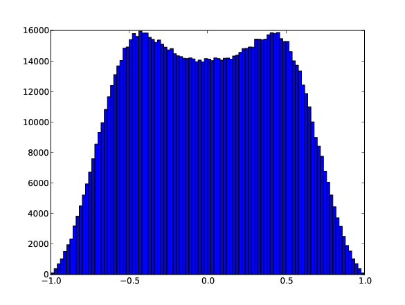
(a) $X_{0}:=Y$.

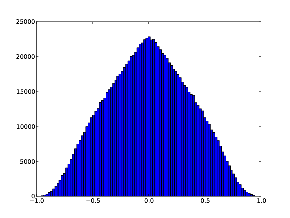
(b) $X_{0}:=(Y+Y^{T})/2$.

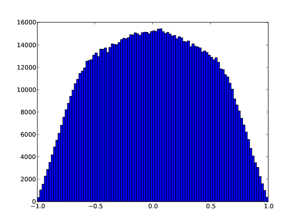
(c) $X_{0}:=YY^{T}$.

Figure 1: Distribution of entries in the collections of correlation matrices generated by different initialisations of the Douglas–Rachford algorithm. The initial point is $X_{0}$, and $Y$ is a random matrix in $[-1,1]^{5\times 5}$. Note $(Y+Y^{T})/2,YY^{T}\in S_{5}$.

3.2 Doubly stochastic matrices

Recall that a matrix $A=(A_{ij})\in\mathbb{R}^{m\times n}$ is said to be doubly stochastic if

$$\sum_{i=1}^{m}A_{ij}=\sum_{j=1}^{n}A_{ij}=1,A_{ij}\geq 0\text{ for }i=1,\dots,m\text{ and }j=1,\dots,n.$$ (8)

The set of all doubly stochastic matrices are known as the Birkhoff polytope, and can be realised as the convex hull of the set of permutation matrices (see, for example, [14, Th. 1.25]).

Let us now consider the matrix completion problem where only some entries of a doubly stochastic matrix $A$ are known, and denote by $\Omega$ the location of these entries (i.e., $(i,j)\in\Omega$ if $A_{ij}$ is known). The set of all such candidates is given by

$$C_{1} :=\{X\in\mathbb{R}^{m\times n}|X_{ij}=A_{ij}\text{ for all }(i,j)\in\Omega\},$$ (9)

which is similar to (3). The Birkhoff polytope may be expressed as the intersection of the three convex sets

$$C_{2} :=\left\{X\in\mathbb{R}^{m\times n}|\sum_{i=1}^{m}X_{ij}=1\text{ for }j=1,\dots,n\right\},$$ (10)

$$C_{3} :=\left\{X\in\mathbb{R}^{m\times n}|\sum_{j=1}^{n}X_{ij}=1\text{ for }i=1,\dots,m\right\},$$ (11)

$$C_{4} :=\{X\in\mathbb{R}^{m\times n}|X_{ij}\geq 0\text{ for }i=1,\dots,m\text{ and }j=1,\dots,n\}.$$ (12)

Then $X$ is a double stochastic matrix that completes $A$ if and only if $X\in C_{1}\cap C_{2}\cap C_{3}\cap C_{4}.$

As in (4), the set $C_{1}$ is a closed affine subspace whose projection is given pointwise by

$$P_{C_{1}}(X)_{ij}=\left\{\begin{array}[]{cc}A_{ij}&\text{if }(i,j)\in\Omega,\\ X_{ij}&\text{otherwise};\end{array}\right.$$ (13)

for all $i=1,\dots,m$ and $j=1,\dots,n$.

The projection onto $C_{2}$ (resp. $C_{3}$) can be easily computed by applying the following proposition row-wise (resp. column-wise).

Proposition 3.2.

Let $S:=\{x\in\mathbb{R}^{m}|\sum_{i=1}^{m}x_{i}=1\}$. For any $x\in\mathbb{R}^{m}$,

$$P_{S}(x)=x+\frac{1}{m}\left(1-\sum_{i=1}^{m}x_{i}\right)e,\text{ where }e=[1,1,\dots,1]^{T}.$$

Proof.

Since $S=\{x\in\mathbb{R}^{n}|\langle e,x\rangle=1\}$, the result follows from the standard formula for the orthogonal projection onto a hyperplane (see, for example, [22, Sec. 4.2.1]). ∎

The projection of $A$ onto $C_{4}$ is given pointwise by

$$P_{C_{4}}(A)_{ij}=\max\{0,A_{ij}\},$$

for $i=1,\dots,m$ and $j=1,\dots,n.$

Remark 3.4.

One can also address the problem of singly-stochastic matrix completion. The problem of row (resp. column) stochastic matrix completion is formulated by dropping constraint $C_{3}$ (resp. $C_{2}$). $\Diamond$

3.3 Euclidean distance matrices

A matrix $D=(D_{ij})\in\mathbb{R}^{n\times n}$ is said to be a distance matrix if

$$D_{ij}=D_{ji}=\left\{\begin{array}[]{cl}=0,&i=j,\\ \geq 0,&i\neq j;\end{array}\right.\text{ for }i,j=1,\dots,n.$$

Furthermore, $D$ is called a Euclidean distance matrix (EDM) if there are points $p_{1},\ldots,p_{n}\in\mathbb{R}^{r}$ (with $r\leq n$) such that

$$D_{ij}=\|p_{i}-p_{j}\|^{2}\quad\text{for }i,j=1,\ldots,n.$$ (14)

If (14) holds for a set of points in $\mathbb{R}^{r}$ then $D$ is said to be embeddable in $\mathbb{R}^{r}$. If $D$ is embeddable in $\mathbb{R}^{r}$ but not in $\mathbb{R}^{r-1}$, then it is said to be irreducibly embeddable in $\mathbb{R}^{r}$.

The following result by Hayden and Wells, based on Schoenberg’s criterion [40, Th. 1], provides a useful characterization of Euclidean distance matrices.

Theorem 3.2 ([27, Th. 3.3]).

Let $Q$ be the Householder matrix defined by

$$Q:=I-\frac{2vv^{T}}{v^{T}v},\text{ where }v=\left[1,1,\ldots,1,1+\sqrt{n}\right]^{T}\in\mathbb{R}^{n}.$$

Then, a distance matrix $D$ is a Euclidean distance matrix if and only if the ${(n-1)\times(n-1)}$ block $\widehat{D}$ in

$$Q(-D)Q=\left[\begin{array}[]{cc}\widehat{D}&d\\ d^{T}&\delta\end{array}\right]$$ (15)

is positive semidefinite. In this case, $D$ is irreducibly embeddable in $\mathbb{R}^{r}$ where $r=\operatorname{rank}(\widehat{D})\leq n-1$.

Remark 3.5.

As a consequence of Theorem 3.2, the set of Euclidean distance matrices is convex. $\Diamond$

Let us consider now the matrix completion problem where only some entries of a Euclidean distance matrix $D$ are known, and denote by $\Omega$ the location of these entries (i.e., $(i,j)\in\Omega$ if $D_{ij}$ is known). Without loss of generality we assume $D$ and $\Omega$ to be symmetric. Consider the convex sets

$$C_{1}:= \big{\{}X\in\mathbb{R}^{n\times n}\mid X\text{ is a distance matrix},X_{ij}=D_{ij}\text{ for all }(i,j)\in\Omega\big{\}},$$ (16)

$$C_{2}:= \big{\{}X\in\mathbb{R}^{n\times n}\mid\widehat{X}\succeq 0\text{ where }\widehat{X}\text{ is the block in }Q(-X)Q\text{ in }\eqref{eq:Q-DQ}\big{\}}$$ (17)

Then $X$ is a Euclidean distance matrix that completes $D$ if and only if $X\in C_{1}\cap C_{2}$.

The projection of any symmetric matrix $A=(A_{ij})\in\mathbb{R}^{n\times n}$ onto $C_{1}$ can be easily computed:

$$P_{C_{1}}(A)=\left\{\begin{array}[]{cl}0,&\text{if }i=j,\\ D_{ij},&\text{if }(i,j)\in\Omega,\\ \max\{0,A_{ij}\},&\text{otherwise;}\end{array}\right.$$ (18)

The projection of $A$ onto $C_{2}$ is the unique solution to the problem

$$\min_{X\in C_{2}}\|A-X\|_{F}.$$

If we denote

$$Q(-A)Q=\left[\begin{array}[]{cc}\widehat{A}&a\\ a^{T}&\alpha\end{array}\right]\quad\text{and}\quad Q(-X)Q=\left[\begin{array}[]{cc}\widehat{X}&x\\ x^{T}&\lambda\end{array}\right],$$

then

$$\min_{X\in C_{2}}\|A-X\|_{F} =\min_{X\in C_{2}}\|Q(A-X)Q\|_{F}=\min_{X\in C_{2}}\|Q(-A)Q-Q(-X)Q\|_{F}$$

$$=\min_{x\in\mathbb{R}^{n},\lambda\in\mathbb{R}\atop\widehat{X}=\widehat{X}^{T},\widehat{X}\succeq 0}\left\|\begin{array}[]{cc}\widehat{A}-\widehat{X}&a-x\\ (a-x)^{T}&(\alpha-\lambda)\end{array}\right\|_{F}.$$

A consequence of [27, Th. 2.1] is that the unique best approximation is given by

$$\left[\begin{array}[]{cc}U\Lambda_{+}U^{T}&a\\ a^{T}&\alpha\end{array}\right]$$

where $U\Lambda U^{T}=\widehat{A}$ is the spectral decomposition (see [27, p.116]) of $\widehat{A}$, with $\Lambda=\operatorname{diag}(\lambda_{1},\ldots,\lambda_{n-1})$, and $\Lambda_{+}=\operatorname{diag}(\max\{0,\lambda_{1}\},\ldots,\max\{0,\lambda_{n-1}\})$. Therefore,

$$P_{C_{2}}(A)=-Q\left[\begin{array}[]{cc}U\Lambda_{+}U^{T}&a\\ a^{T}&\alpha\end{array}\right]Q.$$ (19)

3.3.1 Noise

In many practical situations the distances that are initially known have some errors in their measurements, and the Euclidean matrix completion problem may not even have a solution. In these situations, a model that allows errors in the distances needs to be considered.

Given some error $\varepsilon\geq 0$, consider the convex set

$$C_{1}^{\varepsilon}:=\big{\{}X\in\mathbb{R}^{n\times n}\mid \,X\text{ is a distance matrix}$$

$$\text{ and }|X_{ij}-D_{ij}|\leq\varepsilon\text{ for all }(i,j)\in\Omega\big{\}}.$$ (20)

Notice that $C_{1}^{0}=C_{1}$. The projection of any symmetric matrix $A=(A_{ij})\in\mathbb{R}^{n\times n}$ onto $C_{1}^{\varepsilon}$ can be easily computed:

$$P_{C_{1}^{\varepsilon}}(A)=\left\{\begin{array}[]{cl}0,&\text{if }i=j,\\ D_{ij}+\varepsilon,&\text{if }(i,j)\in\Omega\text{ and }A_{ij}>D_{ij}+\varepsilon,\\ \max\{0,D_{ij}-\varepsilon\},&\text{if }(i,j)\in\Omega\text{ and }A_{ij}<D_{ij}-\varepsilon,\\ \max\{0,A_{ij}\},&\text{otherwise.}\end{array}\right.$$ (21)

This model could be easily modified to include a different upper and lower bound on each distance $D_{ij}$ for $(i,j)\in\Omega$.

4 Non-convex Problems

We now turn to the more difficult case of non-convex matrix completion problems.

4.1 Low-rank matrices

It many practical scenarios, one would like to recover a matrix that is known to be low-rank from only a subset of its entries. This is the case, for example, in various compressed sensing applications [15]. The main problem here is that the low-rank constraint makes the problem non-convex. For example, if we consider

$$S:=\big{\{}A\in\mathbb{R}^{2\times 2}\big{|}\operatorname{rank}(A)\leq 1\big{\}},$$

then

$$\left[\begin{array}[]{cc}1&0\\ 0&0\end{array}\right],\left[\begin{array}[]{cc}0&0\\ 0&1\end{array}\right]\in S,$$

but for all $\lambda\in(0,1)$,

$$\lambda\left[\begin{array}[]{cc}1&0\\ 0&0\end{array}\right]+(1-\lambda)\left[\begin{array}[]{cc}0&0\\ 0&1\end{array}\right]\not\in S.$$

4.1.1 Relaxed rank constraints

Let us consider the problem of finding a matrix of minimal rank, given that some of the entries are known. We define a relaxed rank constraint

$$C_{2}^{r}:=\{X\in\mathbb{R}^{m\times n}|\operatorname{rank}(X)\leq r\}.$$

Then $X$ is a matrix completion of $A$ with rank at most $r$ if and only if $X\in C_{1}\cap C_{2}^{r}$.

The set of possible ranks of $A$ is finite and bounded above by $\min\{m,n\}$. Furthermore, $C_{2}^{r}\subseteq C_{2}^{s}$ for $r\leq s$. It follows that $X$ is a completion of $A$ with minimal rank if and only if

$$X\in C_{1}\cap C_{2}^{r_{0}}\text{ and }X\not\in C_{1}\cap C_{2}^{r}\text{ for any }r<r_{0}.$$

In this case $\operatorname{rank}(X)=r_{0}$.

This suggests a binary search heuristic for finding the rank of a matrix. For convenience, abbreviate the Douglas–Rachford method by DR, and denote by $P^{(r)}$ the relaxation

$$\text{Find }x\in C_{1}\cap C_{2}^{r}.$$ (22)

The iteration can now be implemented as shown as Algorithm 1:

input : $\Omega$, $A_{ij}$ for all $(i,j)\in\Omega$, $MaxIterations$

$r_{lb}:=0,r_{ub}:=\min\{m,n\},r:=\lfloor r_{ub}/2\rfloor$;

while $r_{lb}<r_{ub}$ do

       if DR solves $P^{(r)}$ within $MaxIterations$ iterations  then

             $r_{ub}:=r$;

            

       else

             $r_{lb}:=r+1$;

            

       end if

      $r:=\lfloor(r_{lb}+r_{ub})/2\rfloor$;

      

end while

output : $r$

Algorithm 1 Heuristic for minimum rank matrix completion.

Of course there are many applicable variants on this idea. For instance, one could instead perform a ternary search.

4.2 Low-rank Euclidean distance matrices

In many situations, the Euclidean distance matrix $D$ that one aims to complete is known to be embeddable in $\mathbb{R}^{r}$, say with $r=3$. This is the case, for example, in the molecular conformation problem in which one would like to compute the relative atom positions within a molecule. Nuclear magnetic resonance spectroscopy can be employed to measure short range interatomic distances (i.e. those less than 5–6Å) without structural modification of the molecule (see [42]).

These types of problems are known as low-rank Euclidean distance matrix problems. For any given positive integer $r$, we can modify the set $C_{2}$ in (17) as follows

$$C_{2}^{r}:=\big{\{}X\in\mathbb{R}^{n\times n}\mid \,\widehat{X}\succeq 0\text{ where }\widehat{X}\text{ is the block}$$

$$\text{ in }Q(-X)Q\text{ in }\eqref{eq:Q-DQ}\text{ and }\operatorname{rank}(\widehat{X})\leq r\big{\}}.$$

Unfortunately, as noted in [24, §5.3], the set $C_{2}^{r}$ is no longer convex unless $r\geq n-1$ (in which case the rank condition is always satisfied and $C_{2}^{r}=C_{2}$). Nevertheless, a projection of any symmetric matrix $A$ onto $C_{2}^{r}$ can be easily computed. Indeed, let us assume without loss of generality that the eigenvalues $\lambda_{1},\ldots,\lambda_{n-1}$ of the submatrix $\widehat{X}$ are given in nondecreasing order $\lambda_{1}\leq\lambda_{2}\leq\ldots\leq\lambda_{n-1}$ in the spectral decomposition $\widehat{X}=U\Lambda U^{T}$, where $\Lambda=\operatorname{diag}(\lambda_{1},\ldots,\lambda_{n-1})$. Then, $P_{C_{2}^{r}}(X)$ can be computed as in (19) but with $\Lambda_{+}$ replaced by

$$\Lambda_{+}^{r}:=\operatorname{diag}(0,\ldots,0,\max\{0,\lambda_{n-r}\},\ldots,\max\{0,\lambda_{n-1}\}).$$

4.3 Protein reconstruction

Once more, despite the absence of convexity in one of the constraints, we have observed the Douglas–Rachford algorithm to converge. Computational experiments have been performed on various protein molecules obtained from the RCSB Protein Data Bank. The complete structure of these proteins is contained in the respective data files as a list of points in $\mathbb{R}^{3}$, each representing an individual atom. The corresponding complete Euclidean distance matrix can then be computed using (14). A realistic partial Euclidean distance matrix is then obtained by removing all entries which correspond to distances greater than 6Å. From this partial matrix, we seek to reconstruct the molecular conformation.

In Algorithm 2 we give details regarding our Python implementation for finding the distance matrix and in Algorithm 3 we reconstruct the positions from the matrix completion.

input : $D\in\mathbb{R}^{n\times n}$ (the partial Euclidean distance matrix)

$\epsilon:=0.1,\,r:=3,\,N:=5000,\,k:=0$;

$X:=(Y+Y^{T})/2\in S_{n}$ for random $Y\in[-1,1]^{n\times n}$;

while $k\leq N$ do

       $X:=T_{C_{1}^{\epsilon},C_{2}^{r}}X$;

       $k:=k+1$;

      

end while

output : $X$ (the reconstructed Euclidean distance matrix)

Algorithm 2 Douglas–Rachford component of our Python implementation.

The quality of the solution is then assessed using various error measurements. The relative error, reported in decibels (dB), is given by

$$\text{Relative error}:=10\log_{10}\left(\frac{\|P_{C_{2}^{r}}P_{C_{1}^{\epsilon}}X_{N}-P_{C_{1}^{\epsilon}}X_{N}\|_{F}^{2}}{\|P_{C_{1}^{\epsilon}}X_{N}\|_{F}^{2}}\right),\text{ where }\epsilon=0.1,r=3.$$

input : $X\in\mathbb{R}^{n\times n}$ (the reconstructed distances matrix)

$L:=I-ee^{T}/n$ where $e=(1,1,\dots,1)^{T}$;

$\tau:=-\frac{1}{2}LDL$;

$USV^{T}:=SingularValueDecomposition(\tau)$;

$Z:=$first $n$ columns of $U\sqrt{S}$;

$p_{i}:=i$th row of $Z$ for $i=1,2,\dots,n$;

output : $p_{1},p_{2},\dots,p_{n}$ (positions of the points in $\mathbb{R}^{n}$)

Algorithm 3 Converting a Euclidean distance matrix to points in $\mathbb{R}^{n}$ (see [18, Sec. 5.12]).

Let $p_{1},p_{2},\dots,p_{n}\in\mathbb{R}^{3}$ denote the positions of the $n$ atoms obtained from the distance matrix $X_{N}$, and let $p_{1}^{true},p_{2}^{true},\dots,p_{n}^{true}$ denote the true positions of the $n$ atoms (both relative to the same coordinate system). It is possible for both sets of points to represent the same molecular conformation without occupying the same positions in space. Thus, to compare the two sets, a Procrustes analysis is performed. That is, we (collectively) translate, rotate and reflect the points $p_{1},p_{2},\dots,p_{n}$ to obtain the point $\hat{p}_{1},\hat{p}_{2},\dots,\hat{p}_{n}$ which minimize the least squared error to the true positions.

Using the fitted points, we compute the root-mean-square error (RMSE) defined by

$$\text{RMSE}:=\sqrt{\frac{1}{\text{\# of atoms}}\sum_{i=1}^{m}\|\hat{p}_{i}-p_{i}^{true}\|_{2}^{2}},$$

and the maximum error defined by

$$\text{Max Error}:=\max_{1\leq i\leq m}\|\hat{p}_{i}-p_{i}^{true}\|_{2}.$$

Table 1: Six Proteins: average (maximum) errors from five replications (5000 iterations).

Protein	# Atoms	Relative Error (dB)	RMSE	Max Error
1PTQ	404	-83.6 (-83.7)	0.0200 (0.0219)	0.0802 (0.0923)
1HOE	581	-72.7 (-69.3)	0.191 (0.257)	2.88 (5.49)
1LFB	641	-47.6 (-45.3)	3.24 (3.53)	21.7 (24.0)
1PHT	988	-60.5 (-58.1)	1.03 (1.18)	12.7 (13.8)
1POA	1067	-49.3 (-48.1)	34.1 (34.3)	81.9 (87.6)
1AX8	1074	-46.7 (-43.5)	9.69 (10.36)	58.6 (62.6)

Our computational results are summarized in Table 1. An animation of the algorithm at work constructing the protein 1PTQ can be viewed at http://carma.newcastle.edu.au/DRmethods/1PTQ.html. We next make some general comments regarding the performance of our method.

• 1PTQ and 1HOE, the two proteins with less than 600 atoms, could be reliability reconstructed to within a small error. A visual comparison of the reconstructed and original molecules match well – they are indistinguishable. See Figures 2 and 3.

• The reconstructions of 1LFB and 1PHT, the next two smallest proteins examined, were both satisfactory although not as good as their smaller counterparts. A careful comparison of the original and reconstructed images in Figure 3, shows that a large proportion of the proteins have been faithfully reconstructed, although some finer details are missing. For instance, one should look at the top right corners of the 1PHT images.

• The reconstructions of 1POA and 1AX8, the largest two proteins examined, were poor. The images of the reconstructed proteins show that some bond lengths are abnormally large. We discuss possible approaches to this issue in Remarks 4.1 and 4.2.

• Some alternative approaches to protein reconstruction are reported in [23]. Three are:

  • A “build-up” algorithm placing atoms sequentially (Buildup).

  • A classical multidimensional scaling approach (CMDSCALE).

  • Global continuation on Gaussian smoothing of the error function (DGSOL).

  For 1PTQ and HOE, the RMS error of the Douglas–Rachford reconstruction was slightly smaller than the reconstruction obtained from either the buildup algorithm or CMDSCALE. For 1LFB and 1PHT the RMS errors were comparable, and for 1POA and 1AXE they still had the same order of magnitude. DGSOL performed better than all three approaches (Douglas–Rachford, Buildup and CMSCALE).

• For the proteins examined, computational times for the full 5000 iterations, except for 1POA, ran anywhere from 6 to 18 hours. This time is mostly consumed by eigen-decompositions performed as part of computing $P_{C_{2}^{r}}$ and could perhaps be dramatically reduced by using a cheaper approximate projection. For 1POA we used up to 50 hours for a full reconstruction.

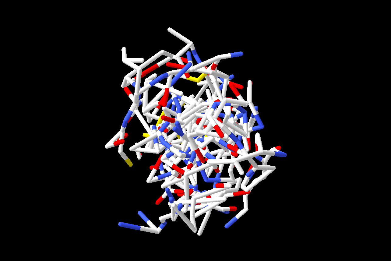
(a) 500 steps, -25 dB.

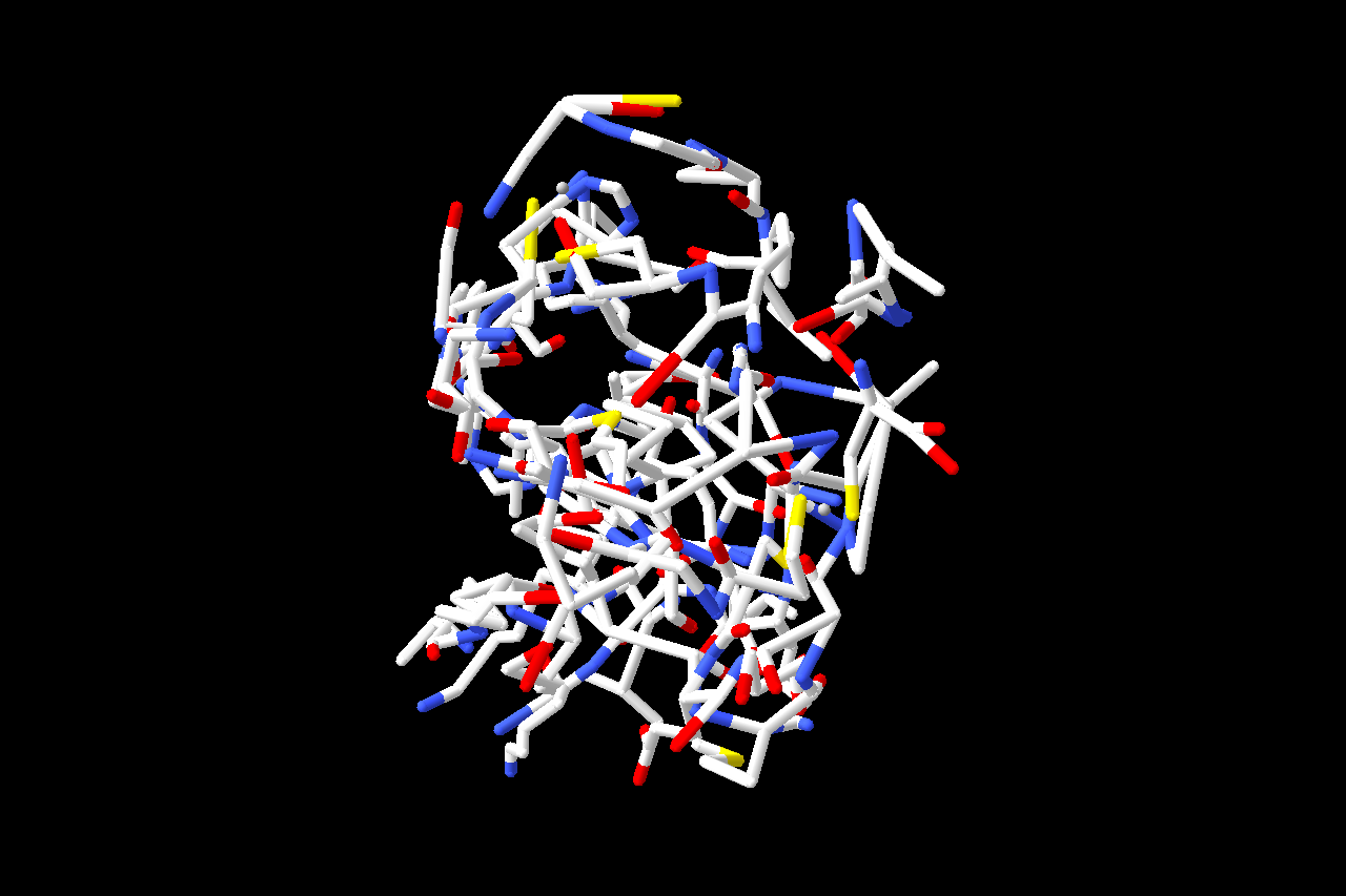
(b) 1,000 steps, -30 dB.

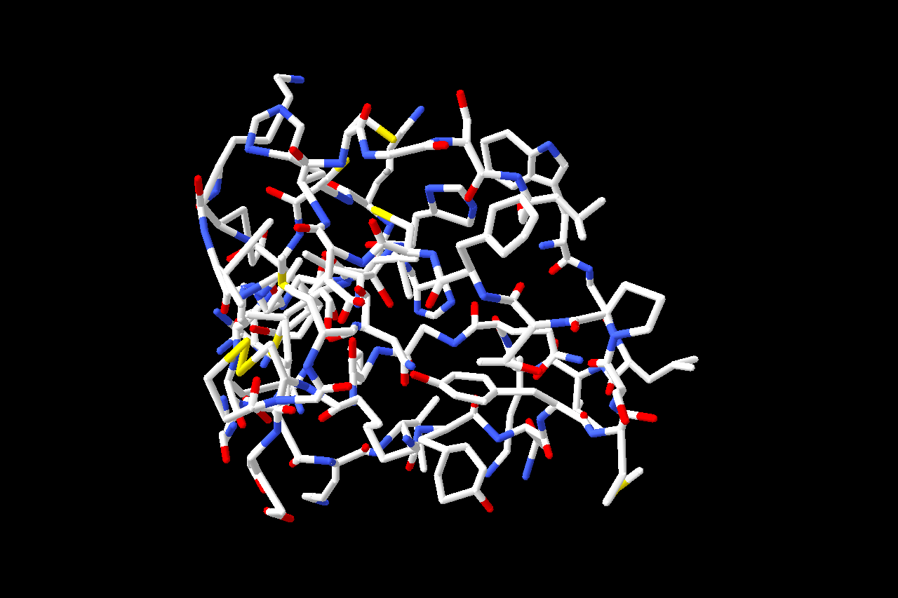
(c) 1,500 steps, -37 dB.

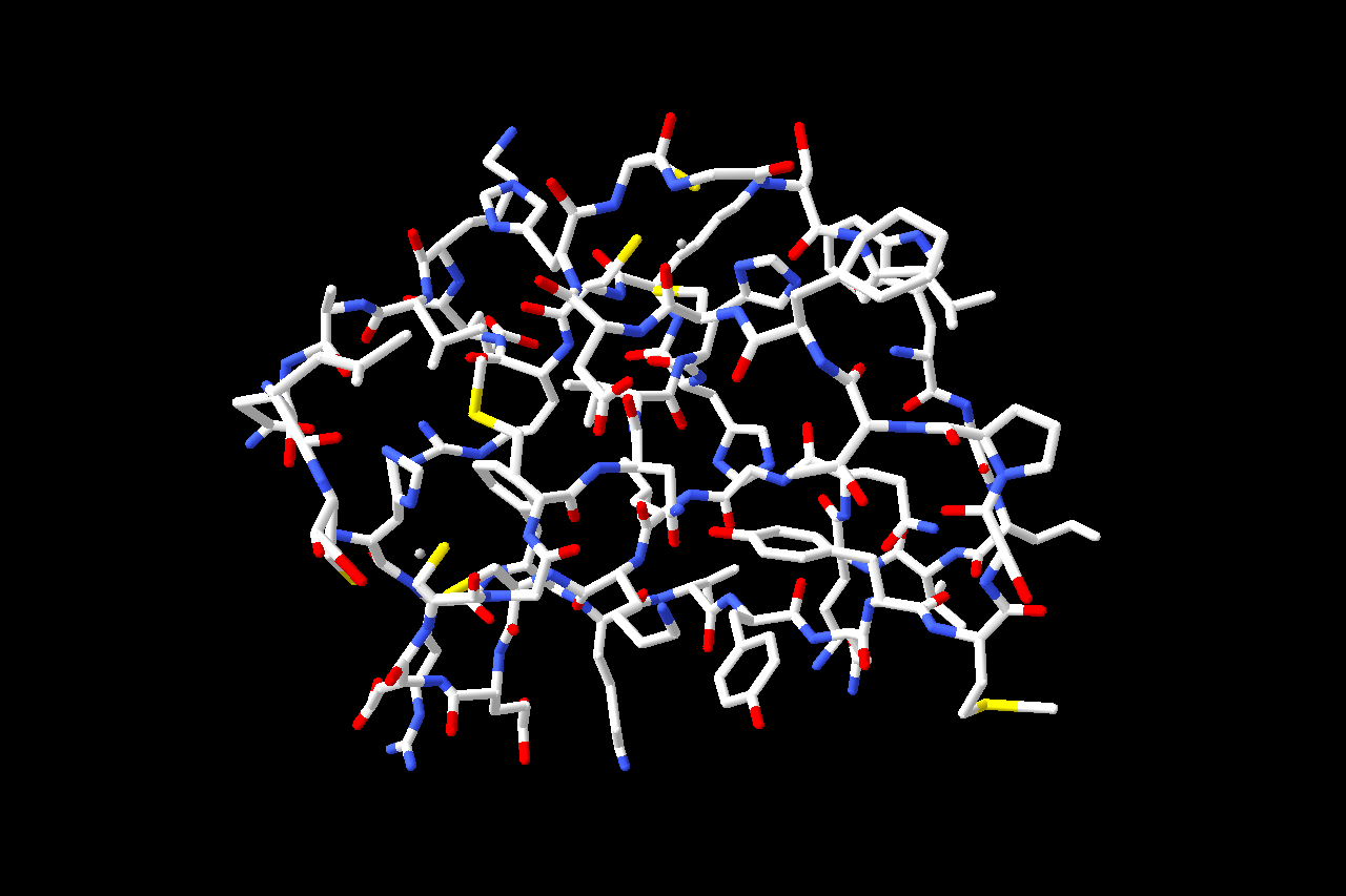
(d) 2,000 steps, -51 dB.

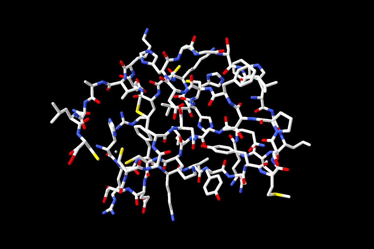
(e) 5,000 steps, -84 dB.

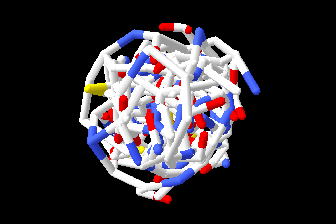
(f) 500 steps, -22 dB.

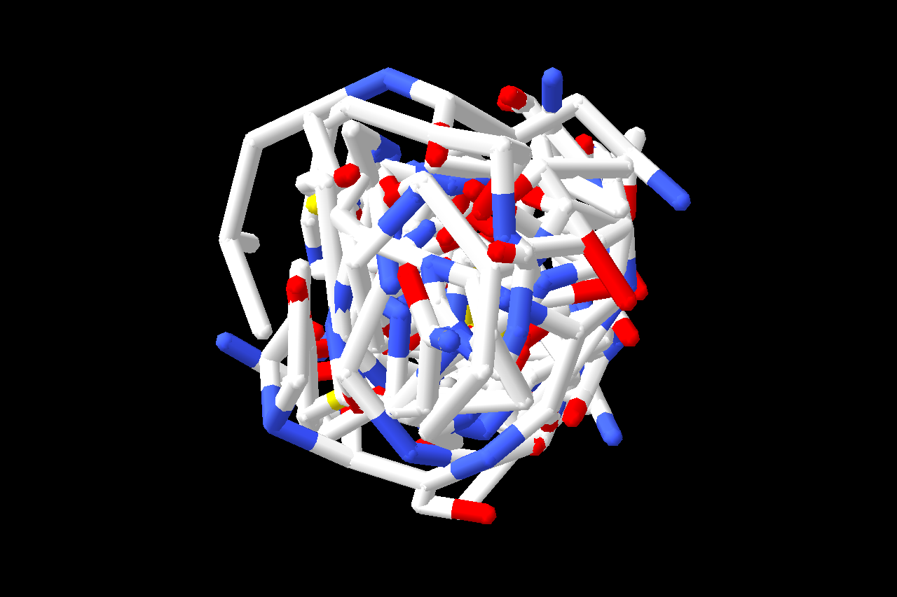
(g) 1,000 steps, -24 dB.

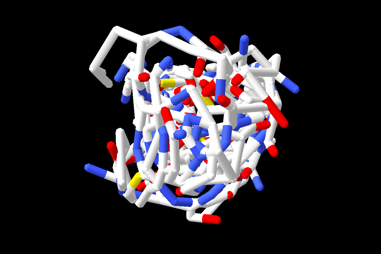
(h) 1,500 steps, -25 dB.

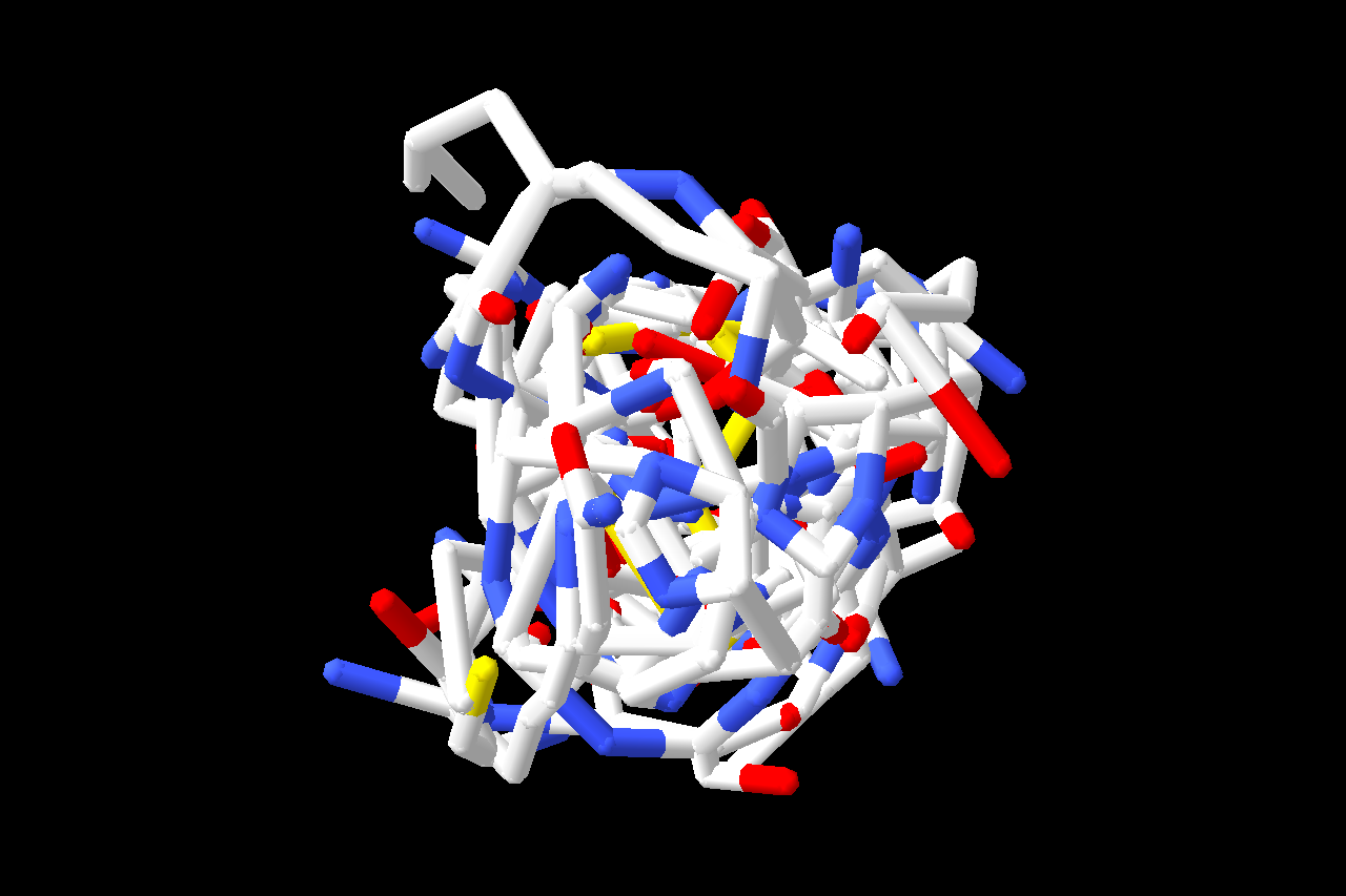
(i) 2,000 steps, -25 dB.

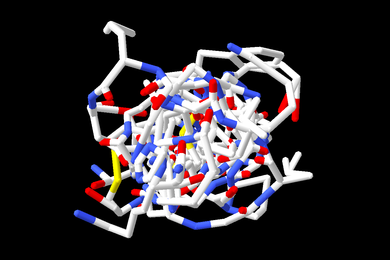
(j) 5,000 steps, -28 dB.

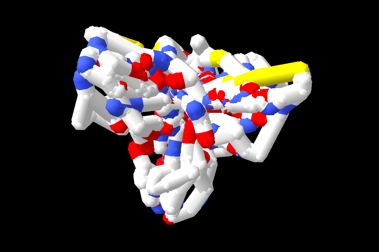
(k) Before.

(l) Original.

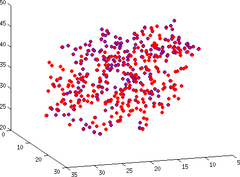
(m) Atom positions.

Figure 2: Reconstructions (displayed in Swiss-PdbViewer) of the protein 1PTQ obtained from the Douglas–Rachford algorithm (a)–(e) and from the method of cyclic projections (f)–(j), together with their relative errors after given numbers of steps. The protein prior to the reconstruction is shown in (k) and its actual structure in (l). Only interatomic distances below 6Å have been used as input. This represents 14,370/162,812 distances (i.e. 8.83% of the nonzero entries of the distance matrix). Entry (m) shows the positions of the original (resp. reconstructed) atoms in red (resp. blue) – coincidence is frequent.

Figure 3: The five proteins not shown in Figure 2. The first column shows positions of original (resp. reconstructed) atom in red (resp. blue), the second and third columns show the original protein and a reconstructioned instance (displayed in Swiss-PdbViewer), as reported in Table 1.

Protein	Atom positions	Original	Reconstruction
1HOE
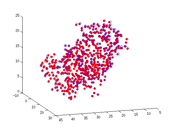
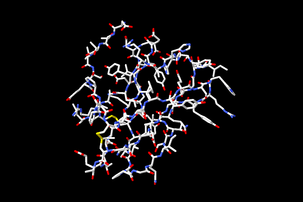
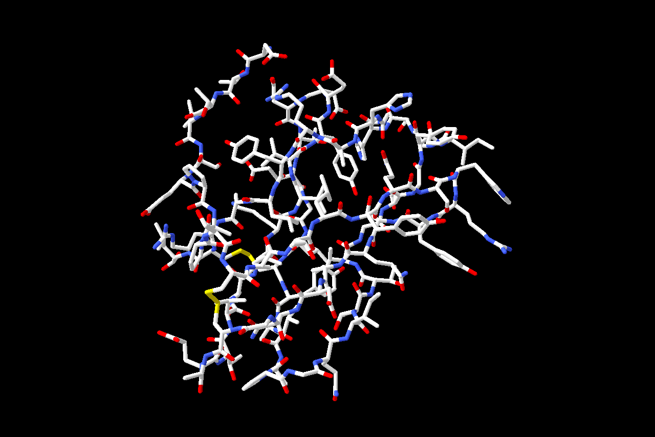
1LFB
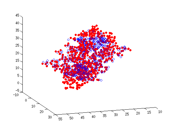
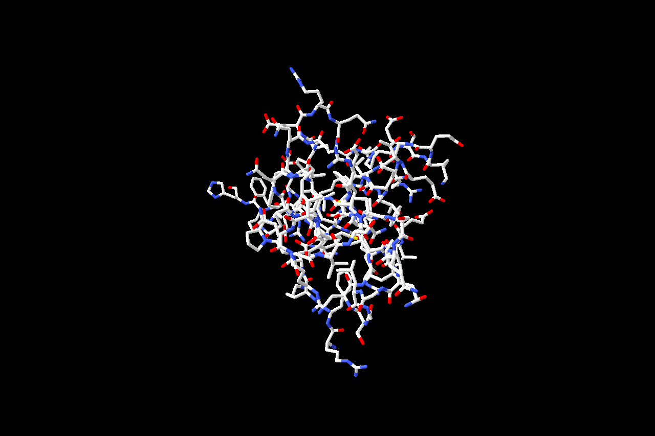
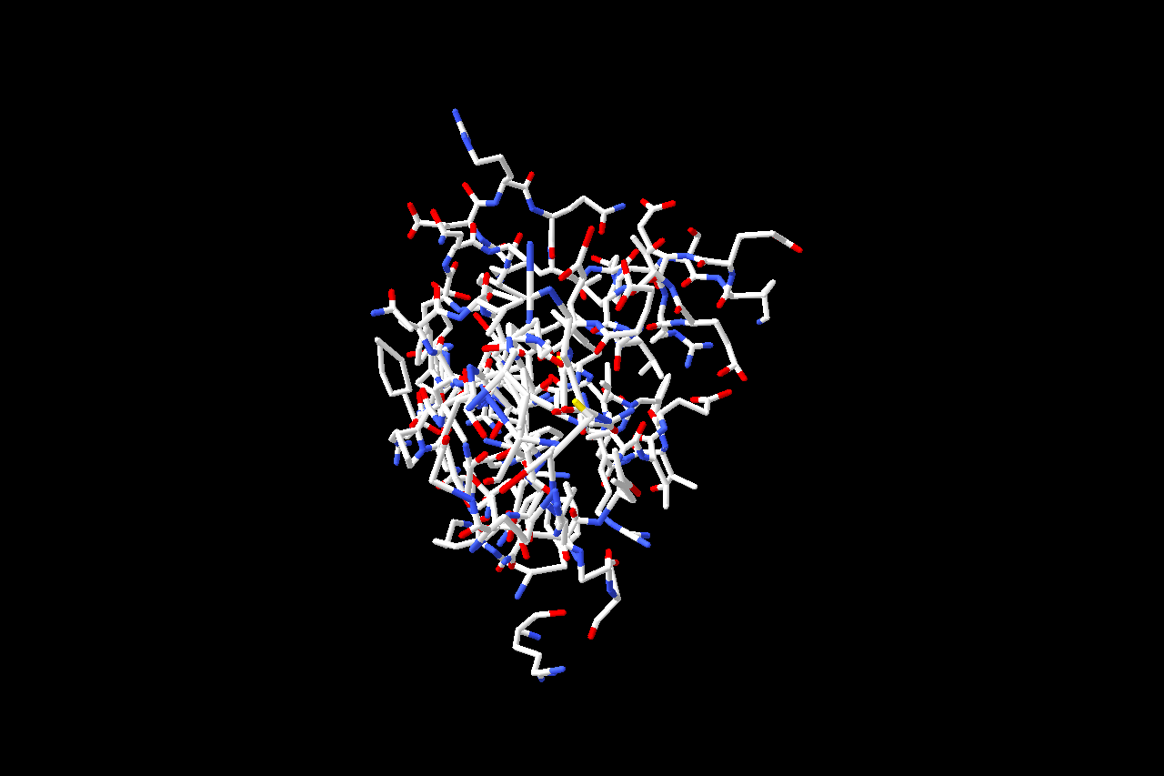
1PHT
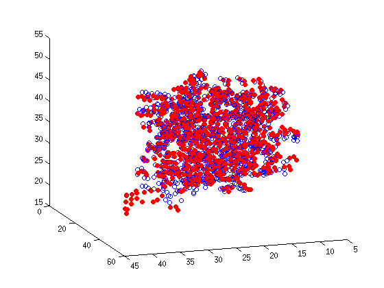
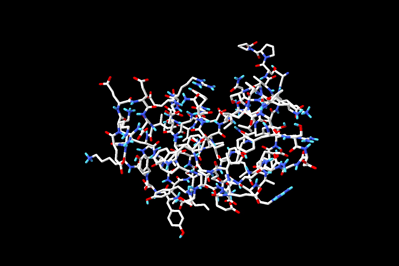
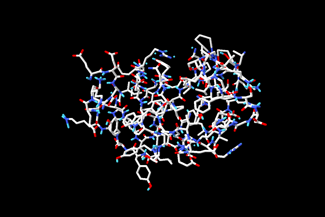
1POA
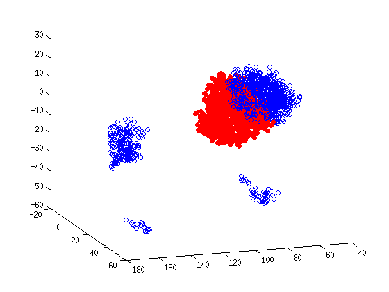
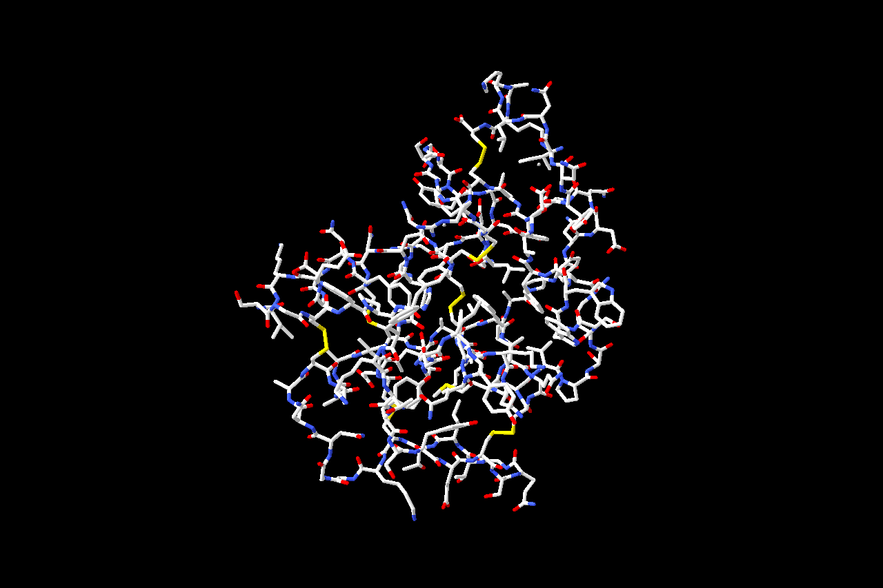
1AX8

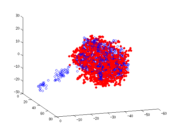
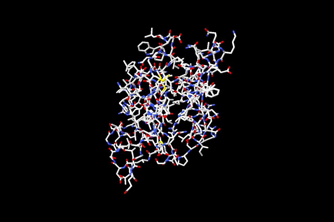
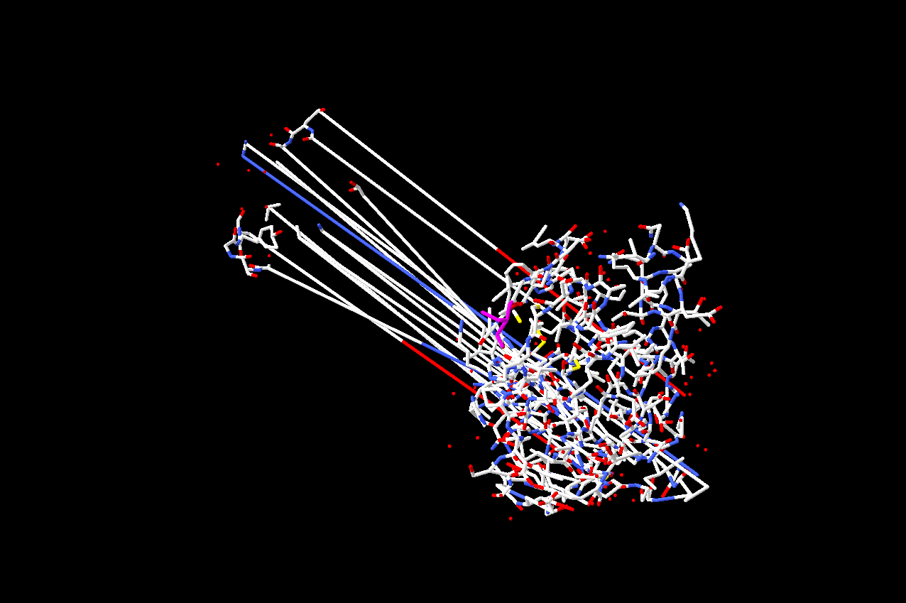
Remark 4.1 (An upper bound on distances).

The constraint $C_{1}$ can be easily modified to incorporate additional distance information. For instance, upper and lower bounds could be placed on the distance between (not necessarily adjacent) carbons atoms on a carbon chain. Note that each carbon-carbon bond is approximately 1.5Å in length. $\Diamond$

Remark 4.2 (Two phase approach).

In our implementation, the Douglas–Rachford method encountered difficulties applied to the reconstruction of the two larger proteins. It therefore would be reasonable to consider an approach were one partitions the atoms into sets and applies the Douglas–Rachford to these sub-problems. The reconstructed distances obtained from these sub-problems can then be used as the initial estimates for distances in the original master problem (which considers all the atoms). An iterative version is outline in Algorithm 4.

input : $D\in\mathbb{R}^{n\times n}$ (the partial Euclidean distances matrix)

Choose random $X\in[-1,1]^{n\times n}$;

$\Gamma:=\{1,2,\dots,n\}$ (each index represents an atom);

while continue do

       if doPhase1 then // generate and solve sub-problems (phase 1)

             Choose a partition of $\Gamma$ into the sets $\Gamma_{1},\Gamma_{2},\dots,\Gamma_{m}$;

             for $k=1,2,\dots,m$ do

                   Apply Algorithm 2 to atoms indexed by $\Gamma_{k}$ to obtain $X_{k}$ (i.e. the distance matrix for the atoms indexed by $\Gamma_{k}$).;

                   Update $X$ with the reconstructed distances in $X_{k}$;

                  

             end for

            

      else // solve master problem (phase 2)

             Apply Algorithm 2 to all atoms (i.e. index by $\Gamma$) to obtain $X$;

            

       end if

      

end while

output : $X$ (the reconstructed distance matrix)

Algorithm 4 A two phase algorithms for protein reconstruction.

We continue to work on such problem-specific refinements of the Douglas-Rachford method: in most of our example problems a natural splitting is less accessible. $\Diamond$

It would also be interesting to apply the methods of this section to sensor network localization problems requiring the reconstruction of an incomplete distance matrix. See, for example, [21, 35, 25].

4.4 Hadamard matrices

Recall that a matrix $H=(H_{ij})\in\{-1,1\}^{n\times n}$ is said to be a Hadamard matrix of order $n$ if

$$H^{T}H=nI.$$ (23)

We note that there are many equivalent characterizations. For instance, (23) is equivalent to asserting that $H$ has maximal determinant (i.e. $|\det H|=n^{n/2}$) [31, Chapter 2]. A classical result of Hadamard asserts that Hadamard matrices exist only if $n=1,2$ or a multiple of $4$. For orders $1$ and $2$, such matrices are easy to find. For multiples of $4$, the Hadamard conjecture asks the converse: If $n$ is a multiple of $4$, does there exists a Hadamard matrix of order $n$? Background on Hadamard matrices can be found in [31]. Thus, an important completion problem starts with structure restrictions, but with no fixed entries.

Consider the now the problem of finding a Hadamard matrix of a given order. We define the constraints:

$$C_{1} :=\{X\in\mathbb{R}^{n\times n}|X_{ij}=\pm 1\text{ for }i,j=1,\dots,n\},$$ (24)

$$C_{2} :=\{X\in\mathbb{R}^{n\times n}|X^{T}X=nI\}.$$ (25)

Then $X$ is a Hadamard matrix if and only if $X\in C_{1}\cap C_{2}$.

The first constraint, $C_{1}$, is clearly non-convex. However, its projection is simple and is given pointwise by

$$P_{C_{1}}(X)_{ij}=\left\{\begin{array}[]{cl}-1&\text{if }X_{ij}<-1,\\ \pm 1&\text{if }X_{ij}=0,\\ 1&\text{otherwise.}\end{array}\right.$$ (26)

The second constraint, $C_{2}$, is also non-convex. To see this, consider the mid-point of the two matrices

$$\begin{pmatrix}\sqrt{2}&0\\ 0&\sqrt{2}\\ \end{pmatrix},\begin{pmatrix}0&\sqrt{2}\\ \sqrt{2}&0\\ \end{pmatrix}\in C_{2}.$$

Nevertheless, a projection can be found by solving the equivalent problem of finding a nearest orthogonal matrix — a special case of the Procrustes problem described above.

Proposition 4.1.

Let $X=USV^{T}$ be a singular value decomposition. Then

$$\sqrt{n}UV^{T}\in P_{C_{2}}(X).$$

Proof.

Let $Y=X/\sqrt{n}$. Then

$$\min_{X\in\mathbb{R}^{n\times n}\atop A^{T}A=nI}\|X-A\|_{F}=\sqrt{n}\left(\min_{Y\in\mathbb{R}^{n\times n}\atop B^{T}B=I}\|Y-B\|_{F}\right).$$

Any solution to the latter is the nearest orthogonal matrix to $Y$. One such matrix can be obtained by replacing all singular values of $Y$ by ‘one’ (see, for example, [41]). Since

$$Y=U\hat{S}V^{T}\text{ where }\hat{S}=S/\sqrt{n},$$

is a singular value decomposition, it follows that $UV$ is the nearest orthogonal matrix to $Y$. The result now follows. ∎

Remark 4.3.

Any $A\in P_{C_{2}}(X)$ is such that $\operatorname{tr}(A^{T}X)=\max_{B\in C_{2}}\operatorname{tr}(B^{T}X)$. $\Diamond$

Remark 4.4.

Consider instead the matrix completion problem of finding a Hadamard matrix with some known entries. This can be cast within the above framework by appropriate modification of $C_{1}$. The projection onto $C_{1}$ only differs by leaving the known entries unchanged. $\Diamond$

We next give a second useful formulation for the problem of finding a Hadamard matrix of a given order. We take $C_{1}$ as in (23) and define

$$C_{3}:=\{X\in\mathbb{R}^{n\times n}|X^{T}X=\|X\|_{F}\,I\}.$$

If $X\in C_{1}$ then $\|X\|_{F}=n$, hence $C_{1}\cap C_{2}=C_{1}\cap C_{3}$. It follows that $X$ is a Hadamard matrix if and only if $X\in C_{1}\cap C_{3}$. A projection onto $C_{3}$ is given similarly $P_{C_{2}}$.

Proposition 4.2.

Let $X=USV^{T}$ be a singular value decomposition. Then

$$\sqrt{\|X\|_{F}}\,UV^{T}\in P_{C_{3}}(X).$$

Proof.

This is a straightforward modification of Proposition 4.1. ∎

Remark 4.5 (Complex Hadamard matrices).

It is also possible to consider complex Hadamard matrices. In this case,

$$C_{1}:=\{X\in\mathbb{C}^{n\times n}|~{}|X_{ij}|=1\}.$$

The projection onto $C_{1}$ is straightforward, and is given by

$$P_{C_{1}}(X)_{ij}=\left\{\begin{array}[]{cl}X_{ij}/|X_{ij}|&\text{if }X_{ij}\neq 0,\\ C_{1}&\text{otherwise.}\\ \end{array}\right.$$

Note that the real solutions to $|X_{ij}|=1$ are $\pm 1$.$\Diamond$

Example 4.1 (Experiments with Hadamard matrices).

Let $H_{1}$ and $H_{2}$ be Hadamard matrices. We say $H_{1}$ are $H_{2}$ are distinct if $H_{1}\neq H_{2}$. We say $H_{1}$ and $H_{2}$ are equivalent if $H_{2}$ can be obtained from $H_{1}$ by performing a sequence of row/column permutations, and/or multiplying row/columns by $-1$. The number of distinct (resp. inequivalent) Hadamard matrices of order $4n$ is given in OEIS sequence A206712 :768, 4954521600, 20251509535014912000,… (resp. A00729: 1, 1, 1, 1, 5, 3, 60, 487, 13710027, …). With increasing order, the number of Hadamard matrices is a faster than exponentially decreasing proportion of the total number of $\{+1,-1\}$-matrices (of which there are $2^{n^{2}}$ for order $n$). This is reflected in the observed rapid increase in difficulty of finding Hadamard matrices using the Douglas–Rachford scheme, as order increases.

We applied the Douglas–Rachford algorithm to 1000 random replications, for each of the above formulation. Our computational experience is summarized in Table 2 and Figure 4. To determine if two Hadamard matrices are equivalent, we use a Sage implementation of the graph isomorphism approach outlined in [38].

Table 2: Number of Hadamard matrices found from 1000 instances.

Order	Prop. 4.1 Formulation				Prop. 4.2 Formulation
	Ave Time (s)	Solved	Distinct	Inequivalent	Ave Time (s)	Solved	Distinct	Inequivalent
2	1.1371	534	8	1	1.1970	505	8	1
4	1.0791	627	422	1	0.2647	921	541	1
8	0.7368	996	996	1	0.0117	1000	1000	1
12	7.1298	0	0	0	0.8337	1000	1000	1
16	9.4228	0	0	0	11.7096	16	16	4
20	20.6674	0	0	0	22.6034	0	0	0

We make some brief comments our the results.

• The formulation based on Proposition 4.2 was found to be faster and more successful than the formulation based on Proposition 4.1, especially for orders $8$ and $12$ where it was successful in every replication. For order less than or equal to 12, the Douglas–Rachford schema was able to find the unique inequivalent Hadamard matrix under either formulation (except for $n=12$, Prop. 4.1 formulation). Moreover, the Proposition 4.2 formulation was able to find four of the five inequivalent Hadamard matrices of order 16.

• From Figure 4 we observe that if a Hadamard matrix was found, it was usually found within the first few thousand iterations. The frequency histogram for order 16, shown in Figure 4(f), varied significantly from the corresponding histograms for lower orders.

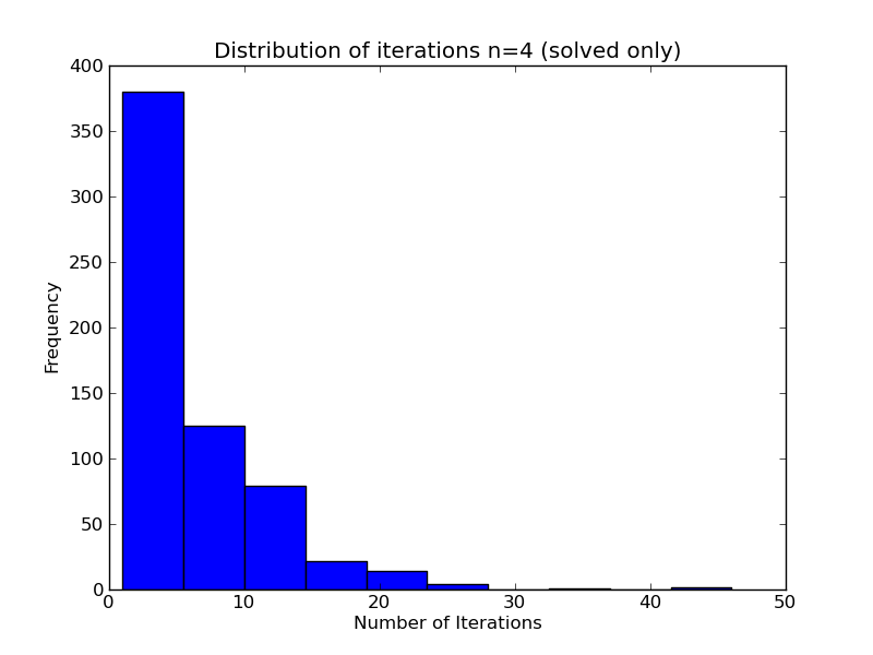
(a) $n=4$, Prop. 4.1 formulation.

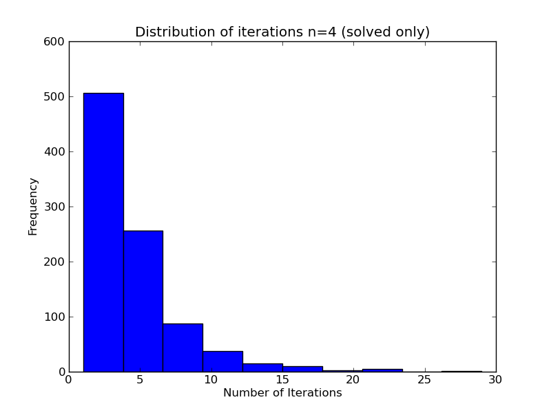
(b) $n=4$, Prop. 4.2 formulation.

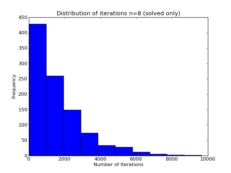
(c) $n=8$, Prop. 4.1 formulation.

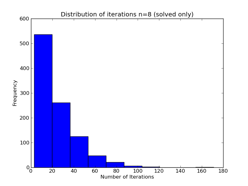
(d) $n=8$, Prop. 4.2 formulation.

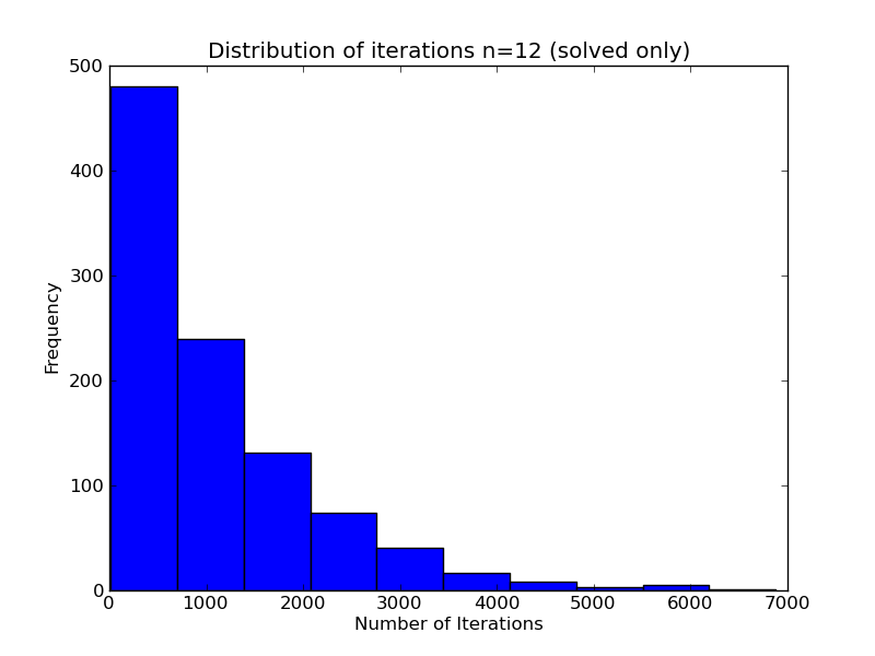
(e) $n=12$, Prop. 4.2 formulation.

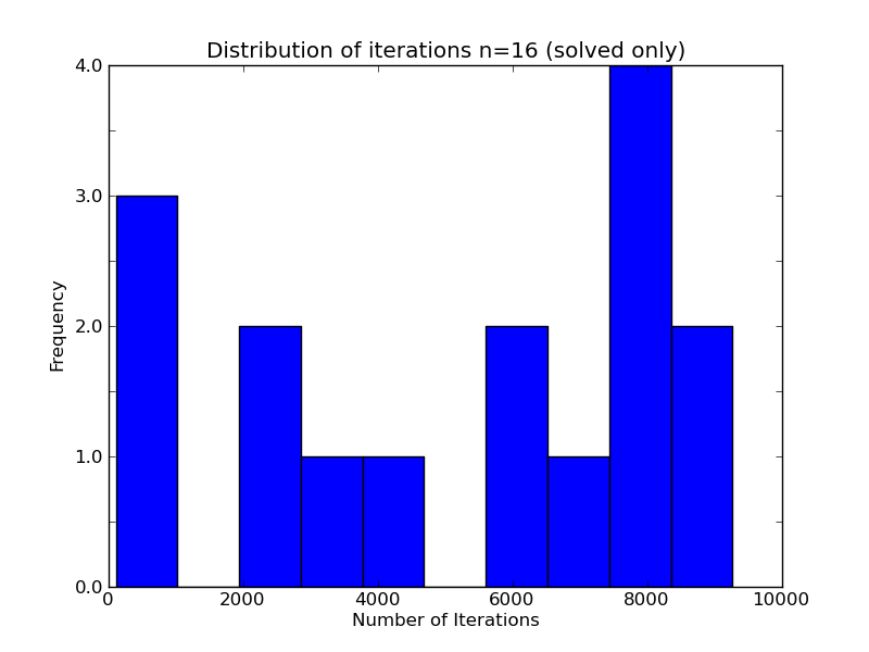
(f) $n=16$, Prop. 4.2 formulation.

Figure 4: Frequency histograms showing the number of iterations required to find a Hadamard matrix, for different order and formulations (solved instances only).

For orders 20 and above, it is possible that another formulation might be more fruitful, but almost certainly better and more problem-specific heuristics will again be needed. $\Diamond$

Remark 4.6.

Since $C_{2}$ is non-convex, when computing its projection we are forced to make a selection from the set of nearest points. In our experiments we have always chosen the nearest point in the same way. It maybe possible to benefit from making the selection according to some other criterion. $\Diamond$

We now turn our attention to some special classes of Hadamard matrices.

4.4.1 Skew-Hadamard matrices

Recall that a matrix $A=(a_{ij})\in\mathbb{R}^{n\times n}$ is skew-symmetric if $A^{T}=-A$. A skew-Hadamard matrix is a Hadamard matrix, $H$, such that $(I-H)$ is skew-symmetric. That is,

$$H+H^{T}=2I.$$

Skew-Hadamard matrices are of interest, for example, in the construction of combinatorial designs. (For a survey see [34].) The number of inequivalent skew-Hadamard matrices of order $4n$ is given in OEIS sequence A001119: 1, 1, 2, 2, 16, 54, …(for $n=2,3,\dots$).

In addition to the constraints $C_{1}$ and $C_{2}$ from the previous section, we define the affine constraint

$$C_{3}:=\{X\in\mathbb{R}^{n\times n}|X+X^{T}=2I\}.$$

A projection onto $C_{1}\cap C_{3}$ is given by

$$P_{C_{1}\cap C_{3}}(X)_{ij}=\left\{\begin{array}[]{cl}1&\text{if }i\neq j\text{ and }X_{ij}\geq X_{ji},\\ -1&\text{if }i\neq j\text{ and }X_{ij}<X_{ji},\\ 1&\text{otherwise.}\end{array}\right.$$

Then $X$ is a skew-Hadamard matrix if and only if $X\in(C_{1}\cap C_{3})\cap C_{2}$.

Table 3 shows the results of the same experiment as Section 4.4, but with the skew constraint incorporated.

Table 3: Number of skew-Hadamard matrices found from 1000 instances.

Order	Prop. 4.1 Formulation				Prop. 4.2 Formulation
	Ave Time (s)	Solved	Distinct	Inequivalent	Ave Time (s)	Solved	Distinct	Inequivalent
2	0.0003	1000	2	1	0.0004	1000	2	1
4	1.1095	719	16	1	1.6381	634	16	1
8	0.7039	902	889	1	0.0991	986	968	1
12	14.1835	43	43	1	0.0497	999	999	1
16	19.3462	0	0	0	0.2298	1000	1000	2
20	29.0383	0	0	0	20.0296	495	495	2

Remark 4.7.

Comparing the results of Table 3 with those of Table 2, it is notable that by placing additional constraints on the problem, both methods now succeed at higher orders, method two is faster than before, and we can successfully find all inequivalent skew matrices of order 20 or less.

In contrast, the three-set feasibility problem $C_{1}\cap C_{2}\cap C_{3}$ was unsuccessful, except for order 2. This is despite the projection onto the affine set $C_{3}$ having the simple formula

$$P_{C_{3}}(X)=I+\frac{X-X^{T}}{2}.$$ (27)

Many mysteries remain! $\Diamond$

4.4.2 Circulant Hadamard matrices

Recall that a matrix $A=(a_{ij})\in\mathbb{R}^{n\times n}$ is circulant if it can be expressed as

$$A=\begin{pmatrix}\lambda_{1}&\lambda_{2}&\dots&\lambda_{n}\\ \lambda_{n}&\lambda_{1}&\dots&\lambda_{n-1}\\ \vdots&\vdots&\ddots&\vdots\\ \lambda_{2}&\lambda_{3}&\dots&\lambda_{1}\\ \end{pmatrix}$$

for some vector $\lambda\in\mathbb{R}^{n}$.

The set of circulant matrices form a subspace of $\mathbb{R}^{n\times n}$. The set $\{P^{k}:i=1,2,\dots,n\}$, where $P$ is the cyclic permutation matrix

$$P:=\begin{pmatrix}0&0&\dots&0&1\\ 1&0&\dots&0&0\\ \vdots&\vdots&\ddots&\vdots&\vdots\\ 0&0&\dots&1&0\\ \end{pmatrix},$$

forms a basis. Consequently, any circulant matrix, $A$, can be expressed as the linear combination of the form

$$A=\sum_{k=1}^{n}\lambda_{k}P^{k}.$$

Remark 4.8.

Right (resp. left) multiplication by $P$ results in a cyclic permutation of rows (resp. columns). Hence $P^{2},P^{3},\dots,P^{n}$ represent all cyclic permutations of the rows (resp. columns) of $P$. In particular, $P^{n}$ is the identity matrix. $\Diamond$

Proposition 4.3 ([30, Ex. 6.7]).

For $X\in\mathbb{R}^{n\times n}$, the nearest circulant matrix is given by

$$\sum_{k=1}^{n}\lambda_{k}P^{k}\text{ where }\lambda_{k}=\frac{1}{n}\sum_{i,j}P^{k}_{ij}X_{ij}.$$

A circulant Hadamard matrix is a Hadamard matrix which is also circulant.

The circulant Hadamard conjecture asserts: No circulant Hadamard matrix of order larger than $4$ exists. For recent progress on the conjecture, see [37]. Consistent with this conjecture, our Douglas–Rachford implementation can successfully find circulant matrices of order 4, but fails for higher orders.

5 Conclusion

We have provided general guidelines for successful application of the Douglas Rachford method to (real) matrix completion problems: both convex and non-convex. The message of the previous two sections is the following. When presented with a new (potentially non-convex) feasibility problem it is well worth seeing if Douglas–Rachford can deal with it— as it is both conceptually very simple and is usually relatively easy to implement. If it works one may then think about refinements if performance is less than desired.

Moreover, this approach allows for the intuition developed for continuous optimization in Euclidean space to be usefully repurposed. This also lets one profitably consider non-expansive fixed point methods in the class of so-called CAT(0) metric spaces — a far ranging concept introduced twenty years ago in algebraic topology but now finding applications to optimization and fixed point algorithms. The convergence of various projection type algorithms to feasible points is under investigation by Searston and Sims among others in such spaces [12] — thereby broadening the constraint structures to which projection-type algorithms apply to include metrically rather than only algebraically convex sets.

Future computational experiments could include:

• Implementing the modifications to the protein reconstruction formulation outlined in Remarks 4.1 and 4.2.

• Consideration of similar reconstruction problems arising in the context of ionic liquid chemistry, and as mentioned, sensor location problems.

• Likewise, for the discovery of larger Hadamard matrices to be tractable by Douglas–Rachford methods, a more efficient implementation is needed and a more puissant model.

Acknowledgments

We wish to thank Judy-anne Osborn and Richard Brent for useful discussions about Hadamard matrices, David Allingham for useful discussions on correlation matrices, Henry Wolkowicz for directing us to many useful matrix completion resources, and Brailey Sims for careful reading of the manuscript.

Many resources can be found at the paper’s companion website:

http://carma.newcastle.edu.au/DRmethods

References

- [1] D. Allingham and J.C.W. Rayner.: Testing equality of corresponding variances for two multivariate samples. In preparation (2013).
- [2] G. Ammar, P. Benner and V. Mehrmann.: A multishift algorithm for the numerical solution of algebraic Riccati equations. Electron. Transactions on Numer. Anal. 1, 33–48 (1993).
- [3] F.J. Aragón Artacho and J.M. Borwein.: Global convergence of a non-convex Douglas–Rachford iteration. J. Glob. Optim. 1–17 (2012). doi: 10.1007/s10898-012-9958-4.
- [4] F.J. Aragón Aracho, J.M. Borwein and M.K. Tam.: Recent results on Douglas–Rachford method for combinatorial optimization problems. Preprint http://arxiv.org/abs/1305.2657 (2013).
- [5] H.H. Bauschke and J.M. Borwein.: On the convergence of von Neumann’s alternating projection algorithm for two sets. Set-Valued Analysis 1(2), 185–212 (1993).
- [6] H.H. Bauschke and J.M. Borwein.: Dykstra’s alternating projection algorithm for two sets. J. Approx. Theory 79(3), 418–443 (1994).
- [7] H.H. Bauschke and J.M. Borwein.: On projection algorithms for solving convex feasibility problems. SIAM Rev. 38, 367–426 (1996).
- [8] H.H. Bauschke, J.M. Borwein and A. Lewis.: The method of cyclic projections for closed convex sets in Hilbert space. Contemp. Math. 204, 1–38 (1997).
- [9] H.H. Bauschke, P.L. Combettes and D.R. Luke.: Phase retrieval, error reduction algorithm, and Fienup variants: a view from convex optimization. J. Opt. Soc. Am. A. 19(7), 1334-1345 (2002).
- [10] H.H. Bauschke, P.L. Combettes and D.R. Luke.: Hybrid projection–reflection method for phased retrieval. J. Opt. Soc. Am. A. 20(6), 1025-1034 (2003).
- [11] H.H. Bauschke, P.L. Combettes and D.R. Luke.: Finding best approximation pairs relative to two closed convex sets in Hilbert space. J. Approx. Theory 127(2), 178–192 (2004).
- [12] M. Bačák, M., I. Searston, I., B. Sims.: Alternating projections in CAT(0) spaces. J. Math. Analysis and Appl. 385(2), 599–607 (2012).
- [13] E.G. Birgin and M. Raydan.: Robust stopping criteria for Dykstra’s algorithm. SIAM J. Sci. Comput. 26(4), 1405–1414 (2005).
- [14] J.M. Borwein and A.S. Lewis.: Convex analysis and nonlinear optimization. Springer (2006).
- [15] J.M. Borwein and D.R. Luke.: Entropic regularization of the function. In: Fixed-Point Algorithms for Inverse Problems in Science and Engineering, pp. 65–92. Springer (2011).
- [16] J.M. Borwein and B. Sims.: The Douglas–Rachford algorithm in the absence of convexity. In: Fixed-Point Algorithms for Inverse Problems in Science and Engineering, pp. 93–109. Springer (2011).
- [17] J.M. Borwein and M.K. Tam.: A cyclic Douglas-Rachford iteration scheme. J. Optim. Theory Appl. (2013). doi: 10.1007/s10957-013-0381-x
- [18] S.P. Boyd and L. Vandenberghe.: Convex Optimization. Cambridge University Press (2004).
- [19] J. Boyle and R. Dykstra.: A method for finding projections onto the intersection of convex sets in Hilbert spaces. Lecture Notes in Statistics 37, 28-47 (1986).
- [20] Y. Chen and X. Ye.: Projection onto a simplex. http://arxiv.org/abs/1101.6081v2 (2011).
- [21] P. Drineas, A. Javed, M. Magdon-Ismail, G. Pandurangant, R. Virrankoski, and A. Savvides.: Distance matrix reconstruction from incomplete distance information for sensor network localization. Proc. of the IEEE Int. Conf. on Sens. and Ad Hoc Commun. and Netw. (SECON’06) 2, 536–544 (2006).
- [22] R. Escalante and M. Raydan.: Alternating projection methods. SIAM (2011).
- [23] L. Fabry-Asztalos, I. Lorentz and R. Andonie.: Molecular distance geometry optimization using geometric build-up and evolutionary techniques on GPU. Comput. Intell. in Bioinforma. and Comput. Biol. 321–328 (2012).
- [24] N. Gaffke and R. Mathar.: A cyclic projection algorithm via duality. Metrika 36, 29–54 (1989).
- [25] M.R. Gholami, L. Tetruashvili, E.G. Ström and Y. Censor.: Cooperative wireless sensor network positioning via implicit convex feasibility. IEEE Transactions on Signal Process. (2013).
- [26] W Glunt, T.L. Hayden, S. Hong, and J. Wells.: An alternating projection algorithm for computing the nearest Euclidean distance matrix SIAM J. Matrix Anal. Appl. 11(4), 589–600 (1990).
- [27] T.L. Hayden and J. Wells.: Approximation by matrices positive semidefinite on a subspace Linear Algebra Appl. 109, 115–130 (1988).
- [28] R. Hesse and D.R. Luke.: Nonconvex notions of regularity and convergence of fundamental algorithms for feasibility problems. Preprint http://arxiv.org/abs/1212.3349 (2012).
- [29] N.J. Higham.: Computing the polar decomposition—with applications. SIAM J. Sci. Stat. Comput. 7(4), 1160–1174 (1986).
- [30] A. Hjørungnes.: Complex-valued matrix derivatives: with applications in signal processing and communications. Cambridge University Press (2011).
- [31] K.J. Horadam.: Hadamard Matrices and their Applications. Princeton University Press (2007).
- [32] R.A. Horn and C.R. Johnson.: Matrix analysis Cambridge University Press (1985).
- [33] C.R. Johnson. Matrix completion problems: a survey.: Proc. of Sympos. in App. Math. 40, 171–198 (1990).
- [34] C. Koukouvinos and S. Stylianou.: On skew-Hadamard matrices. Discret. Math. 309, 2723–2731 (2008).
- [35] N. Kirslock and H. Wolkowicz.: Explicity sensor network localization using semidefinite representations and facial reductions. SIAM J. Optim. 20(5), 2679–2708 (2010).
- [36] M. Laurent.: Matrix completion problems. Encycl. of Optim. 3, 221–229 (2001).
- [37] K.H. Leung and B. Schmidt.: New restrictions on possible order of circulant Hadamard matrices. Des. Codes Cryptorgr. 64, 143–151 (2012).
- [38] B.D. McKay.: Hadamard equivalence via graph isomorphism. Discret. Math. 27(2), 213–214 (1997).
- [39] J. Piantadosi, P. Howlett and J.M. Borwein.: A checkerboard copula to simulate seasonal rainfall. Revision submitted Journal of Hydrology (2013).
- [40] I.J. Schoenberg.: Remarks to Maurice Fréchet’s Article “Sur la définition axiomatique d’une classe d’Espace distanciés vectoriellement applicable sur l’espace de Hilbert” Ann. Math. 36(3), 724–732 (1935).
- [41] P.H. Schönemann.: A generalized solution to the orthogonal Procrustes problem. Psychometrika 31, 1–10 (1966).
- [42] A.K. Yuen, O. Lafon O, T. Charpentier, M. Roy, F. Brunet, P. Berthault, D. Sakellariou, B. Robert, S. Rimsky, F. Pillon, J.C. Cintrat, B. Rousseau.: Measurement of long-range interatomic distances by solid-state tritium-NMR spectroscopy. J. Am. Chem. Soc. 132(6), 1734–1735 (2010).