Generalized Perron–Frobenius Theorem for Nonsquare Matrices

Abstract

The celebrated Perron–Frobenius (PF) theorem is stated for irreducible nonnegative square matrices, and provides a simple characterization of their eigenvectors and eigenvalues. The importance of this theorem stems from the fact that eigenvalue problems on such matrices arise in many fields of science and engineering, including dynamical systems theory, economics, statistics and optimization. However, many real-life scenarios give rise to nonsquare matrices. Despite the extensive development of spectral theories for nonnegative matrices, the applicability of such theories to non-convex optimization problems is not clear. In particular, a natural question is whether the PF Theorem (along with its applications) can be generalized to a nonsquare setting. Our paper provides a generalization of the PF Theorem to nonsquare matrices. The extension can be interpreted as representing client-server systems with additional degrees of freedom, where each client may choose between multiple servers that can cooperate in serving it (while potentially interfering with other clients). This formulation is motivated by applications to power control in wireless networks, economics and others, all of which extend known examples for the use of the original PF Theorem.

We show that the option of cooperation between servers does not improve the situation, in the sense that in the optimal solution no cooperation is needed, and only one server needs to serve each client. Hence, the additional power of having several potential servers per client translates into choosing the best single server and not into sharing the load between the servers in some way, as one might have expected.

The two main contributions of the paper are (i) a generalized PF Theorem that characterizes the optimal solution for a non-convex nonsquare problem, and (ii) an algorithm for finding the optimal solution in polynomial time. Towards achieving those goals, we extend the definitions of irreducibility and largest eigenvalue of square matrices to nonsquare ones in a novel and non-trivial way, which turns out to be necessary and sufficient for our generalized theorem to hold. The analysis performed to characterize the optimal solution uses techniques from a wide range of areas and exploits combinatorial properties of polytopes, graph-theoretic techniques and analytic tools such as spectral properties of nonnegative matrices and root characterization of integer polynomials.

1 Introduction

Motivation and main results.

This paper presents a generalization of the well known Perron–Frobenius (PF) Theorem [15, 27]. As a motivating example, let us consider the Power control problem, one of the most fundamental problems in wireless networks. The input to this problem consists of $n$ receiver-transmitter pairs and their physical locations. All transmitters are set to transmit at the same time with the same frequency, thus causing interference to the other receivers. Therefore, receiving and decoding a message at each receiver depends on the transmitting power of its paired transmitter as well as the power of the rest of the transmitters. If the signal to interference ratio at a receiver, namely, the signal strength received by a receiver divided by the interfering strength of other simultaneous transmissions, is above some reception threshold $\beta$, then the receiver successfully receives the message, otherwise it does not [30]. The power control problem is then to find an optimal power assignment for the transmitters, so as to make the reception threshold $\beta$ as high as possible and ease the decoding process.

As it turns out, this power control problem can be solved elegantly by casting it as an optimization program and using the Perron–Frobenius (PF) Theorem [40]. The theorem can be formulated as dealing with the following optimization problem (where $A\in\mathbb{R}^{n\times n}$):

maximize $$\beta$$ subject to: (1)

$$A\cdot\overline{X}\leq 1/\beta\cdot\overline{X},~{}~{}\displaystyle||\overline{X}||_{1}=1,~{}~{}\displaystyle\overline{X}\geq\overline{0}.$$

Let $\beta^{*}$ denote the optimal solution for Program (1). The Perron–Frobenius (PF) Theorem characterizes the solution to this optimization problem and shows the following:

Theorem 1.1

(PF Theorem, short version, [15, 27]) Let $A$ be an irreducible nonnegative matrix. Then $\beta^{*}=1/\mathit{r}$, where $\mathit{r}\in\mathbb{R}_{>0}$ is the largest eigenvalue of $A$, called the Perron–Frobenius (PF) root of $A$. There exists a unique (eigen-)vector $\mathbf{\overline{P}}>0$, $||\mathbf{\overline{P}}||_{1}=1$, such that $A\cdot\mathbf{\overline{P}}=r\cdot\mathbf{\overline{P}}$, called the Perron vector of $A$. (The pair $(\mathit{r},\mathbf{\overline{P}})$ is hereafter referred to as an eigenpair of $A$.)

Returning to our motivating example, let us consider a more complicated variant of the power control problem, where each receiver has several transmitters that can transmit to it (and only to it) synchronously. Since these transmitters are located at different places, it may conceivably be better to divide the power (or work) among them, to increase the reception threshold at their common receiver. Again, the question concerns finding the best power assignment among all transmitters.

In this paper we extend Program (1) to nonsquare matrices and consider the following extended optimization problem, which in particular captures the multiple transmitters scenario. (Here $A,B\in\mathbb{R}^{n\times m}$, $n\leq m$.)

maximize $$\beta$$ subject to: (2)

$$A\cdot\overline{X}\leq 1/\beta\cdot B\cdot\overline{X},\displaystyle~{}~{}~{}||\overline{X}||_{1}=1,~{}~{}~{}\displaystyle\overline{X}\geq\overline{0}.$$

We interpret the nonsquare matrices $A,B$ as representing some additional freedom given to the system designer. In this setting, each entity (receiver, in the power control example) has several affectors (transmitters, in the example), referred to as its supporters, which can cooperate in serving it and share the workload. In such a general setting, we would like to find the best way to organize the cooperation between the supporters of each entity.

The original problem was defined for a square matrix, so the appearance of eigenvalues in the characterization of its solution seems natural. In contrast, in the generalized setting the situation seems more complex. Our main result is an extension of the PF Theorem to nonsquare matrices and systems that give rise to an optimization problem in the form of (2), with optimal solution $\beta^{*}$.

Theorem 1.2

(Nonsquare PF Theorem, short version) Let $\langle A,B\rangle$ be an irreducible nonnegative system (to be made formal later). Then $\beta^{*}=1/\mathit{r}$, where $\mathit{r}\in\mathbb{R}_{>0}$ is the smallest Perron–Frobenius (PF) root of all ${n\times n}$ square sub-systems (defined formally later). There exists a vector $\mathbf{\overline{P}}\geq 0$ such that $A\cdot\mathbf{\overline{P}}=\mathit{r}\cdot B\cdot\mathbf{\overline{P}}$ and $\mathbf{\overline{P}}$ has $n$ entries greater than 0 and $m-n$ zero entries (referred to as a $\boldsymbol{0^{*}}$ solution).

In other words, the theorem implies that the option of cooperation does not improve the situation, in the sense that in the optimum solution, no cooperation is needed and only one supporter per entity needs to work. Hence, the additional power of having several potential supporters per entity translates into choosing the best single supporter and not into sharing the load between the supporters in some way, as one might have expected.

As it turns out, the lion’s share of our analysis involves such a characterization of the optimal solution for (the non-convex) problem of Program (2). The main challenge is to show that at the optimum, there exists a solution in which only one supporter per entity is required to work; we call such a solution a $\boldsymbol{0^{*}}$ solution. Namely, the structure that we establish is that the optimal solution for our nonsquare system is in fact the optimal solution of an embedded square PF system. Indeed, to enjoy the benefits of an equivalent square system, one should show that there exists a solution in which only one supporter per entity is required to work. Interestingly, it turned out to be relatively easy to show that there exists an optimal “almost $\boldsymbol{0^{*}}$” solution, in which each entity except at most one has a single active supporter and the remaining entity has at most two active supporters. Despite the presumably large “improvement” of decreasing the number of servers from $m$ to $n+1$, this still leaves us in the frustrating situation of a nonsquare $n\times(n+1)$ system, where no spectral characterization for optimal solutions exists. In order to allow us to characterize the optimal solution using the eigenpair of the best square matrix embedded within the nonsquare system, one must overcome this last hurdle, and reach the “phase transition” point of $n$ servers, in which the system is square. Our main efforts went into showing that the remaining entity, too, can select just one supporter while maintaining optimality, ending with a square $n\times n$ irreducible system where the traditional PF Theorem can be applied. Proving the existence of an optimal $\boldsymbol{0^{*}}$ solution requires techniques from a wide range of areas to come into play and provide a rich understanding of the system on various levels. In particular, the analysis exploits combinatorial properties of polytopes, graph-theoretic techniques and analytic tools such as spectral properties of nonnegative matrices and root characterization of integer polynomials.

In the context of the above example of power control in wireless network with multiple transmitters per receiver, a $\boldsymbol{0^{*}}$ solution means that the best reception threshold is achieved when only a single transmitter transmits to each receiver. Other known applications of the PF Theorem can also be extended in a similar manner. An Example for such applications is the input-output economic model [28]. In this economic model, each industry produces a commodity and buys commodities (raw materials) from other industries. The percentage profit margin of an industry is the ratio of its total income and total expenses (for buying its raw materials). It is required to find a pricing maximizing the ratio of the total income and total expenses of all industries. The extended PF variant of the problem concerns the case where an industry can produce multiple commodities instead of just one. In this example, the same general phenomenon holds: each industry should charge money only for one of the commodities it produces. That is, in the optimal pricing, one commodity per industry has nonzero price, therefore the optimum is a $\boldsymbol{0^{*}}$ solution. For a more detailed discussion of applications, see Sec. 7. In addition, in Sec. 6, we provide a characterization of systems in which a $\boldsymbol{0^{*}}$ solution does not exist.

While in the original setting the PF root and PF vector can be computed in polynomial time, this is not clear in the extended case, since the problem is not convex [6] (and not even log-convex) and there are exponentially many choices in the system even if we know that the optimal solution is $\boldsymbol{0^{*}}$ and each entity has only two supporters to choose from. Our second main contribution is providing a polynomial time algorithm to find $\beta^{*}$ and $\mathbf{\overline{P}}$. The algorithm uses the fact that fixing $\beta$ yields a relaxed problem which is convex (actually it becomes a linear program). This allows us to employ the well known interior point method [6], for testing a specific $\beta$ for feasibility. Hence, the problem reduces to finding the maximum feasible $\beta$, and the algorithm does so by applying binary search on $\beta$. Clearly, the search results in an approximate solution, in fact yielding a fully polynomial time approximation scheme (FPTAS) for program (2). This, however, leaves open the intriguing question of whether program (2) is polynomial. Obtaining an exact optimal $\beta^{*}$, along with an appropriate vector $\mathbf{\overline{P}}$, is thus another challenging aspect of the problem.

A central notion in the generalized PF theorem is the irreducibility of the system. While irreducibility is a well-established concept for square systems, it is less obvious how to define irreducibility for a nonsquare matrix or system as in Program (2). We provide a suitable definition based on the property that every maximal square (legal) subsystem is irreducible, and show that our definition is necessary and sufficient for the theorem to hold. A key tool in our analysis is what we call the constraint graph of the system, whose vertex set is the set on $n$ constraints (one per entity) and whose edges represent direct influence between the constraints. For a square system, irreducibility is equivalent to the constraint graph being strongly connected, but for nonsquare systems the situation is more delicate. Essentially, although the matrices are not square, the notion of constraint graph is well defined and provides a valuable square representation of the nonsquare system (i.e., the adjacency matrix of the graph). In [34, PF_Archive], we also present a polynomial-time algorithm for testing the irreducibility of a given system, which exploits the properties of the constraint graph.

Related work. The PF Theorem establishes the following two important “PF properties” for a nonnegative square matrix $A\in\mathbb{R}^{n\times n}$: (1) the Perron–Frobenius property: $A$ has a maximal nonnegative eigenpair. If in addition the matrix $A$ is irreducible then its maximal eigenvalue is strictly positive, dominant and with a strictly positive eigenvector. Thus nonnegative irreducible matrix $A$ is said to enjoy the strong Perron–Frobenius property [15, 27]. (2) the Collatz–Wielandt property (a.k.a. min-max characterization): the maximal eigenpair is the optimal solution of Program (1) [12, 38].

Matrices with these properties have played an important role in a wide variety of applications. The wide applicability of the PF Theorem, as well as the fact that the necessary and sufficient properties required of a matrix $A$ for the PF properties to hold are still not fully understood, have led to the emergence of many generalizations. We note that whereas all generalizations concern the Perron–Frobenius property, the Collatz–Wielandt property is not always established. The long series of existing PF extensions includes [23, 14, 31, 19, 33, 20, 29, 22]. We next discuss these extensions in comparison to the current work.

Existing PF extensions can be broadly classified into four classes. The first concerns matrices that do not satisfy the irreducibility and nonnegativity requirements. For example, [23, 14] establish the Perron-Frobenius property for almost nonnegative matrices or eventually nonnegative matrices. A second class of generalizations concerns square matrices over different domains. For example, in [31], the PF Theorem was established for complex matrices $A\in\mathbb{C}^{n\times n}$. In the third type of generalization, the linear transformation obtained by applying the nonnegative irreducible matrix $A$ is generalized to a nonlinear mapping [19, 33], a concave mapping [20] or a matrix polynomial mapping [29].

Last, a much less well studied generalization deals with nonsquare matrices, i.e., matrices in $\mathbb{R}^{n\times m}$ for $m\neq n$. Note that when considering a nonsquare system, the notion of eigenvalues requires definition. There are several possible definitions for eigenvalues in nonsquare matrices. One possible setting for this type of generalizations considers a pair of nonsquare “pencil” matrices $A,B\in\mathbb{R}^{n\times m}$, where the term “pencil” refers to the expression $A-\lambda\cdot B$, for $\lambda\in\mathbb{C}$. Of special interest here are the values that reduce the pencil rank, namely, the $\lambda$ values satisfying $(A-\lambda B)\cdot\overline{X}=\overline{0}$ for some nonzero $\overline{X}$. This problem is known as the generalized eigenvalue problem [22, 11, 5, 21], which can be stated as follows: Given matrices $A,B\in\mathbb{R}^{n\times m}$, find a vector $\overline{X}\neq\overline{0}$, $\lambda\in\mathbb{C}$, so that $A\cdot\overline{X}=\lambda B\cdot\overline{X}$. The complex number $\lambda$ is said to be an eigenvalue of $A$ relative to $B$ iff $A\overline{X}=\lambda\cdot B\cdot\overline{X}$ for some nonzero $\overline{X}$ and $\overline{X}$ is called the eigenvector of $A$ relative to $B$. The set of all eigenvalues of $A$ relative to $B$ is called the spectrum of $A$ relative to $B$, denoted by $sp(A_{B})$.

Using the above definition, [22] considered pairs of nonsquare matrices $A,B$ and was the first to characterize the relation between $A$ and $B$ required to establish their PF property, i.e., guarantee that the generalized eigenpair is nonnegative. Essentially, this is done by generalizing the notions of positivity and nonnegativity in the following manner. A matrix $A$ is said to be positive (respectively,nonnegative) with respect to $B$, if $B^{T}\cdot\overline{Y}\geq 0$ implies that $A^{T}\cdot\overline{Y}>0$ (resp., $A^{T}\cdot\overline{Y}\geq 0$). Note that for $B=I$, these definitions coincide with the classical definitions of a positive (resp., nonnegative) matrix. Let $A,B\in\mathbb{R}^{n\times m}$, for $n\geq m$, be such that the rank of $A$ or the rank of $B$ is $n$. It is shown in [22] that if $A$ is positive (resp., nonnegative) with respect to $B$, then the generalized eigenvalue problem $A\cdot\overline{X}=\lambda\cdot B\cdot\overline{X}$ has a discrete and finite spectrum, the eigenvalue with the largest absolute value is real and positive (resp., nonnegative), and the corresponding eigenvector is positive (resp., nonnegative). Observe that under the definition used therein, the cases where $m>n$ (which is the setting studied here) is uninteresting, as the columns of $A-\lambda\cdot B$ are linearly dependent for any real $\lambda$, and hence the spectrum $sp(A_{B})$ is unbounded.

Despite the significance of [22] and its pioneering generalization of the PF Theorem to nonsquare systems, it is not clear what are the applications of such a generalization, and no specific implications are known for the traditional applications of the PF theorem. Moreover, although [22] established the PF property for a class of pairs of nonsquare matrices, the Collatz–Wielandt property, which provides the algorithmic power for the PF Theorem, does not necessarily hold with the spectral definition of [22]. In addition, since no notion of irreducibility was defined in [22], the spectral radius of a nonnegative system (in the sense of the definition of [22]) might be zero, and the corresponding eigenvector might be nonnegative in the strong sense (with some zero coordinates). These degenerations can be handled only by considering irreducible nonnegative matrices, as was done by Frobenius in [15].

In contrast, the goal of the current work is to develop the spectral theory for a pair of nonnegative matrices in a way that is both necessary and sufficient for both the PF property and the Collatz–Wielandt property to hold (allowing the nonsquare system to be of the “same power” as the square systems considered by Perron and Frobenius). Towards this we define the eigenvalues and eigenvectors of pairs of $n\times m$ matrices $A$ and $B$ in a novel manner. Such eigenpair $(\lambda,\overline{X})$ satisfies $A\cdot\overline{X}=\lambda\cdot B\cdot\overline{X}$. In [22], alternative spectral definitions for pairs of nonsquare matrices $A$ and $B$ are provided. We note that whereas in [22] formulation, the maximum eigenvalue is not bounded if $n<m$, with our definition it is bounded.

Let us note that although the generalized eigenvalue problem has been studied for many years, and multiple approaches for nonsquare spectral theory in general have been developed, the algorithmic aspects of such theories with respect to the the Collatz–Wielandt property have been neglected when concerning nonsquare matrices (and also in other extensions). This paper is the first, to the best of our knowledge, to provide spectral definitions for nonsquare systems that have the same algorithmic power as those made for square systems (in the context of the PF Theorem). The extended optimization problem that corresponds to this nonsquare setting is a nonconvex problem (which is also not log-convex), therefore its polynomial solution and characterization are of interest.

Another way to extend the notion of eigenvalues and eigenvectors of a square matrix to a nonsquare matrix is via singular value decompositions (SVD) [25]. Formally, the singular value decomposition of an $n\times m$ real matrix $M$ is a factorization of the form $M=U\Sigma V^{*}$, where $U$ is an $m\times m$ real or complex unitary matrix, $\Sigma$ is an $m\times n$ diagonal matrix with nonnegative reals on the diagonal, and $V^{*}$ (the conjugate transpose of $V$) is an $n\times n$ real or complex unitary matrix. The diagonal entries $\Sigma_{i,i}$ of $\Sigma$ are known as the singular values of $M$. After performing the product $U\Sigma V^{*}$, it is clear that the dependence of the singular values of $M$ is linear. In case all the inputs of $M$ are positive, we can add the absolute value, and thus the SVD has a flavor of $L^{1}$ dependence. In contrast to the SVD definition, here we are interested in finding the maximum, so our interpretation has the flavor of $L^{\infty}$.

In a recent paper [37], Vazirani defined the notion of rational convex programs as problems that have a rational number as a solution. Our paper can be considered as an example for algebraic programming, since we show that a solution to our problem is an algebraic number.

2 Preliminaries

2.1 Definitions and terminology

Consider a directed graph $G=(V,E)$. A subset of the vertices $W\subseteq V$ is called a strongly connected component if $G$ contains a directed path from $v$ to $u$ for every $v,u\in W$. $G$ is said to be strongly connected if $V$ is a strongly connected component.

Let $A\in\mathbb{R}^{n\times n}$ be a square matrix. Let $EigVal(A)=\{\lambda_{1},\ldots,\lambda_{k}\}$, $k\leq n$, be the set of real eigenvalues of $A$. The characteristic polynomial of $A$, denoted by $\mathrm{P}(A,t)$, is a polynomial whose roots are precisely the eigenvalues of $A$, $EigVal(A)$, and it is given by

$$\mathrm{P}(A,t)=\det(t\cdot I-A)$$ (3)

where $I$ is the $n\times n$ identity matrix. Note that $\mathrm{P}(A,t)=0$ iff $t\in EigVal(A)$. The spectral radius of $A$ is defined as $\rho(A)=\displaystyle\max\limits_{\lambda\in EigVal(A)}|\lambda|.$ The $i^{th}$ element of a vector $\overline{X}$ is given by $X(i)$, and the $i,j$ entry of a matrix $A$ is denoted $A(i,j)$. Let $A_{i,0}$ (respectively, $A_{0,i}$) denote the $i$-th row (resp., column) of $A$. Vector and matrix inequalities are interpreted in the component-wise sense. $A$ is positive (respectively, nonnegative) if all its entries are. $A$ is primitive if there exists a natural number $k$ such that $A^{k}>0$. $A$ is irreducible if for every $i,j$, there exists a natural $k_{i,j}$ such that $(A^{k_{i,j}})_{i,j}>0.$ An irreducible matrix $A$ is periodic with period $\mathit{h}$ if $(A^{t})_{ii}=0$ for $t\neq k\cdot\mathit{h}$.

2.2 Algebraic Preliminaries

Generalization of Cramer’s rule to homogeneous linear systems.

Let $A_{i,0}$ (respectively, $A_{0,i}$) denote the $i$-th row (resp., column) of $A$. Let $A_{-(i,j)}$ denote the matrix that results from $A$ by removing the $i$-th row and the $j$-th column. Similarly, $A_{-(i,0)}$ and $A_{-(0,j)}$ denote the matrix after removing the $i$-th row (respectively, $j$-th column) from $A$. Let $\widetilde{A}_{i}=\left(A(1,i),\ldots,A(n-1,i)\right)^{T}$, i.e., the $i$-th column of $A$ without the last element $A(n,i)$. For $\overline{X}=(X(1),\ldots,X(n))\in\mathbb{R}^{n}$, denote $\overline{X}_{i}=(X(1),\ldots,X(i))\in\mathbb{R}^{i}$.

We make use of the following extension of Cramer’s rule to homogeneous square linear systems.

Claim 2.1

Let $A\cdot\overline{X}=\overline{0}$ such that $A_{-(n,n)}$ is invertible. Then,

(a) $\displaystyle X(i)~{}=~{}(-1)^{n-i}\cdot X(n)\cdot\frac{\det(A_{-(n,i)})}{\det(A_{-(n,n)})}~{}.$

(b) $\displaystyle X(n)\cdot\frac{\det(A)}{\det(A_{-(n,n)})}=0~{}.$

Proof: Since $A\cdot\overline{X}=\overline{0}$, it follows that $A_{-(n,n)}\cdot\overline{X}_{n-1}=-X(n)\cdot\widetilde{A}_{n}$. As $A_{-(n,n)}$ is invertible, we can apply Cramer’s rule to express $X(i)$. Let $M_{i}=[\widetilde{A}_{1},\ldots,\widetilde{A}_{i-1},\widetilde{A}_{n},\widetilde{A}_{i+1},\ldots,\widetilde{A}_{n-1}]\in\mathbb{R}^{(n-1)\times(n-1)}$, for $i>1$ and $M_{1}=[\widetilde{A}_{n},\widetilde{A}_{2},\ldots,\widetilde{A}_{n-1}]$. By Cramer’s rule, it then follows that $X(i)=-X(n)\cdot\det(M_{i})/\det(A_{-(n,n)})$. We next claim that $\det(M_{i})=(-1)^{n-1-i}\cdot\det(A_{-(n,i)})$. To see this, note that $A_{-(n,i)}$ and $M_{i}$ are composed of the same set of columns up to order. In particular, $M_{i}$ can be transformed to $A_{-(n,i)}=[\widetilde{A}_{1},\ldots,\widetilde{A}_{i-1},\widetilde{A}_{i+1},\ldots,\widetilde{A}_{n-1},\widetilde{A}_{n}]$ by a sequence of $n-1-i$ swaps of consecutive columns starting from the $i$-th column of $M_{i}$. It therefore follows that $X(i)=(-1)^{n-1-i}\cdot-(1)\cdot X(n)\cdot\frac{\det(A_{-(n,i)})}{\det(A_{-(n,n)})}$ establishing part (a) of the claim. We continue with part (b). Since $A\cdot\overline{X}=\overline{0}$, it follows that $A_{(n,0)}\cdot\overline{X}=0$ or that

$$A_{n,0}~{}\cdot~{}\overline{X} = \sum_{i=1}^{n}A(n,i)\cdot X(i)$$

$$= X(n)\cdot\sum_{i=1}^{n-1}\left((-1)^{n-i}\cdot A(n,i)\cdot\frac{\det(A_{-(n,i)})}{\det(A_{-(n,n)})}\right)+A(n,n)\cdot X(n)$$

$$= X(n)\cdot\frac{\sum_{i=1}^{n-1}\left((-1)^{n-i}\cdot A(n,i)\cdot\det(A_{-(n,i)})\right)+A(n,n)\cdot(-1)^{2n}\det(A_{-(n,n)})}{\det(A_{-(n,n)})}$$

$$= X(n)\cdot\frac{\det(A)}{\det(A_{-(n,n)})}=0~{}.~{}~{}~{}\quad\quad\hbox{\hskip 1.0pt\vrule width=4.0pt,height=8.0pt,depth=1.5pt\hskip 1.0pt}$$

We now turn to a nonsquare matrix $A\in\mathbb{R}^{n\times(n+1)}$. The matrix $B=B(A)=[\widetilde{A}_{1},\ldots,\widetilde{A}_{n-1}]\in\mathbb{R}^{(n-1)\times(n-1)}$ corresponds to the upper left $(n-1)\times(n-1)$ square matrix of $A$. Let $C^{1}=[A_{1},\ldots,A_{n}]$ i.e., $C^{1}=A_{-(0,n+1)}$ and $C^{2}=A_{-(0,n)}$. Note that $C^{1},C^{2}\subseteq\mathbb{R}^{n\times n}$, i.e., both are square matrices.

Claim 2.2

Let $A\cdot\overline{X}=\overline{0}$ and $B=B(A)$ is invertible. Then,

(a) $\displaystyle X(i)~{}=~{}(-1)^{n-i}\cdot\left(\frac{\det(C^{1}_{-(n,i)})}{\det(B)}\cdot X(n)+\frac{\det\left(C^{2}_{-(n,i)}\right)}{\det\left(B\right)}\cdot X(n+1)\right)~{},$

(b) $\displaystyle X(n)\cdot\frac{\det\left(C^{1}\right)}{\det(B)}~{}=~{}-X(n+1)\cdot\frac{\det\left(C^{2}\right)}{\det(B)}~{}.$

Proof: Since $A\cdot\overline{X}=\overline{0}$, it follows that $B\cdot\overline{X}_{n-1}=-\left(X(n)\cdot\widetilde{A}_{n}+X(n+1)\cdot\widetilde{A}_{n+1}\right)$. As $B$ is invertible we can apply Cramer’s rule to express $x_{i}$. Let $M_{i}=[\widetilde{A}_{1},\ldots,\widetilde{A}_{i-1},x_{n}\cdot\widetilde{A}_{n}+x_{n+1}\cdot\widetilde{A}_{n+1},\widetilde{A}_{i+1},\ldots,\widetilde{A}_{n-1}]\in\mathbb{R}^{n\times n}$. Let $M_{i}^{1}=[\widetilde{A}_{1},\ldots,\widetilde{A}_{i-1},\widetilde{A}_{n},\widetilde{A}_{i+1},\ldots,\widetilde{A}_{n-1}]$ and
$M_{i}^{2}=[\widetilde{A}_{1},\ldots,\widetilde{A}_{i-1},\widetilde{A}_{n+1},\widetilde{A}_{i+1},\ldots,\widetilde{A}_{n-1}]$. By the properties of the determinant function, it follows, that

$$X(i)=X(n)\cdot\frac{\det\left(M_{i}^{1}\right)}{\det\left(B\right)}+X(n+1)\cdot\frac{\det\left(M_{i}^{2}\right)}{\det\left(B\right)}.$$

We now turn to see the connection between $\det(M_{i}^{1})$ and $\det(C_{-(n,i)}^{1})$. Note that $M_{i}^{1}$ and $C_{-(n,i)}^{1}$ correspond to the same columns up to order. Specifically, we can now employ the same argument of Claim 2.1 and show that $\det(M_{i}^{1})=(-1)^{n-1-i}\cdot\det(C_{-(n,i)}^{1})$ (informally, the square matrix of Claim 2.1 is replaced by a “combination” of $C_{1}$ and $C_{2}$). In a similar way, one can show that $\det(M_{i}^{2})=(-1)^{n-1-i}\cdot\det(C_{-(n,i)}^{2})$. We now turn to prove part (b) of the claim. Since $A_{n,0}~{}\cdot~{}\overline{X}$, by part (a), we get that

$$A_{n,0}~{}\cdot~{}\overline{X} = \sum_{i=1}^{n-1}A(n,i)\cdot X(i)+A(n,n)\cdot X(n)+A(n,n+1)\cdot X(n+1)$$

$$= X(n)\cdot\left(\sum_{i=1}^{n-1}(-1)^{n-i}\cdot A(n,i)\cdot\frac{\det\left(C^{1}_{-(n,i)}\right)}{\det(B)}+A(n,n)\right)$$

$$+X(n+1)\cdot\sum_{i=1}^{n-1}\left((-1)^{n-i}\cdot A(n,i)\cdot\frac{\det\left(C^{2}_{-(n,i)}\right)}{\det(B)}+A(n,n+1)\right)$$

$$= X(n)\cdot\frac{\sum_{i=1}^{n-1}(-1)^{n-i}\cdot A(n,i)\cdot\det\left(C^{1}_{-(n,i)}\right)+(-1)^{2n}\cdot A(n,n)\cdot\det(B)}{\det(B)}$$

$$+X(n+1)\cdot\frac{\sum_{i=1}^{n-1}(-1)^{n-i}\cdot A(n,i)\cdot\det\left(C^{2}_{-(n,i)}\right)+(-1)^{2n}\cdot A(n,n+1)\cdot\det(B)}{\det(B)}$$

$$= X(n)\cdot\frac{\det(C^{1})}{\det(B)}+X(n+1)\cdot\frac{\det(C^{2})}{\det(B)}=0~{}.$$

The claim follows.     

Separation theorem for nonsymmetric matrices.

We make use of the following fact due to Hall and Porsching [16], which is an extension of the Cauchy Interlacing Theorem for symmetric matrices.

Lemma 2.3 ([16])

Let $A$ be a nonegative matrix with eigenvalues $EigVal(A)=\{\lambda_{i}(A)\mid i\in\{1,\ldots,n\}\}$. Let $A_{i}$ be the $i^{th}$ principle $(n-1)\times(n-1)$ minor of $A$, with eigenvalues $\lambda_{j}(A_{i})$, $j\in\{1,\ldots,n-1\}$. If $\lambda_{p}(A)$ is any real eigenvalue of $A$ different from $\lambda_{1}[A]$, then

$$\lambda_{1}(A)\leq\lambda_{1}(A_{i})\leq\lambda_{p}(A)$$

for every $i\in\{1,\ldots,n\}$, with strict inequality on the left if $A$ is irreducible.

2.3 PF Theorem for square nonnegative irreducible matrices

The PF Theorem states the following.

Theorem 2.4 (PF Theorem, [15, 27])

Let $A\in\mathbb{R}_{\geq 0}^{n\times n}$ be a nonnegative irreducible matrix with spectral ratio $\rho(A)$. Then $\max EigVal(A)>0$. There exists an eigenvalue $r\in EigVal(A)$ such that $r=\rho(A)$, called the Perron–Frobenius (PF) root of $A$. The algebraic multiplicity of $~{}\mathit{r}$ is one. There exists an eigenvector $\overline{X}>0$ such that $A\cdot\overline{X}=\mathit{r}\cdot\overline{X}$. The unique normalized vector $\mathbf{\overline{P}}$ defined by $A\cdot\mathbf{\overline{P}}=\mathit{r}\cdot\mathbf{\overline{P}}$ and $||\mathbf{\overline{P}}||_{1}=1$ is called the Perron–Frobenius (PF) vector. There are no nonnegative eigenvectors for $A$ with $r$ except for positive multiples of $\mathbf{\overline{P}}$. If $A$ is a nonnegative irreducible periodic matrix with period $\mathit{h}$, then $A$ has exactly $\mathit{h}$ eigenvalues, $\lambda_{j}=\rho(A)\cdot\exp^{2\pi i\cdot j/\mathit{h}}$ for $j=1,2,\ldots,\mathit{h},$ and all other eigenvalues of $A$ are of strictly smaller magnitude than $\rho(A)$.

Collatz–Wielandt characterization (the min-max ratio).

Collatz and Wielandt [12, 38] established the following formula for the PF root, also known as the min-max ratio characterization.

Lemma 2.5

[12, 38] [Collatz–Wielandt] $\mathit{r}=\min_{\overline{X}\in\mathcal{N}}\{\mathfrak{f}(\overline{X})\}$  where

$$\mathfrak{f}(\overline{X})=\max\limits_{1\leq i\leq n,X(i)\neq\overline{0}}\left\{\frac{(A\cdot\overline{X})_{i}}{X(i)}\right\}\mbox{~{}~{}and~{}~{}}\mathcal{N}=\{\overline{X}\geq\overline{0},||\overline{X}||_{1}=1\}.$$

Alternatively, this can be written as the following optimization problem.

$$\mbox{maximize}~{}~{}\beta\text{~{}~{}~{}subject to:~{}~{}~{}}\displaystyle A\cdot\overline{X}\leq 1/\beta\cdot\overline{X},~{}~{}~{}\displaystyle||\overline{X}||_{1}=1,~{}~{}~{}\displaystyle\overline{X}\geq\overline{0}.$$ (4)

Let $\beta^{*}$ be the optimal solution of Program (4) and let $\overline{X}^{*}$ be the corresponding optimal vector. Using the representation of Program (4), Lemma 2.5 translates into the following.

Theorem 2.6

The optimum solution of (4) satisfies $\beta^{*}=1/\mathit{r}$, where $\mathit{r}\in\mathbb{R}_{>0}$ is the maximal eigenvalue of $A$ and $\overline{X}^{*}$ is given by eigenvector $\mathbf{\overline{P}}$ corresponding for $\mathit{r}$. Hence for $\beta^{*}$, the $n$ constraints given by $A\cdot\overline{X}^{*}\leq 1/\beta^{*}\cdot\overline{X}^{*}$ of Program (4) hold with equality.

This can be interpreted as follows. Consider the ratio $Y(i)=(A\cdot\overline{X})_{i}/X(i)$, viewed as the “repression factor” for entity $i$. The task is to find the input vector $\overline{X}$ that minimizes the maximum repression factor over all $i$, thus achieving balanced growth. In the same manner, one can characterize the $\max$-$\min$ ratio. Again, the optimal value (resp., point) corresponds to the PF eigenvalue (resp., eigenvector) of $A$. In summary, when taking $\overline{X}$ to be the PF eigenvector, $\mathbf{\overline{P}}$, and $\beta^{*}=1/\mathit{r}$, all repression factors are equal, and optimize the $\max$-$\min$ and $\min$-$\max$ ratios.

3 A generalized PF Theorem for nonsquare systems

3.1 The Problem

System definitions.

Our framework consists of a set $\mathcal{V}=\{\mathit{v}_{1},\ldots,\mathit{v}_{n}\}$ of entities whose growth is regulated by a set of affectors $\mathcal{A}=\{\mathcal{A}_{1},\mathcal{A}_{2},\ldots,\mathcal{A}_{m}\}$, for some $m\geq n$. As part of the solution, each affector is set to be either passive or active. If an affector $\mathcal{A}_{j}$ is set to be active, then it affects each entity $\mathit{v}_{i}$, by either increasing or decreasing it by a certain amount $g(i,j)$, which is specified as part of the input. If $g(i,j)>0$ (resp., $g(i,j)<0$), then $\mathcal{A}_{j}$ is referred to as a supporter (resp., repressor) of $\mathit{v}_{i}$. For clarity we may write $g(\mathit{v}_{i},\mathcal{A}_{j})$ for $g(i,j)$. The affector-entity relation is described by two matrices, the supporters gain matrix $\mathcal{M}^{+}\in\mathbb{R}^{n\times m}$ and the repressors gain matrix $\mathcal{M}^{-}\in\mathbb{R}^{n\times m}$, given by

$$\mathcal{M}^{+}(i,j)=\begin{cases}g(\mathit{v}_{i},\mathcal{A}_{j}),&\text{if $g(\mathit{v}_{i},\mathcal{A}_{j})>0$;}\\ 0,&\text{otherwise.}\end{cases}$$

$$\mathcal{M}^{-}(i,j)=\begin{cases}-g(\mathit{v}_{i},\mathcal{A}_{j}),&\text{if $g(\mathit{v}_{i},\mathcal{A}_{j})<0$;}\\ 0,&\text{otherwise.}\end{cases}$$

Again, for clarity we may write $\mathcal{M}^{-}(\mathit{v}_{i},\mathcal{A}_{j})$ for $\mathcal{M}^{-}(i,j)$, and similarly for $\mathcal{M}^{+}$.

We can now formally define a system as $\mathcal{L}=\langle\mathcal{M}^{+},\mathcal{M}^{-}\rangle$, where $\mathcal{M}^{+},\mathcal{M}^{-}\in\mathbb{R}^{m\times n}_{\geq 0}$, $n=|\mathcal{V}|$ and $m=|\mathcal{A}|$. We denote the supporter (resp., repressor) set of $\mathit{v}_{i}$ by

$$\mathcal{S}_{i}(\mathcal{L}) = \{\mathcal{A}_{j}\mid\mathcal{M}^{+}(\mathit{v}_{i},\mathcal{A}_{j})>0\},$$

$$\mathcal{R}_{i}(\mathcal{L}) = \{\mathcal{A}_{j}\mid\mathcal{M}^{-}(\mathit{v}_{i},\mathcal{A}_{j})>0\}.$$

When $\mathcal{L}$ is clear from the context, we may omit it and simply write $\mathcal{S}_{i}$ and $\mathcal{R}_{i}$. Throughout, we restrict attention to systems in which $|\mathcal{S}_{i}|\geq 1$ for every $\mathit{v}_{i}\in\mathcal{V}$. We classify the systems into three types:

(a) $\mathfrak{L}^{S}=\{\mathcal{L}~{}\mid~{}m\leq n,|\mathcal{S}_{i}|=1\text{~{}for every}~{}\mathit{v}_{i}\in\mathcal{V}\}$ is the family of Square Systems.

(b) $\mathfrak{L}^{W}=\{\mathcal{L}\mid m\leq n+1,\exists j\text{~{}s.t~{}}|\mathcal{S}_{j}|=2\text{~{}and~{}}|\mathcal{S}_{i}|=1\text{~{}for every~{}}\mathit{v}_{i}\in\mathcal{V}\setminus\{\mathit{v}_{j}\}\}$ is the family of Weakly Square Systems, and

(c) $\mathfrak{L}^{NS}=\{\mathcal{L}\mid m>n+1\}$ is the family of Nonsquare Systems.

The generalized PF optimization problem.

Consider a set of $n$ entities and gain matrices $\mathcal{M}^{+},\mathcal{M}^{-}\in\mathbb{R}^{n\times m}$, for $m\geq n$. The main application of the generalized PF Theorem is the following optimization problem, which is an extension of Program (4).

maximize $$\beta\mbox{~{}~{}subject to:~{}~{}}$$ (5)

$$\displaystyle\mathcal{M}^{-}\cdot\overline{X}~{}\leq~{}1/\beta\cdot\mathcal{M}^{+}\cdot\overline{X}~{},$$ (6)

$$\displaystyle\overline{X}\geq\overline{0}~{},$$ (7)

$$\displaystyle||\overline{X}||_{1}=1~{}.$$

We begin with a simple observation. An affector $\mathcal{A}_{j}$ is redundant if $\mathcal{M}^{+}(\mathit{v}_{i},\mathcal{A}_{j})=0$ for every $i$.

Observation 3.1

If $\mathcal{A}_{j}$ is redundant, then $X(j)=0$ in any optimal solution $\overline{X}$.

In view of Obs. 3.1, we may hereafter restrict attention to the case where there are no redundant affectors in the system, as any redundant affector $\mathcal{A}_{j}$ can be removed and simply assigned $X(j)=0$.

We now proceed with some definitions. Let $X(\mathcal{A})$ denote the value of $\mathcal{A}$ in $\overline{X}$, i.e., $X(\mathcal{A})=X(k)$ where the $k^{\prime}$th entry in $\overline{X}$ corresponds to $\mathcal{A}$. An affector $\mathcal{A}$ is active in a solution $\overline{X}$ if $X(\mathcal{A})>0$. Denote the set of affectors taken to be active in a solution $\overline{X}$ by $NZ(\overline{X})=\{\mathcal{A}_{j}\mid X(\mathcal{A}_{j})>0\}$. Let $\beta^{*}(\mathcal{L})$ denote the optimal value of Program (5), i.e., the maximal positive value $\beta$ for which there exists a nonnegative, nonzero vector $\overline{X}$ satisfying the constraints of Program (5). When the system $\mathcal{L}$ is clear from the context we may omit it and simply write $\beta^{*}$. A vector $\overline{X}_{\widetilde{\beta}}$ is feasible for $\widetilde{\beta}\in(0,\beta^{*}]$ if it satisfies all the constraints of Program (5) with $\beta=\widetilde{\beta}$. A vector $\overline{X}^{*}$ is optimal for $\mathcal{L}$ if it is feasible for $\beta^{*}(\mathcal{L})$, i.e., $\overline{X}^{*}=\overline{X}_{\beta^{*}}$. The system $\mathcal{L}$ is feasible for $\beta$ if $\beta\leq\beta^{*}(\mathcal{L})$, i.e., there exists a feasible $\overline{X}_{\beta}$ solution for Program (5).

For vector $\overline{X}$, the total repression on $\mathit{v}_{i}$ in $\mathcal{L}$ for a given $\overline{X}$ is $T^{-}(\overline{X},\mathcal{L})_{i}=(\mathcal{M}^{-}\cdot\overline{X})_{i}$. Analogously, the total support for $\mathit{v}_{i}$ is $T^{+}(\overline{X},\mathcal{L})_{i}=(\mathcal{M}^{+}\cdot\overline{X})_{i}$. We now have the following alternative formulation for the constraints of Eq. (6), stated individually for each entity $\mathit{v}_{i}$.

$$T^{-}(\overline{X},\mathcal{L})_{i}~{}\leq~{}1/\beta\cdot T^{+}(\overline{X},\mathcal{L})_{i}~{}\text{~{}for every~{}}i\in\{1,\ldots,n\}~{}.$$ (8)

Fact 3.2

Eq. (6) holds iff Eq. (8) holds.

We classify the $m+n$ linear inequality constraints of Program (5) into two types of constraints:

(1) SR (Support-Repression) constraints: the $n$ constraints of Eq. (6) or alternatively of Eq. (8).

(2) Nonnegativity constraints: the $m$ constraints of Eq. (7).

When $\mathcal{L}$ is clear from context, we may omit it and simply write $T^{-}(\overline{X})_{i}$ and $T^{+}(\overline{X})_{i}$. As a direct application of the generalized PF Theorem, there is an exact polynomial time algorithm for solving Program (5) for irreducible systems, as defined next.

3.2 Irreducibility of PF systems

Irreducibility of square systems.

A square system $\mathcal{L}=\langle\mathcal{M}^{+},\mathcal{M}^{-}\rangle\in\mathfrak{L}^{S}$ is irreducible iff (a) $\mathcal{M}^{+}$ is nonsingular and (b) $\mathcal{M}^{-}$ is irreducible. Given an irreducible square $\mathcal{L}$, let

$$Z(\mathcal{L})~{}=~{}\left(\mathcal{M}^{+}\right)^{-1}\cdot\mathcal{M}^{-}~{}.$$

Note the following two observations.

Observation 3.3

(a) If $\mathcal{M}^{+}$ is nonsingular, then $\mathcal{S}_{i}\cap\mathcal{S}_{j}=\emptyset$.
(b) If $\mathcal{L}$ is an irreducible system, then $Z(\mathcal{L})$ is an irreducible matrix as well.

Proof: Consider part (a). Since $\mathcal{L}$ is square, $|\mathcal{S}_{i}|=1$ for every $i$. Combining with the fact that $\mathcal{M}^{+}$ is nonsingular, it holds that $\mathcal{M}^{+}$ is equivalent (up to column alternations) to a diagonal matrix with a fully positive diagonal, hence $\mathcal{S}_{i}\cap\mathcal{S}_{j}=\emptyset$. Part (b) follows by definition.     

Throughout, when considering square systems, it is convenient to assume that the entities and affectors are ordered in such a way that $\mathcal{M}^{+}$ is a diagonal matrix, i.e., in $\mathcal{M}^{+}$ (as well as in $\mathcal{M}^{-}$) the $i^{th}$ column corresponds to $\mathcal{A}_{k}\in\mathcal{S}_{i}$, the unique supporter of $\mathit{v}_{i}$.

Selection matrices.

To define a notion of irreducibility for a nonsquare system $\mathcal{L}\notin\mathfrak{L}^{S}$, we first present the notion of a selection matrix. A selection matrix $F\in\{0,1\}^{m\times n}$ is legal for $\mathcal{L}$ iff for every entity $\mathit{v}_{i}\in\mathcal{V}$ there exists exactly one supporter $\mathcal{A}_{j}\in\mathcal{S}_{i}$ such that $F(j,i)=1$. Such a matrix $F$ can be thought of as representing a selection performed on $\mathcal{S}_{i}$ by each entity $\mathit{v}_{i}$, picking exactly one of its supporters. Let $\mathcal{L}(F)$ be the square system corresponding to the legal selection matrix $F$, namely, $\mathcal{L}(F)=\displaystyle\langle\mathcal{M}^{+}\cdot F,\mathcal{M}^{-}\cdot F\rangle.$ In the resulting system there are $m^{\prime}\leq n$ non-redundant affectors. Since redundant affectors can be discarded from the system (by Obs. 3.1), it follows that the number of active affectors becomes at most the number of entities, resulting in a square system. Denote the family of legal selection matrices, capturing the ensemble of all square systems hidden in $\mathcal{L}$, by

$$\mathcal{F}(\mathcal{L})~{}=~{}\{F\mid F\text{~{}is legal for~{}}\mathcal{L}\}.$$ (9)

When $\mathcal{L}$ is clear from the context, we simply write $\mathcal{F}$. Let $\overline{X}_{\beta}\in\mathbb{R}^{n}$ be a solution for the square system $\mathcal{L}(F)$ for some $F$. The natural extension of $\overline{X}_{\beta}\in\mathbb{R}^{n}$ into a solution $\overline{X}^{m}_{\beta}\in\mathbb{R}^{m}$ of the original system $\mathcal{L}$ is defined by letting $X^{m}_{\beta}(\mathcal{A}_{k})=X_{\beta}(\mathcal{A}_{k})$ if $\sum_{\mathit{v}_{i}\in\mathcal{V}}F(\mathcal{A}_{k},\mathit{v}_{i})>0$ and $X^{m}_{\beta}(\mathcal{A}_{k})=0$ otherwise.

Observation 3.4

(a) $\mathcal{L}(F)\in\mathfrak{L}^{S}$ for every $F\in\mathcal{F}$.
(b) For every solution $\overline{X}_{\beta}\in\mathbb{R}^{n}$ for system $\mathcal{L}(F)$, for some matrix $F\in\mathcal{F}$, its natural extension $\overline{X}_{\beta}^{m}$ is a feasible solution for the original $\mathcal{L}$.
(c) $\beta^{*}(\mathcal{L})\geq\beta^{*}(\mathcal{L}(F))$ for every selection matrix $F\in\mathcal{F}$.

Irreducibility of nonsquare systems.

We are now ready to define the notion of irreducibility for nonsquare systems, as follows. A nonsquare system $\mathcal{L}$ is irreducible iff $\mathcal{L}(F)$ is irreducible for every selection matrix $F\in\mathcal{F}$. Note that this condition is the “minimal” necessary condition for our theorem to hold, as explained next. Our theorem states that the optimum solution for the nonsquare system is the optimum solution for the best embedded square system. It is easy to see that for any nonsquare system $\mathcal{L}=\langle\mathcal{M}^{+},\mathcal{M}^{-}\rangle$, one can increase or decrease any entry $g(i,j)$ in the matrices, while maintaining the sign of each entry in the matrices, such that a particular selection matrix $F^{*}\in\mathcal{F}$ would correspond to the optimal square system. With an optimal embedded square system at hand, which is also guaranteed to be irreducible (by the definition of irreducible nonsquare systems), our theorem can then apply the traditional PF Theorem, where a spectral characterization for the solution of Program (4) exists. Note that irreducibility is a structural property of the system, in the sense that it does not depend on the exact gain values, but rather on the sign of the gains, i.e., to determine irreducibility, it is sufficient to observe the binary matrices $\mathcal{M}^{+}_{B},\mathcal{M}^{-}_{B}$, treating $g(i,j)\neq 0$ as $1$. On the other hand, deciding which of the embedded square systems has the maximal eigenvalue (and hence is optimal), depends on the precise values of the entries of these matrices. It is therefore necessary that the structural property of irreducibility would hold for any specification of gain values (while maintaining the binary representation of $\mathcal{M}^{+}_{B},\mathcal{M}^{-}_{B}$). Indeed, consider a reducible nonsquare system, for which there exists an embedded square system $\mathcal{L}(F)$ that is reducible. It is not hard to see that there exists a specification of gain values that would render this square system $\mathcal{L}(F)$ optimal (i.e., with the maximal eigenvalue among all other embedded square systems). But since $\mathcal{L}(F)$ is reducible, the PF Theorem cannot be applied, and in particular, the corresponding eigenvector is no longer guaranteed to be positive.

Claim 3.5

In an irreducible system $\mathcal{L}$, $\mathcal{S}_{i}\cap\mathcal{S}_{j}=\emptyset$ for every $\mathit{v}_{i},\mathit{v}_{j}$.

Proof: Assume, toward contradiction, that there exists some affector $\mathcal{A}_{k}\in\mathcal{S}_{i}\cap\mathcal{S}_{j}$, and consider a selection matrix $F$ for which $F(k,i)=1$ and $F(k,j)=1$. It then follows by Obs. 3.3(a) that $\mathcal{M}^{+}\cdot F$ is singular. But the irreducibility of $\mathcal{L}$ implies that $\mathcal{M}^{+}\cdot F$ is nonsingular for every $F\in\mathcal{F}$; contradiction.     

Constraint graphs: a graph theoretic representation.

We now provide a graph theoretic characterization of irreducible systems $\mathcal{L}$. Let $\mathcal{CG}_{\mathcal{L}}(V,E)$ be the directed constraint graph for the system $\mathcal{L}$, defined as follows: $V=\mathcal{V}$, and the rule for a directed edge $e_{i,j}$ from $\mathit{v}_{i}$ to $\mathit{v}_{j}$ is

$$e_{i,j}\in E~{}~{}~{}~{}\mbox{~{}iff~{}}~{}~{}~{}~{}\mathcal{S}_{i}\cap\mathcal{R}_{j}\neq\emptyset.$$ (10)

Note that it is possible that $\mathcal{CG}_{\mathcal{L}}\nsubseteq\mathcal{CG}_{\mathcal{L}(F)}$ for some $F\in\mathcal{F}$. A graph $\mathcal{CG}_{\mathcal{L}}(V,E)$ is robustly strongly connected if $\mathcal{CG}_{\mathcal{L}(F)}(V,E)$ is strongly connected for every $F\in\mathcal{F}$.

Observation 3.6

Let $\mathcal{L}$ be an irreducible system.

(a) If $\mathcal{L}$ is square, then $\mathcal{CG}_{\mathcal{L}}(V,E)$ is strongly connected.

(b) If $\mathcal{L}$ is nonsquare, then $\mathcal{CG}_{\mathcal{L}}(V,E)$ is robustly strongly connected.

Proof: Starting with part (a), in a square system $|\mathcal{S}_{i}|=1$ and therefore by definition, the two graphs coincide. Next note that for a diagonal $\mathcal{M}^{+}$ (as can be achieved by column reordering), $\mathcal{CG}_{\mathcal{L}}(V,E)$ corresponds to $(\mathcal{M}^{-})^{T}$ (by treating positive entries as $1$). Since $\mathcal{M}^{-}$ is irreducible (and hence corresponds to a strongly connected digraph), it follows that the matrix $(\mathcal{M}^{-})^{T}$ is irreducible, and hence $\mathcal{CG}_{\mathcal{L}}(V,E)$ is strongly connected. To prove part (b), consider an arbitrary $F\in\mathcal{F}$. Since $\mathcal{L}(F)$ is irreducible, it follows that $\mathcal{M}^{-}\cdot F$ is irreducible, and by Obs. 3.6(a), $\mathcal{CG}_{\mathcal{L}(F)}(V,E)$ is strongly connected. The claim follows.     

Partial selection for irreducible systems.

Let $\mathbb{S}^{\prime}\subseteq\mathcal{A}$ be a subset of affectors in an irreducible system $\mathcal{L}$. Then $\mathbb{S}^{\prime}$ is a partial selection if there exists a subset of entities $V^{\prime}\subseteq\mathcal{V}$ such that (a) $|\mathbb{S}^{\prime}|=|V^{\prime}|$, and (b) for every $\mathit{v}_{i}\in V^{\prime}$, $|\mathcal{S}_{i}\cap\mathbb{S}^{\prime}|=1$.
That is, every entity in $V^{\prime}$ has a single representative supporter in $\mathbb{S}^{\prime}$. We refer to $V^{\prime}$ as the set of entities determined by $\mathbb{S}^{\prime}$. In the system $\mathcal{L}(\mathbb{S}^{\prime})$, the supporters $\mathcal{A}_{k}$ of any $\mathit{v}_{i}\in V^{\prime}$ that were not selected by $\mathit{v}_{i}$, i.e., $\mathcal{A}_{k}\notin\mathbb{S}^{\prime}\cap\mathcal{S}_{i}$, are discarded. In other words, the system’s affectors set consists of the selected supporters $\mathbb{S}^{\prime}$, and the supporters of entities that have not made up their selection in $\mathbb{S}^{\prime}$. We now turn to describe $\mathcal{L}(\mathbb{S}^{\prime})$ formally. The set of affectors in $\mathcal{L}(\mathbb{S}^{\prime})$ is given by $\mathcal{A}(\mathcal{L}(\mathbb{S}^{\prime}))=\mathbb{S}^{\prime}\cup\bigcup_{\mathcal{S}_{i}\cap\mathbb{S}^{\prime}=\emptyset}\mathcal{S}_{i}$. The number of affectors in $\mathcal{L}(\mathbb{S}^{\prime})$ is denoted by $m(\mathbb{S}^{\prime})=|\mathcal{A}(\mathcal{L}(\mathbb{S}^{\prime}))|$. Recall that the $j^{th}$ column of the matrices $\mathcal{M}^{+},\mathcal{M}^{-}$ corresponds to $\mathcal{A}_{j}$. Let $ind(\mathcal{A}_{j})=j-|\{\mathcal{A}_{\ell}\notin\mathcal{A}(\mathcal{L}(\mathbb{S}^{\prime})),\ell\leq j-1\}|$ be the index of the affector $\mathcal{A}_{j}$ in the new system, $\mathcal{L}(\mathbb{S}^{\prime})$ (i.e, the $ind(\mathcal{A}_{j})^{th}$ column in the contracted matrices $\mathcal{M}^{+}(\mathbb{S}^{\prime}),\mathcal{M}^{-}(\mathbb{S}^{\prime})$ corresponds to $\mathcal{A}_{j}$). Define the partial selection matrix $F(\mathbb{S}^{\prime})\in\{0,1\}^{m\times m(\mathbb{S}^{\prime})}$ such that $F(\mathbb{S}^{\prime})_{i,ind(\mathcal{A}_{j})}=1$ for every $\mathcal{A}_{j}\in\mathcal{A}(\mathcal{L}(\mathbb{S}^{\prime}))$, and $F(\mathbb{S}^{\prime})_{i,j}=0$ otherwise. Finally, let $\mathcal{L}(\mathbb{S}^{\prime})=\displaystyle\langle\mathcal{M}^{+}(\mathbb{S}^{\prime}),\mathcal{M}^{-}(\mathbb{S}^{\prime})\rangle,$ where $\mathcal{M}^{+}(\mathbb{S}^{\prime})=\displaystyle\mathcal{M}^{+}\cdot F(\mathbb{S}^{\prime})\mbox{~{}~{}and~{}~{}}\mathcal{M}^{-}(\mathbb{S}^{\prime})=\mathcal{M}^{-}\cdot F(\mathbb{S}^{\prime})$. Note that $\mathcal{M}^{+}(\mathbb{S}^{\prime}),\mathcal{M}^{-}(\mathbb{S}^{\prime})\in\mathbb{R}^{n\times m(\mathbb{S}^{\prime})}$. Observe that if the selection $\mathbb{S}^{\prime}$ is a complete legal selection, then $|\mathbb{S}^{\prime}|=n$ and the system $\mathcal{L}(\mathbb{S}^{\prime})$ is a square system. In summary, we have two equivalent representations for square systems in the nonsquare system $\mathcal{L}$:
(a) by specifying a complete selection $\mathbb{S}$, $|\mathbb{S}|=n$, and
(b) by specifying the selection matrix, $F\in\mathcal{F}$.
Representations (a) and (b) are equivalent in the sense that the two square systems $\mathcal{L}(F(\mathbb{S}))$ and $\mathcal{L}(\mathbb{S})$ are the same. We now show that if the system $\mathcal{L}$ is irreducible, then so must be any $\mathcal{L}(\mathbb{S}^{\prime})$, for any partial selection $\mathbb{S}^{\prime}$.

Observation 3.7

Let $\mathcal{L}$ be an irreducible system. Then $\mathcal{L}(\mathbb{S}^{\prime})$ is also irreducible, for every partial selection $\mathbb{S}^{\prime}$.

Proof: Recall that a system is irreducible iff every hidden square system is irreducible. I.e., the square system $\mathcal{L}(F)$ is irreducible for every $F\in\mathcal{F}(\mathcal{L})$. We now show that if $F\in\mathcal{F}(\mathcal{L}(\mathbb{S}^{\prime}))$, then $F\in\mathcal{F}(\mathcal{L})$. This follows immediately by Eq. (9) and the fact that $\mathcal{S}_{i}(\mathcal{L}(\mathbb{S}^{\prime}))\subseteq\mathcal{S}_{i}(\mathcal{L})$.     

Agreement of partial selections. Let $\mathbb{S}_{1},\mathbb{S}_{2}\subseteq\mathcal{A}$ be partial selections for $V_{1},V_{2}\subseteq\mathcal{V}$ respectively. Then we denote by $\mathbb{S}_{1}\sim\mathbb{S}_{2}$ the property that the partial selections agree, namely, $\mathbb{S}_{1}\cap\mathcal{S}_{j}=\mathbb{S}_{2}\cap\mathcal{S}_{j}$ for every $\mathit{v}_{j}\in V_{1}\cap V_{2}$.

Observation 3.8

Consider $V_{1},V_{2},V_{3}\subseteq\mathcal{V}$ determined by the partial selections $\mathbb{S}_{1},\mathbb{S}_{2},\mathbb{S}_{3}$ respectively, such that $V_{1}\subset V_{2}$, $\mathbb{S}_{1}\sim\mathbb{S}_{2}$ and $\mathbb{S}_{2}\sim\mathbb{S}_{3}$. Then also $\mathbb{S}_{3}\sim\mathbb{S}_{1}$.

Proof: $\mathbb{S}_{2}$ is more restrictive than $\mathbb{S}_{1}$ since it defines a selection for a strictly larger set of entities. Therefore every partial selection $\mathbb{S}_{3}$ that agrees with $\mathbb{S}_{2}$ agrees also with $\mathbb{S}_{1}$.     

Generalized PF Theorem for nonnegative irreducible systems.

Recall that the root of a square system $\mathcal{L}\in\mathfrak{L}^{S}$ is $\mathit{r}(\mathcal{L})=\max\left\{EigVal(Z(\mathcal{L}))\right\}.$ $\mathbf{\overline{P}}(\mathcal{L})$ is the eigenvector of $Z(\mathcal{L})$ corresponding to $\mathit{r}(\mathcal{L})$. We now turn to define the generalized Perron–Frobenius (PF) root of a nonsquare system $\mathcal{L}\notin\mathfrak{L}^{S}$, which is given by

$$\mathit{r}(\mathcal{L})~{}=~{}\min_{F\in\mathcal{F}}\left\{\mathit{r}(\mathcal{L}(F))\right\}.$$ (11)

Let $F^{*}$ be the selection matrix that achieves the minimum in Eq. (11). We now describe the corresponding eigenvector $\mathbf{\overline{P}}(\mathcal{L})$. Note that $\mathbf{\overline{P}}(\mathcal{L})\in\mathbb{R}^{m}$, whereas $\mathbf{\overline{P}}(\mathcal{L}(F^{*}))\in\mathbb{R}^{n}$.

Consider $\overline{X}^{\prime}=\mathbf{\overline{P}}(\mathcal{L}(F^{*}))$ and let $\mathbf{\overline{P}}(\mathcal{L})=\overline{X}$, where

$$X(\mathcal{A}_{j})~{}=~{}\begin{cases}X^{\prime}(\mathcal{A}_{j}),&\text{if $\sum_{i=1}^{n}F^{*}(j,i)>0$;}\\ 0,&\text{otherwise.}\end{cases}$$ (12)

We next state our main result, which is a generalized variant of the PF Theorem for every nonnegative nonsquare irreducible system.

Theorem 3.9

Let $\mathcal{L}$ be an irreducible and nonnegative nonsquare system. Then

(Q1) $\mathit{r}(\mathcal{L})>0$,

(Q2) $\mathbf{\overline{P}}(\mathcal{L})\geq 0$,

(Q3) $|NZ(\mathbf{\overline{P}}(\mathcal{L}))|=n$,

(Q4) $\mathbf{\overline{P}}(\mathcal{L})$ is not unique.

(Q5) The generalized Perron root of $\mathcal{L}$ satisfies $\displaystyle\mathit{r}=\min\limits_{\overline{X}\in\mathcal{N}}\left\{\mathfrak{f}(\overline{X})\right\}$, where

$$\mathfrak{f}(\overline{X})~{}=~{}\max\limits_{1\leq i\leq n,\left(\mathcal{M}^{+}\cdot\overline{X}\right)_{i}\neq 0}\{\frac{\left(\mathcal{M}^{-}\cdot\overline{X}\right)_{i}}{\left(\mathcal{M}^{+}\cdot\overline{X}\right)_{i}}\}$$

and $\mathcal{N}=\{\overline{X}\geq 0,||\overline{X}||_{1}=1,\mathcal{M}^{+}\cdot\overline{X}\neq 0\}.$ I.e., the Perron-Frobenius (PF) eigenvalue is $1/\beta^{*}$ where $\beta^{*}$ is the optimal value of Program (5), and the PF eigenvalue  is the corresponding optimal point. Hence for $\beta^{*}$, the $n$ constraints of Eq. (6) hold with equality.

The difficulty: Lack of log-convexity.

Before plunging into a description of our proof, we first discuss a natural approach one may consider for proving Thm. 3.9 in general and solving Program (5) in particular, and explain why this approach fails in this case.

A non-convex program can often be turned into an equivalent convex one by performing a standard variable exchange. This allows the program to be solved by convex optimization techniques (see [35] for more information). An example for a program that’s amenable to this technique is Program (4), which is log-convex (see Claim 3.10(a)), namely, it becomes convex after certain term replacements. Unfortunately, in contrast with Program (4), the generalized Program (5) is not log-convex (see Claim 3.10(b)), and hence cannot be handled in this manner.

More formally, for vector $\overline{X}=(X(1),\ldots,X(m))$ and $\alpha\in\mathbb{R}$, denote the component-wise $\alpha$-power of $\overline{X}$ by $\overline{X}^{\alpha}=(X(1)^{\alpha},\ldots,X(m)^{\alpha})$. An optimization program $\Pi$ is log-convex if given two feasible solutions $\overline{X}_{1},\overline{X}_{2}$ for $\Pi$, their log-convex combination $\overline{X}_{\delta}=\overline{X}_{1}^{\delta}\cdot\overline{X}_{2}^{(1-\delta)}$ (where “$\cdot$” represents component-wise multiplication) is also a solution for $\Pi$, for every $\delta\in[0,1]$. In the following we ignore the constraint $||\overline{X}||_{1}=1$, since we only validate the feasibility of nonzero nonnegative vectors; this constraint can be established afterwards by normalization.

Claim 3.10

(a) Program (4) is log-convex (without the $||\overline{X}||_{1}=1$ constraint).
(b) Program (5) is not log-convex (even without the $||\overline{X}||_{1}=1$ constraint).

Proof: We start with (a). In [24] it is shown that the power-control problem is log-convex. The log-convexity of Perron-Frobenius eigenvalue is also discussed in [6], for completeness we prove it here. We use the same technique of [24] and show it directly for Program (4). Let $A$ be a non-negative irreducible matrix and let $\overline{X}_{1},\overline{X}_{2}$ be two feasible solutions for Program (4) with $\beta_{1}$, resp. $\beta_{2}$. We now show that $\overline{X}_{3}=\overline{X}_{1}^{\alpha}\cdot\overline{X}_{2}^{(1-\alpha)}$ (where “$\cdot$” represents entry-wise multiplication). is a feasible solution for $\beta_{3}=\beta_{1}^{\alpha}\cdot\beta_{2}^{1-\alpha}$, for any $\alpha\in[0,1]$. I.e., we show that $A\cdot\overline{X}_{3}\leq 1/\beta_{3}\cdot\overline{X}_{3}$. Let $\eta_{i}=X_{1}(i)/(A\cdot\overline{X}_{1})_{i}$, $\gamma_{i}=X_{2}(i)/(A\cdot\overline{X}_{2})_{i}$, $\delta_{i}=X_{3}(i)/(A\cdot\overline{X}_{3})_{i}$. By the feasibility of $X_{1}$ (resp., $X_{2}$) it follows that $\eta_{i}\geq\beta_{1}$ (resp., $\gamma_{i}\geq\beta_{2}$) for every $i\in\{1,\ldots,n\}$. It then follows that

$$\frac{\delta_{i}}{\eta_{i}^{\alpha}\cdot\gamma_{i}^{1-\alpha}}=\frac{\left(\sum_{j}A(i,j)\cdot X_{1}(j)\right)^{\alpha}\cdot\left(\sum_{j}A(i,j)\cdot X_{2}(j)\right)^{1-\alpha}}{\sum_{j}A(i,j)\cdot X_{1}(j)^{\alpha}\cdot X_{2}(j)^{1-\alpha}}~{}.$$ (13)

Let $p_{j}=\left(A(i,j)X_{1}(j)\right)^{\alpha}$ and $q_{j}=\left(A(i,j)X_{2}(j)\right)^{1-\alpha}$. Then Eq. (13) becomes

$$\frac{\delta_{i}}{\eta_{i}^{\alpha}\cdot\gamma_{i}^{1-\alpha}} = \frac{\left(\sum_{j}p_{j}^{1/\alpha}\right)^{\alpha}\cdot\left(\sum_{j}q_{j}^{1/(1-\alpha)}\right)^{1-\alpha}}{\sum_{j}p_{j}\cdot q_{j}}\geq 1$$

where the last inequality follows by Holder Inequality which can be safely applied since $p_{j},q_{j}\geq 0$ for every $j\in\{1,\ldots,n\}$. We therefore get that for every $i$, $\delta_{i}\geq\eta_{i}^{\alpha}\cdot\gamma_{i}^{1-\alpha}\geq\beta_{3}$, concluding that $X_{3}(i)/(A\cdot\overline{X}_{3})_{i}\geq\beta_{3}$ and $A\cdot X_{3}\leq 1/\beta_{3}\cdot X_{3}$ as required. Part (a) is established. We now consider (b). For vector $\overline{Y}\in\mathbb{R}^{m}$, $m\geq i$, recall that $\overline{Y}_{i}=(Y(1),\ldots,Y(i))$, the $i$ first coordinates of $\overline{Y}$. For given repressor and supporter matrices $\mathcal{M}^{-},\mathcal{M}^{+}\in\mathbb{R}^{n\times m}$, define the following program. For $\overline{Y}\in\mathbb{R}^{m+1}$:

$$\max~{}Y({m+1})~{}\mathrm{s.t.}~{}$$ (14)

$$\displaystyle Y(m+1)\cdot\mathcal{M}^{-}\cdot(\overline{Y}_{m})^{T}\leq\mathcal{M}^{+}\cdot(\overline{Y}_{m})^{T}$$

$$\displaystyle\overline{Y}\geq\overline{0}$$

$$\displaystyle\overline{Y}_{m}\neq\overline{0}$$

This program is equivalent to Program (5). An optimal solution $\overline{Y}$ for Program (14) “includes” an optimal solution for Program (5), where $\beta=Y(m+1)$ and $\overline{X}=\overline{Y}_{m}$. We prove that Program (14) is not log-convex by showing the following example. Consider the repressor and supporters matrices

$$\mathcal{M}^{-}=\begin{pmatrix}0&2&1\\ 1&0&0\end{pmatrix}\mbox{ ~{}~{}~{}and~{}~{}~{} }\mathcal{M}^{+}=\begin{pmatrix}1/2&0&0\\ 0&4&4\end{pmatrix}.$$

It can be verified that $Y_{1}=(2,1/2,0,1)$ and $Y_{2}=(4,0,\sqrt{2},\sqrt{2})$ are feasible. However, their log-convex combination $Y=Y_{1}^{1/2}\cdot Y_{2}^{1/2}$ is not a feasible solution for this system. Lemma follows.     

3.2.1 Algorithm for testing irreducibility

In this subsection, we provide a polynomial-time algorithm for testing the irreducibility of a given nonnegative system $\mathcal{L}$. Note that if $\mathcal{L}$ is a square system, then irreducibility can be tested in a straightforward manner by checking that $\mathcal{M}^{-}$ is irreducible and that $\mathcal{M}^{+}$ is nonsingular.

However, recall that a nonsquare system $\mathcal{L}$ is irreducible iff every hidden square system $\mathcal{L}(F)$, $F\in\mathcal{F}$, is irreducible. Since $\mathcal{F}$ might be exponentially large, a brute-force testing of $\mathcal{L}(F)$ for every $F$ is too costly, hence another approach is needed. Before presenting the algorithm, we provide some notation.

Consider a directed graph $G=(V,E)$. Denote the set of incoming neighbors of a node $\mathit{v}_{k}$ by $\Gamma^{in}(\mathit{v}_{k},D)=\{\mathit{v}_{j}\mid e_{j,i}\in E(D)\}$. The incoming neighbors of a set of nodes $V^{\prime}\in\mathcal{V}$ is denoted $\Gamma^{in}(V^{\prime},D)=\bigcup_{\mathit{v}_{k}\in V^{\prime}}\Gamma^{in}(\mathit{v}_{k},D)$.

Algorithm Description.

To test irreducibility, Algorithm  Irr_Test  (see Fig. 1) must verify that the constraint graph $\mathcal{CG}_{\mathcal{L}(F)}$ of every $F\in\mathcal{F}$ is strongly connected. The algorithm consists of at most $n-1$ rounds. In round $t$, it is given as input a partition $\mathcal{C}^{t}=\{C^{t}_{1},\ldots,C^{t}_{k_{t}}\}$ of $\mathcal{V}$ into $k_{t}$ disjoint clusters such that $\bigcup_{i}C^{t}_{i}=\mathcal{V}$. For round $t=0$, the input is a partition $\mathcal{C}^{0}=\{C^{0}_{1},\ldots,C^{0}_{n}\}$ of the entity set $\mathcal{V}$ into $n$ singleton clusters $C^{0}_{i}=\{\mathit{v}_{i}\}$. The output at round $t$ is a coarser partition $\mathcal{C}^{t+1}$, in which at least two clusters of $\mathcal{C}^{t}$ were merged into a single cluster in $\mathcal{C}^{t+1}$. The partition $\mathcal{C}^{t+1}$ is formed as follows. The algorithm first forms a graph $D_{t}=(\mathcal{C}^{t},E_{t})$ on the clusters of the input partition $\mathcal{C}^{t}$, treating each cluster $C^{t}_{i}\in\mathcal{C}^{t}$ as a node, and including in $E_{t}$ a directed edge $(i,j)$ from $C^{t}_{i}$ to $C^{t}_{j}$ if and only if there exists an entity node $\mathit{v}_{k}\in C^{t}_{i}$ such that each of its supporters $\mathcal{A}_{i}\in\mathcal{S}_{k}$ is a repressor of some entity $\mathit{v}_{k^{\prime}}\in C^{t}_{j}$, i.e., $\mathcal{S}_{k}\subseteq\bigcup_{\mathit{v}_{k^{\prime}}\in C^{t}_{j}}\mathcal{R}_{k^{\prime}}$.

The partition $\mathcal{C}^{t+1}$ is now formed by merging clusters $C^{t}_{j}$ that belong to the same strongly connected component  in $D_{t}$ into a single cluster $C^{t+1}_{k^{\prime}}$ in $\mathcal{C}^{t+1}$. Each cluster of $\mathcal{C}^{t+1}$ corresponds to a unique strongly connected component  in $D_{t}$. If $D_{t}$ contains no strongly connected component  except for singletons, which implies that no two cluster nodes of $D_{t}$ can be merged, then the algorithm declares the system $\mathcal{L}$ as reducible and halts. Otherwise, it proceeds with the new partition $\mathcal{C}^{t+1}$. Importantly, in $\mathcal{C}^{t+1}$ there are at least two entity subsets that belong to distinct clusters in $\mathcal{C}^{t}$ but to the same cluster node in $\mathcal{C}^{t+1}$. If none of the rounds ends with the algorithm declaring the system reducible (due to clusters “merging” failure), then the procedure proceeds with the cluster merging until at some round $t^{*}\leq n-1$ the remaining partition $\mathcal{C}^{t^{*}}=\{\{\mathcal{V}\}\}$ consists of a single cluster node that encompasses the entire entity set.

Algorithm  Irr_Test($\mathcal{L}$)  1. $t\leftarrow 0$; 2. $k_{t}\leftarrow n$; 3. $C^{0}_{i}\leftarrow\{\mathit{v}_{i}\}$ for every $i\in[1,k_{t}]$; 4. $\mathcal{C}^{0}\leftarrow\{C^{0}_{1},\ldots,C^{0}_{k_{t}}\}$; 5. While $|\mathcal{C}^{t}|>1$ do: (a) $\mathcal{R}(C^{t}_{i})\leftarrow\bigcup_{\mathit{v}_{k}\in C^{t}_{i}}\mathcal{R}_{k}$, for every $i\in[1,k_{t}]$; (b) $E_{t}\leftarrow\{e(i,j)\mid\exists\mathit{v}_{k}\in C_{i}^{t},\text{~{}such that~{}}\mathcal{S}_{k}\subseteq\mathcal{R}(C^{t}_{j})\}$. (c) Let $D_{t}=(\mathcal{C}^{t},E_{t})$; (d) $k_{t+1}\leftarrow$ number of strongly connected components in $D_{t}$; (e) If $k_{t+1}=k_{t}$ and $|\mathcal{C}^{t}|\geq 2$, then return “no”. (f) Decompose $D_{t}(\mathcal{C}^{t},E_{t})$ into strongly connected components $\widehat{C}^{1},\ldots,\widehat{C}^{k_{t+1}}$. (g) $C^{t+1}_{i}\leftarrow\bigcup_{C_{j}\in\widehat{C}^{i}}C_{j}$ for every $i\in[1,k_{t+1}]$. (h) $\mathcal{C}^{t+1}\leftarrow\{C^{t+1}_{1},\ldots,C^{t+1}_{k_{t+1}}\}$; (i) $t\leftarrow t+1$; 6. Return “yes”;

Figure 1: The pseudocode of Algorithm  Irr_Test.

Analysis.

We first provide some high level intuition for the correctness of the algorithm. Recall, that the goal of the algorithm is to test whether the entire entity set $\mathcal{V}$ resides in a single strongly connected component  in the constraint graph $\mathcal{CG}_{\mathcal{L}(F)}$ for every selection matrix $F\in\mathcal{F}$. This test is performed by the algorithm in a gradual manner by monotonically increasing the subsets of nodes that belong to the same strongly connected component  in every $\mathcal{CG}_{\mathcal{L}(F)}$. In the beginning of the execution, the most one can claim is that every entity $\mathit{v}_{k}$ is in its own strongly connected component. Over time, clusters are merged while maintaining the invariant that all entities of the same cluster belong to the same strongly connected component  in every $\mathcal{CG}_{\mathcal{L}(F)}$. More formally, the following invariant is maintained in every round $t$: the entities of each cluster $C^{t}_{i}\subseteq\mathcal{V}$ of the graph $D_{t}$ are guaranteed to be in the same strongly connected component  in the constraint graph $\mathcal{CG}_{\mathcal{L}(F)}$ for every selection matrix $F\in\mathcal{F}$. We later show that if the system $\mathcal{L}$ is irreducible, then the merging process never fails and therefore the last partition $\mathcal{C}^{t^{*}}=\{\{\mathcal{V}\}\}$ consists of a single cluster node that contains all entities, and by the invariant, all entities are guaranteed to be in the same strongly connected component  in the constraint graph of any hidden square subsystem.

We now provide some high level explanation for the validity of this invariant. Starting with round $t=0$, each cluster node $C^{0}_{i}=\{\mathit{v}_{i}\}$ is a singleton and every singleton entity is trivially in its own strongly connected component  in any constraint graph $\mathcal{CG}_{\mathcal{L}(F)}$. Assume the invariant holds up to round $t$, and consider round $t+1$. The key observation in this context is that the new partition $\mathcal{C}^{t+1}$ is defined based on the graph $D_{t}=(\mathcal{C}^{t},E_{t})$, whose edges are independent of the specific supporter selection that is made by the entities (and that determines the resulting hidden square subsystem). This holds due to the fact that a directed edge $(i,j)\in E_{t}$ between the clusters $C^{t}_{i},C^{t}_{j}\in\mathcal{C}^{t}$ exists if and only if there exists an entity node $\mathit{v}_{k}\in C^{t}_{i}$ such that each of its supporter $\mathcal{A}_{i}\in\mathcal{S}_{k}$ is a repressor of some entity $\mathit{v}_{k^{\prime}}\in C^{t}_{j}$. Therefore, if the edge $(i,j)$ exists in the $D_{t}$, then it exists also in the cluster graph corresponding to the constraint graph $\mathcal{CG}_{\mathcal{L}(F)}$ (i.e., the graph formed by representing every strongly connected component  of $\mathcal{CG}_{\mathcal{L}(F)}$ by a single node) for every hidden square subsystem $\mathcal{L}(F)$, no matter which supporter $\mathcal{A}_{i}\in\mathcal{S}_{k}$ was selected by $F$ for $\mathit{v}_{k}$. Hence, under the assumption that the invariant holds for $\mathcal{C}^{t}$, the coarse-grained representation of the clusters of $\mathcal{C}^{t}$ in $\mathcal{C}^{t+1}$ is based on their membership in the same strongly connected component  in the “selection invariant” graph $D_{t}$, thus the invariant holds also for $t+1$.

We next formalize this argumentation. We say that round $t$ is successful if $D_{t}$ contains a strongly connected component  of size greater than 1. We begin by proving the following.

Claim 3.11

For every successful round $t$, the partition $\mathcal{C}^{t+1}$ satisfies the following properties.

(A1) $\mathcal{C}^{t+1}$ is a partition of $\mathcal{V}$, i.e., $C^{t+1}_{i}\subseteq\mathcal{V}$, $C^{t+1}_{j}\cap C^{t+1}_{i}=\emptyset$ for every $i,j\in[1,k_{t+1}]$, and $\bigcup_{j\leq k_{t+1}}C^{t+1}_{j}=\mathcal{V}$.

(A2) Every $C^{t+1}_{j}\in\mathcal{C}^{t+1}$ is a strongly connected component  in the constraint graph $\mathcal{CG}_{\mathcal{L}(F)}$ for every selection matrix $F\in\mathcal{F}$.

Proof: By induction on $t$. Clearly, since $C^{0}_{i}=\{\mathit{v}_{i}\}$ for every $i$, Properties (A1) and (A2) trivially hold for $\mathcal{C}^{0}$. We now show that if round $t=0$ is successful, then (A1) and (A2) hold for $\mathcal{C}^{1}$. Since the edges of $D_{0}$ exist also in the corresponding cluster graph of $\mathcal{CG}_{\mathcal{L}(F)}$ under any selection $F$ of the entities, the clusters of $\mathcal{C}^{0}$ that are merged into a single strongly connected component  in $\mathcal{C}^{1}$, belong also to the same strongly connected component  in the constraint graph $\mathcal{CG}_{\mathcal{L}(F)}$ of every $F\in\mathcal{F}$. Next, assume these properties to hold for every round up to $t-1$ and consider round $t$. Since round $t$ is successful, any prior round $t^{\prime}<t$ was successful as well, and thus the induction assumption can be applied on round $t-1$. In particular, since $\mathcal{C}^{t+1}$ corresponds to strongly connected components of $D_{t}$, it represents a partition of the clusters of $\mathcal{C}^{t}$. By the induction assumption for round $t-1$, Property (A1) holds for $\mathcal{C}^{t}$ and therefore $\mathcal{C}^{t}$ is a partition of the entity set $\mathcal{V}$. Since $\mathcal{C}^{t+1}$ corresponds to a partition of $\mathcal{C}^{t}$, it is a partition of $\mathcal{V}$ as well so (A1) is established. Property (A2) holds for $\mathcal{C}^{t+1}$ by the same argument provided for the induction base. The claim follows.     

We next show that the algorithm return “yes” for every irreducible system. Specifically, we show that for an irreducible system, if $|\mathcal{C}^{t}|>1$ then round $t$ is successful, i.e., the merging operation of the cluster graph $D_{t}$ succeeds. Once $\mathcal{C}^{t}$ contains a single cluster (containing all entities), the algorithm terminates and returns “yes”. We first provide an auxiliary claim.

Claim 3.12

If $\mathcal{L}$ is irreducible and $|\mathcal{C}^{t}|>1$, then $|\Gamma^{in}(C^{t}_{j},D_{t})|\geq 1$ for every $C^{t}_{j}\in\mathcal{C}^{t}$.

Proof: First note that if $\mathcal{C}^{t}$ is defined, then round $t-1$ was successful. Therefore, by Property (A1) of Cl. 3.11, $\mathcal{C}^{t}$ is a partition of the entity set $\mathcal{V}$. Assume, towards contradiction that the claim does not hold, and let $C^{t}_{j}\in\mathcal{C}^{t}$ be such that $\Gamma^{in}(C^{t}_{j},D_{t})=\emptyset$. Denote the set of incoming neighbors of component $C^{t}_{j}$ in the constraint graph $\mathcal{CG}_{\mathcal{L}}$ by $W=\Gamma^{in}(C^{t}_{j},\mathcal{CG}_{\mathcal{L}})\setminus C^{t}_{j}$. Since $\mathcal{CG}_{\mathcal{L}}$ is irreducible, the vertices of $C^{t}_{j}$ are reachable from the outside, so $W\neq\emptyset$. Let the repressors set of $C^{t}_{j}$ be $\mathcal{R}(C^{t}_{j})=\bigcup_{\mathit{v}_{k}\in C^{t}_{j}}\mathcal{R}_{k}$. We now construct a square hidden system $\mathcal{L}(F^{*})$ which is reducible, in contradiction to the irreducibility of $\mathcal{L}$. Specifically, we look for a selection matrix $F^{*}$ satisfying that for every entity $\mathit{v}_{k}\in W$, its selected supporter $\mathcal{A}_{k}$ in $\mathcal{L}(F^{*})$ (i.e., the one for which $F^{*}(\mathcal{A}_{k},\mathit{v}_{k})=1$) is not a repressor of any of the entities in $C^{t}_{j}$, i.e., $\mathcal{A}_{k}\in\mathcal{S}_{k}\setminus\mathcal{R}(C^{t}_{j})$. Recall, that since $\mathcal{L}$ is irreducible, the supporter sets $\mathcal{S}_{i},\mathcal{S}_{j}$ are pairwise disjoint (see Claim 3.5). Note that since $\Gamma^{in}(C^{t}_{j},D_{t})=\emptyset$, such a selection matrix $F^{*}$ exists. To see this, assume, towards contradiction that $F^{*}$ does not exist. This implies that there exists an entity $\mathit{v}_{k}\in W$ such that $\mathcal{S}_{k}\setminus\mathcal{R}(C^{t}_{j})=\emptyset$ and therefore an affector in $\mathcal{S}_{k}\setminus\mathcal{R}(C^{t}_{j})$ could not be selected for $F^{*}$. Hence, $\mathcal{S}_{k}\subseteq\mathcal{R}(C^{t}_{j})$. Let $C^{t}_{i}\in\mathcal{C}^{t}$ be the cluster such that $\mathit{v}_{k}\in C^{t}_{i}$. Since $\mathcal{C}^{t}$ is a partition of the entity set $\mathcal{V}$, such $C^{t}_{i}$ exists. Since $\mathcal{S}_{k}\subseteq\mathcal{R}(C^{t}_{j})$, it implies that the edge $e_{i,j}\in D_{t}$, in contradiction to the fact that $C^{t}_{j}$ has no incoming neighbors in $D_{t}$. We therefore conclude that $F^{*}$ exists.

We now show that $\mathcal{L}(F^{*})$ is reducible. In particular, we show that the incoming degree of the component $C^{t}_{j}$ (from entities in other components) in the constraint graph $\mathcal{L}(F^{*})$ of the square system $\mathcal{L}(F^{*})$, is zero, i.e., $\Gamma^{in}(C^{t}_{j},\mathcal{CG}_{\mathcal{L}(F^{*})})=\emptyset$. Assume, towards contradiction, that there exists a directed edge $e_{x,y}$ from entity $\mathit{v}_{x}\in\mathcal{V}\setminus C^{t}_{j}$ to some $\mathit{v}_{y}\in C^{t}_{j}$ in $\mathcal{CG}_{\mathcal{L}(F^{*})}$. This implies that $e_{x,y}\in\mathcal{CG}_{\mathcal{L}}$ exists in the constraint graph of the original (nonsquare) system $\mathcal{L}$ and thus $\mathit{v}_{x}$ is in $W$. Let $\mathcal{A}_{x^{\prime}}\in\mathcal{S}_{x}$ be the selected supporter of $\mathit{v}_{x}$ in $F^{*}$. By construction of $F^{*}$, $\mathcal{A}_{x^{\prime}}\notin\mathcal{R}(C^{t}_{j})$, in contradiction to the fact that the edge $e_{x,y}\in\mathcal{CG}_{\mathcal{L}(F^{*})}$ exists.

Since there exists a node in $\mathcal{CG}_{\mathcal{L}(F^{*})}$ with no incoming neihbors, this graph is not strongly connected, implying that $\mathcal{L}(F^{*})$ is reducible.

Finally, as $\mathcal{L}$ is irreducible, it holds that every hidden square system is irreducible, in particular $\mathcal{L}(F^{*})$, hence, contradiction. The claim follows.     

Lemma 3.13

If $\mathcal{L}$ is irreducible then Algorithm  Irr_Test($\mathcal{L}$) returns “yes”.

Proof: By Cl. 3.12, we have that if $\mathcal{L}$ is irreducible and $|\mathcal{C}^{t}|>1$, then every node in $D_{t}$ has an incoming edge, which necessitates that there exists a (directed) cycle $C=(C_{i_{1}},\ldots,C_{i_{k}})$, for $k\geq 2$ in $D^{t}$. Since the nodes in such cycle $C$ are strongly connected, they can be merged in $\mathcal{C}^{t+1}$, and therefore round $t$ is successful. Moreover, since at least two clusters of $\mathcal{C}^{t}$ are merged into a single cluster in $\mathcal{C}^{t+1}$, we have that $|\mathcal{C}^{t+1}|<|\mathcal{C}^{t}|$. This means that the merging never fails as long as $|\mathcal{C}^{t}|>1$, so $k_{t}=|\mathcal{C}^{t}|$ is monotonically decreasing. It follows that the algorithm terminates within at most $n-1$ rounds with a “yes”. The Lemma follows.     

We now consider a reducible system $\mathcal{L}$ and show that  Irr_Test($\mathcal{L}$) returns “no”.

Lemma 3.14

If $\mathcal{L}$ is reducible, then Algorithm  Irr_Test($\mathcal{L}$) returns “no”.

Proof: Towards contradiction, assume otherwise, i.e., suppose that the algorithm accepts $\mathcal{L}$. This implies that every round $t\in[1,t^{*}]$ in which $|\mathcal{C}^{t}|>1$ is successful.

The reducibility of $\mathcal{L}$ implies that there exists (at least one) hidden square system $\mathcal{L}(F)$ which is reducible, namely, its constraint graph $\widehat{D}=\mathcal{CG}_{\mathcal{L}(F)}$ is not strongly connected. Thus $\widehat{D}$ contains at least two nodes $\mathit{v}_{i}$ and $\mathit{v}_{j}$ that belong to distinct strongly connected components in $\widehat{D}$. Note that $\mathit{v}_{i}$ and $\mathit{v}_{j}$ are in distinct clusters in $\mathcal{C}^{0}$, but belong to the same cluster in the partition of the final $\mathcal{C}^{t^{*}}$. Therefore, there must exists a round $t^{\prime}\in(0,t^{*})$ in which the cluster $C^{t^{\prime}}_{i^{\prime}}$ that contains $\mathit{v}_{i}$ and the cluster $C^{t^{\prime}}_{j^{\prime}}$ that contains $\mathit{v}_{j}$ appeared in the same strongly connected component  in $D_{t^{\prime}}$ and were merged into a single strongly connected component  in $\mathcal{C}^{t^{\prime}+1}$. (Note that since $t^{\prime}-1$ is a successful round, $\mathcal{C}^{t^{\prime}}$ is a partition of the entity set (Prop. (A1) of Cl. 3.11) and therefore $C^{t^{\prime}}_{i^{\prime}}$ and $C^{t^{\prime}}_{j^{\prime}}$ exist.) Since round $t^{\prime}$ is successful (otherwise the algorithm would terminates with “no”), by to Property (A2) of Cl. 3.11, it follows that the entity subset of the unified cluster $\mathcal{C}\in\mathcal{C}^{t^{\prime}+1}$ is in the same connected component in the constraint graph $\mathcal{CG}_{\mathcal{L}(F^{\prime})}$ for every $F^{\prime}\in\mathcal{F}$. Since $F\in\mathcal{F}$ as well it holds that $\mathit{v}_{i}$ and $\mathit{v}_{j}$ are in the same connected component in $\widehat{D}$. Hence, contradiction. The lemma follows.     

By Lemmas 3.13 and 3.14 it follows that Algorithm  Irr_Test($\mathcal{L}$) returns “yes” iff the system $\mathcal{L}$ is irreducible, which establish the correctness of the algorithm.

Claim 3.15

Algorithm  Irr_Test  terminates in $O(m\cdot n^{2})$ rounds.

Proof: The algorithm consists of at most $n-1$ rounds In each round $t$, it constructs the cluster graph $D_{t}=(\mathcal{C}^{t-1},E_{t})$ in time $O(n\cdot m)$. The decomposition into strongly connected components can be done in $O(|D_{t}|)=O(n^{2})$. The claim follows.     

Theorem 3.16

There exists a polynomial time algorithm for deciding irreducibility on nonnegative systems.

4 Proof of the generalized PF Theorem

4.1 Proof overview and roadmap

Our main challenge is to show that the optimal value of Program (5) is related to an eigenvalue of some hidden square system $\mathcal{L}^{*}$ in $\mathcal{L}$ (where “hidden” implies that there is a selection on $\mathcal{L}$ that yields $\mathcal{L}^{*}$). The flow of the analysis is as follows. In Subsec. 4.2, we consider a convex relaxation of Program (5) and show that the set of feasible solutions of Program (5), for every $\beta\in(0,\beta^{*}]$, corresponds to a bounded polytope. By dimension considerations, we then show that the vertices of such polytope correspond to feasible solutions with at most $n+1$ nonzero entries. In Subsec. 4.3, we show that for irreducible systems, each vertex of such a polytope corresponds to a hidden weakly square system $\mathcal{L}^{*}\in\mathfrak{L}^{W}$. That is, there exists a hidden weakly square system in $\mathcal{L}$ that achieves $\beta^{*}$. Note that a solution for such a hidden system can be extended to a solution for the original $\mathcal{L}$ (see Obs. 3.4).

Next, in Subsec. 4.4, we exploit the generalization of Cramer’s rule for homogeneous linear systems (Cl. 2.2) as well as a separation theorem for nonnegative matrices to show that there is a hidden optimal square system in $\mathcal{L}$ that achieves $\beta^{*}$, which establishes the lion’s share of the theorem.

Arguably, the most surprising conclusion of our generalized theorem is that although the given system of matrices is not square, and eigenvalues cannot be straightforwardly defined for it, the nonsquare system contains a hidden optimal square system, optimal in the sense that a solution $\overline{X}$ for this system can be translated into a solution $\overline{X}^{m}$ to the original system (see Obs. 3.4) that satisfies Program (5) with the optimal value $\beta^{*}$. The power of a nonsquare system is thus not in the ability to create a solution better than any of its hidden square systems, but rather in the option to select the best hidden square system out of the possibly exponentially many ones.

4.2 Existence of a solution with $n+1$ affectors

We now turn to characterize the feasible solutions of Program (5). The following is a convex variant of Program (5).

maximize $$1\mbox{~{}~{}subject to:~{}~{}}$$ (15)

$$\displaystyle\mathcal{M}^{-}\cdot\overline{X}~{}\leq~{}1/\beta\cdot\mathcal{M}^{+}\cdot\overline{X}~{},$$ (16)

$$\displaystyle\overline{X}\geq\overline{0}~{},$$ (17)

$$\displaystyle||\overline{X}||_{1}=1~{}.$$ (18)

Note that Program (15) has the same set of constraints as those of Program (5). However, due to the fact that $\beta$ is no longer a variable, we get the following.

Claim 4.1

Program (15) is convex.

To characterize the set of feasible solutions $(\overline{X},\beta)$, $\beta>0$ of Program (5), we fix some $\beta>0$, and characterize the solution set of Program (15) with this $\beta$. It is worth noting at this point that using the above convex relaxation, one may apply a binary search for finding a near-optimal solution for Program (15), up to any predefined accuracy. In contrast, our approach, which is based on exploiting the special geometric characteristics of the optimal solution, enjoys the theoretically pleasing (and mathematically interesting) advantage of leading to an efficient algorithm for computing the optimal solution precisely, and thus establishing the polynomiality of the problem.

Throughout, we restrict attention to values of $\beta\in(0,\beta^{*}]$. Let $\mathcal{P}(\beta)$ be the polyhedron corresponding to Program (15) and denote by $V(\mathcal{P}(\beta))$ the set of vertices of $\mathcal{P}(\beta)$.

Claim 4.2

(a) $\mathcal{P}(\beta)$ is bounded (or a polytope). (b) For every $\overline{X}\in V(\mathcal{P}(\beta))$, $|NZ(\overline{X})|\leq n+1$. This holds even for reducible systems.

Proof: Part (a) holds by the Equality constraint (18) which enforces $||\overline{X}||_{1}~{}=~{}1$. We now prove Part (b). Every vertex $\overline{X}\in\mathbb{R}^{m}$ is defined by a set of $m$ linearly independent equalities. Recall that one equality is imposed by the constraint $||\overline{X}||_{1}~{}=~{}1$ (Eq. (18)). Therefore it remains to assign $m-1$ linearly independent equalities out of the $n+m$ (possibly dependent) inequalities of Program (15). Hence even if all the (at most $n$) linearly independent SR constraints (16) become equalities, we are still left with at least $m-1-n$ unassigned equalities, which must be taken from the remaining $m$ nonnegativity constraints (17). Hence, at most $n+1$ nonnegativity inequalities were not fixed to zero, which establishes the proof.     

4.3 Existence of a weak $\boldsymbol{0^{*}}$-solution

We now consider the case where the system $\mathcal{L}$ is irreducible and a more delicate characterization of $V(\mathcal{P}(\beta))$ can be deduced.

We begin with some definitions. A solution $\overline{X}$ is called a $\boldsymbol{0^{f}}$ solution (for Program (5)) if it is a feasible solution $\overline{X}_{\widetilde{\beta}}$, $\widetilde{\beta}\in(0,\beta^{*}]$, in which for each $\mathit{v}_{i}\in\mathcal{V}$ only one affector has a non-zero assignment, i.e., $NZ(\overline{X})\cap\mathcal{S}_{i}=1$ for every $i$. A solution $\overline{X}$ is called a $\boldsymbol{{}_{w}0^{f}}$ solution, or a “weak” $\boldsymbol{0^{f}}$ solution, if it is a feasible vector $\overline{X}_{\widetilde{\beta}}$, $\widetilde{\beta}\in(0,\beta^{*}]$, in which for each $\mathit{v}_{i}$, except at most one, say $\mathit{v}_{\ell}\in\mathcal{V}$, $|NZ(\overline{X})\cap\mathcal{S}_{i}|=1$, $\mathit{v}_{i}\in\mathcal{V}\setminus\{\mathit{v}_{\ell}\}$ and $|NZ(\overline{X})\cap\mathcal{S}_{\ell}|=2$. A solution $\overline{X}$ is called a $\boldsymbol{0^{*}}$ solution if it is an optimal $\boldsymbol{0^{f}}$ solution. Let $\boldsymbol{{}_{w}0^{*}}$ be an optimal $\boldsymbol{{}_{w}0^{f}}$ solution.

For a feasible vector $\overline{X}$, we say that $\mathcal{A}_{k}$ is active in $\overline{X}$ iff $X(\mathcal{A}_{k})>0$. A subgraph $CG$ of a constraint graph $\mathcal{CG}_{\mathcal{L}}$ is active in $\overline{X}$ iff every edge in $CG$ can be associated with (or “explained by”) an active affector, namely,

$$e(i,j)\in E(CG)~{}~{}~{}\mbox{~{}iff~{}}~{}~{}~{}\mathcal{S}_{i}\cap\mathcal{R}_{j}\cap NZ(\overline{X})\neq\emptyset.$$

Towards the end of this section, we prove the following lemma which holds for every feasible solution of Program (15).

Lemma 4.3

Let $\mathcal{L}$ be an irreducible system with a feasible solution $\overline{X}_{\beta}$ of Program (5). For every entity $\mathit{v}_{i}$ there exists an active affector $\mathcal{A}_{\gamma(i)}\in\mathcal{S}_{i}$, such that $X_{\beta}(\mathcal{A}_{\gamma(i)})>0$, or in other words, $\mathcal{S}_{i}\cap NZ(\overline{X}_{\beta})\neq\emptyset$.

Let $\mathbb{S}^{\prime}$ be a partial selection determining $V^{\prime}\subseteq\mathcal{V}$. Define the collection of constraint graphs agreeing with $\mathbb{S}^{\prime}$ as

$$\mathfrak{G}(\mathbb{S}^{\prime})~{}=~{}\{\mathcal{CG}_{\mathcal{L}(\mathbb{S})}\mid\text{a complete selection~{}}\mathbb{S}\text{~{}satisfying~{}}\mathbb{S}\sim\mathbb{S}^{\prime}\}.$$ (19)

Note that by Obs. 3.6(b), every constraint graph $CG\in\mathfrak{G}(\mathbb{S}^{\prime})$ for every partial selection $\mathbb{S}^{\prime}$ is strongly connected. I.e., $\mathfrak{G}(\mathbb{S}^{\prime})$ contains the constraint graphs for all square systems restricted to the partial selection dictated by $\mathbb{S}^{\prime}$ for $V^{\prime}$. Note that when $|\mathbb{S}^{\prime}|=n$, $\mathbb{S}^{\prime}$ is a complete selection, i.e., $F(\mathbb{S}^{\prime})\in\mathcal{F}$, and $\mathfrak{G}(\mathbb{S}^{\prime})$ contains a single graph $\mathcal{CG}_{\mathcal{L}(\mathbb{S}^{\prime})}$ corresponding to the square system $\mathcal{L}(\mathbb{S}^{\prime})$.

Given a feasible vector $\overline{X}$ and an irreducible system $\mathcal{L}$, the main challenge is to find an active (in $\overline{X}$) irreducible spanning subgraph of $\mathcal{CG}_{\mathcal{L}}$. Finding such a subgraph is crucial for both Lemma 4.3 and Lemma 4.12 later on.

We begin by showing that given just one active affector $\mathcal{A}_{p_{1}}$ in $\overline{X}$, it is possible to “bootstrap” it and construct an active irreducible spanning subgraph of $\mathcal{CG}_{\mathcal{L}}$ (in $\overline{X}$).

Let $\mathit{v}_{i_{1}}$ be an entity satisfying that $\mathcal{A}_{p_{1}}\in\mathcal{S}_{i_{1}}$. (Such entity $\mathit{v}_{i_{1}}$ must exist, since there are no redundant affectors). In what follows, we build an “influence tree” starting at $\mathit{v}_{i_{1}}$ and spanning the entire set of entities $\mathcal{V}$.

For a directed graph $G$ and vertex $v\in G$ let $BFS(G,v)$ be the breadth-first search tree of $G$ rooted at $v$, obtained by placing vertex $w$ at level $i$ of the tree if the shortest directed path from $v$ to $w$ is of length $i$. Given a constraint graph $CG$, let $L_{i}(CG)$ be the $i^{th}$ level of $BFS(CG,\mathit{v}_{i_{1}})$.

We now describe an iterative process for constructing a complete selection $\mathbb{S}^{*}$ of $n$ supporters with positive entries in $\overline{X}_{\beta}$, i.e., such that $\mathbb{S}^{*}\subseteq NZ(\overline{X}_{\beta})$ and $|\mathcal{S}_{i}\cap\mathbb{S}^{*}|=1$ for every $\mathit{v}_{i}$. At step $t$, we start from the partial selection $\mathbb{S}_{t-1}$ constructed in the previous step, and extend it to $\mathbb{S}_{t}$. The partial selection $\mathbb{S}_{t}$ should satisfy the following four properties.

(A1) $\mathbb{S}_{t}\subseteq NZ(\overline{X}_{\beta})$ (i.e., it consists of strictly positive supporters).

Consider the graph family $\mathfrak{G}(\mathbb{S}_{t})$ defined in Eq. (19), consisting of all constraint graphs for square systems induced by a selection that agrees with $\mathbb{S}_{t}$.

(A2) For every $i\in\{0,\ldots,t-1\}$ it holds that $L_{i}(CG_{1})=L_{i}(CG_{2}),\text{~{}for every~{}}CG_{1},CG_{2}\in\bigcup_{j=i}^{t}\mathfrak{G}(\mathbb{S}_{j})$, i.e., from step $i$ ahead, the $i$’th first levels coincide.

(A3) $L_{t}(CG_{1})=L_{t}(CG_{2}),\text{~{}for every~{}}CG_{1},CG_{2}\in\mathfrak{G}(\mathbb{S}_{t})$, (i.e., level $t$ coincides as well).

Denote $L_{i}=L_{i}(CG)$, $CG\in\mathfrak{G}(\mathbb{S}_{t})$, for $i\in\{0,\ldots,t\}$ (by (A2) and (A3) this is well-defined). Let $Q_{-1}=\emptyset$, and $Q_{t}=\bigcup_{i=0}^{t}L_{i}$ for $t\geq 0$, be set of entities in the first $t$ levels of $\mathfrak{G}(\mathbb{S}_{t})$ graphs.

(A4) $\mathbb{S}_{t}$ is a partial selection determining the entities in $Q_{t-1}$, (i.e., $|\mathbb{S}_{t}|=|Q_{t-1}|$ and $|\mathbb{S}_{t}\cap\mathcal{S}_{i}|=1$ for every $\mathit{v}_{i}\in Q_{t-1}$).

Let us now describe the construction process of $\mathbb{S}^{*}$ in more detail. At step $t=0$, let $\mathbb{S}_{0}=\emptyset$. Note that in this case

$$\mathfrak{G}(\mathbb{S}_{0})~{}=~{}\{\mathcal{CG}_{\mathcal{L}(F)}~{}\mid~{}F\in\mathcal{F}\}.$$

It is easy to see that Properties (A1)-(A4) are satisfied. For $t=1$, let $\mathbb{S}_{1}=\{\mathcal{A}_{p_{1}}\}$. As $L_{0}(CG)=\{\mathit{v}_{i_{1}}\}$ and $L_{1}(CG)=\{\mathit{v}_{i_{2}}~{}\mid~{}\mathcal{A}_{p_{1}}\in\mathcal{R}_{i_{2}}\}$ for every $CG\in\mathfrak{G}(\mathbb{S}_{1})$, Properties (A2) and (A3) holds. Property (A4) holds as well since $\mathbb{S}_{1}$ determines $Q_{0}=\{\mathit{v}_{i_{1}}\}$.

Now assume that Properties (A1)-(A4) hold after step $t$ (for $t\geq 1$), and consider step $t+1$. We show how to construct $\mathbb{S}_{t+1}$ given $\mathbb{S}_{t}$, and then show that it satisfies Properties (A1)-(A4). Note that by definition $L_{t}\subseteq\mathcal{V}\setminus Q_{t-1}$. Our goal is to find a partial selection $\Delta_{t}$ determining $L_{t}$ such that $\Delta_{t}\subseteq NZ(\overline{X}_{\beta})$

Once finding such a set $\Delta_{t}$, the partial selection $\mathbb{S}_{t+1}$ is taken to be $\mathbb{S}_{t+1}=\mathbb{S}_{t}\cup\Delta_{t}$, where $\mathbb{S}_{t}$ is the partial selection determining nodes in $Q_{t-1}$ by Property (A4) for step $t$. Note that since $Q_{t-1}\cap L_{t}=\emptyset$, the corresponding selections $\mathbb{S}_{t}$ and $\mathbb{S}_{t+1}$ agree.

We now show that such $\Delta_{t}$ exists. This follows by the next claim.

Claim 4.4

For every $t>1$, every entity $\mathit{v}_{j}\in L_{t}$ has an active repressor in $\overline{X}_{\beta}$, i.e., $\mathcal{R}_{j}\cap NZ(\overline{X}_{\beta})\neq\emptyset$.

Proof: We prove the claim by showing a slightly stronger statement, namely, that for every $\mathit{v}_{j}\in L_{t}$ there exists an affector $\mathcal{A}_{k}\in\mathcal{R}_{j}\cap\mathbb{S}_{t}$.

For ease of analysis, let’s focus on one specific $CG\in\mathfrak{G}(\mathbb{S}_{t})$. Since $\mathit{v}_{j}\in L_{t}$, it follows that there exists some $\mathit{v}_{i}\in L_{t-1}$ such that $(\mathit{v}_{i},\mathit{v}_{j})\in E(CG)$. Since $\mathbb{S}_{t}$ determines $Q_{t-1}$ and $\mathit{v}_{i}\in Q_{t-1}$, there exists a unique affector $\mathcal{A}_{\gamma(i)}=\mathbb{S}_{t}\cap\mathcal{S}_{i}$. In addition, by Property (A1) for step $t$, $X_{\beta}(\mathcal{A}_{\gamma(i)})>0$. Therefore, since $\mathit{v}_{j}$ is an immediate outgoing neighbor of $\mathit{v}_{i}$, it holds by Eq. (10) that $\mathcal{A}_{\gamma(i)}\in\mathcal{R}_{j}$, which establishes the claim.     

We now complete the proof for the existence of $\Delta_{t}$. By Claim 4.4, each entity $\mathit{v}_{i}\in L_{t}$ has a strictly positive repression, or, $T^{-}(\overline{X}_{\beta},\mathcal{L})_{i}>0$. Since $\overline{X}_{\beta}$ is feasible, it follows by Fact 3.2 that also $T^{+}(\overline{X}_{\beta},\mathcal{L})_{i}>0$. Therefore we get that for every $\mathit{v}_{i}\in L_{t}$, there exists an affector $\mathcal{A}_{\gamma(i)}\in\mathcal{S}_{i}\cap NZ(\overline{X}_{\beta})$. Consequently, set $\Delta_{t}=\{\mathcal{A}_{\gamma(i)}~{}\mid~{}\mathit{v}_{i}\in L_{t}\}$ and let $\mathbb{S}_{t+1}=\mathbb{S}_{t}\cup\Delta_{t}$.

Observation 4.5

$\mathbb{S}_{t}\sim\mathbb{S}_{t+1}$.

Proof: By definition, $\mathbb{S}_{t}$ determines $Q_{t-1}=\bigcup_{j=0}^{t-1}L_{j}(CG)$, for every $CG\in\mathfrak{G}(\mathbb{S}_{t})$. The selection $\mathbb{S}_{t+1}$ consists of $\mathbb{S}_{t}$ and a new selection for the new layer $L_{t}$ such that $L_{t}\cap Q_{t-1}=\emptyset$ and therefore $\mathbb{S}_{t}$ and $\mathbb{S}_{t+1}$ agree on their common part.     

We now turn to prove Properties (A1)-(A4) for step $t+1$. Property (A1) follows immediately by the construction of $\mathbb{S}_{t+1}$. We next consider (A2).

Claim 4.6

$\mathfrak{G}(\mathbb{S}_{t+1})\subseteq\mathfrak{G}(\mathbb{S}_{t})$.

Proof: Consider some $CG\in\mathfrak{G}(\mathbb{S}_{t+1})$. By Eq. (19), there exists a complete selection $\mathbb{S}^{*}$, where $CG=\mathcal{CG}_{\mathcal{L}(\mathbb{S}^{*})}$, such that $\mathbb{S}^{*}\sim\mathbb{S}_{t+1}$. Recall that $L_{i}=L_{i}(CG^{\prime})$ for every $CG^{\prime}\in\mathfrak{G}(\mathbb{S}_{t})$ and for every $i\in\{0,\ldots,t\}$ and that $Q_{t-1}=\bigcup_{i=0}^{t-1}L_{i}$ and $Q_{t}=Q_{t-1}\cup L_{t}$ where $Q_{t-1}\cap L_{t}=\emptyset$. Therefore $Q_{t-1}\subset Q_{t}$. By the inductive assumption, $\mathbb{S}_{t}$ determines $Q_{t-1}$ and by construction $\mathbb{S}_{t+1}$ determines $Q_{t}$. Combining all the above, Obs. 4.5, $\mathbb{S}_{t+1}\sim\mathbb{S}_{t}$. Obs. 3.8 implies that $\mathbb{S}^{*}\sim\mathbb{S}_{t}$. Therefore, by Eq. (19) again, $CG\in\mathfrak{G}(\mathbb{S}_{t})$.     

Due to Claim 4.6, and Properties (A2) and (A3) for step $t$ , Property (A2) follows for step $t+1$. It is therefore possible to fix some $CG\in\mathfrak{G}(\mathbb{S}_{t+1})$ and define $L_{i}=L_{i}(CG)$ for every $i\in\{0,\ldots,t\}$ (by (A2) for $t+1$ this is well-defined)

We consider now Property (A3) and show that $L_{t+1}(CG_{1})=L_{t+1}(CG_{2})$ for every $CG_{1},CG_{2}\in\mathfrak{G}(\mathbb{S}_{t+1})$.

For every graph $CG\in\mathfrak{G}(\mathbb{S}_{t+1})$, define $W(CG)$ as the set of all immediate outgoing neighbors of $L_{t}$ in $CG$, $W(CG)=\{\mathit{v}_{k}\mid\exists\mathit{v}_{i}\in L_{t}\text{~{}such that~{}}(\mathit{v}_{i},\mathit{v}_{k})\in E(CG)\}$.

Observation 4.7

$W(CG_{1})=W(CG_{2})$ for every $CG_{1},CG_{2}\in\mathfrak{G}(\mathbb{S}_{t+1})$.

Proof: Let $CG_{1}=\mathcal{CG}_{\mathcal{L}(\mathbb{S}_{1})}$ and $CG_{2}=\mathcal{CG}_{\mathcal{L}(\mathbb{S}_{2})}$, where $\mathbb{S}_{1},\mathbb{S}_{2}$ correspond to complete legal selections. Since $CG_{1},CG_{2}\in\mathfrak{G}(\mathbb{S}_{t+1})$, it follows that $\mathbb{S}_{1},\mathbb{S}_{2}\sim\mathbb{S}_{t+1}$. Since $\Delta_{t}$ determines $L_{t}$, every entity $\mathit{v}_{i}\in L_{t}$ has the same unique supporter $\mathcal{A}_{\gamma(i)}\in\mathbb{S}_{t+1}\cap\mathcal{S}_{i}$ in both $\mathbb{S}_{1},\mathbb{S}_{2}$. By the definition of the constraint graph in Eq. (10), it then follows that for graph $CG\in\mathfrak{G}(\mathbb{S}_{t+1})$, the immediate outgoing neighbors of $L_{t}$, $W(CG)$ are fully determined by the partial selection $\Delta_{t}$. The observation follows.     

Hereafter, let $W=W(CG)$, $CG\in\mathfrak{G}(\mathbb{S}_{t+1})$, be the set of immediate neighbors of $L_{t}$ in $CG$ (by Obs. 4.7, this is well-defined). Finally, note that $L_{t+1}(CG)=W\setminus\left(\bigcup_{i=1}^{t}L_{i}(CG)\right)$, for every $CG\in\mathfrak{G}(\mathbb{S}_{t+1})$. By Property (A2), $L_{i}=L_{i}(CG)$ for every $CG\in\mathfrak{G}(\mathbb{S}_{t+1})$ and $i\in\{0,\ldots,t\}$. Hence, $L_{t+1}(CG)=W\setminus Q_{t}$ and by Obs. 4.7, Property (A3) is established.

Finally, it remains to consider Property (A4). First, note that by Property (A2) and (A3) for step $t+1$, we get that $Q_{t}=Q_{t-1}\cup L_{t}(CG)$ for every $CG\in\mathfrak{G}(\mathbb{S}_{t+1})$. By Property (A4) for step $t$ and Properties (A2) and (A3) for step $t+1$, it follows that the selection $\mathbb{S}_{t+1}$ determines $Q_{t}$.

We now turn to discuss the stopping criterion. Let $t^{*}$ be the first time step $t$ where $\mathbb{S}_{t^{*}}=\mathbb{S}_{t^{*}-1}$. (Since $\mathbb{S}_{t}\subseteq\mathbb{S}_{t+1}$ for every $t\geq 0$, such $t^{*}$ exists). We then have the following.

Lemma 4.8

$|\mathbb{S}_{t^{*}}|=n$ hence $\mathcal{L}(\mathbb{S}_{t^{*}})$ is a square system, and $\mathfrak{G}(\mathbb{S}_{t^{*}})=\{\mathcal{CG}_{\mathcal{L}(\mathbb{S}_{t^{*}})}\}$,

Proof: Recall that for every $i\in\{0,\ldots,t^{*}\}$, by Eq. (19), $CG^{\prime}\in\mathfrak{G}(\mathbb{S}_{i})$ represents a square system, and therefore by Obs. 3.6 it is strongly connected. Fix some arbitrary $CG\in\mathfrak{G}(\mathbb{S}_{t^{*}})$ and let $L_{i}=L_{i}(CG)$ for every $i\in\{0,\ldots,t^{*}\}$ (By Property (A2) and (A3) this is well defined). By Property (A4) it holds that the partial selection $\mathbb{S}_{t^{*}-1}$ (resp., $\mathbb{S}_{t^{*}}$) determines $Q_{t^{*}-2}$ (resp., $Q_{t^{*}-1}$). As $\mathbb{S}_{t^{*}-1}=\mathbb{S}_{t^{*}}$, we have that $Q_{t^{*}-2}=Q_{t^{*}-1}$. Hence, $Q_{t^{*}-1}\setminus Q_{t^{*}-2}=L_{t^{*}-1}=\emptyset$. This implies that the BFS graph $BFS(CG,\mathit{v}_{i_{1}})$ consists of $t^{*}-1$ levels $Q_{t^{*}-2}$. In addition, since $CG$ is strongly connected it follows that $Q_{t^{*}-2}=\mathcal{V}$. By Property (A4), $\mathbb{S}_{t^{*}}$ determines $Q_{t^{*}}$, hence $|\mathbb{S}_{t^{*}}|=n$ meaning that $\mathbb{S}_{t^{*}}$ is a complete selection, so $\mathcal{L}(\mathbb{S}_{t^{*}})$ corresponds to a unique square system. Finally, since the $t^{*}-1$ layers of every $CG\in\mathfrak{G}(\mathbb{S}_{t+1})$ are the same (Property (A2) and (A3)) and span all the entities it follows that $\mathfrak{G}(\mathbb{S}_{t+1})$ consists of a single constraint graph, the lemma follows.     

In summary, we end with a complete selection $\mathbb{S}_{t^{*}}$ that spans the $n$ entities. Every affector $\mathcal{A}_{k}\in\mathbb{S}_{t^{*}}$ is active and therefore the constraint graph $\mathcal{CG}_{\mathcal{L}(\mathbb{S}_{t^{*}}}$ is active in $\overline{X}_{\beta}$. This establishes the following lemma.

Lemma 4.9

For every feasible point $\overline{X}_{\beta}$ for Program (15) and every active affector $\mathcal{A}_{p_{1}}$ in $\overline{X}_{\beta}$, there exists a complete selection $\mathbb{S}^{*}$ for $\mathcal{V}$ such that $\mathbb{S}^{*}\subseteq NZ(\overline{X}_{\beta})$, hence the corresponding constraint subgraph $\mathcal{CG}_{\mathcal{L}(\mathbb{S}^{*})}$ is active in $\overline{X}_{\beta}$.

The following is an interesting implication.

Corollary 4.10

For every feasible vector there exists an active spanning irreducible graph.

Proof: Since every feasible vector is non-negative, there exists at least one active affector in it, from which an active spanning irreducible graph can be constructed by Lemma 4.9.     

Finally, we are ready to complete the proof of Lemma 4.3 for any irreducible system $\mathcal{L}$.

Proof: [Lemma 4.3] Since $\sum_{i}X_{\beta}(i)>0$, it follows that there exists at least one affector $\mathcal{A}_{p_{1}}$ such that $X_{\beta}(\mathcal{A}_{p_{1}})>0$. By Lemma 4.9, there is a complete selection vector $\mathbb{S}^{*}\subseteq NZ(X_{\beta})$. The lemma follows.     

We end this subsection by showing that every vertex $\overline{X}\in V(\mathcal{P}(\beta))$ is a $\boldsymbol{{}_{w}0^{f}}$ solution.

Lemma 4.11

If the system of Program (15) is irreducible, then every $\overline{X}\in V(\mathcal{P}(\beta))$ is a $\boldsymbol{{}_{w}0^{f}}$ solution for it, and in particular every optimal solution $\overline{X}^{*}\in V(\mathcal{P}(\beta^{*}))$ is a $\boldsymbol{{}_{w}0^{*}}$ solution.

Proof: By Claim 4.2, for every $\overline{X}\in V(\mathcal{P}(\beta))$, $|NZ(\overline{X})|\leq n+1$. By Lemma 4.3, for every $1\leq i\leq n$, $|NZ(\overline{X})\cap\mathcal{S}_{i}|\geq 1$. Therefore there exists at most one entity $\mathit{v}_{i}$ such that $|NZ(\overline{X})\cap\mathcal{S}_{i}|=2$, and $|NZ(\overline{X})\cap\mathcal{S}_{j}|=1$ for every $j\neq i$, i.e., the solution is $\boldsymbol{{}_{w}0^{f}}$. The above holds for every $\beta\in(0,\beta^{*}]$. In particular, for the optimal $\beta$ value, $\beta^{*}$, it holds that $\overline{X}^{*}\in V(\mathcal{P}(\beta^{*}))$ is a $\boldsymbol{{}_{w}0^{*}}$ solution.     

4.4 Existence of a $\boldsymbol{0^{*}}$ solution

In the previous section we established the fact that when $\mathcal{L}$ is irreducible, every vertex $\overline{X}\in V(\mathcal{P}(\beta))$ corresponds to an $\boldsymbol{{}_{w}0^{f}}$ solution for Program (15). In particular, this statement holds for $\beta=\beta^{*}(\mathcal{L})$, the optimal $\beta$ for $\mathcal{L}$. By the feasibility of the system for $\beta^{*}$, the corresponding polytope is non-empty and bounded (and each of its vertices is a $\boldsymbol{{}_{w}0^{*}}$ solution), hence there exist $\boldsymbol{{}_{w}0^{*}}$ solutions for the problem. The goal of this subsection is to establish the existence of a $\boldsymbol{0^{*}}$ solution for the problem and thus complete the proof of Thm. 3.9. In particular, we consider Program (15) for an irreducible system $\mathcal{L}$ and $\beta=\beta^{*}$, i.e., the optimal value of Program (5) for $\mathcal{L}$, and show that every optimal $\overline{X}\in V(\mathcal{P}(\beta^{*}))$ solution is in fact a $\boldsymbol{0^{*}}$ solution.

We begin by showing that for $\beta^{*}$, the set of $n$ SR Inequalities (Eq. (16)) hold with equality for every optimal solution $\overline{X}^{*}$, including one that is not a $\boldsymbol{{}_{w}0^{*}}$ solution.

Lemma 4.12

If $\mathcal{L}=\langle\mathcal{M}^{+},\mathcal{M}^{-}\rangle$ is irreducible, then $\mathcal{M}^{-}\cdot\overline{X}^{*}=1/\beta^{*}(\mathcal{L})\cdot\mathcal{M}^{+}\cdot\overline{X}^{*}$ for every optimal solution $\overline{X}^{*}$ of Program (15).

Proof: Consider an irreducible system $\mathcal{L}$. By Lemma 4.3, every entity $\mathit{v}_{i}$ has at least one active supporter in $NZ(\overline{X}^{*})$. Select, for every $i$, one such supporter $\mathcal{A}_{\gamma(i)}\in\mathcal{S}_{i}\cap NZ(\overline{X}^{*})$. Let $\mathbb{S}^{*}=\{\mathcal{A}_{\gamma(i)}\mid 1\leq i\leq n\}$. By definition, $\mathbb{S}^{*}\subseteq NZ(\overline{X}^{*})$. Also, by Claim 3.5 the sets $\mathcal{S}_{i}$ are disjoint. Therefore $\mathbb{S}^{*}$ is a complete selection (i.e, for every $\mathit{v}_{i}$, $|\mathcal{S}_{i}\cap\mathbb{S}^{*}|=1$), and hence $\mathcal{L}^{*}=\mathcal{L}(\mathbb{S}^{*})$ is a square irreducible system. Let $CG^{*}=\mathcal{CG}_{\mathcal{L}^{*}}$ be the constraint graph of $\mathcal{L}^{*}$. By Obs. 3.6(a), $CG^{*}$ is strongly connected. In addition, since $\mathcal{L}^{*}$ has exactly one affector $\mathcal{A}_{\gamma(i)}$ for every $\mathit{v}_{i}$, and this affector is active, it follows that every edge $e(\mathit{v}_{i},\mathit{v}_{j})\in E(CG^{*})$ corresponds to an active affector in $\overline{X}^{*}$, i.e., $\mathcal{S}_{i}\cap\mathcal{R}_{j}\cap NZ(\overline{X}^{*})\neq\emptyset$, and hence $CG^{*}$ is active.

Therefore, for an edge $(v_{i},v_{j})$ in $CG^{*}$, if we reduce the power of the active supporter of $v_{i}$ which, by the definition of $CG^{*}$ (see Eq. (10)) is a repressor of $v_{j}$, then $v_{j}^{\prime}s$ inequality can be made strict. Such reduction makes sense only because we consider active affectors. This intuition is next used in order to prove the lemma. For a feasible solution $\overline{X}$ of Program (15) and vaule $\beta$, let us formulate the SR constraints in terms of total support and total repression as in (Eq. (8)) , and let

$$R_{i}(\overline{X})=1/\beta\cdot T^{+}(\overline{X})_{i}-T^{-}(\overline{X})_{i}$$ (20)

be the residual amount of the $i^{\prime}th$ SR constraint of (8)(hence $R_{i}(\overline{X})>0$ implies strict inequality on the $i$th constraint with $\overline{X}$). Then the lemma claims that for the optimal solution $\overline{X}^{*}$ and $\beta^{*}$, $R_{i}(\overline{X}^{*})=0$ for every $i$.

Assume, toward contradiction, that there exists at least one entity, w.l.o.g. $\mathit{v}_{0}$, for which $R_{0}(\overline{X}^{*})>0$. In what follows, we gradually construct a new assignment $\overline{X}^{**}$ that achieves a strictly positive residue $R_{i}(\overline{X}^{**})>0$ , or, a strict inequality in the SR constraint of Eq. (8), for all $\mathit{v}_{i}\in\mathcal{V}$. Clearly, if all SR constraints are satisfied with strict inequality, then there exists some larger $\beta^{**}>\beta^{*}(\mathcal{L})$ that still satisfies all the constraints, in contradiction to the optimality of $\beta^{*}(\mathcal{L})$.

To construct $\overline{X}^{**}$, we trace paths of influence in the strongly connected (and active) constraint graph $CG^{*}$. Think of $\mathit{v}_{0}$ as the root, and let $L_{j}(CG^{*})$ be the $j^{th}$ level of $BFS(CG^{*},\mathit{v}_{0})$ (with $L_{0}=\{\mathit{v}_{0}\}$). Let $Q_{-1}=\emptyset$, and $Q_{t}=\bigcup_{i=0}^{t}L_{i}(CG^{*})$ for $t\geq 0$. Let $\mathbb{S}_{t}=\{\mathcal{A}_{\gamma(i)}~{}\mid~{}\mathit{v}_{i}\in Q_{t-1}\}\subseteq\mathbb{S}^{*}$ be the partial selection determining the entities in $Q_{t-1}$. I.e., $|\mathbb{S}_{t}|=|Q_{t-1}|$ and for every $\mathit{v}_{i}\in Q_{t-1}$, $|\mathbb{S}_{t}\cap\mathcal{S}_{i}|=1$.

The process of constructing $\overline{X}^{**}$ consists of $d$ steps, where $d$ is the depth of $BFS(CG^{*},\mathit{v}_{0})$. At step $t$, we are given $\overline{X}_{t-1}$ and use it to construct $\overline{X}_{t}$. Essentially, $\overline{X}_{t}$ should satisfy the following properties.

(B1) The set of SR inequalities corresponding to $Q_{t-1}$ entities hold with strict inequality with $\overline{X}_{t}$. That is, for every $\mathit{v}_{i}\in Q_{t-1}$, $R_{i}(\overline{X}_{t})>0$, i.e.,

$$1/\beta^{*}\cdot T^{+}(\overline{X}_{t})_{i}~{}>~{}T^{-}(\overline{X}_{t})_{i}~{}.$$

(B2) $\overline{X}_{t}$ is an optimal solution, i.e., it satisfies Program (5) with $\beta^{*}(\mathcal{L})$.

(B3) $X_{t}(\mathcal{A})=X^{*}(\mathcal{A})$ for every $\mathcal{A}\notin\mathbb{S}_{t}$ and $X_{t}(\mathcal{A})<X^{*}(\mathcal{A})$ for every $\mathcal{A}\in\mathbb{S}_{t}$.

Let us now describe the construction process in more detail. Let $\overline{X}_{0}=\overline{X}^{*}$. Consider step $t=1$ and recall that $R_{0}(\overline{X}_{0})>0$. Let $\mathcal{A}_{k_{0}}$ be the active supporter of $\mathit{v}_{0}$, i.e., $\mathcal{A}_{k_{0}}\in\mathcal{S}_{0}\cap\mathbb{S}^{*}$. Then it is possible to slightly reduce the value of $\mathcal{A}_{k_{0}}$ in $\overline{X}_{0}$ while still maintaining feasibility, yielding $\overline{X}_{1}$. Formally, let $X_{1}(\mathcal{A}_{k_{0}})=X_{0}(\mathcal{A}_{k_{0}})-\min\{X_{0}(\mathcal{A}_{k_{0}}),R_{0}(\overline{X}_{0})\}/2$ and leave the rest of the entries unchanged, i.e., $X_{1}(\mathcal{A}_{k})=X^{*}(\mathcal{A}_{k})$ for every other $k\neq k_{0}$. We now show that Properties (B1)-(B3) are satisfied for $t\in\{0,1\}$ and then proceed to consider the construction of $\overline{X}_{t}$ for $t>1$. Since $L_{0}(CG^{*})=\{\mathit{v}_{0}\}$, and $Q_{-1}=\emptyset$, also $\mathbb{S}_{0}=\emptyset$, so (B1) holds vacuously, and (B2) and (B3) follow by the fact that $\overline{X}_{0}=\overline{X}^{*}$. Next, consider $\overline{X}_{1}$. By the irreducibility of the system (in particular, see Cl. 3.5), since only $\mathcal{A}_{k_{0}}$ was reduced in $\overline{X}_{1}$ (compared to $\overline{X}^{*}$), only the constraint of $\mathit{v}_{0}$ could have been damaged (i.e., become unsatisfied). Yet, it is easy to verify that the constraint of $\mathit{v}_{0}$ still holds with strict inequality for $\overline{X}_{1}$, so Property (B2) holds. As $Q_{0}=\{\mathit{v}_{0}\}$, Property (B1) needs to be verified only for $\mathit{v}_{0}$, and indeed the new value of $X_{1}(\mathcal{A}_{k_{0}})$ ensures $R_{0}(\overline{X}_{1})>0$, so (B1) is satisfied. Finally, $\mathbb{S}_{1}=\{\mathcal{A}_{k_{0}}\}$, and Property (B3) checks out as well.

Next, we describe the general construction step. Assume that we are given solution $\overline{X}_{r}$ satisfying Properties (B1)-(B3) for each $r\leq t$. We now describe the construction of $\overline{X}_{t+1}$ and then show that it satisfies the desired properties. We begin by showing that the set of SR inequalities of Eq. (8) on the entities $\mathit{v}_{i}$ in $L_{t}(CG^{*})$ hold with strict inequality with $\overline{X}_{t}$.

Claim 4.13

$R_{j}(\overline{X}_{t})>0$, or, $T^{-}(\overline{X}_{t})_{j}<1/\beta^{*}\cdot T^{+}(\overline{X}_{t})_{j}$, for every entity $\mathit{v}_{j}\in L_{t}(CG^{*})$.

Proof: Consider some $\mathit{v}_{j}\in L_{t}(CG^{*})$. By definition of $L_{t}(CG^{*})$, there exists an entity $\mathit{v}_{i}\in L_{t-1}(CG^{*})$ such that $e(i,j)\in E(CG^{*})$. Since $\mathit{v}_{i}\in Q_{t-1}$ and $\mathbb{S}_{t}$ is a partial selection determining $Q_{t-1}$, a (unique) supporter $\mathcal{A}_{\gamma(i)}\in\mathbb{S}_{t}\cap\mathcal{S}_{i}$ is guaranteed to exist. By the definition of $CG^{*}$, $e(\mathit{v}_{i},\mathit{v}_{j})\in E(CG^{*})$ implies that $\mathcal{A}_{\gamma(i)}\in\mathcal{R}_{j}$. Finally, note that by Property (B3), $X_{t}(\mathcal{A}_{\gamma(i)})<X^{*}(\mathcal{A}_{\gamma(i)})$ and $X_{t}(\mathcal{A})=X^{*}(\mathcal{A})=X_{t-1}(\mathcal{A})$ for every $\mathcal{A}\in\mathcal{S}_{j}$ (since $\mathbb{S}_{t}\cap\mathcal{S}_{j}=\emptyset$). I.e.,

$$T^{+}(\overline{X}_{t})_{j}=T^{+}(\overline{X}_{t-1})_{j}\text{~{}and~{}}T^{-}(\overline{X}_{t})_{j}<T^{-}(\overline{X}_{t-1})_{j},$$ (21)

which implies by Eq. (8) that

$$R_{j}(\overline{X}_{t-1})<R_{j}(\overline{X}_{t})~{}.$$ (22)

By the optimality of $\overline{X}_{t-1}$ (Property (B2) for step $t-1$), we have that $R_{j}(\overline{X}_{t-1})\geq 0$. Combining this with Eq. (22), $0\leq R_{j}(\overline{X}_{t-1})<R_{j}(\overline{X}_{t})$, which establishes the claim for $\mathit{v}_{j}$. The same argument can be applied for every $\mathit{v}_{j}\in L_{t}(CG^{*})$, thus the claim is established.     

Let $\Delta_{t}\subseteq\mathbb{S}^{*}$ be the partial selection that determines $L_{t}(CG^{*})$. In the solution $\overline{X}_{t+1}$, only the entries of $\Delta_{t}$ have been reduced and the other entries remain as in $\overline{X}_{t}$. Recall that by construction, $\mathbb{S}^{*}\subseteq NZ(\overline{X}^{*})$ and therefore also $\mathbb{S}^{*}\subseteq NZ(\overline{X}_{t})$. By Claim 4.13, the constraints of $L_{t}(CG^{*})$ nodes hold with strict inequality, and therefore it is possible to slightly reduce the value of their positive supporters while still maintaining the strict inequality (although with a lower residue). Formally, for every $\mathit{v}_{k}\in L_{t}(CG^{*})$, consider its unique supporter in $\Delta_{t}$, $\mathcal{A}_{i_{k}}\in\Delta_{t}\cap\mathcal{S}_{k}$. By Claim 4.13, $R_{k}(\overline{X}_{t})>0$. Set $X_{t+1}(\mathcal{A}_{i_{k}})=X_{t}(\mathcal{A}_{i_{k}})-\min(X_{t}(\mathcal{A}_{i_{k}}),R_{k}(\overline{X}_{t}))/2$. In addition, $X_{t+1}(\mathcal{A}_{i_{k}})=X_{t}(\mathcal{A}_{i_{k}})$ for every other supporter $\mathcal{A}_{i_{k}}\notin\Delta_{t}$.

It remains to show that $\overline{X}_{t+1}$ satisfies the Properties (B1)-(B3). (B1) follows by construction. To see (B2), note that since $\mathcal{S}_{i}\cap\mathcal{S}_{j}=\emptyset$ for every $\mathit{v}_{i},\mathit{v}_{j}\in\mathcal{V}$, only the constraints of $L_{t}(CG^{*})$ nodes might have been violated by the new solution $\overline{X}_{t+1}$. Formally, $T^{+}(\overline{X}_{t+1})_{i}=T^{+}(\overline{X}_{t})_{i}$ and $T^{-}(\overline{X}_{t+1})_{i}\leq T^{-}(\overline{X}_{t})_{i}$ for every $\mathit{v}_{i}\notin L_{t}(CG^{*})$. Although, for $\mathit{v}_{i}\in L_{t}(CG^{*})$, we get that $T^{+}(\overline{X}_{t+1})_{i}<T^{+}(\overline{X}_{t})_{i}$ (yet $T^{-}(\overline{X}_{t+1})_{i}=T^{-}(\overline{X}_{t})_{i}$), this reduction in the total support of $L_{t}(CG^{*})$ nodes was performed in a controlled manner, guaranteeing that the corresponding $L_{t}(CG^{*})$ inequalities hold with strict inequality. Finally, (B3) follows immediately. After $d+1$ steps, by Property (B1) all inequalities hold with strict inequality (as $Q_{d}=\mathcal{V}$) with the solution $\overline{X}_{d+1}$. Thus, it is possible to find some $\beta^{**}>\beta^{*}(\mathcal{L})$ that would contradict the optimally of $\beta^{*}$. Formally, let $R^{*}=\min R_{i}(\overline{X}_{d+1})$. Since $R^{*}>0$, we get that $\overline{X}_{d+1}$ is feasible with $\beta^{**}=\beta^{*}(\mathcal{L})+R^{*}>\beta^{*}(\mathcal{L})$, contradicting the optimally of $\beta^{*}(\mathcal{L})$. Lemma 4.12 follows.     

We proceed by considering a vertex of $\overline{X}^{*}\in V(\mathcal{P}(\beta^{*}))$. By Lemma 4.11, $\overline{X}^{*}$ is a $\boldsymbol{{}_{w}0^{*}}$ solution. To complete the proof of Thm. 3.9, we have to prove that it is a $\boldsymbol{0^{*}}$ solution. To do that, we first transform $\mathcal{L}$ into a weakly square system $\mathcal{L}^{W}$. First, if $m=n+1$, then the system is already weak. Otherwise, without loss of generality, let the $i^{th}$ entry in $\overline{X}^{*}$ correspond to $\mathcal{A}_{i}$ where $\mathcal{A}_{i}=NZ(\overline{X}^{*})\cap\mathcal{S}_{i}$ for $i\in\{1,\ldots,n-1\}$ and the $n^{th}$ and $(n+1)^{st}$ entries correspond to $\mathcal{A}_{n}$ and $\mathcal{A}_{n+1}$ respectively such that $\{\mathcal{A}_{n},\mathcal{A}_{n+1}\}=NZ(\overline{X}^{*})\cap\mathcal{S}_{n}$. It then follows that $X^{*}(i)\neq 0$ for every $i\in\{1,\ldots,n+1\}$ and $X^{*}(i)=0$ for every $i\in\{n+2,\ldots,m\}$. Let $\overline{X}^{**}=\left(X^{*}(1),\ldots,X^{*}(n+1)\right)$. Let $\mathcal{M}^{+}_{w}\in\mathbb{R}^{n\times(n+1)}$ where $\mathcal{M}^{+}_{w}(i,j)=\mathcal{M}^{+}(i,j)$ for every $i\in\{1,\ldots,n\}$ and every $j\in\{1,\ldots,n+1\}$, and define $\mathcal{M}^{-}_{w}$ analogously. From now on, we restrict attention to the weakly square system $\mathcal{L}^{W}=\langle\mathcal{M}^{+}_{w},\mathcal{M}^{-}_{w}\rangle$ where $|\mathcal{S}_{n}|=2$. Note that this system results from $\mathcal{L}$ by discarding the corresponding entries of $\mathcal{A}\setminus NZ(\overline{X}^{*})$. Therefore, $\beta^{*}(\mathcal{L})=\beta^{*}(\mathcal{L}^{W})$. Let $\mathcal{M}^{+}_{n-1}$ correspond to the upper left $(n-1)\times(n-1)$ submatrix of $\mathcal{M}^{+}_{w}$. Let $\mathcal{M}^{+}_{n}$ be obtained from $\mathcal{M}^{+}_{w}$ by removing the $(n+1)^{st}$ column. Finally, $\mathcal{M}^{+}_{n+1}$ is obtained from $\mathcal{M}^{+}_{w}$ by removing the $n^{th}$ column. The matrices $\mathcal{M}^{-}_{n-1},\mathcal{M}^{-}_{n},\mathcal{M}^{-}_{n+1}$ are defined analogously.

To study the weakly square system $\mathcal{L}^{W}$, we consider the following three square systems:

$$\mathcal{L}_{n-1} = \langle\mathcal{M}^{+}_{n-1},\mathcal{M}^{-}_{n-1}\rangle~{},$$ (23)

$$\mathcal{L}_{n} = \langle\mathcal{M}^{+}_{n},\mathcal{M}^{-}_{n}\rangle~{},$$

$$\mathcal{L}_{n+1} = \langle\mathcal{M}^{+}_{n+1},\mathcal{M}^{-}_{n+1}\rangle~{}.$$

Note that a feasible solution $\overline{X}_{n+b}$ for the system $\mathcal{L}_{n+b}$, for $b\in\{0,1\}$, corresponds to a feasible solution for $\mathcal{L}^{W}$ by setting $X_{w}(\mathcal{A}_{j})=X_{n+b}(\mathcal{A}_{j})$ for every $j\neq n+(1-b)$ and $X_{w}(\mathcal{A}_{n+(1-b)})=0$. For ease of notation, let $\mathrm{P}_{n}(\lambda)=\mathrm{P}(Z(\mathcal{L}_{n}),\lambda)$, $\mathrm{P}_{n+1}(\lambda)=\mathrm{P}(Z(\mathcal{L}_{n+1}),\lambda)$ and $\mathrm{P}_{n-1}(\lambda)=\mathrm{P}(Z(\mathcal{L}_{n-1}),\lambda)$, where $\mathrm{P}$ is the characteristic polynomial defined in Eq. (3). Let $\beta^{*}_{n+b}=\beta^{*}(\mathcal{L}_{n+b})$ be the optimal value of Program (5) for the system $\mathcal{L}_{n+b}$. Let $\beta^{*}=\beta^{*}(\mathcal{L})$ and let

$$\lambda^{*} = 1/\beta^{*},$$

$$\lambda^{*}_{n+b} = 1/\beta^{*}_{n+b},\mbox{~{}for~{}}b\in\{-1,0,1\}~{}.$$

Claim 4.14

$\max\{\beta^{*}_{n},\beta^{*}_{n+1}\}\leq\beta^{*}<\beta^{*}_{n-1}$.

Proof: The left inequality follows as any optimal solution $\overline{X}^{*}$ for $\mathcal{L}_{n}$ (respectively, $\mathcal{L}_{n+1}$) can be achieved in the weakly square system $\mathcal{L}^{W}$ by setting $X^{*}(\mathcal{A}_{n+1})=0$ (resp., $X^{*}(\mathcal{A}_{n})=0$).

Assume towards contradiction that $\beta^{*}=\beta^{*}_{n-1}$ and let $\overline{X}^{\prime}$ be the optimal solution for $\mathcal{L}^{W}$.

By Lemma 4.3, it holds that $X^{\prime}(\mathcal{A}_{n})+X^{\prime}(\mathcal{A}_{n+1})>0$. Without loss of generality, assume that $X^{\prime}(\mathcal{A}_{n})>0$. By Obs. 3.6(a) and the irreducibility of $\mathcal{L}^{W}$, $\mathit{v}_{n}$ is strongly connected to the rest of the graph for every selection of one of its two supporters. Thus there exists at least one entity $\mathit{v}_{j}$, $j\in[1,n-1]$ such that $\mathcal{A}_{n}\in\mathcal{R}_{j}$.

Let $\overline{X}^{\prime\prime}\in\mathbb{R}^{n-1}$ be obtained by taking the values of the first $n-1$ affectors as in $\overline{X}^{\prime}$ and discarding the values of $\mathcal{A}_{n}$ and $\mathcal{A}_{n+1}$. We have the following.

$$T^{+}(\overline{X}^{\prime\prime},\mathcal{L}_{n-1})_{j}=T^{+}(\overline{X}^{\prime},\mathcal{L}^{W})_{j}\mbox{~{}and~{}}T^{-}(\overline{X}^{\prime\prime},\mathcal{L}_{n-1})_{j}<T^{-}(\overline{X}^{\prime},\mathcal{L}^{W})_{j}~{},$$ (24)

where strict inequality follows by the assumption that $X^{\prime}(\mathcal{A}_{n})>0$ and $\mathcal{A}_{n}$ is a repressor of $\mathit{v}_{j}$. Since $\overline{X}^{\prime}$ is an optimal solution for the system $\mathcal{L}^{W}$, by Lemma 4.12, it holds that $T^{+}(\overline{X}^{\prime},\mathcal{L}^{W})_{j}=T^{-}(\overline{X}^{\prime},\mathcal{L}^{W})_{j}$. Combining with Eq. (24), we get that $T^{+}(\overline{X}^{\prime\prime},\mathcal{L}_{n-1})_{j}<T^{-}(\overline{X}^{\prime\prime},\mathcal{L}_{n-1})_{j}$. Since $\overline{X}^{\prime\prime}$ is an optimal solution for $\mathcal{L}_{n-1}$, we end with contradiction to Lemma 4.12, concluding that $\beta^{*}<\beta^{*}_{n-1}$. The claim follows.     

Our goal in this section is to show that the optimal $\beta^{*}$ value for $\mathcal{L}^{W}$ can be achieved by setting either $X^{*}(\mathcal{A}_{n})=0$ or $X^{*}(\mathcal{A}_{n+1})=0$, essentially showing that the optimal $\boldsymbol{{}_{w}0^{*}}$ solution corresponds to a $\boldsymbol{0^{*}}$ solution. This is formalized in the following lemma.

Lemma 4.15

$\beta^{*}=\max\{\beta^{*}_{n},\beta^{*}_{n+1}\}$.

The following observation holds for every $b\in\{-1,0,1\}$ and follows immediately by the definitions of feasibility and irreducibility and the PF Theorem 2.4.

Observation 4.16

(1) $\lambda^{*}_{n+b}>0$ is the maximal eigenvalue of $Z(\mathcal{L}_{n+b})$.

(2) For an irreducible system $\mathcal{L}$, $\lambda^{*}_{n+b}=1/\beta^{*}_{n+b}$.

(3) If the system is feasible then $\lambda^{*}_{n+b}>0$.

For a square system $\mathcal{L}\in\mathfrak{L}^{S}$, let $W^{1}$ be a modified form of the matrix $Z$, defined as follows.

$$W^{1}(\mathcal{L},\beta)~{}=~{}Z(\mathcal{L})-1/\beta\cdot I~{}~{}~{}\text{for}~{}~{}~{}\beta\in(0,\beta^{*}].$$

More explicitly,

$$W^{1}(\mathcal{L},\beta)_{i,j}~{}=~{}\begin{cases}-1/\beta,&\text{if $i=j$;}\\ -g(\mathit{v}_{i},\mathcal{A}_{j})/g(i,i),&\text{otherwise.}\end{cases}$$

Clearly, $W^{1}(\mathcal{L},\beta)$ cannot be defined for a nonsquare system $\mathcal{L}\notin\mathfrak{L}^{S}$. Instead, a generalization $W^{2}$ of $W^{1}$ for any (nonsquare) $m\geq n$ system $\mathcal{L}$ is given by

$$W^{2}(\mathcal{L},\beta)~{}=~{}\mathcal{M}^{-}-1/\beta\cdot\mathcal{M}^{+},~{}~{}~{}\text{for}~{}~{}~{}\beta\in(0,\beta^{*}],$$

or explicitly,

$$W^{2}(\mathcal{L},\beta)_{i,j}~{}=~{}\begin{cases}-g(i,i)/\beta,&\text{if $i=j$;}\\ -g(\mathit{v}_{i},\mathcal{A}_{j}),&\text{otherwise.}\end{cases}$$

Note that if $\overline{X}_{\beta}$ is a feasible solution for $\mathcal{L}$, then $W^{2}(\mathcal{L},\beta)\cdot\overline{X}_{\beta}\leq 0$. If $\mathcal{L}\in\mathfrak{L}^{S}$, it also holds that $W^{1}(\mathcal{L},\beta)\cdot\overline{X}_{\beta}\leq 0$.

For $\mathcal{L}\in\mathfrak{L}^{S}$, where both $W^{1}(\mathcal{L},\beta)$ and $W^{2}(\mathcal{L},\beta)$ are well-defined, the following connection becomes useful in our later argument. Recall that $\mathrm{P}(Z(\mathcal{L}),t)$ is the characteristic polynomial of $Z(\mathcal{L})$ (see Eq. (3)).

Observation 4.17

For a square system $\mathcal{L}$,
(a) $\det(-W^{1}(\mathcal{L},\beta))=\mathrm{P}(Z(\mathcal{L}),1/\beta)$ and
(b) $\det(-W^{2}(\mathcal{L},\beta))~{}=~{}\mathrm{P}(Z(\mathcal{L}),1/\beta)\cdot\prod_{i=1}^{n}g(i,i)$.

Proof: The observation follows immediately by noting that $W^{1}(\mathcal{L},\beta)_{i,j}=W^{2}(\mathcal{L},\beta)_{i,j}\cdot g(i,i)$ for every $i$ and $j$, and by Eq. (3).     

The next equality plays a key role in our analysis.

Lemma 4.18

$\displaystyle\frac{g(n,n)\cdot X^{*}(n)\cdot\mathrm{P}_{n}(\lambda^{*})}{\mathrm{P}_{n-1}(\lambda^{*})}+\frac{g(n,n+1)\cdot X^{*}(n+1)\cdot\mathrm{P}_{n+1}(\lambda^{*})}{\mathrm{P}_{n-1}(\lambda^{*})}=0.$

Proof: By Lemma 4.12, it follows that $-W^{2}(\mathcal{L}^{W},\beta^{*})\cdot\overline{X}^{*}=0$, or

$$\begin{pmatrix}g(1,1)/\beta^{*}&g(1,2)&\ldots&g(1,n)&g(1,n+1)\\ g(2,1)&g(2,2)/\beta^{*}&\ldots&g(2,n)&g(2,n+1)\\ \vdots&\ldots&\ldots&\vdots\\ g(n,1)&g(n,2)&\ldots&g(n,n)/\beta^{*}&g(n,n+1)/\beta^{*}\\ \end{pmatrix}\cdot\begin{pmatrix}X^{*}(1)\\ X^{*}(2)\\ \vdots\\ X^{*}(n)\\ X^{*}(n+1)\end{pmatrix}=\begin{pmatrix}0\\ \vdots\\ 0\\ 0\end{pmatrix}$$

Next, we need to apply Claim 2.2(b). To do that, we first need to verify that $W^{2}(\mathcal{L}_{n-1},\beta^{*})$, i.e., the $(n-1)\times(n-1)$ upper left submatrix of $W^{2}(\mathcal{L}^{W},\beta^{*})$, is nonsingular. This follows by noting that $\lambda^{*}\in\mathbb{R}_{>0}$ and by Claim 4.14, $\lambda^{*}>\lambda^{*}_{n-1}$. Moreover, note that $\lambda^{*}_{n-1}$ is the largest real root of $\mathrm{P}_{n-1}(\lambda)$, hence

$$\mathrm{P}_{n-1}(\lambda^{*})\neq 0~{}.$$ (25)

Combining with Obs. 4.17(b), it follows that $\det(-W^{2}(\mathcal{L}_{n-1},\beta^{*}))\neq 0$ or that $W^{2}(\mathcal{L}_{n-1},\beta^{*})$ is nonsingular.

Now we can safely apply Claim 2.2(b), yielding

$$X^{*}(n)\cdot\frac{\det\left(-W^{2}(\mathcal{L}_{n},\beta^{*})\right)}{\det\left(-W^{2}(\mathcal{L}_{n-1},\beta^{*})\right)}+X^{*}(n+1)\cdot\frac{\det(-W^{2}(\mathcal{L}_{n+1},\beta^{*}))}{\det\left(-W^{2}(\mathcal{L}_{n-1},\beta^{*})\right)}=0~{}.$$

By plugging Obs. 4.17(b) and simplifying, the lemma follows.     

Our work plan from this point on is as follows. We first define a range of ‘candidate’ values for $\beta^{*}$. Essentially, our interest is in real positive $\beta^{*}$. Recall that $Z(\mathcal{L}^{W}),Z(\mathcal{L}_{n})$ and $Z(\mathcal{L}_{n+1})$ are nonnegative irreducible square matrices and therefore Theorem 2.4 can be applied throughout the analysis. Without loss of generality, assume that $\beta^{*}_{n}\geq\beta^{*}_{n+1}$ (and thus $\lambda_{n}^{*}\leq\lambda_{n+1}^{*}$) and let $Range_{\beta^{*}}=(\beta^{*}_{n},\beta^{*}_{n-1})\subseteq\mathbb{R}_{>0}$. Let the corresponding range of $\lambda^{*}$ be

$$Range_{\lambda^{*}}=(\lambda^{*}_{n-1},\lambda^{*}_{n})=(1/\beta^{*}_{n-1},1/\beta^{*}_{n}).$$ (26)

To complete the proof for Lemma 4.15 we assume, towards contradiction, that $\beta^{*}>\beta^{*}_{n}$. According to Claim 4.14 and the fact that $\beta^{*}\neq\beta^{*}_{n}$, it then follows that $\beta^{*}<\beta^{*}_{n}$, $\lambda^{*}<\lambda^{*}_{n},\lambda^{*}_{n+1}$ and hence $\mathrm{P}_{n}(\lambda^{*}),\mathrm{P}_{n+1}(\lambda^{*})\neq 0$.

In addition, $\beta^{*}\in Range_{\beta^{*}}$. Note that since $Range_{\beta^{*}}\subseteq\mathbb{R}_{>0}$, also $Range_{\lambda^{*}}\subseteq\mathbb{R}_{>0}$, namely, the corresponding $\lambda^{*}$ is real and positive as well. This is important mainly in the context of nonnegative irreducible matrices $Z(\mathcal{L}^{\prime})$ for $\mathcal{L}^{\prime}\in\mathfrak{L}^{S}$. In contrast to nonnegative primitive matrices (where $\mathit{h}=1$) for irreducible matrices, such as $Z(\mathcal{L}^{\prime})$, by Thm. 2.4 there are $\mathit{h}\geq 1$ eigenvalues, $\lambda_{i}\in EigVal(\mathcal{L}^{\prime})$, for which $|\lambda_{i}|=\mathit{r}(\mathcal{L}^{\prime})$. However, note that only one of these, namely, $\mathit{r}(\mathcal{L}^{\prime})$, might belong to $Range_{\lambda^{*}}\subseteq\mathbb{R}_{>0}$. (This follows as by Thm. 2.4, every other such $\lambda_{i}$ is either real but negative or with a nonzero complex component).

Fix $b\in\{-1,0,1\}$ and let $k_{n+b}$ be the number of real and positive eigenvalues of $Z(\mathcal{L}_{n+b})$. Let $0<\lambda_{n+b}^{1}\leq\lambda_{n+b}^{2}\ldots\leq\lambda_{n+b}^{k_{n+b}}$ be the ordered set of real and positive eigenvalues for $Z(\mathcal{L}_{n+b})$, i.e., real positive roots of $\mathrm{P}_{n+b}(\lambda)$. Note that $\lambda_{n+b}^{k_{n+b}}=\lambda_{n+b}^{*}$. By Theorem 2.4, we have that for every $b\in\{-1,0,1\}$
(a) $\lambda_{n+b}^{*}\in\mathbb{R}_{>0}$, and
(b) $\lambda_{n+b}^{*}>|\lambda_{n+b}^{p}|$, $p\in\{1,\ldots,k_{n+b}-1\}$.

We proceed by showing that the potential range for $\lambda^{*}$, namely, $Range_{\lambda^{*}}$, can contain no root of $\mathrm{P}_{n}(\lambda)$ and $\mathrm{P}_{n+1}(\lambda)$. Since $Range_{\lambda^{*}}$ is real and positive, it is sufficient to consider only real and positive roots of $\mathrm{P}_{n}(\lambda)$ and $\mathrm{P}_{n+1}(\lambda)$ (or real and positive eigenvalues of $Z(\mathcal{L}_{n})$ and $Z(\mathcal{L}_{n+1})$).

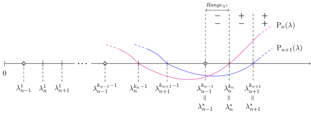
Figure 2: Real positive roots of $\mathrm{P}_{n+1}(\lambda)$, $\mathrm{P}_{n}(\lambda)$, and $\mathrm{P}_{n-1}(\lambda)$. Each eigenvalue sequence $\lambda^{p}_{n+b}$ is ordered increasingly, but the relative ordering in which the sequences are merged in the figure is arbitrary, except $\lambda^{*}_{n-1},\lambda^{*}_{n}$ and $\lambda^{*}_{n+1}$. Note that in the range $Range_{\lambda^{*}}$ that are no roots of $\mathrm{P}_{n+b}(\lambda)$ for $b\in\{-1,0,1\}$.

Claim 4.19

$\lambda_{n}^{p_{0}},\lambda_{n+1}^{p_{1}}\notin Range_{\lambda^{*}}$ for every real $\lambda_{n}^{p_{0}},\lambda_{n+1}^{p_{1}}$, for $p_{0}<k_{n},p_{1}<k_{n+1}$.

Proof: Note that $Z(\mathcal{L}_{n-1})$ is the principal $(n-1)$ minor of both $Z(\mathcal{L}_{n})$ and $Z(\mathcal{L}_{n+1})$. By the separation theorem of Hall and Porsching, see Lemma. 2.3, we get that $\lambda_{n}^{p_{0}},\lambda_{n+1}^{p_{1}}\leq\lambda_{n-1}^{*}$ for every $p_{0}<k_{n}$ and $p_{1}<k_{n+1}$, concluding by Eq. (26) that $\lambda_{n}^{p_{0}},\lambda_{n+1}^{p_{1}}\notin Range_{\lambda^{*}}$.     

We proceed by showing that $\mathrm{P}_{n}(\lambda)$ and $\mathrm{P}_{n+1}(\lambda)$ have the same sign in $Range_{\lambda^{*}}$. See Fig. 2 for a schematic description of the system.

Claim 4.20

$\mathrm{sign}(\mathrm{P}_{n}(\lambda))=\mathrm{sign}(\mathrm{P}_{n+1}(\lambda))$ for every $\lambda\in Range_{\lambda^{*}}$.

Proof: Fix $b\in\{0,1\}$. By Claim 4.19, $\mathrm{P}_{n+b}$ has no roots in $Range_{\lambda^{*}}$, so $\mathrm{sign}(\mathrm{P}_{n+b}(\lambda_{1}))=\mathrm{sign}(\mathrm{P}_{n+b}(\lambda_{2}))$ for every $\lambda_{1},\lambda_{2}\in Range_{\lambda^{*}}$. Also note that by Thm. 2.4, $\mathrm{sign}(\mathrm{P}_{n+b}(\lambda_{1}))=\mathrm{sign}(\mathrm{P}_{n+b}(\lambda_{2}))$, for every $\lambda_{1},\lambda_{2}>\lambda_{n+b}^{*}$. We now make two crucial observations. First, as $\mathrm{P}_{n}(\lambda)$ and $\mathrm{P}_{n+1}(\lambda)$ correspond to a characteristic polynomial of an $n\times n$ matrix, they have the same leading coefficient (any characteristic polynomial is monic, i.e., with leading coefficient 1 and degree $n$) and therefore $\mathrm{sign}(\mathrm{P}_{n}(\lambda))=\mathrm{sign}(\mathrm{P}_{n+1}(\lambda))$ for $\lambda>\lambda_{n+1}^{*}$ (recall that we assume that $\lambda_{n+1}^{*}\geq\lambda_{n}^{*}$). Second, due to the PF Theorem, the maximal roots of $\mathrm{P}_{n}(\lambda)$ and $\mathrm{P}_{n+1}(\lambda)$ are of multiplicity one and therefore the polynomial $\mathrm{P}_{n}(\lambda)$ (resp., $\mathrm{P}_{n+1}(\lambda)$) necessarily changes its sign when $\lambda$ passes through its maximal real positive root $\lambda_{n}^{*}$ (respectively, $\lambda_{n+1}^{*}$). Using these two observations, we now prove the claim via contradiction. Assume, toward contradiction, that $\mathrm{sign}(\mathrm{P}_{n}(\lambda))\neq\mathrm{sign}(\mathrm{P}_{n+1}(\lambda))$ for some $\lambda\in Range_{\lambda^{*}}$. Then $\mathrm{sign}(\mathrm{P}_{n}(\lambda_{1}))\neq\mathrm{sign}(\mathrm{P}_{n}(\lambda_{2}))$ for $\lambda_{1}>\lambda_{n}^{*}$ and $\lambda_{2}\in Range_{\lambda^{*}}$ also $\mathrm{sign}(\mathrm{P}_{n+1}(\lambda_{1}))\neq\mathrm{sign}(\mathrm{P}_{n+1}(\lambda_{2}))$ for $\lambda_{1}>\lambda_{n+1}^{*}$ and $\lambda_{2}\in Range_{\lambda^{*}}$. (This holds since when encountering a root of multiplicity one, the sign necessarily flips). In particular, this implies that $\mathrm{sign}(\mathrm{P}_{n}(\lambda))\neq\mathrm{sign}(\mathrm{P}_{n+1}(\lambda))$ for every $\lambda\geq\lambda_{n+1}^{*}$, in contradiction to the fact that $\mathrm{sign}(\mathrm{P}_{n}(\lambda))=\mathrm{sign}(\mathrm{P}_{n+1}(\lambda))$ for every $\lambda>\lambda_{n+1}^{*}$. The claim follows.     

We now complete the proof of Lemma 4.15.

Proof: By Eqs. (25) and (26), $\mathrm{P}_{n-1}(\lambda)\neq 0$ for every $\lambda\in Range_{\lambda^{*}}$. We can safely apply Claim 4.20 to Lemma 4.18 and and get that $\mathrm{sign}(X^{*}(n))\neq\mathrm{sign}(X^{*}(n+1))$. Since $X^{*}(n),X^{*}(n+1)$ and $g(n,n),g(n,n+1)$ are nonnegative, it follows that $X^{*}(n)=0$ and $X^{*}(n+1)=0$. In contradiction to Lemma 4.3. We conclude that $\beta^{*}=\beta^{*}_{n}$.     

We complete the geometric characterization of the generalized PF Theorem by noting the following.

Lemma 4.21

Every vertex $\overline{X}\in V(\mathcal{P}(\beta^{*}))$ is a $\boldsymbol{0^{*}}$ solution.

Proof: By Lemma 4.11, it is sufficient to show that there exists no $\overline{X}\in V(\mathcal{P}(\beta^{*}))$ that is weak, namely, which is a $\boldsymbol{{}_{w}0^{*}}$ solution but not a $\boldsymbol{0^{*}}$ solution. Assume, towards contradiction, that $\overline{X}\in V(\mathcal{P}(\beta^{*}))$ and that both $X(n)>0$ and $X(n+1)>0$. From now on, we replace $\overline{X}\in\mathbb{R}^{m}$ by its truncated sub-vector in $\mathbb{R}^{n+1}$, i.e., we discard the $m-n-1$ zero entries in $\overline{X}$.

Let $\mathcal{L}_{n-1},\mathcal{L}_{n}$ and $\mathcal{L}_{n+1}$ be defined as in Eq. (23). Recalling the notation of Sec. 2 where for matrix $A$, we denote $A_{-(i,j)}$ by the matrix that results from $A$ by removing the $i$-th row and the $j$-th column, define

$$a_{i}=(-1)^{n-i}\cdot\frac{\det\left(W^{2}(\mathcal{L}_{n},\beta^{*})_{-(n,i)}\right)}{\det\left(W^{2}(\mathcal{L}_{n-1},\beta^{*})\right)}$$

and

$$b_{i}=(-1)^{n-i}\cdot\frac{\det\left(W^{2}(\mathcal{L}_{n+1},\beta^{*})_{-(n,i)}\right)}{\det\left(W^{2}(\mathcal{L}_{n-1},\beta^{*})\right)}$$

for $i\in\{1,\ldots,n\}$. By Eq. (3), Claim 2.2(a) and the proof of Lemma 4.18, every optimal solution, and in particular every $\overline{X}\in V(\mathcal{P}(\beta^{*}))$, satisfies

$$X(i)=a_{i}\cdot X(n)+b_{i}\cdot X(n+1)$$ (27)

for $i\in\{1,\ldots,n-1\}$. This implies that our weak solution $\overline{X}$ is given by

$$\overline{X}~{}=~{}X(n)\cdot[a_{1},\ldots,a_{n-1},1,0]^{T}+X(n+1)\cdot[b_{1},\ldots,b_{n-1},0,1]^{T}.$$

Let

$$c_{n}~{}=~{}X(n)\cdot\left(1+\sum_{i=1}^{n-1}a_{i}\right)$$

and

$$c_{n+1}=X(n+1)\cdot\left(1+\sum_{i=1}^{n-1}b_{i}\right),$$

where the feasibility of $\overline{X}$ implies $c_{n}+c_{n+1}=1$. Next, consider Lemma 4.18. Since $\overline{X}$ is optimal, with both $X(n)>0$ and $X(n+1)>0$, it follows that $\det\left(W^{2}(\mathcal{L}_{n},\beta^{*})\right)=\det\left(W^{2}(\mathcal{L}_{n+1},\beta^{*})\right)=0$. This means that when constructing an optimal solution $\overline{Y}$, one has complete freedom to select any $Y(n),Y(n+1)\geq 0$ and the rest of the coordinates are determined by Eq. (27). In particular, setting $Y(n)=X(n)/c_{n}$ and $Y(n+1)=X(n+1)/c_{n+1}$ yields the following two optimal solutions: $\overline{Y}_{1}=X(n)/c_{n}\cdot[a_{1},\ldots,a_{n-1},1,0]^{T}$ and $\overline{Y}_{2}=X(n+1)/c_{n+1}\cdot[b_{1},\ldots,b_{n-1},0,1]^{T}$. Note that $\overline{X}$ can be described as a convex combination of $\overline{Y}_{1}$ and $\overline{Y}_{2}$, i.e., $\overline{X}=c_{n}\cdot\overline{Y}_{1}+c_{n+1}\cdot\overline{Y}_{2}$ (recall that $c_{n}+c_{n+1}=1$). This is in contradiction to the fact that $\overline{X}$ is a vertex of a polytope. The lemma follows.     

Lemma 4.22

There exists a selection $F^{*}\in\mathcal{F}$ such that $\mathit{r}(\mathcal{L}(F^{*}))=1/\beta^{*}$.

Proof: Recall that our $\boldsymbol{0^{*}}$ solution, $\overline{X}^{*}$, is a solution for the weak subsystem $\mathcal{L}^{W}$, and therefore $\overline{X}^{*}\in\mathbb{R}^{n+1}$. In addition, $|NZ(\overline{X}^{*})|=n$ and due to Lemma 4.3, $|NZ(\overline{X}^{*})\cap\mathcal{S}_{i}|=1$ for every $\mathit{v}_{i}$, or in other words, $\mathbb{S}^{\prime}=NZ(\overline{X}^{*})$ is a complete selection for $\mathcal{V}$ such that $|\mathbb{S}^{\prime}|=n$. Taking $F^{*}=F(\mathbb{S}^{\prime})$ yields the desired claim. The lemma follows.     

Note that Eq. (27) illustrates the additional degrees of freedom at the optimum point of Program (5). Specifically, to obtain an optimum solution for $\beta^{*}$, one has the freedom to set $X_{n}\geq 0$ and $X_{n+1}\geq 0$ (as long as at least one of them is positive) and the rest of the coordinates are determined accordingly.

We are now ready to complete the proof of Thm. 3.9.

Proof: [Thm. 3.9] Let $F^{*}$ be the selection such that $\mathit{r}(\mathcal{L})=\mathit{r}(\mathcal{L}(F^{*}))$. Note that by the irreducibility of $\mathcal{L}$, the square system $\mathcal{L}(F^{*})$ is irreducible as well and therefore the PF Theorem  for irreducible matrices can be applied. In particular, by Thm. 2.4, it follows that $\mathit{r}(\mathcal{L}(F^{*}))\in\mathbb{R}_{>0}$ and that $\mathbf{\overline{P}}(\mathcal{L}(F^{*}))>0$. Therefore, by Eq. (11) and (12), Claims (Q1)-(Q3) of Thm. 3.9 follow.

We now turn to claim (Q4) of the theorem. Note that for a symmetric system, in which $g(i,j_{1})=g(i,j_{2})$ for every $\mathcal{A}_{j_{1}},\mathcal{A}_{j_{2}}\in\mathcal{S}_{k}$ and every $k,i\in[1,n]$, the system is invariant to the selection matrix and therefore $\mathit{r}(\mathcal{L}(F_{1}))=\mathit{r}(\mathcal{L}(F_{2}))$ for every $F_{1},F_{2}\in\mathcal{F}$.

Finally, it remains to consider claim (Q5) of the theorem. Note that the optimization problem specified by Program (5) is an alternative formulation to the generalized Collatz-Wielandt formula given in (Q5). We now show that $\mathit{r}(\mathcal{L})$ (respectively, $\mathbf{\overline{P}}(\mathcal{L})$) is the optimum value (resp., point) of Program (5). By Lemma 4.22, there exists an optimal point $\overline{X}^{*}$ for Program (5) which is a $\boldsymbol{0^{*}}$ solution. Note that a $\boldsymbol{0^{*}}$ solution corresponds to a unique hidden square system, given by $\mathcal{L}^{*}=\mathcal{L}(NZ(\overline{X}^{*}))$ ($\mathcal{L}^{*}$ is square since $|NZ(\overline{X}^{*})|=n$). Therefore, by Thm. 2.6 and Lemma 4.22, we get that

$$\mathit{r}(\mathcal{L}^{*})~{}=~{}1/\beta^{*}(\mathcal{L}^{*})~{}=~{}1/\beta^{*}(\mathcal{L}).$$ (28)

Next, by Observation 3.4(b), we have that $\mathit{r}(\mathcal{L}(F))\geq\mathit{r}(\mathcal{L})$. It therefore follows that

$$\mathit{r}(\mathcal{L}^{*})~{}=~{}\min_{F\in\mathcal{F}}\mathit{r}(\mathcal{L}(F)).$$ (29)

Combining Eq. (28), (29) and (11), we get that the PF eigenvalue of the system $\mathcal{L}$ satisfies $\mathit{r}(\mathcal{L})=1/\beta^{*}(\mathcal{L})$ as required. Finally, note that by Thm. 2.6, $\mathbf{\overline{P}}(\mathcal{L}^{*})$ is the optimal point for Program (5) with the square system $\mathcal{L}^{*}$. By Eq. (12), $\mathbf{\overline{P}}(\mathcal{L})$ is an extension of $\mathbf{\overline{P}}(\mathcal{L}^{*})$ with zeros (i.e., a $\boldsymbol{0^{*}}$ solution). It can easily be checked that $\mathbf{\overline{P}}(\mathcal{L})$ is a feasible solution for the original system $\mathcal{L}$ with $\beta=\beta^{*}(\mathcal{L}^{*})=\beta^{*}(\mathcal{L})$, hence it is optimal. Note that by Lemma 4.12, it indeed follows that $\mathcal{M}^{-}\cdot\mathbf{\overline{P}}(\mathcal{L})=1/\beta^{*}(\mathcal{L})\cdot\mathcal{M}^{+}\cdot\mathbf{\overline{P}}(\mathcal{L})$, for every optimal solution $\overline{X}^{*}$. Theorem 3.9 follows.     

5 Computing the generalized PF vector

In this section we present a polynomial time algorithm for computing the generalized Perron eigenvector $\mathbf{\overline{P}}(\mathcal{L})$ of an irreducible system $\mathcal{L}$.

The method.

By Property (Q5) of Thm. 3.9, computing $\mathbf{\overline{P}}(\mathcal{L})$ is equivalent to finding a $\boldsymbol{0^{*}}$ solution for Program (5) with $\beta=\beta^{*}(\mathcal{L})$. For ease of analysis, we assume throughout that the gains are integral, i.e., $g(i,j)\in\mathbb{Z}^{+}$, for every $i\in\{1,\ldots,n\}$ and $j\in\{1,\ldots,m\}$. If this does not hold, then the gains can be rounded or scaled to achieve this. Let

$$\mathcal{G}_{max}(\mathcal{L})~{}=~{}\max_{i\in\{1,\ldots,n\},j\in\{1,\ldots,m\}}\left\{|g(i,j)|\right\},$$ (30)

and define $\mbox{T}_{LP}$ as the running time of an LP solver such as the interior point algorithm [6] for Program (15). Recall that we look for an exact optimal solution for a non-convex optimization problem (see Program (5)). Using the convex relaxation of Program (15), a binary search can be applied for finding an approximate solution up to a predefined accuracy. The main challenge is then to find (a) an optimal solution (and not an approximate one), and (b) among all the optimal solutions, to find one that is a $\boldsymbol{0^{*}}$ solution. Let $F_{1},F_{2}\in\mathcal{F}$ be two selection matrices for $\mathcal{L}$. By Thm. 3.9, there exists a selection matrix $F^{*}$ such that $\mathit{r}(\mathcal{L})=\mathit{r}(\mathcal{L}(F^{*}))$ and $\mathbf{\overline{P}}(\mathcal{L})$ is a $\boldsymbol{0^{*}}$ solution corresponding to $\mathbf{\overline{P}}(\mathcal{L}(F^{*}))$ (in addition $\beta^{*}=1/\mathit{r}(\mathcal{L}(F^{*}))$). Our goal then is to find a selection matrix $F^{*}\in\mathcal{F}$ where $|\mathcal{F}|$ might be exponentially large.

Theorem 5.1

Let $\mathcal{L}$ be an irreducible system. Then $\mathbf{\overline{P}}(\mathcal{L})$ can be computed in time $O(n^{3}\cdot\mbox{T}_{LP}\cdot\left(\log\left(n\cdot\mathcal{G}_{max}\right)+n\right))$.

Let

$$\Delta_{\beta}~{}=~{}(n\mathcal{G}_{max})^{-8n^{3}}.$$ (31)

The key observation in this context is the following “minimum gap” observation.

Lemma 5.2

Consider a selection matrix $F\in\mathcal{F}$. If $\beta^{*}(\mathcal{L})-1/\mathit{r}(\mathcal{L}(F))\leq\Delta_{\beta}$, then $\beta^{*}(\mathcal{L})=1/\mathit{r}(\mathcal{L}(F))$.

By performing a polynomial number of steps of binary search for the optimal $\beta^{*}(\mathcal{L})$, one can converge to a value $\beta^{-}$ that is at most $\Delta_{\beta}$ far from $\beta^{*}(\mathcal{L})$, i.e., $\beta^{*}(\mathcal{L})-\beta^{-}<\Delta_{\beta}$. Let $Range_{\beta^{*}}=[\beta^{-},\beta^{*}]$. Then by Lemma 4.22, we are guaranteed that $\mathit{r}(\mathcal{L}(F))=1/\beta^{*}$ for any selection matrix $F\in\mathcal{F}$ such that $1/\mathit{r}(\mathcal{L}(F))\in Range_{\beta^{*}}$ (there could be many such matrices $F$, but in this case, they all correspond to systems with PF value $1/\beta^{*}$). To prove Lemma 5.2, we first establish a lower bound on the difference between any two different PF eigenvalues of any two irreducible square systems, i.e., we show that the PF roots $\mathit{r}(\mathcal{L}^{s}_{1})$ and $\mathit{r}(\mathcal{L}^{s}_{2})$ of any two irreducible square systems $\mathcal{L}^{s}_{1},\mathcal{L}^{s}_{2}\in\mathfrak{L}^{S}$ cannot be too close if they are different. Recall that for an irreducible square system $\mathcal{L}^{s}$, $Z(\mathcal{L}^{s})=(\mathcal{M}^{+})^{-1}\cdot\mathcal{M}^{-}$, where $\mathcal{M}^{+}$ can be considered to be diagonal with a strictly positive diagonal. We begin the analysis by scaling the entries of $Z(\mathcal{L}^{s})$ to obtain an integer-valued matrix $Z^{\mathrm{int}}$. The scaling is needed in order to employ a well-known bound due to Bugeaud and Mignotte [7] on the minimal distance between the roots of integer polynomials (Lemma 5.3). The guaranteed distance on $\mathit{r}(\mathcal{L}^{s}_{1})$ and $\mathit{r}(\mathcal{L}^{s}_{2})$ is later translated into a minimal bound on distance for their reciprocals $1/\mathit{r}(\mathcal{L}^{s}_{1})$ and $1/\mathit{r}(\mathcal{L}^{s}_{2})$, which correspond to $\beta$ values of Program (5), i.e., optimal $\beta$ values of two different irreducible square systems for Program (5). Specifically, we show that for any given sufficiently small range of $\beta$ values, $Range_{\beta}=[\beta_{1},\beta_{2}]$ such that $|\beta_{1}-\beta_{2}|\leq\Delta_{\beta}$, there cannot be two selection matrices $F_{1},F_{2}\in\mathcal{F}$ such that $\mathit{r}(\mathcal{L}(F_{1}))\neq\mathit{r}(\mathcal{L}(F_{2}))$ and yet both $1/\mathit{r}(\mathcal{L}(F_{1})),1/\mathit{r}(\mathcal{L}(F_{2}))\in Range_{\beta}$.

The naïve height of an integer polynomial $P$, denoted $H(P)$, is the maximum of the absolute values of its coefficients.

Lemma 5.3 (Bugeaud and Mignotte [7])

Let $P(X)$ and $Q(X)$ be nonconstant integer polynomials of degree $n$ and $m$, respectively. Denote by $r_{P}$ and $r_{Q}$ a zero of $P(X)$ and $Q(X)$, respectively. Assuming that $P(r_{Q})\neq 0$, we have

$$|\ r_{P}-r_{Q}|\ \geq 2^{1-n}(n+1)^{\frac{1}{2}-m}(m+1)^{-\frac{n}{2}}H(P)^{-m}H(Q)^{-n}.$$

We first show the following.

Lemma 5.4

$|\mathit{r}(\mathcal{L}^{s}_{1})-\mathit{r}(\mathcal{L}^{s}_{2})|\geq(n\mathcal{G}_{max})^{-6n^{3}}$ for every $\mathcal{L}^{s}_{1},\mathcal{L}^{s}_{2}\in\mathfrak{L}^{S}$.

Proof: Recall that for an irreducible square system $\mathcal{L}^{s}$, $Z(\mathcal{L}^{s})=(\mathcal{M}^{+})^{-1}\cdot\mathcal{M}^{-}$, where $\mathcal{M}^{+}$ can be considered to be diagonal with strictly positive diagonal. Therefore, $Z(\mathcal{L}^{s})_{i,j}=|g(i,j)|/g(i,i)$ where $g(i,i)$ corresponds to the gain of the unique supporter of $\mathit{v}_{i}$.

For ease of notation, let $Z_{1}=Z(\mathcal{L}^{s}_{1})$, $Z_{2}=Z(\mathcal{L}^{s}_{2})$, $r_{1}=\mathit{r}(\mathcal{L}^{s}_{1})$ and $r_{2}=\mathit{r}(\mathcal{L}^{s}_{2})$. Let $i_{1}$ (resp., $i_{2}$) be the index of the unique supporter of entity $\mathit{v}_{i}$ in the square system $\mathcal{L}^{s}_{1}$ (resp., $\mathcal{L}^{s}_{2}$).

To employ Lemma 5.3, we first scale $Z_{1}$ and $Z_{2}$ to obtain two integer-valued matrices $Z^{\mathrm{int}}_{1}$ and $Z^{\mathrm{int}}_{2}$. The new matrix $Z_{b}^{\mathrm{int}}$, for $b\in\{1,2\}$, is constructed by multiplying each entry of $Z_{b}$ by the common denominator of its entries, i.e., $Z_{b}^{\mathrm{int}}(i,j)=Z_{b}(i,j)\cdot\prod_{i}\left(|g(i,i_{1})|\cdot|g(i,i_{2})|\right)$. Thus all entries of $Z_{b}^{\mathrm{int}}$ are integers and bounded by $\mathcal{G}_{max}^{2n}$ (since $|g(i,j)|\leq\mathcal{G}_{max}$). Let $P_{1}(x)=\mathrm{P}(Z^{\mathrm{int}}_{1},x)$ and $P_{2}(x)=\mathrm{P}(Z^{\mathrm{int}}_{2},x)$ be the characteristic polynomials of the matrices $Z^{\mathrm{int}}_{1}$ and $Z^{\mathrm{int}}_{2}$ respectively, see Eq. (3). Note that $P_{1}(x)$ and $P_{2}(x)$ are integer polynomials of degree $n$, and $H(P_{1}),H(P_{2})\leq\mathcal{G}_{max}^{2n^{2}}$ (since $|\det(Z)|\leq(\mathcal{G}_{max}^{2n})^{n}$). Let $r_{1}^{\mathrm{int}}$ and $r_{2}^{\mathrm{int}}$ correspond to the PF eigenvalues of $Z_{1}^{\mathrm{int}}$ and $Z_{2}^{\mathrm{int}}$ respectively. Lemma 5.3 yields

$$|r_{1}^{\mathrm{int}}-r_{2}^{\mathrm{int}}| \geq 2^{1-n}(n+1)^{\frac{1}{2}-n}(n+1)^{-\tfrac{n}{2}}(\mathcal{G}_{max}^{2n^{2}})^{-n}(\mathcal{G}_{max}^{2n^{2}})^{-n}=2^{1-n}(n+1)^{\frac{1-3n}{2}}\mathcal{G}_{max}^{-4n^{3}}.$$

Finally, by definition of $Z^{\mathrm{int}}_{1}$ and $Z^{\mathrm{int}}_{2}$,

$$|r_{1}^{\mathrm{int}}-r_{2}^{\mathrm{int}}|~{}=~{}|r_{1}-r_{2}|\prod_{i}\left(|g(i,i_{1})|\cdot|g(i,i_{2})|\right),$$

and thus

$$|r_{1}-r_{2}| \geq \frac{2^{1-n}(n+1)^{\frac{1-3n}{2}}\mathcal{G}_{max}^{-4n^{3}}}{\prod_{i}\left(|g(i,i_{1})|\cdot|g(i,i_{2})|\right)}~{}\geq~{}\frac{2^{1-n}(n+1)^{\frac{1-3n}{2}}\mathcal{G}_{max}^{-4n^{3}}}{\mathcal{G}_{max}^{2n}}\geq(n\mathcal{G}_{max})^{-6n^{3}}.$$

   

We now turn to translate the distance between $r_{1}$ and $r_{2}$ into a distance between $1/r_{1}$ and $1/r_{2}$ (corresponding to the optimal $\beta$ values of Program (5) with $\mathcal{L}^{s}_{1}$ and $\mathcal{L}^{s}_{2}$, respectively). The next auxiliary claim gives a bound for $\lambda\in EigVal(A)$ as a function of $\mathcal{G}_{max}$.

Lemma 5.5

Let $\lambda$ be an eigenvalue of an $n\times n$ matrix $Z$ such that $|Z(i,j)|\leq\mathcal{G}_{max}$. Then $|\lambda|\leq n\mathcal{G}_{max}$.

Proof: Let $\overline{X}$ be the eigenvector of $Z$ and assume that $||\overline{X}||_{2}=1$. Since $\overline{X}^{T}\cdot Z\cdot\overline{X}=\lambda\overline{X}^{T}\cdot\overline{X}=\lambda$, we have:

$$|\lambda| = |\overline{X}^{T}Z\overline{X}|~{}=~{}|\sum_{i}\sum_{j}X(i)Z(i,j)X(j)|~{}\leq~{}\mathcal{G}_{max}\cdot|\sum_{i}\sum_{j}X(i)\cdot X(j)|$$

$$= \mathcal{G}_{max}\cdot|\sum_{i}X(i)|\cdot|\sum_{j}X(j)|~{}=~{}\mathcal{G}_{max}\cdot\|\overline{X}\|_{1}^{2}~{}\leq~{}\mathcal{G}_{max}\cdot(\sqrt{n}\|\overline{X}\|_{2})^{2}~{}=~{}n\mathcal{G}_{max}~{}.$$

   

We now turn to prove Lemma 5.2.

Proof: [of Lemma 5.2]
By Lemma 5.4 and 5.5,

$$\left|\frac{1}{r_{2}}-\frac{1}{r_{1}}\right|=\left|\frac{r_{1}-r_{2}}{r_{1}r_{2}}\right|\geq\frac{\left|r_{1}-r_{2}\right|}{(n\mathcal{G}_{max})^{2}}\geq(n\mathcal{G}_{max})^{-8n^{3}}.$$

So far, we proved that if $\mathit{r}(\mathcal{L}(F_{1}))\not=\mathit{r}(\mathcal{L}(F_{2}))$, then $|1/\mathit{r}(\mathcal{L}(F_{1}))-1/\mathit{r}(\mathcal{L}(F_{2}))|\geq\Delta_{\beta}$, for every $F_{1},F_{2}\in\mathcal{F}$. By Thm. 3.9, there exists a selection $F^{*}\in\mathcal{F}$ such that $\mathit{r}(\mathcal{L}(F^{*}))=1/\beta^{*}(\mathcal{L})$. Assume, toward contradiction, that there exists some $F^{{}^{\prime}}\in\mathcal{F}$ such that $\mathit{r}(\mathcal{L}(F^{{}^{\prime}}))\neq 1/\beta^{*}(\mathcal{L})$ but $|\beta^{*}(\mathcal{L})-1/\mathit{r}(\mathcal{L}(F^{{}^{\prime}}))|\leq\Delta_{\beta}$. Let $r_{1}=\mathit{r}(\mathcal{L}(F^{*}))$ and $r_{2}=\mathit{r}(\mathcal{L}(F^{{}^{\prime}}))$. In this case, we get that $|1/r_{1}-1/r_{2}|\leq\Delta_{\beta}$, contradiction. Lemma 5.2 follows.     

Algorithm description.

We now describe Algorithm $\tt Compute\mathbf{\overline{P}}(\mathcal{L})$ for $\mathbf{\overline{P}}(\mathcal{L})$ computation. Consider some partial selection $\mathbb{S}^{\prime}\subseteq\mathcal{A}$ for $V^{\prime}\subseteq\mathcal{V}$. For ease of notation, let $\mathcal{L}(\mathbb{S}^{\prime})=\langle\mathcal{M}^{-}(\mathbb{S}^{\prime}),\mathcal{M}^{+}(\mathbb{S}^{\prime})\rangle$, where $\mathcal{M}^{-}(\mathbb{S}^{\prime})=\mathcal{M}^{-}\cdot F(\mathbb{S}^{\prime})$ and $\mathcal{M}^{+}(\mathbb{S}^{\prime})=\mathcal{M}^{+}\cdot F(\mathbb{S}^{\prime})$. Consider the Program

maximize $$~{}\beta\text{~{}subject to:~{}}$$ (32)

$$\displaystyle\mathcal{M}^{-}(\mathbb{S}^{\prime})\cdot\overline{X}\leq 1/\beta\cdot\mathcal{M}^{+}(\mathbb{S}^{\prime})\cdot\overline{X},$$

$$\displaystyle\overline{X}\geq\overline{0},$$

$$\displaystyle||\overline{X}||_{1}~{}=~{}1~{}.$$

Note that if $\mathbb{S}^{\prime}=\emptyset$, then Program (32) is equivalent to Program (5), i.e., $\mathcal{L}(\mathbb{S}^{\prime})=\mathcal{L}$. Define

$$f(\beta,\mathcal{L}(\mathbb{S}^{\prime}))=\left\{\begin{array}[]{ll}1,&\mbox{if there exists an~{}}\overline{X}\mbox{ such that }||\overline{X}||_{1}~{}=~{}1,~{}\overline{X}\geq\overline{0},\mbox{ and }\\ &\displaystyle\mathcal{M}^{-}(\mathbb{S}^{\prime})\cdot\overline{X}\leq 1/\beta\cdot\mathcal{M}^{+}(\mathbb{S}^{\prime})\cdot\overline{X},\\ 0,&\hbox{otherwise}.\end{array}\right.$$

Note that $f(\beta,\mathcal{L}(\mathbb{S}^{\prime}))=1$ iff $\mathcal{L}(\mathbb{S}^{\prime})$ is feasible for $\beta$ and that $f$ can be computed in polynomial time using the interior point method.

Algorithm $\tt Compute\mathbf{\overline{P}}(\mathcal{L})$ is composed of two main phases. In the first phase it finds, using binary search, an estimate $\beta^{-}$ such that $\beta^{*}(\mathcal{L})-\beta^{-}\leq\Delta_{\beta}$. In the second phase, it finds a hidden square system $\mathcal{L}(F^{*})$, $F^{*}\in\mathcal{F}$, corresponding to a complete selection vector $\mathbb{S}_{n}$ of size $n$ for $\mathcal{V}$. By Lemma 5.2, it follows that $\mathit{r}(\mathcal{L}(F^{*}))=1/\beta^{*}(\mathcal{L})$.

We now describe the construction of $\mathbb{S}_{n}$ in more detail. The second phase consists of $n$ iterations. Iteration $t$ obtains a partial selection $\mathbb{S}_{t}$ for $\mathit{v}_{1},\ldots,\mathit{v}_{t}$ such that $f(\beta^{-},\mathcal{L}(\mathbb{S}_{t}))=1$. The final step achieves the desired $\mathbb{S}_{n}$, where $\mathcal{L}(\mathbb{S}_{n})\in\mathfrak{L}^{S}$ and $f(\beta^{-},\mathcal{L}(\mathbb{S}_{n}))=1$ (therefore also $f(\beta^{-},\mathcal{L}(F(\mathbb{S}_{n})))=1$). Initially, $\mathbb{S}_{0}$ is empty. The $t$’th iteration sets $\mathbb{S}_{t}=\mathbb{S}_{t-1}\cup\{\mathcal{A}_{j}\}$ for some supporter $\mathcal{A}_{j}\in\mathcal{S}_{t}$ such that $f(\beta^{-},\mathcal{L}(\mathbb{S}_{t-1}\cup\{\mathcal{A}_{j}\}))=1$. We later show (in proof of Thm. 5.1) that such a supporter $\mathcal{A}_{j}$ exists.

Finally, we use $\mathbf{\overline{P}}(\mathcal{L}(\mathbb{S}_{n}))$ to construct the Perron vector $\mathbf{\overline{P}}(\mathcal{L})$. This vector contains zeros for the $m-n$ non-selected affectors, and the values of the $n$ selected affectors are as in $\mathbf{\overline{P}}(\mathcal{L}(\mathbb{S}_{n}))$.

The pseudocode is presented formally next.

Algorithm $\tt Compute\mathbf{\overline{P}}(\mathcal{L})$ /* Binary search phase: finding $\beta^{-}$ such that $\beta^{*}-\beta^{-}<\Delta_{\beta}$ */ 1. $\beta\leftarrow 1$; 2. While $f(\beta,\mathcal{L})=1$ do:
         $\beta\leftarrow 2\beta$; 3. If $\beta>1$, then $\beta^{-}\leftarrow\beta/2$, else $\beta^{-}\leftarrow 0$; 4. $\beta^{+}\leftarrow\beta$; 5. While $\beta^{+}-\beta^{-}\geq\Delta_{\beta}$ do:     /* from now on $\beta^{-}\leq\beta^{*}<\beta^{+}$ */ (a) $\beta\leftarrow\left(\beta^{-}+\beta^{+}\right)/{2}$; (b) If $f(\beta,\mathcal{L})=1$, then $\beta^{-}\leftarrow\beta$, else $\beta^{+}\leftarrow\beta$; /* Affector elimination phase: Finding a $\boldsymbol{0^{*}}$ solution */ 6. $\mathbb{S}_{0}\leftarrow\emptyset$; 7. For $t=1$ to $n$ do: (a) Select some supporter $\mathcal{A}_{j}\in\mathcal{S}_{t}$ such that $f(\beta^{-},\mathcal{L}(\mathbb{S}_{t}\cup\{\mathcal{A}_{j}\}))=1$; (b) Set $\mathbb{S}_{t+1}\leftarrow\mathbb{S}_{t}\cup\{\mathcal{A}_{j}\}$; /* $|\mathbb{S}_{n}|=n$ and $\mathcal{L}(\mathbb{S}_{n})\in\mathfrak{L}^{S}$  */ 8. Set Perron value $\beta^{*}=1/r(\mathcal{L}(\mathbb{S}_{n}))$; 9. Set $\overline{X}^{*}\leftarrow\mathbf{\overline{P}}(\mathcal{L}(\mathbb{S}_{n}))$; 10. Set $X^{**}(\mathcal{A}_{k})\leftarrow\begin{cases}X^{*}(\mathcal{A}_{k}),&\mathcal{A}_{k}\in\mathbb{S}_{n},\\ 0,&\text{otherwise;}\end{cases}$ 11. Let $\mathbf{\overline{P}}(\mathcal{L})\leftarrow\overline{X}^{**}$;

To establish Theorem 5.1, we prove the correctness of Algorithm $\tt Compute\mathbf{\overline{P}}(\mathcal{L})$ and bound its runtime. We begin with two auxiliary claims.

Claim 5.6

$\beta^{*}(\mathcal{L})\leq\mathcal{G}_{max}$.

Proof: Let $\overline{X}^{*}=\mathbf{\overline{P}}(\mathcal{L})$ and let $\mathbb{S}^{*}=NZ(\overline{X}^{*})$. Then by claims (Q3) and (Q5) of Thm. 3.9 we have that $|\mathbb{S}^{*}|=n$. Define $F^{*}=F(\mathbb{S}^{*})$. Since $\mathbb{S}^{*}$ is a complete selection vector (see Claim 4.3), we have that $F^{*}\in\mathcal{F}$. Let $\mathcal{A}_{\gamma(i)}$ be the supporter of entity $\mathit{v}_{i}$ in $\mathbb{S}^{*}$, for every $i\in\{1,\ldots,n\}$.

Let $D=\mathcal{CG}_{\mathcal{L}(F^{*})}$. Since $\mathcal{L}$ is irreducible, it follows by Obs. 3.6 that $D$ is strongly connected. Let $C=(\mathit{v}_{i_{1}},\ldots,\mathit{v}_{i_{k}})$ be a directed cycle in $D$, i.e., $(\mathit{v}_{i_{j}},\mathit{v}_{i_{j+1}})\in E(D)$ for every $j\in\{1,\ldots,k\}$ and $(\mathit{v}_{i_{k}},\mathit{v}_{i_{1}})\in E(D)$. For ease of notation, let $\mathit{v}_{i_{k}}=\mathit{v}_{i_{-1}}$. Since $D$ is strongly connected, such a cycle $C$ exists. By the optimality of $\overline{X}^{*}$ we have that

$$\beta^{*}(\mathcal{L})\cdot T^{-}(\overline{X}^{*},\mathcal{L})_{i}~{}=~{}T^{+}(\overline{X}^{*},\mathcal{L})_{i}$$

for every $\mathit{v}_{i}$. Note that by definition $|g(\mathit{v}_{i_{j}},\mathcal{A}_{\gamma(i_{j-1})})|\cdot X^{*}(\mathcal{A}_{\gamma(i_{j-1})})\leq T^{-}(\overline{X}^{*},\mathcal{L})_{i_{j}}$ for every $j\in\{1,\ldots,k\}$, and by the graph definition, $\mathcal{A}_{\gamma(i_{j-1})}\in\mathcal{R}_{i_{j}}$ or $g(\mathit{v}_{i_{j}},\mathcal{A}_{\gamma(i_{j-1})})<0$, for every $j\in\{1,\ldots,k\}$. Combining this with Fact 3.2, we get that

$$\beta^{*}(\mathcal{L})|g(\mathit{v}_{i_{j}},\mathcal{A}_{\gamma(i_{j-1})})|X^{*}(\mathcal{A}_{\gamma(i_{j-1})})~{}\leq~{}g(\mathcal{A}_{\gamma(i_{j})},\mathit{v}_{i_{j}})\cdot X^{*}(\mathcal{A}_{\gamma(i_{j})})$$

for every $j\in\{1,\ldots,k\}$, and therefore

$$\beta^{*}(\mathcal{L})~{}\leq~{}\min_{j\in\{1,\ldots,k\}}\left\{\frac{g(\mathcal{A}_{\gamma(i_{j})},\mathit{v}_{i_{j}})}{|g(\mathcal{A}_{\gamma(i_{j-1})},\mathit{v}_{i_{j}})|}\cdot\frac{X^{*}(\mathcal{A}_{\gamma(i_{j})})}{X^{*}(\mathcal{A}_{\gamma(i_{j-1})})}\right\}.$$

It is easy to verify that $\min_{j\in\{1,\ldots,k\}}\left\{\frac{X^{*}(\mathcal{A}_{\gamma(i_{j})})}{X^{*}(\mathcal{A}_{\gamma(i_{j-1})})}\right\}\leq 1$. Therefore, by Eq. (30) we get that $\beta^{*}(\mathcal{L})\leq\mathcal{G}_{max}$, as required.     

Lemma 5.7

Phase 1 of Alg. $\tt Compute\mathbf{\overline{P}}(\mathcal{L})$ finds $\beta^{-}$ such that $\beta^{*}(\mathcal{L})-\beta^{-}\leq\Delta_{\beta}$.

Proof: By Property (Q5) of Thm. 3.9, $\mathbf{\overline{P}}(\mathcal{L})$ is an optimal solution for Program (5) and $\mathit{r}(\mathcal{L})=1/\beta^{*}(\mathcal{L})$. Therefore $f(\beta,\mathcal{L})=1$ for every $\beta\in(0,\beta^{*}]$. Steps 3 and 5(b) in Alg. $\tt Compute\mathbf{\overline{P}}(\mathcal{L})$ yield $f(\beta^{-},\mathcal{L})=1$. Therefore $\beta^{-}\leq\beta^{*}(\mathcal{L})$. By the stopping criterion of step 5, it ends with $f(\beta^{+},\mathcal{L})=0$, $f(\beta^{-},\mathcal{L})=1$ and $\beta^{+}-\beta^{-}\leq\Delta_{\beta}$. The first 2 conditions imply that $\beta^{*}\in[\beta^{-},\beta^{+})$ as required. The claim follows.     

Let $Range_{\beta^{*}}=[\beta^{-},\beta^{+})$.

Lemma 5.8

By the end of phase 2, the selection $\mathbb{S}_{n}$ satisfies $\mathit{r}(\mathcal{L}(\mathbb{S}_{n}))=1/\beta^{*}(\mathcal{L})$.

Proof: Let $\mathbb{S}_{t}$ be the partial selection obtained at step $t$, $\mathcal{L}_{t}=\mathcal{L}(\mathbb{S}_{t})$ be the corresponding system for step $t$ and $\beta_{t}=\beta^{*}(\mathcal{L}_{t})$ the optimal solution of Program (5) for system $\mathcal{L}_{t}$. We claim that $\mathbb{S}_{t}$ satisfies the following properties for each $t\in\{0,\ldots,n\}$:

(C1) $\mathbb{S}_{t}$ is a partial selection vector of length $t$, such that $\mathbb{S}_{t}\sim\mathbb{S}_{t-1}$.

(C2) $\mathcal{L}(\mathbb{S}_{t})$ is feasible for $\beta^{-}$.

The proof is by induction. Beginning with $\mathbb{S}_{0}=\emptyset$, it is easy to see that (C1) and (C2) are satisfied (since $\mathcal{L}(\mathbb{S}_{0})=\mathcal{L}$). Next, assume that (C1) and (C2) hold for $\mathbb{S}_{i}$ for $i\leq t$ and consider $\mathbb{S}_{t+1}$. Let $V_{t}\subseteq\mathcal{V}$ be such that $\mathbb{S}_{t}$ is a partial selection for $V_{t}$ (i.e., $|V_{t}|=|\mathbb{S}_{t}|$, and $|\mathcal{S}_{i}(\mathcal{L})\cap\mathbb{S}_{t}|=1$ for every $\mathit{v}_{i}\in V_{t}$). Given that $\mathbb{S}_{t}$ is a selection for nodes $\mathit{v}_{1},\ldots,\mathit{v}_{t}$ that satisfies (C1) and (C2), we show that $\mathbb{S}_{t+1}$ satisfies (C1) and (C2) as well.

In particular, it is required to show that there exists at least one supporter of $\mathit{v}_{t+1}$, namely, $\mathcal{A}_{k}\in\mathcal{S}_{t+1}(\mathcal{L})$, such that $f(\beta^{-},\mathcal{L}(\mathbb{S}_{t}\cup\{\mathcal{A}_{k}\}))=1$. This will imply that step 7(a) of the algorithm always succeeds in expanding $\mathbb{S}_{t}$.

By Observation 3.7 and Property (C2) for step $t$, the system $\mathcal{L}(\mathbb{S}_{t})$ is irreducible with $\beta_{t}\geq\beta^{-}$. In addition, note that $\mathcal{F}(\mathcal{L}_{t})\subseteq\mathcal{F}(\mathcal{L})$ (as every square system of $\mathcal{L}_{t}$ is also a square system of $\mathcal{L}$). By Theorem 3.9, there exists a square system $\mathcal{L}_{t}(F^{*}_{t})$, $F^{*}_{t}\in F(\mathcal{L}_{t})$, such that $\mathit{r}(\mathcal{L}_{t}(F^{*}_{t}))=1/\beta_{t}$. In addition, $\mathbf{\overline{P}}(\mathcal{L}_{t}(F^{*}_{t}))$ is a feasible solution for Program (15) with the system $\mathcal{L}_{t}(F^{*}_{t})$ and $\beta=\beta_{t}$.

By Eq. (9), the square system $\mathcal{L}_{t}(F^{*}_{t})$ corresponds to a complete selection $\mathbb{S}^{**}$, where $|\mathbb{S}^{**}|=n$ and $\mathbb{S}_{t}\subseteq\mathbb{S}^{**}$, i.e., $\mathcal{L}_{t}(F^{*}_{t})=\mathcal{L}(\mathbb{S}^{**})$. Observe that by Property (Q5) of Thm. 3.9 for the system $\mathcal{L}_{t}$, there exists a $\boldsymbol{0^{*}}$ solution for Program (15) that achieves $\beta_{t}$. This $\boldsymbol{0^{*}}$ solution is constructed from $\mathbf{\overline{P}}(\mathcal{L}_{t}(\mathbb{S}^{**}))$, the PF eigenvector of $\mathcal{L}_{t}(\mathbb{S}^{**})$.

Let $\mathcal{A}_{k}\in\mathcal{S}_{t+1}(\mathcal{L}_{t})\cap\mathbb{S}^{**}$. Note that by the choice of $\mathbb{S}^{**}$, such an affector $\mathcal{A}_{k}$ exists. We now show that $\mathbb{S}_{t+1}=\mathbb{S}_{t}\cup\{\mathcal{A}_{k}\}$ satisfies Property (C2), thus establishing the existence of $\mathcal{A}_{k}\in\mathcal{S}_{t+1}(\mathcal{L}_{t})$ in step 7(a). We show this by constructing a feasible solution $X^{*}_{\beta^{-}}\in\mathbb{R}^{m(\mathbb{S}_{t+1})}$ for $\mathcal{L}_{t+1}$. By the definition of $\mathbb{S}^{**}$, $f(\beta^{-},\mathcal{L}(\mathbb{S}^{**}))=1$ and therefore there exists a feasible solution $\overline{X}^{t+1}_{\beta^{-}}\in\mathbb{R}^{n}$ for $\mathcal{L}(\mathbb{S}^{**})$. Since $\mathbb{S}_{t+1}\subseteq\mathbb{S}^{**}$, it is possible to extend $\overline{X}^{t+1}_{\beta^{-}}\in\mathbb{R}^{n}$ to a feasible solution $X^{*}_{\beta^{-}}$ for system $\mathcal{L}_{t+1}$, by setting $X^{*}_{\beta^{-}}(\mathcal{A}_{q})=X^{t+1}_{\beta^{-}}(\mathcal{A}_{q})$ for every $\mathcal{A}_{q}\in\mathbb{S}^{**}$ and $X^{*}_{\beta^{-}}(\mathcal{A}_{q})=0$ otherwise. It is easy to verify that this is indeed a feasible solution for $\beta^{-}$, concluding that $f(\beta^{-},\mathcal{L}_{t+1})=1$.

So far, we have shown that there exists an affector $\mathcal{A}_{k}\in\mathcal{S}_{t+1}(\mathcal{L}_{t})$ such that $f(\beta^{-},\mathcal{L}_{t+1})=1$. We now claim that for any $\mathcal{A}_{k}\in\mathcal{S}_{t+1}(\mathcal{L}_{t})$ such that $f(\beta^{-},\mathcal{L}_{t+1})=1$, Properties (C1) and (C2) are satisfied. This holds trivially, relying on the criterion for selecting $\mathcal{A}_{k}$, since $\mathcal{S}_{t+1}(\mathcal{L}_{t})\cap\mathbb{S}_{t}=\emptyset$.

After $n$ steps, we get that $\mathbb{S}_{n}$ is a complete selection, $F(\mathbb{S}_{n})\in\mathcal{F}(\mathcal{L}_{n-1})$, and therefore by Property (C1) for steps $t=1,\ldots,n$, it also holds that $F(\mathbb{S}_{n})\in\mathcal{F}(\mathcal{L})$. In addition, by Property (C2), $f(\beta^{-},\mathcal{L}_{n})=1$. Since $\mathcal{L}_{n}$ is equivalent to $\mathcal{L}(\mathbb{S}_{n})\in\mathfrak{L}^{S}$ (obtained by removing the $m-n$ columns corresponding to the affectors not selected by $\mathbb{S}_{n}$), it is easy to verify that $f(\beta^{-},\mathcal{L}(\mathbb{S}_{n}))=1$. Next, by Thm. 2.6 we have that $1/\mathit{r}(\mathcal{L}(\mathbb{S}_{n}))\in Range_{\beta^{*}}$.

It remains to show that $1/\mathit{r}(\mathcal{L}(\mathbb{S}_{n}))=\beta^{*}(\mathcal{L})$. By Theorem 3.9, there exists a square system $\mathcal{L}(F^{*})$, $F^{*}\in F(\mathcal{L})$, such that $\mathit{r}(\mathcal{L}(F^{*}))=1/\beta^{*}$. Assume, toward contradiction, that $1/\mathit{r}(\mathcal{L}(\mathbb{S}_{n}))\neq 1/\beta^{*}$. Obs. 3.4(b) implies that $\mathit{r}(\mathcal{L}(F^{*}))<\mathit{r}(\mathcal{L}(\mathbb{S}_{n}))$. It therefore follows that $\mathcal{L}(F^{*})$ and $\mathcal{L}(\mathbb{S}_{n})$ are two non-equivalent hidden square systems of $\mathcal{L}$ such that $1/\mathit{r}(\mathcal{L}(F^{*})),1/\mathit{r}(\mathcal{L}(\mathbb{S}_{n}))\in Range_{\beta^{*}}$, or, that $1/\mathit{r}(\mathcal{L}(\mathbb{S}_{n}))-1/\mathit{r}(F^{*})\leq\Delta_{\beta}$, in contradiction to Lemma 5.2. This completes the proof of Lemma 5.8.     

We are now ready to complete the proof of Thm. 5.1.

Proof: [Theorem 5.1] We show that Alg. $\tt Compute\mathbf{\overline{P}}(\mathcal{L})$ satisfies the requirements of the theorem. By Obs. 3.4(b), $\min_{F\in\mathcal{F}}\left\{\mathit{r}(\mathcal{L}(F))\right\}\geq 1/\beta^{*}(\mathcal{L})$. Therefore, since $\mathit{r}(\mathcal{L}(\mathbb{S}_{n}))=1/\beta^{*}(\mathcal{L})$, the square system $\mathcal{L}(\mathbb{S}_{n})$ constructed in step 7 of the algorithm indeed yields the Perron value (by Eq. (11)), hence the correctness of the algorithm is established.

Finally, we analyze the runtime of the algorithm. Note that there are $O(\log\left(\beta^{*}(\mathcal{L})/\Delta_{\beta}\right)+n)$ calls for the interior point method (computing $f(\beta^{-},\mathcal{L}_{i})$), namely, $O(\log\left(\beta^{*}(\mathcal{L})/\Delta_{\beta}\right))$ calls in the first phase and $n$ calls in the second phase. By plugging Eq. (30) in Claim 5.6, Thm. 5.1 follows.     

6 Limitations for the existence of a $\boldsymbol{0^{*}}$

In this section we provide a characterization of systems in which a $\boldsymbol{0^{*}}$ solution does not exist.

Bounded value systems.

Let $X_{\max}$ be a fixed constant. For a nonnegative vector $\overline{X}$, let

$$\max(\overline{X})~{}=~{}\max\left\{X(j)/X(i)\mid 1\leq i,j\leq n,X(i)>0\right\}.$$

A system $\mathcal{L}$ is called a bounded power system if $\max(\overline{X})\leq X_{\max}$.

Lemma 6.1

There exists a bounded power system $\mathcal{L}$ such that no optimal solution $\overline{X}^{*}$ for $\mathcal{L}$ is a $\boldsymbol{0^{*}}$ solution.

Proof: Consider the optimization problem (5), and the following system $\mathcal{L}=\langle\mathcal{M}^{+},\mathcal{M}^{-}\rangle$:

$$\mathcal{M}^{+} =\left(\begin{array}[]{cccc}a&a&0&0\\ 0&0&a&a\end{array}\right),~{}~{}~{}~{}~{}~{}~{}~{}~{}~{}~{}\mathcal{M}^{-}=\left(\begin{array}[]{cccc}0&0&4cX_{\max}^{2}&4cX_{\max}^{2}\\ c&c&0&0\end{array}\right),$$

for constants $a,c>0$. We first show that it is impossible to attain the optimal value $\beta^{*}$ if $\overline{X}$ is a $\boldsymbol{0^{*}}$ solution. Then, we show that there exists a non-$\boldsymbol{0^{*}}$ solution $\overline{X}$ that attains $\beta^{*}$. Thus, for a given system, no $\boldsymbol{0^{*}}$ solution is optimal.

Assume, by contradiction, that we have a $\boldsymbol{0^{*}}$ solution that achieves $\beta^{*}$ on $\mathcal{L}$. Due to symmetry, every $\boldsymbol{0^{*}}$ solution will yield the same $\beta^{*}$, so without loss of generality assume that $X(2)=0$ and $X(4)=0$, and thus the corresponding square system is

$$\widehat{\mathcal{M}^{+}} =\left(\begin{array}[]{cc}a&0\\ 0&a\end{array}\right),~{}~{}~{}~{}~{}~{}~{}~{}~{}~{}\widehat{\mathcal{M}^{-}}=\left(\begin{array}[]{cc}0&4cX_{\max}^{2}\\ c&0\end{array}\right).$$

By Lemma 4.12, at the optimum value $\beta^{*}$, the inequality constraints of Eq. (6) holds with equality, namely, $\left(\widehat{\mathcal{M}^{-}}-\frac{1}{\beta^{*}}\widehat{\mathcal{M}^{+}}\right)\cdot\overline{X}=0$. Plugging in the chosen values, we get

$$\left(\begin{array}[]{cc}-\frac{a}{\beta}&4cX_{\max}^{2}\\ c&-\frac{a}{\beta}\end{array}\right)\cdot\left(\begin{array}[]{c}X(1)\\ X(3)\end{array}\right)=0~{},$$

leading to the equations $-\frac{a}{\beta}X(1)+4cX_{\max}^{2}X(3)=0$ and $cX(1)-\frac{a}{\beta}X(3)=0$. Rewriting these two equations as $\frac{X(1)}{X(3)}=4cX_{\max}^{2}/(a/\beta)$ and $\frac{X(1)}{X(3)}=(a/\beta)/c$ , we get that $\left(\frac{X(1)}{X(3)}\right)^{2}=4X_{\max}^{2}$, or, $\frac{X(1)}{X(3)}=2X_{\max}$. But this contradicts the assumption that $\mathcal{L}$ is a bounded value system, namely, $\max(\overline{X})\leq X_{\max}$. It follows that there is no optimal $\boldsymbol{0^{*}}$ solution for such a system.

Now we show that there exists a non-$\boldsymbol{0^{*}}$ solution $\overline{X}$ for $\mathcal{L}$ that achieves $\beta^{*}$. Consider some $\overline{X}$ satisfying $X(2)=0,X(1)>0,X(3)>0$ and $X(4)>0$. Similar to the above steps, we derive that $\frac{X(1)}{X(3)+X(4)}=\frac{\beta c}{a}$ and $\frac{X(3)+X(4)}{X(1)}=\frac{4\beta cX_{\max}^{2}}{a}~{}$, hence $\left(\frac{X(3)+X(4)}{X(1)}\right)^{2}=4X_{\max}^{2}$, or, $\frac{X(3)+X(4)}{X(1)}=2X_{\max}$. Clearly, the last equation does not contradict the value boundedness of $\mathcal{L}$, since $\max(\overline{X})\leq X_{\max}$ only imposes the constraint $\frac{X(3)+X(4)}{X(1)}\leq 2X_{\max}$. It follows that there exists a non-$\boldsymbol{0^{*}}$ solution that attains $\beta^{*}$.     

Second eigenvalue maximization.

One of the most common applications of the PF Theorem is the existence of the stationary distribution for a transition matrix (representing a random process). The stationary distribution is the eigenvector of the largest eigenvalue of the transition matrix. We remark that if the transition matrix is stochastic, i.e., the sum of each row is $1$, then the largest eigenvalue is equal to $1$. So this case does not give rise to any optimization problem. However, in many cases we are interested in processes with fast mixing time. Assuming the process is ergodic, the mixing time is determined by the difference between the largest eigenvalue and the second largest eigenvalue. So we can try to solve the following problem. Imagine that there is some rumor that we are interested in spreading over two or more social networks. Each node can be a member of several social networks. We would like to merge all the networks into one large social network in a way that will result in fast mixing time. This problem looks very similar to the one solved in this paper. Indeed, one can use similar techniques and get an approximation. But interestingly, this problem does not have the $\boldsymbol{0^{*}}$ solution property, as illustrated in the following example.

Assume we are given $n$ nodes. Consider the $n!$ different social networks that arise by taking, for each permutation $\pi\in S(n)$, the path $P_{\pi}$ corresponding to the permutation $\pi$. Clearly, the best mixing graph we can get is the complete graph $K_{n}$. We can get this graph if each node chooses each permutation with probability $\frac{1}{n!}$. We remind the reader that the mixing time of the graph $K_{n}$ is 1. On the other hand, any $\boldsymbol{0^{*}}$ solution have a mixing time $O(n^{2})$. This example shows that in the second largest eigenvalue, the solution is not always a $\boldsymbol{0^{*}}$ solution.

7 Applications

We have considered several applications for our generalized PF Theorem. All these examples concern generalizations of well-known applications of the standard PF Theorem. In this section, we illustrate applications for power control in wireless networks, and input–output economic model. (In fact, our initial motivation for the study of generalized PF Theorem arose while studying algorithmic aspects of wireless networks in the SIR model [3, 17, 2].)

7.1 Power control in wireless networks.

The rules governing the availability and quality of wireless connections can be described by physical or fading channel models (cf. [26, 4, 30]). Among those, a commonly studied is the signal-to-interference ratio (SIR) model. In the SIR model, the energy of a signal fades with the distance to the power of the path-loss parameter $\alpha$. If the signal strength received by a device divided by the interfering strength of other simultaneous transmissions is above some reception threshold $\beta$, then the receiver successfully receives the message, otherwise it does not. Formally, let $\mathrm{d}({p,q})$ be the Euclidean distance between $p$ and $q$, and assume that each transmitter $t_{i}$ transmits with power $X_{i}$. At an arbitrary point $p$, the transmission of station $t_{i}$ is correctly received if

$$\frac{X_{i}\cdot\mathrm{d}({p,t_{i}})^{-\alpha}}{\sum_{j\neq i}X_{j}\cdot\mathrm{d}({p,t_{j}})^{-\alpha}}~{}\geq~{}\beta~{}.$$ (34)

In the basic setting, known as the SISO (Single Input, Single Output) model, we are given a network of $n$ receivers $\{r_{i}\}$ and transmitters $\{t_{i}\}$ embedded in $\mathbb{R}^{d}$ where each transmitter is assigned to a single receiver. The main question is then is to find the optimal (i.e., largest) $\beta^{*}$ and the power assignment $\overline{X^{*}}$ that achieves it when we consider Eq. (34) at each receiver $r_{i}$. The larger $\beta$, the simpler (and cheaper) is the hardware implementation required to decode messages in a wireless device. In a seminal and elegant work, Zander [40] showed how to compute $\beta^{*}$ and $\overline{X}^{*}$, which are essentially the PF root  and PF vector, if we generate a square matrix $A$ that captures the signal and interference for each station.

The motivation for the general PF Theorem appears when we consider Multiple Input Single Output (MISO) systems. In the MISO setting, a set of multiple synchronized transmitters, located at different places, can transmit at the same time to the same receiver. Formally, for each receiver $r_{i}$ we have a set of $k_{i}$ transmitters, to a total of $m$ transmitters. Translating this to the generalized PF Theorem, the $n$ receivers are the entities and the $m$ transmitters are affectors. For each receiver, its supporter set consists of its $k_{i}$ transmitters and its repressor set contains all other transmitters. The SIR equation at receiver $r_{i}$ is then:

$$\frac{\sum_{\ell\in\mathcal{S}_{i}}X_{\ell}\cdot\mathrm{d}({r_{i},t_{\ell}})^{-\alpha}}{\sum_{\ell\in\mathcal{R}_{i}}X_{\ell}\cdot\mathrm{d}({r_{i},t_{\ell}})^{-\alpha}}~{}\geq~{}\beta~{},$$ (35)

where $\mathcal{S}_{i}$ and $\mathcal{R}_{i}$ are the sets of supporters and repressors of $r_{i}$, respectively. As before, the gain $g(i,j)$ is proportional to $1/\mathrm{d}({r_{i},t_{j}})^{-\alpha}$ (where the sign depends on whether $t_{j}$ is a supporter or repressor of $r_{i}$). Using the generalized PF Theorem we can again find the optimal reception threshold $\beta^{*}$ and the power assignment $\overline{X}^{*}$ that achieves it.

An interesting observation is that since our optimal power assignment is a $\boldsymbol{0^{*}}$ solution using several transmitters at once for a receiver is not necessary, and will not help to improve $\beta^{*}$, i.e., only the “best” transmitter of each receiver needs to transmit (where “best” is with respect to the entire set of receivers).

Related work on MISO power control.

We next highlight the differences between our proposed MISO power-control algorithm and the existing approaches to this problem. The vast literature on power control in MISO and MIMO systems considers mostly the joint optimization of power control with beamforming (which is represented by a precoding and shaping matrix). In the commonly studied downlink scenario, a single transmitter with $m$ antennae sends independent information signals to $n$ decentralized receivers. With this formulation, the goal is to find an optimal power vector of length $n$ and a $n\times m$ beamforming matrix. The standard heuristic applied to this problem is an iterative strategy that alternatively repeats a beamforming step (i.e., optimizing the beamforming matrix while fixing the powers) and a power control step (i.e., optimizing powers while fixing the beamforming matrix) till convergence [8, 9, 10, 32, 36]. In [8], the geometric convergence of such scheme has been established. In addition, [39] formalizes the problem as a conic optimization program that can be solved numerically. In summary, the current algorithms for MIMO power-control (with beamforming) are of numeric and iterative flavor, though with good convergence guarantees. In contrast, the current work considers the simplest MISO setting (without coding techniques) and aims at characterizing the mathematical structure of the optimum solution. In particular, we establish the fact that the optimal max-min SIR value is an algebraic number (i.e., the root of a characteristic polynomial) and the optimum power vector is a $\boldsymbol{0^{*}}$ solution. Equipped with this structure, we design an efficient algorithm which is more accurate than off-the-shelf numeric optimization packages that were usually applied in this context. Needless to say, the structural properties of the optimum solution are of theoretical interest in addition to their applicability.

We note that our results are (somewhat) in contradiction to the well-established fact that MISO and MIMO (Multiple Input Multiple Output) systems, where transmitters transmit in parallel, do improve the capacity of wireless networks, which corresponds to increasing $\beta^{*}$ [13]. There are several reasons for this apparent dichotomy, but they are all related to the simplicity of our SIR model. For example, if the ratio between the maximal power to the minimum power is bounded, then our result does not hold any more (as discussed in Section 6). In addition, our model does not capture random noise and small scale fading and scattering [13], which are essential for the benefits of a MIMO system to manifest themselves.

7.2 Input–output economic model.

Consider a group of $n$ industries that each produce (output) one type of commodity, but requires inputs from other industries [25, 28]. Let $a_{ij}$ represent the number of $j$th industry commodity units that need to be purchased by the $i$th industry to operate its factory for one time unit divided by the number of commodity units produced by the $i$th industry in one time unit, where $a_{ij}\geq 0$.

Let $X_{j}$ represent a unit price of the $i$th commodity to be determined by the solution. In the following profit model (variant of Leontief’s Model [28]), the percentage profit margin of an industry for a time unit is:

$$\beta_{i}~{}=~{}\text{Profit}~{}=~{}\text{Total income}/\text{Total expenses}.$$

That is, $\beta_{i}=X_{i}/\left(\sum_{j=1}^{n}a_{ij}X_{j}\right)$. Maximizing the the profit of each industry can be solved via Program (4), where $\beta^{*}$ is the minimum profit and $\overline{X}^{*}$ is the optimal pricing.

Consider now a similar model where the $i$th industry can produce $k_{i}$ alternative commodities in a time unit and requires inputs from other commodities of industries. The industries are then the entities in the generalized Perron–Frobenius setting, and for each industry, its own commodities are the supporters and input commodities are optional repressors.

The repression gain $\mathcal{M}^{-}(i,j)$ of industry $i$ and commodity $j$ (produced by some other industry $i^{\prime}$), is the number of $j$th commodity units that are required by the $i$th industry to produce (i.e., operate) for a one unit of time. Thus, $(\mathcal{M}^{-}\cdot\overline{X})_{i}$ is the total expenses of industry $i$ in one time unit.

The supporter gain $\mathcal{M}^{+}(i,j)$ of industry $i$ to its commodity $j$ is the number of units it can produce in one time unit. Thus, $(\mathcal{M}^{+}\cdot\overline{X})_{i}$ is the total income of industry $i$ in one time unit. Now, similar to the basic case, $\beta^{*}$ is the best minimum percentage profit for an industry and $\overline{X}^{*}$ is the optimal pricing for the commodities. The existence of a $\boldsymbol{0^{*}}$ solution implies that it is sufficient for each industry to charge a nonzero cost for only one of its commodities and produce the rest for free.

8 Discussion and open problems

Our results concern the generalized eigenpair of a nonsquare system of dimension $n\times m$, for $m\geq n$. We provide a definition, as well as a geometric and a graph theoretic characterization of this eigenpair, and present centralized algorithm for computing it. A natural question for future study is whether there exists an iterative method with a good convergence guarantees for this task, as exists for (the maximal eigenpair of) a square system. In addition, another research direction involves studying the other eigenpairs of a nonsquare irreducible system. In particular, what might be the meaning of the 2nd eigenvalue of this spectrum? Yet another interesting question involves studying the relation of our spectral definitions with existing spectral theories for nonsquare matrices. Specifically, it would be of interest to characterize the relation between the generalized eigenpairs of irreducible systems according to our definition and the eigenpair provided by the SVD approach. Finally, we note that a setting in which $n<m$ might also be of practical use (e.g., for the power control problem in Single Input Multiple Output systems), and therefore deserves exploration.

References

- [1]
- [2] C. Avin, A. Cohen, Y. Haddad, E. Kantor, Z. Lotker, M. Parter, and D. Peleg. SINR diagram with interference cancellation. In Proc. 23rd ACM-SIAM SODA, 502–515, 2012.
- [3] C. Avin, Y. Emek, E. Kantor, Z. Lotker, D. Peleg, and L. Roditty. SINR Diagrams: Convexity and Its Applications in Wireless Networks J. ACM, 59(4): 18, 2012.
- [4] U. Black. Mobile and Wireless Networks. Prentice Hall, 1996.
- [5] G. Boutry, M. Elad, G.H. Golub, and P. Milanfar. The generalized eigenvalue problem for nonsquare pencils using a minimal perturbation approach. SIAM J. Matrix Anal. Appl., 27(2):582–601, 2005.
- [6] S. Boyd and L. Vandenberghe. Convex Optimization. Cambridge Univ. Press, NY, 2004.
- [7] Y. Bugeaud and M. Mignotte. On the distance between roots of integer polynomials. In Proc. Edinburgh Math. Soc., vol. 47, 553–556. Cambridge Univ. Press, 2004.
- [8] D. W. H. Cai, T. Q. S. Quek, and C. W. Tan. A unified analysis of max-min weighted SINR for MIMO downlink system. IEEE Tr. Signal Process., 59, 2011.
- [9] D. W. H. Cai, T. Q. S. Quek, C. W. Tan, and S. H. Low. Max-min weighted SINR in coordinated multicell MIMO downlink. In Proc. WiOpt, 2011.
- [10] M. Chiang, P. Hande, T. Lan, and C. W. Tan. Power control in wireless cellular networks. Foundations and Trends in Networking, 2(4):381–533, 2007.
- [11] D. Chu and G. H. Golub. On a generalized eigenvalue problem for nonsquare pencils. SIAM J. Matrix Analysis Applications, 28(3):770–787, 2006.
- [12] L. Collatz. Einschließungssatz für die charakteristischen zahlen von matrize. Mathematische Zeitschrift, 48:221–226, 1942.
- [13] G. J. Foschini and M. J. Gans. On limits of wireless communications in a fading environment when using multiple antennas. Wireless Personal Communications, 6:311–335, 1998.
- [14] S. Friedland. On an inverse problem for nonnegative and eventually nonnegative matrices. Israel J. Math., 29:43-60, 1978.
- [15] G.F. Frobenius. Uber matrizen aus nicht negativen elementen. Preussiche Akademie der Wissenschaften zu Berlin, 456-477, 1912.
- [16] C. A. Hall and T. A. Porshing. A separation theorem for nonsymmetric matrices,. J. Math. Anal. Appl., 23:209–212, 1968.
- [17] E. Kantor, Z. Lotker, M. Parter, and D. Peleg. The topology of wireless communication. In Proc. 43rd ACM STOC 383–392, 2011.
- [18] L. G. Khachiyan. A polynomial algorithm in linear programming. Doklady Akademii Nauk SSSR, 244:1093–1096, 1979.
- [19] U. Krause. Perron’s stability theorem for non-linear mappings. J. Math. Econ., 15:275 – 282, 1986.
- [20] U. Krause. Concave Perron-Frobenius theory and applications. Nonlinear Analysis (TMA), 47:1457 – 1466, 2001.
- [21] D. Kressner, E. Mengi, I. Nakic, and N. Truhar. Generalized eigenvalue problems with specified eigenvalues. IMA J. Numer. Anal., 2011, submitted.
- [22] O.L. Mangasarian. Perron-Frobenius properties of . J. Math. Anal. & Applic., 36, 1971.
- [23] V. Mehrmann, R. Nabben, and E. Virnik. On Perron-Frobenius property of matrices having some negative entries. Lin. Algeb. & its Applic., 412:132–153, 2006.
- [24] C. W. Sung. Log-convexity property of the feasible SIR region in power-controlled cellular systems. IEEE Comm. Lett., 6:209–212, 2002.
- [25] C.D. Meyer. Matrix analysis and applied linear algebra: solutions manual, vol. 2. SIAM, 2000.
- [26] K. Pahlavan and A. Levesque. Wireless information networks. Wiley, 1995.
- [27] O. Perron. Grundlagen für eine theorie des Jacobischen kettenbruchalgorithmus. Mathematische Annalen, 64:248–263, 1907.
- [28] S.U. Pillai, T. Suel, and S. Cha. The Perron-Frobenius theorem. IEEE Signal Process. Mag., 22:62–75, 2005.
- [29] P. Psarrakos and M. Tsatsomeros. A primer of Perron-Frobenius theory for matrix polynomials. Lin. Algeb. & its Applic., 393:333–351, 2004.
- [30] T. S. Rappaport. Wireless Communications-Principles and Practice. Prentice Hall, 1996.
- [31] S.M. Rump. Perron-Frobenius theory for complex matrices. Lin. Algeb. & its Applic., 363:251–273, 2003.
- [32] M. Schubert and H. Boche. Solution of the multiuser downlink beamforming problem with individual SINR constraints. In IEEE Tr. Vehic. Tech., 2004.
- [33] R. Sine. A nonlinear Perron-Frobenius theorem. Proc. Amer. Math. Soc., 109:331–336, 1990.
- [34] C. Avin, M. Borokhovich, Y. Haddad, E. Kantor, Z. Lotker, M. Parter and D. Peleg. Testing Irreducibility of Non-Square Matrices. Unpublished manuscript.
- [35] C. W. Tan, S. Friedland, and S.H. Low. Nonnegative matrix inequalities and their application to nonconvex power control optimization. SIAM J. Matrix Analysis Applications, 32(3):1030–1055, 2011.
- [36] C.W. Tan, M. Chiang, and R. Srikant. Maximizing sum rate and minimizing MSE on multiuser downlink: Optimality, fast algorithms, and equivalence via max-min SINR. IEEE Tr. Signal Process., 59:6127–6143, 2011.
- [37] V.V. Vazirani. The notion of a rational convex program, and an algorithm for the Arrow-Debreu Nash bargaining game. In Proc. 23rd ACM-SIAM SODA, 973–992, 2012.
- [38] H. Wielandt. Unzerlegbare, nicht negative matrizen. Mathematische Zeitschrift, 52:642–648, 1950.
- [39] A. Wiesel, Y. C. Eldar, and S. Shamai. Linear precoding via conic optimization for fixed MIMO receivers. IEEE Tr. Signal Process., 54:161–176, 2006.
- [40] J. Zander. Performance of optimum transmitter power control in cellular radiosystems. IEEE Tr. Vehic. Tech., 41:57–62, 1992.