EUROPEAN ORGANIZATION FOR NUCLEAR RESEARCH (CERN)

​​​ CERN-PH-EP-2013-159 LHCb-PAPER-2013-045

First observation of $\kern 2.59189pt\overline{\kern-2.59189ptB}{}^{0}\rightarrow{J\mskip-3.0mu/\mskip-2.0mu\psi\mskip 2.0mu}K^{+}K^{-}$ and search for $\kern 2.59189pt\overline{\kern-2.59189ptB}{}^{0}\rightarrow{J\mskip-3.0mu/\mskip-2.0mu\psi\mskip 2.0mu}\phi$ decays

The LHCb collaboration

The first observation of the $\kern 1.79993pt\overline{\kern-1.79993ptB}{}^{0}\rightarrow{J\mskip-3.0mu/\mskip-2.0mu\psi\mskip 2.0mu}K^{+}\kern-1.60004ptK^{-}$ decay is presented with a data sample corresponding to an integrated luminosity of 1.0 $\rm fb^{-1}$ of $pp$ collisions at a center-of-mass energy of 7 $\mathrm{\,Te\kern-1.00006ptV}$ collected with the LHCb detector. The branching fraction is measured to be $\mathcal{B}(\kern 1.79993pt\overline{\kern-1.79993ptB}{}^{0}\rightarrow{J\mskip-3.0mu/\mskip-2.0mu\psi\mskip 2.0mu}K^{+}K^{-})=(2.53\pm 0.31\pm 0.19)\times 10^{-6}$, where the first uncertainty is statistical and the second is systematic. An amplitude analysis of the final state in the $\kern 1.79993pt\overline{\kern-1.79993ptB}{}^{0}\rightarrow{J\mskip-3.0mu/\mskip-2.0mu\psi\mskip 2.0mu}K^{+}\kern-1.60004ptK^{-}$ decay is performed to separate resonant and nonresonant contributions in the $K^{+}\kern-1.60004ptK^{-}$ spectrum. Evidence of the $a_{0}(980)$ resonance is reported with statistical significance of 3.9 standard deviations. The corresponding product branching fraction is measured to be $\mathcal{B}(\kern 1.79993pt\overline{\kern-1.79993ptB}{}^{0}\rightarrow{J\mskip-3.0mu/\mskip-2.0mu\psi\mskip 2.0mu}a_{0}(980),~{}a_{0}(980)\rightarrow K^{+}\kern-1.60004ptK^{-})=(4.70\pm 3.31\pm 0.72)\times 10^{-7}$, yielding an upper limit of $\mathcal{B}(\kern 1.79993pt\overline{\kern-1.79993ptB}{}^{0}\rightarrow{J\mskip-3.0mu/\mskip-2.0mu\psi\mskip 2.0mu}a_{0}(980),~{}a_{0}(980)\rightarrow K^{+}\kern-1.60004ptK^{-})<9.0\times 10^{-7}$ at 90% confidence level. No evidence of the resonant decay $\kern 1.79993pt\overline{\kern-1.79993ptB}{}^{0}\rightarrow{J\mskip-3.0mu/\mskip-2.0mu\psi\mskip 2.0mu}\phi$ is found, and an upper limit on its branching fraction is set to be $\mathcal{B}(\kern 1.79993pt\overline{\kern-1.79993ptB}{}^{0}\rightarrow{J\mskip-3.0mu/\mskip-2.0mu\psi\mskip 2.0mu}\phi)<1.9\times 10^{-7}$ at 90% confidence level.

Submitted to Phys. Rev. D

© CERN on behalf of the LHCb collaboration, license CC-BY-3.0.

LHCb collaboration

R. Aaij⁴⁰, B. Adeva³⁶, M. Adinolfi⁴⁵, C. Adrover⁶, A. Affolder⁵¹, Z. Ajaltouni⁵, J. Albrecht⁹, F. Alessio³⁷, M. Alexander⁵⁰, S. Ali⁴⁰, G. Alkhazov²⁹, P. Alvarez Cartelle³⁶, A.A. Alves Jr^24,37, S. Amato², S. Amerio²¹, Y. Amhis⁷, L. Anderlini^17,f, J. Anderson³⁹, R. Andreassen⁵⁶, J.E. Andrews⁵⁷, R.B. Appleby⁵³, O. Aquines Gutierrez¹⁰, F. Archilli¹⁸, A. Artamonov³⁴, M. Artuso⁵⁸, E. Aslanides⁶, G. Auriemma^24,m, M. Baalouch⁵, S. Bachmann¹¹, J.J. Back⁴⁷, C. Baesso⁵⁹, V. Balagura³⁰, W. Baldini¹⁶, R.J. Barlow⁵³, C. Barschel³⁷, S. Barsuk⁷, W. Barter⁴⁶, Th. Bauer⁴⁰, A. Bay³⁸, J. Beddow⁵⁰, F. Bedeschi²², I. Bediaga¹, S. Belogurov³⁰, K. Belous³⁴, I. Belyaev³⁰, E. Ben-Haim⁸, G. Bencivenni¹⁸, S. Benson⁴⁹, J. Benton⁴⁵, A. Berezhnoy³¹, R. Bernet³⁹, M.-O. Bettler⁴⁶, M. van Beuzekom⁴⁰, A. Bien¹¹, S. Bifani⁴⁴, T. Bird⁵³, A. Bizzeti^17,h, P.M. Bjørnstad⁵³, T. Blake³⁷, F. Blanc³⁸, J. Blouw¹⁰, S. Blusk⁵⁸, V. Bocci²⁴, A. Bondar³³, N. Bondar²⁹, W. Bonivento¹⁵, S. Borghi⁵³, A. Borgia⁵⁸, T.J.V. Bowcock⁵¹, E. Bowen³⁹, C. Bozzi¹⁶, T. Brambach⁹, J. van den Brand⁴¹, J. Bressieux³⁸, D. Brett⁵³, M. Britsch¹⁰, T. Britton⁵⁸, N.H. Brook⁴⁵, H. Brown⁵¹, A. Bursche³⁹, G. Busetto^21,q, J. Buytaert³⁷, S. Cadeddu¹⁵, O. Callot⁷, M. Calvi^20,j, M. Calvo Gomez^35,n, A. Camboni³⁵, P. Campana^18,37, D. Campora Perez³⁷, A. Carbone^14,c, G. Carboni^23,k, R. Cardinale^19,i, A. Cardini¹⁵, H. Carranza-Mejia⁴⁹, L. Carson⁵², K. Carvalho Akiba², G. Casse⁵¹, L. Cassina¹, L. Castillo Garcia³⁷, M. Cattaneo³⁷, Ch. Cauet⁹, R. Cenci⁵⁷, M. Charles⁵⁴, Ph. Charpentier³⁷, P. Chen^3,38, S.-F. Cheung⁵⁴, N. Chiapolini³⁹, M. Chrzaszcz^39,25, K. Ciba³⁷, X. Cid Vidal³⁷, G. Ciezarek⁵², P.E.L. Clarke⁴⁹, M. Clemencic³⁷, H.V. Cliff⁴⁶, J. Closier³⁷, C. Coca²⁸, V. Coco⁴⁰, J. Cogan⁶, E. Cogneras⁵, P. Collins³⁷, A. Comerma-Montells³⁵, A. Contu^15,37, A. Cook⁴⁵, M. Coombes⁴⁵, S. Coquereau⁸, G. Corti³⁷, B. Couturier³⁷, G.A. Cowan⁴⁹, D.C. Craik⁴⁷, S. Cunliffe⁵², R. Currie⁴⁹, C. D’Ambrosio³⁷, P. David⁸, P.N.Y. David⁴⁰, A. Davis⁵⁶, I. De Bonis⁴, K. De Bruyn⁴⁰, S. De Capua⁵³, M. De Cian¹¹, J.M. De Miranda¹, L. De Paula², W. De Silva⁵⁶, P. De Simone¹⁸, D. Decamp⁴, M. Deckenhoff⁹, L. Del Buono⁸, N. Déléage⁴, D. Derkach⁵⁴, O. Deschamps⁵, F. Dettori⁴¹, A. Di Canto¹¹, H. Dijkstra³⁷, M. Dogaru²⁸, S. Donleavy⁵¹, F. Dordei¹¹, A. Dosil Suárez³⁶, D. Dossett⁴⁷, A. Dovbnya⁴², F. Dupertuis³⁸, P. Durante³⁷, R. Dzhelyadin³⁴, A. Dziurda²⁵, A. Dzyuba²⁹, S. Easo⁴⁸, U. Egede⁵², V. Egorychev³⁰, S. Eidelman³³, D. van Eijk⁴⁰, S. Eisenhardt⁴⁹, U. Eitschberger⁹, R. Ekelhof⁹, L. Eklund^50,37, I. El Rifai⁵, Ch. Elsasser³⁹, A. Falabella^14,e, C. Färber¹¹, C. Farinelli⁴⁰, S. Farry⁵¹, D. Ferguson⁴⁹, V. Fernandez Albor³⁶, F. Ferreira Rodrigues¹, M. Ferro-Luzzi³⁷, S. Filippov³², M. Fiore^16,e, C. Fitzpatrick³⁷, M. Fontana¹⁰, F. Fontanelli^19,i, R. Forty³⁷, O. Francisco², M. Frank³⁷, C. Frei³⁷, M. Frosini^17,37,f, E. Furfaro^23,k, A. Gallas Torreira³⁶, D. Galli^14,c, M. Gandelman², P. Gandini⁵⁸, Y. Gao³, J. Garofoli⁵⁸, P. Garosi⁵³, J. Garra Tico⁴⁶, L. Garrido³⁵, C. Gaspar³⁷, R. Gauld⁵⁴, E. Gersabeck¹¹, M. Gersabeck⁵³, T. Gershon⁴⁷, Ph. Ghez⁴, V. Gibson⁴⁶, L. Giubega²⁸, V.V. Gligorov³⁷, C. Göbel⁵⁹, D. Golubkov³⁰, A. Golutvin^52,30,37, A. Gomes², P. Gorbounov^30,37, H. Gordon³⁷, M. Grabalosa Gándara⁵, R. Graciani Diaz³⁵, L.A. Granado Cardoso³⁷, E. Graugés³⁵, G. Graziani¹⁷, A. Grecu²⁸, E. Greening⁵⁴, S. Gregson⁴⁶, P. Griffith⁴⁴, O. Grünberg⁶⁰, B. Gui⁵⁸, E. Gushchin³², Yu. Guz^34,37, T. Gys³⁷, C. Hadjivasiliou⁵⁸, G. Haefeli³⁸, C. Haen³⁷, S.C. Haines⁴⁶, S. Hall⁵², B. Hamilton⁵⁷, T. Hampson⁴⁵, S. Hansmann-Menzemer¹¹, N. Harnew⁵⁴, S.T. Harnew⁴⁵, J. Harrison⁵³, T. Hartmann⁶⁰, J. He³⁷, T. Head³⁷, V. Heijne⁴⁰, K. Hennessy⁵¹, P. Henrard⁵, J.A. Hernando Morata³⁶, E. van Herwijnen³⁷, M. Heß⁶⁰, A. Hicheur¹, E. Hicks⁵¹, D. Hill⁵⁴, M. Hoballah⁵, C. Hombach⁵³, W. Hulsbergen⁴⁰, P. Hunt⁵⁴, T. Huse⁵¹, N. Hussain⁵⁴, D. Hutchcroft⁵¹, D. Hynds⁵⁰, V. Iakovenko⁴³, M. Idzik²⁶, P. Ilten¹², R. Jacobsson³⁷, A. Jaeger¹¹, E. Jans⁴⁰, P. Jaton³⁸, A. Jawahery⁵⁷, F. Jing³, M. John⁵⁴, D. Johnson⁵⁴, C.R. Jones⁴⁶, C. Joram³⁷, B. Jost³⁷, M. Kaballo⁹, S. Kandybei⁴², W. Kanso⁶, M. Karacson³⁷, T.M. Karbach³⁷, I.R. Kenyon⁴⁴, T. Ketel⁴¹, B. Khanji²⁰, O. Kochebina⁷, I. Komarov³⁸, R.F. Koopman⁴¹, P. Koppenburg⁴⁰, M. Korolev³¹, A. Kozlinskiy⁴⁰, L. Kravchuk³², K. Kreplin¹¹, M. Kreps⁴⁷, G. Krocker¹¹, P. Krokovny³³, F. Kruse⁹, M. Kucharczyk^20,25,37,j, V. Kudryavtsev³³, K. Kurek²⁷, T. Kvaratskheliya^30,37, V.N. La Thi³⁸, D. Lacarrere³⁷, G. Lafferty⁵³, A. Lai¹⁵, D. Lambert⁴⁹, R.W. Lambert⁴¹, E. Lanciotti³⁷, G. Lanfranchi¹⁸, C. Langenbruch³⁷, T. Latham⁴⁷, C. Lazzeroni⁴⁴, R. Le Gac⁶, J. van Leerdam⁴⁰, J.-P. Lees⁴, R. Lefèvre⁵, A. Leflat³¹, J. Lefrançois⁷, S. Leo²², O. Leroy⁶, T. Lesiak²⁵, B. Leverington¹¹, Y. Li³, L. Li Gioi⁵, M. Liles⁵¹, R. Lindner³⁷, C. Linn¹¹, B. Liu³, G. Liu³⁷, S. Lohn³⁷, I. Longstaff⁵⁰, J.H. Lopes², N. Lopez-March³⁸, H. Lu³, D. Lucchesi^21,q, J. Luisier³⁸, H. Luo⁴⁹, O. Lupton⁵⁴, F. Machefert⁷, I.V. Machikhiliyan^4,30, F. Maciuc²⁸, O. Maev^29,37, S. Malde⁵⁴, G. Manca^15,d, G. Mancinelli⁶, J. Maratas⁵, U. Marconi¹⁴, P. Marino^22,s, R. Märki³⁸, J. Marks¹¹, G. Martellotti²⁴, A. Martens⁸, A. Martín Sánchez⁷, M. Martinelli⁴⁰, D. Martinez Santos^41,37, D. Martins Tostes², A. Martynov³¹, A. Massafferri¹, R. Matev³⁷, Z. Mathe³⁷, C. Matteuzzi²⁰, E. Maurice⁶, A. Mazurov^16,32,37,e, J. McCarthy⁴⁴, A. McNab⁵³, R. McNulty¹², B. McSkelly⁵¹, B. Meadows^56,54, F. Meier⁹, M. Meissner¹¹, M. Merk⁴⁰, D.A. Milanes⁸, M.-N. Minard⁴, J. Molina Rodriguez⁵⁹, S. Monteil⁵, D. Moran⁵³, P. Morawski²⁵, A. Mordà⁶, M.J. Morello^22,s, R. Mountain⁵⁸, I. Mous⁴⁰, F. Muheim⁴⁹, K. Müller³⁹, R. Muresan²⁸, B. Muryn²⁶, B. Muster³⁸, P. Naik⁴⁵, T. Nakada³⁸, R. Nandakumar⁴⁸, I. Nasteva¹, M. Needham⁴⁹, S. Neubert³⁷, N. Neufeld³⁷, A.D. Nguyen³⁸, T.D. Nguyen³⁸, C. Nguyen-Mau^38,o, M. Nicol⁷, V. Niess⁵, R. Niet⁹, N. Nikitin³¹, T. Nikodem¹¹, A. Nomerotski⁵⁴, A. Novoselov³⁴, A. Oblakowska-Mucha²⁶, V. Obraztsov³⁴, S. Oggero⁴⁰, S. Ogilvy⁵⁰, O. Okhrimenko⁴³, R. Oldeman^15,d, M. Orlandea²⁸, J.M. Otalora Goicochea², P. Owen⁵², A. Oyanguren³⁵, B.K. Pal⁵⁸, A. Palano^13,b, M. Palutan¹⁸, J. Panman³⁷, A. Papanestis⁴⁸, M. Pappagallo⁵⁰, C. Parkes⁵³, C.J. Parkinson⁵², G. Passaleva¹⁷, G.D. Patel⁵¹, M. Patel⁵², G.N. Patrick⁴⁸, C. Patrignani^19,i, C. Pavel-Nicorescu²⁸, A. Pazos Alvarez³⁶, A. Pearce⁵³, A. Pellegrino⁴⁰, G. Penso^24,l, M. Pepe Altarelli³⁷, S. Perazzini^14,c, E. Perez Trigo³⁶, A. Pérez-Calero Yzquierdo³⁵, P. Perret⁵, M. Perrin-Terrin⁶, L. Pescatore⁴⁴, E. Pesen⁶¹, G. Pessina²⁰, K. Petridis⁵², A. Petrolini^19,i, A. Phan⁵⁸, E. Picatoste Olloqui³⁵, B. Pietrzyk⁴, T. Pilař⁴⁷, D. Pinci²⁴, S. Playfer⁴⁹, M. Plo Casasus³⁶, F. Polci⁸, G. Polok²⁵, A. Poluektov^47,33, E. Polycarpo², A. Popov³⁴, D. Popov¹⁰, B. Popovici²⁸, C. Potterat³⁵, A. Powell⁵⁴, J. Prisciandaro³⁸, A. Pritchard⁵¹, C. Prouve⁷, V. Pugatch⁴³, A. Puig Navarro³⁸, G. Punzi^22,r, W. Qian⁴, J.H. Rademacker⁴⁵, B. Rakotomiaramanana³⁸, M.S. Rangel², I. Raniuk⁴², N. Rauschmayr³⁷, G. Raven⁴¹, S. Redford⁵⁴, M.M. Reid⁴⁷, A.C. dos Reis¹, S. Ricciardi⁴⁸, A. Richards⁵², K. Rinnert⁵¹, V. Rives Molina³⁵, D.A. Roa Romero⁵, P. Robbe⁷, D.A. Roberts⁵⁷, A.B. Rodrigues¹, E. Rodrigues⁵³, P. Rodriguez Perez³⁶, S. Roiser³⁷, V. Romanovsky³⁴, A. Romero Vidal³⁶, J. Rouvinet³⁸, T. Ruf³⁷, F. Ruffini²², H. Ruiz³⁵, P. Ruiz Valls³⁵, G. Sabatino^24,k, J.J. Saborido Silva³⁶, N. Sagidova²⁹, P. Sail⁵⁰, B. Saitta^15,d, V. Salustino Guimaraes², B. Sanmartin Sedes³⁶, R. Santacesaria²⁴, C. Santamarina Rios³⁶, E. Santovetti^23,k, M. Sapunov⁶, A. Sarti¹⁸, C. Satriano^24,m, A. Satta²³, M. Savrie^16,e, D. Savrina^30,31, M. Schiller⁴¹, H. Schindler³⁷, M. Schlupp⁹, M. Schmelling¹⁰, B. Schmidt³⁷, O. Schneider³⁸, A. Schopper³⁷, M.-H. Schune⁷, R. Schwemmer³⁷, B. Sciascia¹⁸, A. Sciubba²⁴, M. Seco³⁶, A. Semennikov³⁰, K. Senderowska²⁶, I. Sepp⁵², N. Serra³⁹, J. Serrano⁶, P. Seyfert¹¹, M. Shapkin³⁴, I. Shapoval^16,42,e, P. Shatalov³⁰, Y. Shcheglov²⁹, T. Shears⁵¹, L. Shekhtman³³, O. Shevchenko⁴², V. Shevchenko³⁰, A. Shires⁹, R. Silva Coutinho⁴⁷, M. Sirendi⁴⁶, N. Skidmore⁴⁵, T. Skwarnicki⁵⁸, N.A. Smith⁵¹, E. Smith^54,48, E. Smith⁵², J. Smith⁴⁶, M. Smith⁵³, M.D. Sokoloff⁵⁶, F.J.P. Soler⁵⁰, F. Soomro³⁸, D. Souza⁴⁵, B. Souza De Paula², B. Spaan⁹, A. Sparkes⁴⁹, P. Spradlin⁵⁰, F. Stagni³⁷, S. Stahl¹¹, O. Steinkamp³⁹, S. Stevenson⁵⁴, S. Stoica²⁸, S. Stone⁵⁸, B. Storaci³⁹, M. Straticiuc²⁸, U. Straumann³⁹, V.K. Subbiah³⁷, L. Sun⁵⁶, W. Sutcliffe⁵², S. Swientek⁹, V. Syropoulos⁴¹, M. Szczekowski²⁷, P. Szczypka^38,37, D. Szilard², T. Szumlak²⁶, S. T’Jampens⁴, M. Teklishyn⁷, E. Teodorescu²⁸, F. Teubert³⁷, C. Thomas⁵⁴, E. Thomas³⁷, J. van Tilburg¹¹, V. Tisserand⁴, M. Tobin³⁸, S. Tolk⁴¹, D. Tonelli³⁷, S. Topp-Joergensen⁵⁴, N. Torr⁵⁴, E. Tournefier^4,52, S. Tourneur³⁸, M.T. Tran³⁸, M. Tresch³⁹, A. Tsaregorodtsev⁶, P. Tsopelas⁴⁰, N. Tuning^40,37, M. Ubeda Garcia³⁷, A. Ukleja²⁷, A. Ustyuzhanin^52,p, U. Uwer¹¹, V. Vagnoni¹⁴, G. Valenti¹⁴, A. Vallier⁷, R. Vazquez Gomez¹⁸, P. Vazquez Regueiro³⁶, C. Vázquez Sierra³⁶, S. Vecchi¹⁶, J.J. Velthuis⁴⁵, M. Veltri^17,g, G. Veneziano³⁸, M. Vesterinen³⁷, B. Viaud⁷, D. Vieira², X. Vilasis-Cardona^35,n, A. Vollhardt³⁹, D. Volyanskyy¹⁰, D. Voong⁴⁵, A. Vorobyev²⁹, V. Vorobyev³³, C. Voß⁶⁰, H. Voss¹⁰, R. Waldi⁶⁰, C. Wallace⁴⁷, R. Wallace¹², S. Wandernoth¹¹, J. Wang⁵⁸, D.R. Ward⁴⁶, N.K. Watson⁴⁴, A.D. Webber⁵³, D. Websdale⁵², M. Whitehead⁴⁷, J. Wicht³⁷, J. Wiechczynski²⁵, D. Wiedner¹¹, L. Wiggers⁴⁰, G. Wilkinson⁵⁴, M.P. Williams^47,48, M. Williams⁵⁵, F.F. Wilson⁴⁸, J. Wimberley⁵⁷, J. Wishahi⁹, W. Wislicki²⁷, M. Witek²⁵, S.A. Wotton⁴⁶, S. Wright⁴⁶, S. Wu³, K. Wyllie³⁷, Y. Xie^49,37, Z. Xing⁵⁸, Z. Yang³, X. Yuan³, O. Yushchenko³⁴, M. Zangoli¹⁴, M. Zavertyaev^10,a, F. Zhang³, L. Zhang⁵⁸, W.C. Zhang¹², Y. Zhang³, A. Zhelezov¹¹, A. Zhokhov³⁰, L. Zhong³, A. Zvyagin³⁷.

¹Centro Brasileiro de Pesquisas Físicas (CBPF), Rio de Janeiro, Brazil
²Universidade Federal do Rio de Janeiro (UFRJ), Rio de Janeiro, Brazil
³Center for High Energy Physics, Tsinghua University, Beijing, China
⁴LAPP, Université de Savoie, CNRS/IN2P3, Annecy-Le-Vieux, France
⁵Clermont Université, Université Blaise Pascal, CNRS/IN2P3, LPC, Clermont-Ferrand, France
⁶CPPM, Aix-Marseille Université, CNRS/IN2P3, Marseille, France
⁷LAL, Université Paris-Sud, CNRS/IN2P3, Orsay, France
⁸LPNHE, Université Pierre et Marie Curie, Université Paris Diderot, CNRS/IN2P3, Paris, France
⁹Fakultät Physik, Technische Universität Dortmund, Dortmund, Germany
¹⁰Max-Planck-Institut für Kernphysik (MPIK), Heidelberg, Germany
¹¹Physikalisches Institut, Ruprecht-Karls-Universität Heidelberg, Heidelberg, Germany
¹²School of Physics, University College Dublin, Dublin, Ireland
¹³Sezione INFN di Bari, Bari, Italy
¹⁴Sezione INFN di Bologna, Bologna, Italy
¹⁵Sezione INFN di Cagliari, Cagliari, Italy
¹⁶Sezione INFN di Ferrara, Ferrara, Italy
¹⁷Sezione INFN di Firenze, Firenze, Italy
¹⁸Laboratori Nazionali dell’INFN di Frascati, Frascati, Italy
¹⁹Sezione INFN di Genova, Genova, Italy
²⁰Sezione INFN di Milano Bicocca, Milano, Italy
²¹Sezione INFN di Padova, Padova, Italy
²²Sezione INFN di Pisa, Pisa, Italy
²³Sezione INFN di Roma Tor Vergata, Roma, Italy
²⁴Sezione INFN di Roma La Sapienza, Roma, Italy
²⁵Henryk Niewodniczanski Institute of Nuclear Physics Polish Academy of Sciences, Kraków, Poland
²⁶AGH - University of Science and Technology, Faculty of Physics and Applied Computer Science, Kraków, Poland
²⁷National Center for Nuclear Research (NCBJ), Warsaw, Poland
²⁸Horia Hulubei National Institute of Physics and Nuclear Engineering, Bucharest-Magurele, Romania
²⁹Petersburg Nuclear Physics Institute (PNPI), Gatchina, Russia
³⁰Institute of Theoretical and Experimental Physics (ITEP), Moscow, Russia
³¹Institute of Nuclear Physics, Moscow State University (SINP MSU), Moscow, Russia
³²Institute for Nuclear Research of the Russian Academy of Sciences (INR RAN), Moscow, Russia
³³Budker Institute of Nuclear Physics (SB RAS) and Novosibirsk State University, Novosibirsk, Russia
³⁴Institute for High Energy Physics (IHEP), Protvino, Russia
³⁵Universitat de Barcelona, Barcelona, Spain
³⁶Universidad de Santiago de Compostela, Santiago de Compostela, Spain
³⁷European Organization for Nuclear Research (CERN), Geneva, Switzerland
³⁸Ecole Polytechnique Fédérale de Lausanne (EPFL), Lausanne, Switzerland
³⁹Physik-Institut, Universität Zürich, Zürich, Switzerland
⁴⁰Nikhef National Institute for Subatomic Physics, Amsterdam, The Netherlands
⁴¹Nikhef National Institute for Subatomic Physics and VU University Amsterdam, Amsterdam, The Netherlands
⁴²NSC Kharkiv Institute of Physics and Technology (NSC KIPT), Kharkiv, Ukraine
⁴³Institute for Nuclear Research of the National Academy of Sciences (KINR), Kyiv, Ukraine
⁴⁴University of Birmingham, Birmingham, United Kingdom
⁴⁵H.H. Wills Physics Laboratory, University of Bristol, Bristol, United Kingdom
⁴⁶Cavendish Laboratory, University of Cambridge, Cambridge, United Kingdom
⁴⁷Department of Physics, University of Warwick, Coventry, United Kingdom
⁴⁸STFC Rutherford Appleton Laboratory, Didcot, United Kingdom
⁴⁹School of Physics and Astronomy, University of Edinburgh, Edinburgh, United Kingdom
⁵⁰School of Physics and Astronomy, University of Glasgow, Glasgow, United Kingdom
⁵¹Oliver Lodge Laboratory, University of Liverpool, Liverpool, United Kingdom
⁵²Imperial College London, London, United Kingdom
⁵³School of Physics and Astronomy, University of Manchester, Manchester, United Kingdom
⁵⁴Department of Physics, University of Oxford, Oxford, United Kingdom
⁵⁵Massachusetts Institute of Technology, Cambridge, MA, United States
⁵⁶University of Cincinnati, Cincinnati, OH, United States
⁵⁷University of Maryland, College Park, MD, United States
⁵⁸Syracuse University, Syracuse, NY, United States
⁵⁹Pontifícia Universidade Católica do Rio de Janeiro (PUC-Rio), Rio de Janeiro, Brazil, associated to ^2
60Institut für Physik, Universität Rostock, Rostock, Germany, associated to ^11
61Celal Bayar University, Manisa, Turkey, associated to <sup>37

a</sup>P.N. Lebedev Physical Institute, Russian Academy of Science (LPI RAS), Moscow, Russia
^bUniversità di Bari, Bari, Italy
^cUniversità di Bologna, Bologna, Italy
^dUniversità di Cagliari, Cagliari, Italy
^eUniversità di Ferrara, Ferrara, Italy
^fUniversità di Firenze, Firenze, Italy
^gUniversità di Urbino, Urbino, Italy
^hUniversità di Modena e Reggio Emilia, Modena, Italy
ⁱUniversità di Genova, Genova, Italy
^jUniversità di Milano Bicocca, Milano, Italy
^kUniversità di Roma Tor Vergata, Roma, Italy
^lUniversità di Roma La Sapienza, Roma, Italy
^mUniversità della Basilicata, Potenza, Italy
ⁿLIFAELS, La Salle, Universitat Ramon Llull, Barcelona, Spain
^oHanoi University of Science, Hanoi, Viet Nam
^pInstitute of Physics and Technology, Moscow, Russia
^qUniversità di Padova, Padova, Italy
^rUniversità di Pisa, Pisa, Italy
^sScuola Normale Superiore, Pisa, Italy

 

1 Introduction

The decays of neutral $B$ mesons to a charmonium state and a $h^{+}h^{-}$ pair, where $h$ is either a pion or kaon, play an important role in the study of $C\!P$ violation and mixing. In order to fully exploit these decays for measurements of $C\!P$ violation, a better understanding of their final state composition is necessary. Amplitude studies have recently been reported by LHCb for the decays $\kern 1.79993pt\overline{\kern-1.79993ptB}{}^{0}_{s}\rightarrow{J\mskip-3.0mu/\mskip-2.0mu\psi\mskip 2.0mu}\pi^{+}\pi^{-}$ [1], $\kern 1.79993pt\overline{\kern-1.79993ptB}{}^{0}_{s}\rightarrow{J\mskip-3.0mu/\mskip-2.0mu\psi\mskip 2.0mu}K^{+}\kern-1.60004ptK^{-}$ [2] and $\kern 1.79993pt\overline{\kern-1.79993ptB}{}^{0}\rightarrow{J\mskip-3.0mu/\mskip-2.0mu\psi\mskip 2.0mu}\pi^{+}\pi^{-}$ [3]. Here we perform a similar analysis for $\kern 1.79993pt\overline{\kern-1.79993ptB}{}^{0}\rightarrow{J\mskip-3.0mu/\mskip-2.0mu\psi\mskip 2.0mu}K^{+}\kern-1.60004ptK^{-}$ decays, which are expected to proceed primarily through the Cabibbo-suppressed $b\rightarrow c\overline{}cd$ transition. The Feynman diagram for the process is shown in Fig. 1(a). However, the mechanism through which the $d\overline{}d$ component evolves into a $K^{+}\kern-1.60004ptK^{-}$ pair is not precisely identified. One possibility is to form a meson resonance that has a $d\overline{}d$ component in its wave function, but can also decay into $K^{+}K^{-}$, another is to excite an $s\overline{}s$ pair from the vacuum and then have the $s\overline{}s$ $d\overline{}d$ system form a $K^{+}K^{-}$ pair via rescattering.

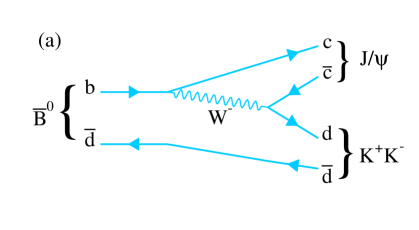
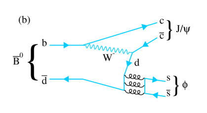
Figure 1: Feynman diagrams for (a) $\kern 1.61993pt\overline{\kern-1.61993ptB}{}^{0}\rightarrow{J\mskip-3.0mu/\mskip-2.0mu\psi\mskip 2.0mu}K^{+}K^{-}$, and (b) $\kern 1.61993pt\overline{\kern-1.61993ptB}{}^{0}\rightarrow{J\mskip-3.0mu/\mskip-2.0mu\psi\mskip 2.0mu}\phi$.

The formation of a $\phi$ meson can occur in this decay either via $\omega-\phi$ mixing which requires a small $d\overline{}d$ component in its wave function; or via a strong coupling such as shown in Fig. 1(b), which illustrates tri-gluon exchange. Gronau and Rosner predicted that the dominant contribution is via $\omega-\phi$ mixing at the order of $10^{-7}$ [4].

In this paper, we report on a measurement of the branching fraction of the decay $\kern 1.79993pt\overline{\kern-1.79993ptB}{}^{0}\rightarrow{J\mskip-3.0mu/\mskip-2.0mu\psi\mskip 2.0mu}K^{+}K^{-}$. A modified Dalitz plot analysis of the final state is performed to study the resonant and nonresonant structures in the $K^{+}\kern-1.60004ptK^{-}$ mass spectrum using the ${J\mskip-3.0mu/\mskip-2.0mu\psi\mskip 2.0mu}K^{+}$ and $K^{+}\kern-1.60004ptK^{-}$ mass spectra and decay angular distributions. This differs from a classical Dalitz plot analysis [5] because the ${J\mskip-3.0mu/\mskip-2.0mu\psi\mskip 2.0mu}$ meson has spin one, so its three helicity amplitudes must be considered. In addition, a search for the decay $\kern 1.79993pt\overline{\kern-1.79993ptB}{}^{0}\rightarrow{J\mskip-3.0mu/\mskip-2.0mu\psi\mskip 2.0mu}\phi$ is performed.

2 Data sample and detector

The data sample consists of $1.0~{}\rm fb^{-1}$ of integrated luminosity collected with the LHCb detector [6] using $pp$ collisions at a center-of-mass energy of 7 TeV. The LHCb detector is a single-arm forward spectrometer covering the pseudorapidity range $2<\eta<5$, designed for the study of particles containing $b$ or $c$ quarks. The detector includes a high precision tracking system consisting of a silicon-strip vertex detector surrounding the $pp$ interaction region, a large-area silicon-strip detector located upstream of a dipole magnet with a bending power of about $4{\rm\,Tm}$, and three stations of silicon-strip detectors and straw drift tubes placed downstream. The combined tracking system has momentum resolution $\Delta p/p$ that varies from 0.4% at 5$\mathrm{\,Ge\kern-1.00006ptV}$ to 0.6% at 100$\mathrm{\,Ge\kern-1.00006ptV}$. The impact parameter (IP) is defined as the minimum distance of approach of the track with respect to the primary vertex. For tracks with large transverse momentum, $p_{\rm T}$, with respect to the proton beam direction, the IP resolution is approximately 20$\,\upmu\rm m$. Charged hadrons are identified using two ring-imaging Cherenkov detectors (RICH) [7]. Photon, electron and hadron candidates are identified by a calorimeter system consisting of scintillating-pad and pre-shower detectors, an electromagnetic calorimeter and a hadronic calorimeter. Muons are identified by a system composed of alternating layers of iron and multiwire proportional chambers [8]. The trigger consists of a hardware stage, based on information from the calorimeter and muon systems, followed by a software stage which applies a full event reconstruction [9].

In the simulation, $pp$ collisions are generated using Pythia 6.4 [10] with a specific LHCb configuration [11]. Decays of hadrons are described by EvtGen [12] in which final state radiation is generated using Photos [13]. The interaction of the generated particles with the detector and its response are implemented using the Geant4 toolkit [14, *Agostinelli:2002hh] as described in Ref. [16].

3 Event selection

The reconstruction of $\kern 1.79993pt\overline{\kern-1.79993ptB}{}^{0}\rightarrow{J\mskip-3.0mu/\mskip-2.0mu\psi\mskip 2.0mu}K^{+}\kern-1.60004ptK^{-}$ candidates proceeds by finding ${J\mskip-3.0mu/\mskip-2.0mu\psi\mskip 2.0mu}\rightarrow\mu^{+}\mu^{-}$ candidates and combining them with a pair of oppositely charged kaons. Good quality of the reconstructed tracks is ensured by requiring the $\chi^{2}/\rm ndf$ of the track fit to be less than 4, where ndf is the number of degrees of freedom of the fit. To form a ${J\mskip-3.0mu/\mskip-2.0mu\psi\mskip 2.0mu}\rightarrow\mu^{+}\mu^{-}$ candidate, particles identified as muons of opposite charge are required to have $p_{\rm T}$ greater than 500 $\mathrm{\,Me\kern-1.00006ptV}$ each, and form a vertex with fit $\chi^{2}$ less than 16. Only candidates with a dimuon invariant mass between $-48$ $\mathrm{\,Me\kern-1.00006ptV}$ and $+43$ $\mathrm{\,Me\kern-1.00006ptV}$ relative to the observed ${J\mskip-3.0mu/\mskip-2.0mu\psi\mskip 2.0mu}$ peak are selected, where the r.m.s. resolution is 13.4 MeV. The requirement is asymmetric due to final state electromagnetic radiation. The $\mu^{+}\mu^{-}$ combinations are then constrained to the ${J\mskip-3.0mu/\mskip-2.0mu\psi\mskip 2.0mu}$ mass [17] for subsequent use in event reconstruction.

Each kaon candidate is required to have $p_{\rm T}$ greater than 250 $\mathrm{\,Me\kern-1.00006ptV}$ and $\chi^{2}_{\rm IP}>9$, where the $\chi^{2}_{\rm IP}$ is computed as the difference between the $\chi^{2}$ of the primary vertex reconstructed with and without the considered track. In addition, the scalar sum of their transverse momenta, $\mbox{$p_{\rm T}$}(K^{+})+\mbox{$p_{\rm T}$}(K^{-})$, must be greater than 900 $\mathrm{\,Me\kern-1.00006ptV}$. The $K^{+}\kern-1.60004ptK^{-}$ candidates are required to form a vertex with a $\chi^{2}$ less than 10 for one degree of freedom. We identify the hadron species of each track from the difference DLL($h_{1}-h_{2}$) between logarithms of the likelihoods associated with the two hypotheses $h_{1}$ and $h_{2}$, as provided by the RICH detector. Two criteria are used, with the “loose” criterion corresponding to DLL$(K-\pi)>0$, while “tight” criterion requires DLL$(K-\pi)>10$ and DLL$(K-p)>-3$. Unless stated otherwise, we use the tight criterion for the kaon selection.

The $\kern 1.79993pt\overline{\kern-1.79993ptB}{}^{0}$ candidate should have vertex fit $\chi^{2}$ less than 50 for five degrees of freedom and a $\chi^{2}_{\rm IP}$ with respect to the primary vertex less than 25. When more than one primary vertex is reconstructed, the one that gives the minimum $\chi^{2}_{\rm IP}$ is chosen. The $\kern 1.79993pt\overline{\kern-1.79993ptB}{}^{0}$ candidate must have a flight distance of more than 1.5 mm from the associated primary vertex. In addition, the angle between the combined momentum vector of the decay products and the vector formed from the position of the primary vertex to the decay vertex (pointing angle) is required to be smaller than $2.56^{\circ}$.

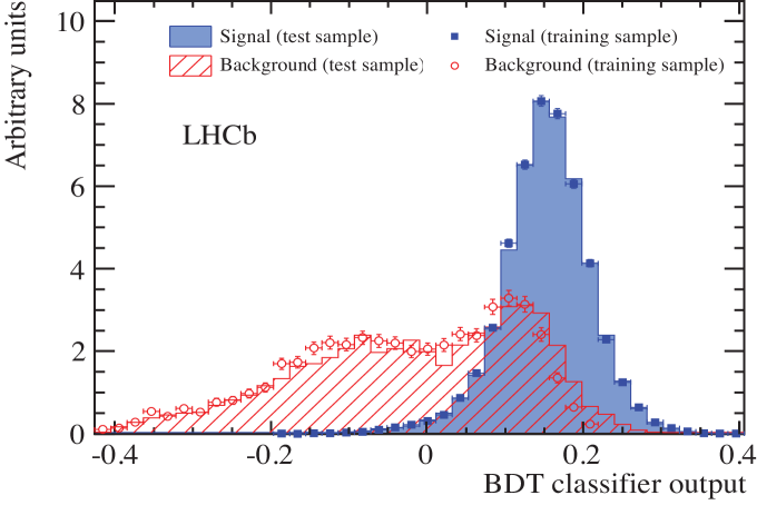
Figure 2: Distribution of the BDT classifier for both training and test samples of ${J\mskip-3.0mu/\mskip-2.0mu\psi\mskip 2.0mu}K^{+}\kern-1.44003ptK^{-}$ signal and background events. The signal samples are from simulation and the background samples are from data. The small difference between the background training and test samples is due to the fact that the sidebands used in the two cases are not identical.

Events satisfying the above criteria are further filtered using a multivariate classifier based on a Boosted Decision Tree (BDT) technique [18]. The BDT uses six variables that are chosen to provide separation between signal and background. The BDT variables are the minimum DLL($\mu-\pi$) of the $\mu^{+}$ and $\mu^{-}$, the minimum $p_{\rm T}$ of the $K^{+}$ and $K^{-}$, the minimum of the $\chi^{2}_{\rm IP}$ of the $K^{+}$ and $K^{-}$, the $\kern 1.79993pt\overline{\kern-1.79993ptB}{}^{0}$ vertex $\chi^{2}$, the $\kern 1.79993pt\overline{\kern-1.79993ptB}{}^{0}$ pointing angle, and the $\kern 1.79993pt\overline{\kern-1.79993ptB}{}^{0}$ flight distance. The BDT is trained on a simulated sample of $\kern 1.79993pt\overline{\kern-1.79993ptB}{}^{0}\rightarrow{J\mskip-3.0mu/\mskip-2.0mu\psi\mskip 2.0mu}K^{+}\kern-1.60004ptK^{-}$ signal events and a background data sample from the sideband $5180<m({J\mskip-3.0mu/\mskip-2.0mu\psi\mskip 2.0mu}K^{+}\kern-1.60004ptK^{-})<5230$ $\mathrm{\,Me\kern-1.00006ptV}$ of the $\kern 1.79993pt\overline{\kern-1.79993ptB}{}^{0}$ signal peak. The BDT is then tested on independent samples. The distributions of the output of the BDT classifier for signal and background are shown in Fig. 2. The final selection is optimized by maximizing $N_{S}/\sqrt{(N_{S}+N_{B})}$, where the expected signal yield $N_{S}$ and the expected background yield $N_{B}$ are estimated from the yields before applying the BDT, multiplied by the efficiencies associated to various values of the BDT selection as determined in test samples. The optimal selection is found to be $\rm BDT>0.1$, which has an $86\%$ signal efficiency and a $72\%$ background rejection rate.

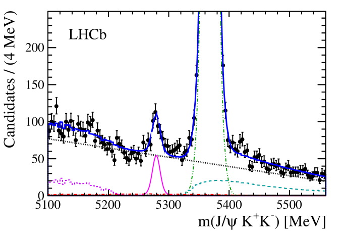
Figure 3: Invariant mass of ${J\mskip-3.0mu/\mskip-2.0mu\psi\mskip 2.0mu}K^{+}\kern-1.44003ptK^{-}$ combinations. The data are fitted with a sum of two Gaussian functions for each signal peak and several background components. The (magenta) solid double-Gaussian function centered at 5280 MeV is the $\kern 1.61993pt\overline{\kern-1.61993ptB}{}^{0}$ signal, the (black) dotted curve shows the combinatorial background, the (green) dashed-dot-dot curve shows the contribution of $\kern 1.61993pt\overline{\kern-1.61993ptB}{}^{0}_{s}\rightarrow{J\mskip-3.0mu/\mskip-2.0mu\psi\mskip 2.0mu}K^{+}\kern-1.44003ptK^{-}$ decays, the (violet) dashed shape is the $\kern 1.61993pt\overline{\kern-1.61993ptB}{}^{0}_{s}\rightarrow{J\mskip-3.0mu/\mskip-2.0mu\psi\mskip 2.0mu}K^{+}\pi^{0}K^{-}$ background, $\mathchar 28931\relax^{0}_{b}\rightarrow{J\mskip-3.0mu/\mskip-2.0mu\psi\mskip 2.0mu}pK^{-}$ and $\kern 1.61993pt\overline{\kern-1.61993ptB}{}^{0}\rightarrow{J\mskip-3.0mu/\mskip-2.0mu\psi\mskip 2.0mu}K^{-}\pi^{+}$ reflections are shown by (red) dot-dashed and (cyan) long dashed shapes, respectively and the (blue) solid curve is the total.

The invariant mass distribution of the selected ${J\mskip-3.0mu/\mskip-2.0mu\psi\mskip 2.0mu}K^{+}K^{-}$ combinations is shown in Fig. 3. Signal peaks are observed at both the $\kern 1.79993pt\overline{\kern-1.79993ptB}{}^{0}_{s}$ and $\kern 1.79993pt\overline{\kern-1.79993ptB}{}^{0}$ masses overlapping a smooth background. We model the $\kern 1.79993pt\overline{\kern-1.79993ptB}{}^{0}_{s}\rightarrow{J\mskip-3.0mu/\mskip-2.0mu\psi\mskip 2.0mu}K^{+}K^{-}$ signal by a sum of two Gaussian functions with common mean; the mass resolution is found to be 6.2 MeV. The shape of the $\kern 1.79993pt\overline{\kern-1.79993ptB}{}^{0}\rightarrow{J\mskip-3.0mu/\mskip-2.0mu\psi\mskip 2.0mu}K^{+}K^{-}$ signal component is constrained to be the same as that of the $\kern 1.79993pt\overline{\kern-1.79993ptB}{}^{0}_{s}$ signal. The background components include the combinatorial background, a contribution from the $\kern 1.79993pt\overline{\kern-1.79993ptB}{}^{0}_{s}\rightarrow{J\mskip-3.0mu/\mskip-2.0mu\psi\mskip 2.0mu}K^{+}\pi^{0}K^{-}$ decay, and reflections from $\mathchar 28931\relax^{0}_{b}\rightarrow{J\mskip-3.0mu/\mskip-2.0mu\psi\mskip 2.0mu}pK^{-}$ and $\kern 1.79993pt\overline{\kern-1.79993ptB}{}^{0}\rightarrow{J\mskip-3.0mu/\mskip-2.0mu\psi\mskip 2.0mu}K^{-}\pi^{+}$ decays, where a proton in the former and a pion in the latter are misidentified as a kaon. The combinatorial background is described by a linear function. The shape of the $\kern 1.79993pt\overline{\kern-1.79993ptB}{}^{0}_{s}\rightarrow{J\mskip-3.0mu/\mskip-2.0mu\psi\mskip 2.0mu}K^{+}\pi^{0}K^{-}$ background is taken from simulation, generated uniformly in phase space, with its yield allowed to vary. The reflection shapes are also taken from simulations, while the yields are Gaussian constrained in the global fit to the expected values estimated by measuring the number of $\mathchar 28931\relax^{0}_{b}$ and $\kern 1.79993pt\overline{\kern-1.79993ptB}{}^{0}$ candidates in the control region $25-300$ MeV above the $\kern 1.79993pt\overline{\kern-1.79993ptB}{}^{0}_{s}$ mass peak. The shape of the $\mathchar 28931\relax^{0}_{b}\rightarrow{J\mskip-3.0mu/\mskip-2.0mu\psi\mskip 2.0mu}pK^{-}$ reflection is determined from the simulation weighted according to the $m(pK^{-})$ distribution obtained in Ref. [19], while the simulations of $\kern 1.79993pt\overline{\kern-1.79993ptB}{}^{0}\rightarrow{J\mskip-3.0mu/\mskip-2.0mu\psi\mskip 2.0mu}\kern 1.99997pt\overline{\kern-1.99997ptK}{}^{*0}(892)$ and $\kern 1.79993pt\overline{\kern-1.79993ptB}{}^{0}\rightarrow{J\mskip-3.0mu/\mskip-2.0mu\psi\mskip 2.0mu}\kern 1.99997pt\overline{\kern-1.99997ptK}{}^{*}_{2}(1430)$ decays are used to study the shape of the $\kern 1.79993pt\overline{\kern-1.79993ptB}{}^{0}\rightarrow{J\mskip-3.0mu/\mskip-2.0mu\psi\mskip 2.0mu}K^{-}\pi^{+}$ reflection. From the fit, we extract $228\pm 27$ $\kern 1.79993pt\overline{\kern-1.79993ptB}{}^{0}$ signal candidates together with $545\pm 14$ combinatorial background and $20\pm 4$ $\mathchar 28931\relax^{0}_{b}\rightarrow{J\mskip-3.0mu/\mskip-2.0mu\psi\mskip 2.0mu}pK^{-}$ reflection candidates within $\pm 20$ MeV of the $\kern 1.79993pt\overline{\kern-1.79993ptB}{}^{0}$ mass peak.

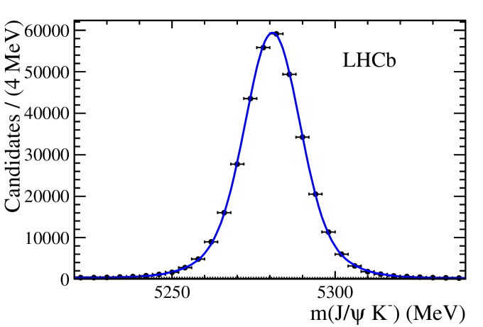
Figure 4: Fit to the invariant mass spectrum of ${J\mskip-3.0mu/\mskip-2.0mu\psi\mskip 2.0mu}K^{-}$ combinations. The (blue) solid curve is the total and the (black) dotted line shows the combinatorial background.

We use the decay $B^{-}\rightarrow{J\mskip-3.0mu/\mskip-2.0mu\psi\mskip 2.0mu}K^{-}$ as the normalization channel for branching fraction determinations. The selection criteria are similar to those used for the ${J\mskip-3.0mu/\mskip-2.0mu\psi\mskip 2.0mu}K^{+}\kern-1.60004ptK^{-}$ final state, except for particle identification requirements since here the loose kaon identification criterion is used. Similar variables are used for the BDT, except that the variables describing the combination of $K^{+}$ and $K^{-}$ in the ${J\mskip-3.0mu/\mskip-2.0mu\psi\mskip 2.0mu}K^{+}\kern-1.60004ptK^{-}$ final state are replaced by the ones that describe the $K^{-}$ meson. The BDT training uses $B^{-}\rightarrow{J\mskip-3.0mu/\mskip-2.0mu\psi\mskip 2.0mu}K^{-}$ simulated events as signal and data in the sideband region $5400<m({J\mskip-3.0mu/\mskip-2.0mu\psi\mskip 2.0mu}K^{-})<5450$ $\mathrm{\,Me\kern-1.00006ptV}$ as background. The resulting invariant mass distribution of the ${J\mskip-3.0mu/\mskip-2.0mu\psi\mskip 2.0mu}K^{-}$ candidates satisfying BDT classifier output greater than $0.1$ is shown in Fig. 4. The signal is fit with a sum of two Gaussian functions with common mean and the combinatorial background is fit with a linear function. There are $322\,696\pm 596$ signal and $3484\pm 88$ background candidates within $\pm 20$ MeV of the $B^{-}$ peak.

4 Analysis formalism

The decay $\kern 1.79993pt\overline{\kern-1.79993ptB}{}^{0}\rightarrow{J\mskip-3.0mu/\mskip-2.0mu\psi\mskip 2.0mu}K^{+}K^{-}$ followed by ${J\mskip-3.0mu/\mskip-2.0mu\psi\mskip 2.0mu}\rightarrow\mu^{+}\mu^{-}$ can be described by four variables. These are taken to be the invariant mass squared of ${J\mskip-3.0mu/\mskip-2.0mu\psi\mskip 2.0mu}K^{+}$, $s_{12}\equiv m^{2}({J\mskip-3.0mu/\mskip-2.0mu\psi\mskip 2.0mu}K^{+})$, the invariant mass squared of $K^{+}K^{-}$, $s_{23}\equiv m^{2}(K^{+}K^{-})$, the ${J\mskip-3.0mu/\mskip-2.0mu\psi\mskip 2.0mu}$ helicity angle, $\theta_{{J\mskip-3.0mu/\mskip-2.0mu\psi\mskip 2.0mu}}$, which is the angle of the $\mu^{+}$ in the ${J\mskip-3.0mu/\mskip-2.0mu\psi\mskip 2.0mu}$ rest frame with respect to the ${J\mskip-3.0mu/\mskip-2.0mu\psi\mskip 2.0mu}$ direction in the $\kern 1.79993pt\overline{\kern-1.79993ptB}{}^{0}$ rest frame, and $\chi$, the angle between the ${J\mskip-3.0mu/\mskip-2.0mu\psi\mskip 2.0mu}$ and $K^{+}K^{-}$ decay planes in the $\kern 1.79993pt\overline{\kern-1.79993ptB}{}^{0}$ rest frame. Our approach is similar to that used in the LHCb analyses of $\kern 1.79993pt\overline{\kern-1.79993ptB}{}^{0}_{s}\rightarrow{J\mskip-3.0mu/\mskip-2.0mu\psi\mskip 2.0mu}\pi^{+}\pi^{-}$ [1], $\kern 1.79993pt\overline{\kern-1.79993ptB}{}^{0}_{s}\rightarrow{J\mskip-3.0mu/\mskip-2.0mu\psi\mskip 2.0mu}K^{+}\kern-1.60004ptK^{-}$ [2] and $\kern 1.79993pt\overline{\kern-1.79993ptB}{}^{0}\rightarrow{J\mskip-3.0mu/\mskip-2.0mu\psi\mskip 2.0mu}\pi^{+}\pi^{-}$ [3], where a modified Dalitz plot analysis of the final state is performed after integrating over the angular variable $\chi$.

To study the resonant structures of the decay $\kern 1.79993pt\overline{\kern-1.79993ptB}{}^{0}\rightarrow{J\mskip-3.0mu/\mskip-2.0mu\psi\mskip 2.0mu}K^{+}\kern-1.60004ptK^{-}$, we use candidates with invariant mass within $\pm 20$ MeV of the observed $\kern 1.79993pt\overline{\kern-1.79993ptB}{}^{0}$ mass peak. The invariant mass squared of $K^{+}\kern-1.60004ptK^{-}$ versus ${J\mskip-3.0mu/\mskip-2.0mu\psi\mskip 2.0mu}K^{+}$ is shown in Fig. 5.

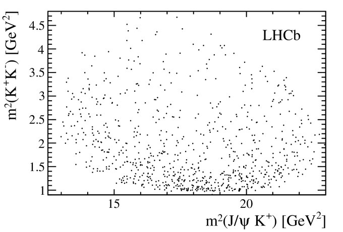
Figure 5: Distribution of $m^{2}(K^{+}\kern-1.44003ptK^{-})$ versus $m^{2}({J\mskip-3.0mu/\mskip-2.0mu\psi\mskip 2.0mu}K^{+})$ for ${J\mskip-3.0mu/\mskip-2.0mu\psi\mskip 2.0mu}K^{+}\kern-1.44003ptK^{-}$ candidates with mass within $\pm 20$ MeV of the $\kern 1.61993pt\overline{\kern-1.61993ptB}{}^{0}$ mass.

An excess of events is visible at low $K^{+}\kern-1.60004ptK^{-}$ mass, which could include both nonresonant and resonant contributions. Possible resonance candidates include $a_{0}(980)$, $f_{0}(980)$, $\phi$, $f_{0}(1370)$, $a_{0}(1450)$, or $f_{0}(1500)$ mesons. Because of the limited sample size, we perform the analysis including only the $a_{0}(980)$ and $f_{0}(980)$ resonances and nonresonant components.

In our previous analysis of $\kern 1.79993pt\overline{\kern-1.79993ptB}{}^{0}\rightarrow{J\mskip-3.0mu/\mskip-2.0mu\psi\mskip 2.0mu}\pi^{+}\pi^{-}$ decay [3], we did not see a statistically significant contribution of the $f_{0}(980)$ resonance. The branching fraction product was determined as

$$\mathcal{B}(\kern 1.79993pt\overline{\kern-1.79993ptB}{}^{0}\rightarrow{J\mskip-3.0mu/\mskip-2.0mu\psi\mskip 2.0mu}f_{0}(980),~{}f_{0}(980)\rightarrow\pi^{+}\pi^{-})=(6.1~{}^{+3.1}_{-2.0}~{}^{+1.7}_{-1.4})\times 10^{-7}.$$

Using this branching fraction product and the ratio of branching fractions,

$$\mathcal{R}=\frac{\mathcal{B}(f_{0}(980)\rightarrow K^{+}\kern-1.60004ptK^{-})}{\mathcal{B}(f_{0}(980)\rightarrow\pi^{+}\pi^{-})}=0.35^{+0.15}_{-0.14},$$ (1)

determined from an average of the BES [20] and BaBar [21] measurements, we estimate the expected yield of $\kern 1.79993pt\overline{\kern-1.79993ptB}{}^{0}\rightarrow{J\mskip-3.0mu/\mskip-2.0mu\psi\mskip 2.0mu}f_{0}(980)$ with $f_{0}(980)\rightarrow K^{+}\kern-1.60004ptK^{-}$ as

$$N(\kern 1.79993pt\overline{\kern-1.79993ptB}{}^{0}\rightarrow{J\mskip-3.0mu/\mskip-2.0mu\psi\mskip 2.0mu}f_{0}(980),~{}f_{0}(980)\rightarrow K^{+}\kern-1.60004ptK^{-})=20^{+14}_{-11}.$$

Although the $f_{0}(980)$ meson is easier to detect in its $\pi^{+}\pi^{-}$ final state than in $K^{+}\kern-1.60004ptK^{-}$, the presence of the $f_{0}(980)$ resonance was not established in the $\kern 1.79993pt\overline{\kern-1.79993ptB}{}^{0}\rightarrow{J\mskip-3.0mu/\mskip-2.0mu\psi\mskip 2.0mu}\pi^{+}\pi^{-}$ decay [3], despite some positive indication. Therefore, we test for two models: one that includes the $f_{0}(980)$ resonance with fixed amplitude strength corresponding to the expected yield and label it as “default” and the other without the $f_{0}(980)$ resonance. The latter is called “alternate”.

4.1 The model for $\kern 1.79993pt\overline{\kern-1.79993ptB}{}^{0}\rightarrow{J\mskip-3.0mu/\mskip-2.0mu\psi\mskip 2.0mu}K^{+}K^{-}$

The overall probability density function (PDF) given by the sum of signal, $S$, and background functions, $B$, is

$$F(s_{12},s_{23},\theta_{{J\mskip-3.0mu/\mskip-2.0mu\psi\mskip 2.0mu}}) = \frac{1-f_{\rm com}-f_{\rm refl}}{{\cal{N}}_{\rm sig}}\varepsilon(s_{12},s_{23},\theta_{{J\mskip-3.0mu/\mskip-2.0mu\psi\mskip 2.0mu}})S(s_{12},s_{23},\theta_{{J\mskip-3.0mu/\mskip-2.0mu\psi\mskip 2.0mu}})$$

$$+ B(s_{12},s_{23},\theta_{{J\mskip-3.0mu/\mskip-2.0mu\psi\mskip 2.0mu}}),$$

where the background is the sum of combinatorial background, $C$, and reflection, $R$, functions,

$$B(s_{12},s_{23},\theta_{{J\mskip-3.0mu/\mskip-2.0mu\psi\mskip 2.0mu}})=\frac{f_{\rm com}}{{\cal{N}}_{\rm com}}C(s_{12},s_{23},\theta_{{J\mskip-3.0mu/\mskip-2.0mu\psi\mskip 2.0mu}})+\frac{f_{\rm refl}}{{\cal{N}}_{\rm refl}}R(s_{12},s_{23},\theta_{{J\mskip-3.0mu/\mskip-2.0mu\psi\mskip 2.0mu}}),$$ (3)

and $f_{\rm com}$ and $f_{\rm refl}$ are the fractions of the combinatorial background and reflection, respectively, in the fitted region, and $\varepsilon$ is the detection efficiency. The fractions $f_{\rm com}$ and $f_{\rm refl}$, obtained from the mass fit, are fixed for the subsequent analysis.

The normalization factors are given by

$${\cal{N}}_{\rm sig} = \int\!\varepsilon(s_{12},s_{23},\theta_{{J\mskip-3.0mu/\mskip-2.0mu\psi\mskip 2.0mu}})S(s_{12},s_{23},\theta_{{J\mskip-3.0mu/\mskip-2.0mu\psi\mskip 2.0mu}})\,ds_{12}ds_{23}d\cos\theta_{{J\mskip-3.0mu/\mskip-2.0mu\psi\mskip 2.0mu}},$$

$${\cal{N}}_{\rm com} = \int\!C(s_{12},s_{23},\theta_{{J\mskip-3.0mu/\mskip-2.0mu\psi\mskip 2.0mu}})\,ds_{12}ds_{23}d\cos\theta_{{J\mskip-3.0mu/\mskip-2.0mu\psi\mskip 2.0mu}},$$ (4)

$${\cal{N}}_{\rm refl} = \int\!R(s_{12},s_{23},\theta_{{J\mskip-3.0mu/\mskip-2.0mu\psi\mskip 2.0mu}})\,ds_{12}ds_{23}d\cos\theta_{{J\mskip-3.0mu/\mskip-2.0mu\psi\mskip 2.0mu}}.$$

The expression for the signal function, $S(s_{12},s_{23},\theta_{{J\mskip-3.0mu/\mskip-2.0mu\psi\mskip 2.0mu}})$, amplitude for the nonresonant process and other details of the fitting procedure are the same as used in the analysis described in Refs. [1, 2, 3]. The amplitudes for the $a_{0}(980)$ and $f_{0}(980)$ resonances are described below.

The main decay channels of the $a_{0}(980)$ (or $f_{0}(980)$) resonance are $\eta\pi$ (or $\pi\pi$) and $K\kern 1.99997pt\overline{\kern-1.99997ptK}{}$, with the former being the larger [17]. Both the $a_{0}(980)$ and the $f_{0}(980)$ resonances are very close to the $K\kern 1.99997pt\overline{\kern-1.99997ptK}{}$ threshold, which can strongly influence the resonance shape. To take this complication into account, we follow the widely accepted prescription proposed by Flatté [22], based on the coupled channels $\eta\pi^{0}$ (or $\pi\pi$) and $KK$. The Flatté mass shapes are parametrized as

$$A^{a_{0}}_{R}(s_{23})=\frac{1}{m_{R}^{2}-s_{23}-i(g_{\eta\pi}^{2}\rho_{\eta\pi}+g_{KK}^{2}\rho_{KK})}$$ (5)

for the $a_{0}(980)$ resonance, and

$$A^{f_{0}}_{R}(s_{23})=\frac{1}{m_{R}^{2}-s_{23}-im_{R}(g_{\pi\pi}\rho_{\pi\pi}+g_{KK}\rho_{KK})}$$ (6)

for the $f_{0}(980)$ resonance. In both cases, $m_{R}$ refers to the pole mass of the resonance. The constants $g_{\eta\pi}$ (or $g_{\pi\pi}$) and $g_{KK}$ are the coupling strengths of $a_{0}(980)$ (or $f_{0}(980)$) to $\eta\pi^{0}$ (or $\pi\pi$) and $KK$ final states, respectively. The $\rho$ factors are given by the Lorentz-invariant phase space

$$\rho_{\eta\pi} = \sqrt{\left(1-\left(\frac{m_{\eta}-m_{\pi^{0}}}{\sqrt{s_{23}}}\right)^{2}\right)\left(1-\left(\frac{m_{\eta}+m_{\pi^{0}}}{\sqrt{s_{23}}}\right)^{2}\right)},$$ (7)

$$\rho_{\pi\pi} = \frac{2}{3}\sqrt{1-\frac{4m^{2}_{\pi^{\pm}}}{s_{23}}}+\frac{1}{3}\sqrt{1-\frac{4m^{2}_{\pi^{0}}}{s_{23}}},$$ (8)

$$\rho_{KK} = \frac{1}{2}\sqrt{1-\frac{4m^{2}_{K^{\pm}}}{s_{23}}}+\frac{1}{2}\sqrt{1-\frac{4m^{2}_{K^{0}}}{s_{23}}}.$$ (9)

The parameters for the $a_{0}(980)$ lineshape are fixed in the fit as determined by the Crystal Barrel experiment [23]. The parameters are $m_{R}=999\pm 2~{}\rm MeV$, $g_{\eta\pi}=324\pm 15~{}\rm MeV$ and $g^{2}_{KK}/g^{2}_{\eta\pi}=1.03\pm 0.14$. The parameters for $f_{0}(980)$ are also fixed to the values $m_{R}=939.9\pm 6.3$ MeV, $g_{\pi\pi}=199\pm 30$ MeV and $g_{KK}/g_{\pi\pi}=3.0\pm 0.3$, obtained from our previous analysis of $\kern 1.79993pt\overline{\kern-1.79993ptB}{}^{0}_{s}\rightarrow{J\mskip-3.0mu/\mskip-2.0mu\psi\mskip 2.0mu}\pi^{+}\pi^{-}$ decay [1].

4.2 Detection efficiency

The detection efficiency is determined from a sample of $10^{6}$ $\kern 1.79993pt\overline{\kern-1.79993ptB}{}^{0}\rightarrow{J\mskip-3.0mu/\mskip-2.0mu\psi\mskip 2.0mu}K^{+}\kern-1.60004ptK^{-}$ simulated events that are generated uniformly in phase space. The distributions of the generated $\kern 1.79993pt\overline{\kern-1.79993ptB}{}^{0}$ meson are weighted according to the $p$ and $p_{\rm T}$ distributions in order to match those observed in data. We also correct for the differences between the simulated kaon detection efficiencies and the measured ones determined by using a sample of $D^{*+}\rightarrow\pi^{+}(D^{0}\rightarrow K^{-}\pi^{+})$ events.

The efficiency is described in terms of the analysis variables. Both $s_{12}$ and $s_{13}$ range from $12.5~{}\rm GeV^{2}$ to $23.0~{}\rm GeV^{2}$, where $s_{13}$ is defined below, and thus are centered at $s_{0}=17.75$ GeV². We model the detection efficiency using the dimensionless symmetric Dalitz plot observables

$$x=(s_{12}-s_{0})/(1~{}{\rm GeV}^{2})~{}~{}~{}~{}{\rm and}~{}~{}~{}~{}y=(s_{13}-s_{0})/(1~{}{\rm GeV}^{2}),$$ (10)

and the angular variable $\theta_{{J\mskip-3.0mu/\mskip-2.0mu\psi\mskip 2.0mu}}$. The observables $s_{12}$ and $s_{13}$ are related to $s_{23}$ as

$$s_{12}+s_{13}+s_{23}=m^{2}_{B}+m^{2}_{{J\mskip-3.0mu/\mskip-2.0mu\psi\mskip 2.0mu}}+m^{2}_{K^{+}}+m^{2}_{K^{-}}~{}.$$ (11)

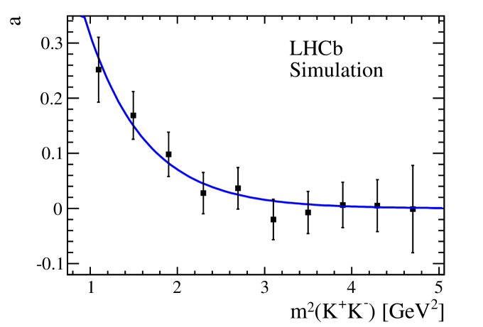
Figure 6: Exponential fit to the acceptance parameter $a(s_{23})$.

To parametrize this efficiency, we fit the $\cos\theta_{{J\mskip-3.0mu/\mskip-2.0mu\psi\mskip 2.0mu}}$ distributions of the $\kern 1.79993pt\overline{\kern-1.79993ptB}{}^{0}\rightarrow{J\mskip-3.0mu/\mskip-2.0mu\psi\mskip 2.0mu}K^{+}\kern-1.60004ptK^{-}$ simulated sample in bins of $s_{23}$ with the function

$$\varepsilon_{2}(s_{23},\theta_{{J\mskip-3.0mu/\mskip-2.0mu\psi\mskip 2.0mu}})=\frac{1+a(s_{23})\cos^{2}\theta_{{J\mskip-3.0mu/\mskip-2.0mu\psi\mskip 2.0mu}}}{2+2a(s_{23})/3},$$ (12)

where $a$ is a function of $s_{23}$. The resulting distribution, shown in Fig. 6, is described by an exponential function

$$a(s_{23})=\exp(a_{1}+a_{2}s_{23}),$$ (13)

where $a_{1}$ and $a_{2}$ are constant parameters. Equation (12) is normalized to one when integrated over $\cos\theta_{{J\mskip-3.0mu/\mskip-2.0mu\psi\mskip 2.0mu}}$. The efficiency as a function of $\cos\theta_{{J\mskip-3.0mu/\mskip-2.0mu\psi\mskip 2.0mu}}$ also depends on $s_{23}$, and is observed to be independent of $s_{12}$. Therefore, the detection efficiency can be expressed as

$$\varepsilon(s_{12},s_{23},\theta_{{J\mskip-3.0mu/\mskip-2.0mu\psi\mskip 2.0mu}})=\varepsilon_{1}(x,y)\times\varepsilon_{2}(s_{23},\theta_{{J\mskip-3.0mu/\mskip-2.0mu\psi\mskip 2.0mu}}).$$ (14)

After integrating over $\cos\theta_{{J\mskip-3.0mu/\mskip-2.0mu\psi\mskip 2.0mu}}$, Eq. (14) becomes

$$\int_{-1}^{+1}\varepsilon(s_{12},s_{23},\theta_{{J\mskip-3.0mu/\mskip-2.0mu\psi\mskip 2.0mu}})d\cos\theta_{{J\mskip-3.0mu/\mskip-2.0mu\psi\mskip 2.0mu}}=\varepsilon_{1}(x,y).$$ (15)

and is modeled by a symmetric fourth-order polynomial function given by

$$\varepsilon_{1}(x,y) = 1+\epsilon^{\prime}_{1}(x+y)+\epsilon^{\prime}_{2}(x+y)^{2}+\epsilon^{\prime}_{3}xy+\epsilon^{\prime}_{4}(x+y)^{3}+\epsilon^{\prime}_{5}xy(x+y)$$ (16)

$$+\epsilon^{\prime}_{6}(x+y)^{4}+\epsilon^{\prime}_{7}xy(x+y)^{2}+\epsilon^{\prime}_{8}x^{2}y^{2},$$

where the $\epsilon^{\prime}_{i}$ are fit parameters.

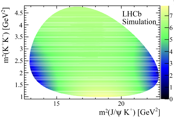
Figure 7: Parametrized detection efficiency as a function of $m^{2}(K^{+}\kern-1.44003ptK^{-})$ versus $m^{2}({J\mskip-3.0mu/\mskip-2.0mu\psi\mskip 2.0mu}K^{+})$. The $z$-axis scale is arbitrary.

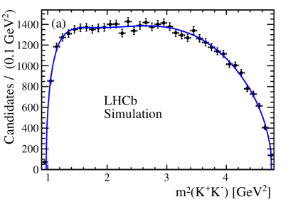
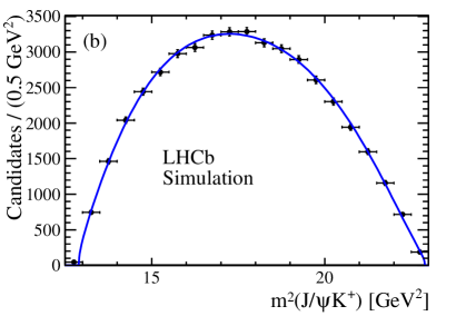
Figure 8: Projections of (a) $m^{2}(K^{+}\kern-1.44003ptK^{-})$ and (b) $m^{2}({J\mskip-3.0mu/\mskip-2.0mu\psi\mskip 2.0mu}K^{+})$ of the simulated Dalitz plot used to measure the efficiency parameters. The points represent the simulated event distributions, and the curves the projections of the polynomial fit.

Figure 7 shows the polynomial function obtained from a fit to the Dalitz plot distributions of simulated events. The projections of the fit describe the efficiency well as can be seen in Fig. 8.

4.3 Background composition

To parametrize the combinatorial background, we use the $\kern 1.79993pt\overline{\kern-1.79993ptB}{}^{0}$ mass sidebands, defined as the regions from 35 MeV to 60 MeV on the lower side and 25 MeV to 40 MeV on the upper side of the $\kern 1.79993pt\overline{\kern-1.79993ptB}{}^{0}$ mass peak. The shape of the combinatorial background is found to be

$$C(s_{12},s_{23},\theta_{{J\mskip-3.0mu/\mskip-2.0mu\psi\mskip 2.0mu}})=\left[C_{1}(s_{12},s_{23})\frac{P_{B}}{m_{B}}+\frac{c_{0}}{(m^{2}_{0}-s_{23})^{2}+m^{2}_{0}\Gamma_{0}^{2}}\right]\times\left(1+\alpha\cos^{2}\theta_{{J\mskip-3.0mu/\mskip-2.0mu\psi\mskip 2.0mu}}\right),$$ (17)

with $C_{1}(s_{12},s_{23})$ parametrized as

$$C_{1}(s_{12},s_{23})=1+c_{1}(x+y)+c_{2}(x+y)^{2}+c_{3}xy+c_{4}(x+y)^{3}+c_{5}xy(x+y),$$ (18)

where $P_{B}$ is the magnitude of the ${J\mskip-3.0mu/\mskip-2.0mu\psi\mskip 2.0mu}$ three-momentum in the $\kern 1.79993pt\overline{\kern-1.79993ptB}{}^{0}$ rest frame, $m_{B}$ is the known $\kern 1.79993pt\overline{\kern-1.79993ptB}{}^{0}$ mass, and $c_{i}$, $m_{0}$, $\Gamma_{0}$ and $\alpha$ are the model parameters. The variables $x$ and $y$ are defined in Eq. (10).

Figure 9 shows the invariant mass squared projections from an unbinned likelihood fit to the sidebands. The value of $\alpha$ is determined by fitting the $\cos\theta_{{J\mskip-3.0mu/\mskip-2.0mu\psi\mskip 2.0mu}}$ distribution of the combinatorial background sample, as shown in Fig. 10, with a function of the form $1+\alpha\cos^{2}\theta_{{J\mskip-3.0mu/\mskip-2.0mu\psi\mskip 2.0mu}}$, yielding $\alpha=-0.38\pm 0.10$.

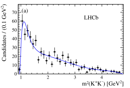
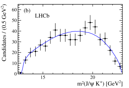
Figure 9: Invariant mass squared projections of (a) $K^{+}K^{-}$, and (b) ${J\mskip-3.0mu/\mskip-2.0mu\psi\mskip 2.0mu}K^{+}$ from the Dalitz plot of candidates in the $\kern 1.61993pt\overline{\kern-1.61993ptB}{}^{0}$ mass sidebands, with fit projection overlaid.

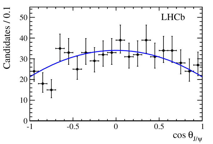
Figure 10: Distribution of $\cos\theta_{{J\mskip-3.0mu/\mskip-2.0mu\psi\mskip 2.0mu}}$ from the $\kern 1.61993pt\overline{\kern-1.61993ptB}{}^{0}$ mass sidebands, fitted with the function $1+\alpha\cos^{2}\theta_{{J\mskip-3.0mu/\mskip-2.0mu\psi\mskip 2.0mu}}$.

The reflection background is parametrized as

$$R(s_{12},s_{23},\theta_{{J\mskip-3.0mu/\mskip-2.0mu\psi\mskip 2.0mu}})=R_{1}(s_{12},s_{23})\times\left(1+\beta\cos^{2}\theta_{{J\mskip-3.0mu/\mskip-2.0mu\psi\mskip 2.0mu}}\right),$$ (19)

where $R_{1}(s_{12},s_{23})$ is modeled using the simulation of $\mathchar 28931\relax^{0}_{b}\rightarrow{J\mskip-3.0mu/\mskip-2.0mu\psi\mskip 2.0mu}pK^{-}$ decays weighted according to the $m(pK^{-})$ distribution obtained in Ref. [19]. The projections are shown in Fig. 11.

Figure 11: Projections of the reflection background in the variables (a) $m^{2}(K^{+}K^{-})$ and (b) $m^{2}({J\mskip-3.0mu/\mskip-2.0mu\psi\mskip 2.0mu}K^{+})$.

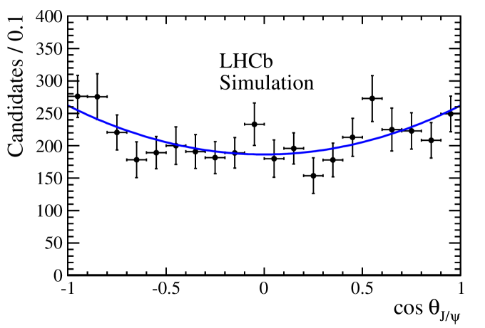
Figure 12: Distribution of $\cos\theta_{{J\mskip-3.0mu/\mskip-2.0mu\psi\mskip 2.0mu}}$ for the reflection background, fitted with the function $1+\beta\cos^{2}\theta_{{J\mskip-3.0mu/\mskip-2.0mu\psi\mskip 2.0mu}}$.

The ${J\mskip-3.0mu/\mskip-2.0mu\psi\mskip 2.0mu}$ helicity-dependent part of the reflection background parametrization is modeled as $1+\beta\cos^{2}\theta_{{J\mskip-3.0mu/\mskip-2.0mu\psi\mskip 2.0mu}}$, where the parameter $\beta=0.40\pm 0.08$ is obtained from a fit to the simulated $\cos\theta_{{J\mskip-3.0mu/\mskip-2.0mu\psi\mskip 2.0mu}}$ distribution of the same sample, shown in Fig. 12.

4.4 Fit results

An unbinned maximum likelihood fit is performed to extract the fit fractions and other physical parameters. Figure 13 shows the projection of $m^{2}(K^{+}\kern-1.60004ptK^{-})$ distribution for the default fit model. The $m^{2}({J\mskip-3.0mu/\mskip-2.0mu\psi\mskip 2.0mu}K^{+})$ and the $\cos\theta_{{J\mskip-3.0mu/\mskip-2.0mu\psi\mskip 2.0mu}}$ projections are displayed in Fig. 14. The background-subtracted $K^{+}\kern-1.60004ptK^{-}$ invariant mass spectrum for default and alternate fit models are shown in Fig. 15. Both the combinatorial background and the reflection components of the fit are subtracted from the data to obtain the background-subtracted distribution.

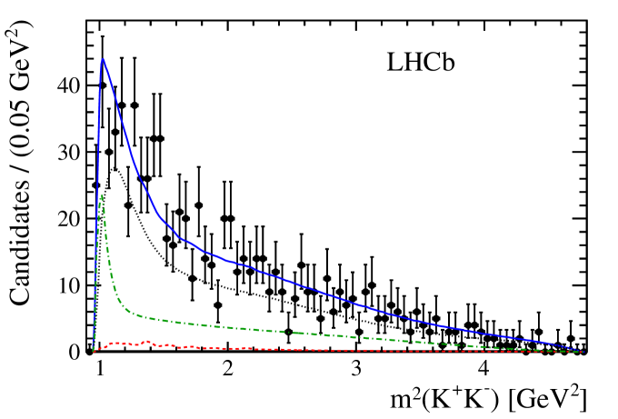
Figure 13: Dalitz plot fit projection of $m^{2}(K^{+}\kern-1.44003ptK^{-})$ in the signal region. The points with error bars are data, the (black) dotted curve shows the combinatorial background, the (red) dashed curve indicates the reflection from the misidentified $\mathchar 28931\relax^{0}_{b}\rightarrow{J\mskip-3.0mu/\mskip-2.0mu\psi\mskip 2.0mu}pK^{-}$ decays, the (green) dot-dashed curve is the signal, and the (blue) solid line represents the total.

Table 1: Fit fractions and phases of the contributing components. The components of the form $\rm X+Y$ are the interference terms. Note that, in the default model the $f_{0}(980)$ amplitude strength is fixed to the expected value. Poisson likelihood $\chi^{2}$ [24] is used to calculate the $\chi^{2}$.

Component	Default		Alternate
	Fit fraction (%)	Phase (∘)	Fit fraction (%)	Phase (∘)
$a_{0}(980)$	$19\pm 13$	$-10\pm 27$	$21\pm~{}8$	$-60\pm 26$
$f_{0}(980)$	$11\pm~{}5$	$-94\pm 45$	-	-
Nonresonant (NR)	$83\pm 37$	0 (fixed)	$85\pm 23$	0 (fixed)
$a_{0}(980)$ + NR	$-42\pm 25$	-	$-~{}6\pm 27$	-
$f_{0}(980)$ + NR	$32\pm 38$	-	-	-
$a_{0}(980)$ + $f_{0}(980)$	$-~{}2\pm 16$	-	-	-
$-\rm ln\mathcal{L}$	2940		2943
$\chi^{2}/\rm ndf$	1212/1406		1218/1407

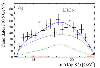
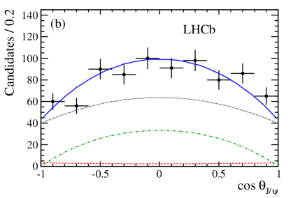
Figure 14: Dalitz plot fit projections of (a) $m^{2}({J\mskip-3.0mu/\mskip-2.0mu\psi\mskip 2.0mu}K^{+})$ and (b) $\cos\theta_{{J\mskip-3.0mu/\mskip-2.0mu\psi\mskip 2.0mu}}$ in the signal region. The points with error bars are data, the (black) dotted curve shows the combinatorial background, the (red) dashed curve indicates the reflection from the misidentified $\mathchar 28931\relax^{0}_{b}\rightarrow{J\mskip-3.0mu/\mskip-2.0mu\psi\mskip 2.0mu}pK^{-}$ decays, the (green) dot-dashed curve is the signal, and the (blue) solid line represents the total.

The fit fractions and the phases of the contributing components for both models are given in Table 1. Quoted uncertainties are statistical only, as determined from simulated experiments. We perform 500 experiments: each sample is generated according to the model PDF with input parameters from the results of the default fit. The correlations of the fitted parameters are also taken into account. For each experiment the fit fractions are calculated. The distributions of the obtained fit fractions are described by Gaussian functions. The r.m.s. widths of the Gaussian functions are taken as the statistical uncertainties on the corresponding parameters.

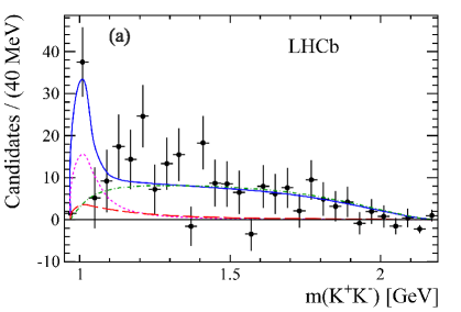
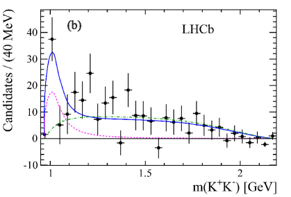
Figure 15: Background-subtracted $m(K^{+}\kern-1.44003ptK^{-})$ distributions for (a) default and, (b) alternate fit models in the signal region. The points with error bars are data, the (magenta) dashed curve shows the $a_{0}(980)$ resonance, the nonresonant contribution is shown by (green) dot-dashed curve and the (blue) solid curve represents the sum of $a_{0}(980)$, nonresonant and the interference between the two. The (red) long-dashed curve in (a) shows the $f_{0}(980)$ contribution.

The decay $\kern 1.79993pt\overline{\kern-1.79993ptB}{}^{0}\rightarrow{J\mskip-3.0mu/\mskip-2.0mu\psi\mskip 2.0mu}K^{+}\kern-1.60004ptK^{-}$ is dominated by the nonresonant S-wave components in the $K^{+}\kern-1.60004ptK^{-}$ system. The statistical significance of the $a_{0}(980)$ resonance is evaluated from the ratio, $\mathcal{L}_{a_{0}+f_{0}+\rm NR}/\mathcal{L}_{f_{0}+\rm NR}$, of the maximum likelihoods obtained from the fits with and without the resonance. The model with the resonance has two additional degrees of freedoms, corresponding to the amplitude strength and the phase. The quantity $2{\rm ln}(\mathcal{L}_{a_{0}+f_{0}+\rm NR}/\mathcal{L}_{f_{0}+\rm NR})$ is found to be 18.6, corresponding to a significance of 3.9 Gaussian standard deviations. The large statistical uncertainty in the $a_{0}(980)$ fit fraction in the default model is due to the presence of the $f_{0}(980)$ resonance that is allowed to interfere with the $a_{0}(980)$ resonance whose phase is highly correlated with the fit fraction. This uncertainty is much reduced in the alternate model.

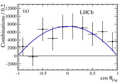
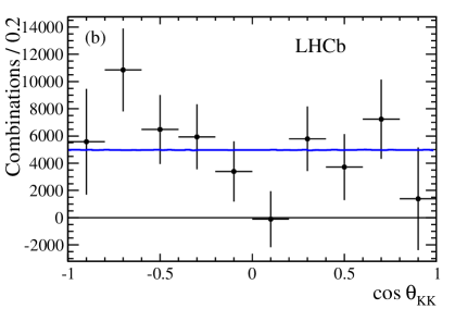
Figure 16: Background-subtracted and efficiency-corrected distribution of (a) $\cos\theta_{{J\mskip-3.0mu/\mskip-2.0mu\psi\mskip 2.0mu}}$ ($\chi^{2}/\rm ndf=5.3/10$) and (b) $\cos\theta_{KK}$ ($\chi^{2}/\rm ndf=12.8/10$). The points with error bars are data and the (blue) solid lines show the fit to the default model.

The background-subtracted and efficiency-corrected distributions of $\cos\theta_{{J\mskip-3.0mu/\mskip-2.0mu\psi\mskip 2.0mu}}$ and $\cos\theta_{KK}$ are shown in Fig. 16. Since all the contributing components are S-waves, the data should be distributed as $1-\cos^{2}\theta_{{J\mskip-3.0mu/\mskip-2.0mu\psi\mskip 2.0mu}}$ in $\cos\theta_{{J\mskip-3.0mu/\mskip-2.0mu\psi\mskip 2.0mu}}$ and uniformly in $\cos\theta_{KK}$. The $\cos\theta_{{J\mskip-3.0mu/\mskip-2.0mu\psi\mskip 2.0mu}}$ distribution follows the expectation very well with $\chi^{2}/\rm ndf=5.3/10$ and the $\cos\theta_{KK}$ is consistent with the uniform distribution with $\chi^{2}/\rm ndf=12.8/10$, corresponding to the spin-0 hypothesis for the $K^{+}\kern-1.60004ptK^{-}$ system in the ${J\mskip-3.0mu/\mskip-2.0mu\psi\mskip 2.0mu}K^{+}\kern-1.60004ptK^{-}$ final state.

4.5 Search for the $\kern 1.79993pt\overline{\kern-1.79993ptB}{}^{0}\rightarrow{J\mskip-3.0mu/\mskip-2.0mu\psi\mskip 2.0mu}\phi$ decay

The branching fraction of $\kern 1.79993pt\overline{\kern-1.79993ptB}{}^{0}\rightarrow{J\mskip-3.0mu/\mskip-2.0mu\psi\mskip 2.0mu}\phi$ is expected to be significantly suppressed, as the decay process $\kern 1.79993pt\overline{\kern-1.79993ptB}{}^{0}\rightarrow{J\mskip-3.0mu/\mskip-2.0mu\psi\mskip 2.0mu}\phi$ involves hadronic final state interactions at leading order. Here we search for the process by adding the $\phi$ resonance to the default Dalitz model. A Breit-Wigner function is used to model the $\phi$ lineshape with mass $1019.455\pm 0.020$ $\mathrm{\,Me\kern-1.00006ptV}$ and width $4.26\pm 0.04$ $\mathrm{\,Me\kern-1.00006ptV}$ [17]. The mass resolution is $\approx 0.7$ MeV at the $\phi$ mass peak, which is added to the fit model by increasing the Breit-Wigner width of the $\phi$ to 4.59 MeV. We do not find any evidence for the $\phi$ resonance. The best fit value for the $\phi$ fraction, constrained to be non-negative, is 0%. The corresponding upper limit at 90% CL is determined by generating 2000 experiments from the results of the fit with the $\phi$ resonance, where the correlations of the fitted parameters are also taken into account. The 90% CL upper limit on the $\phi$ fraction, defined as the fraction value that exceeds the results observed in 90% of the experiments, is 3.3%. The branching fraction upper limit is then the product of the fit fraction upper limit and the total branching fraction for $\kern 1.79993pt\overline{\kern-1.79993ptB}{}^{0}\rightarrow{J\mskip-3.0mu/\mskip-2.0mu\psi\mskip 2.0mu}K^{+}\kern-1.60004ptK^{-}$.

5 Branching fractions

Branching fractions are measured using the $B^{-}\rightarrow{J\mskip-3.0mu/\mskip-2.0mu\psi\mskip 2.0mu}K^{-}$ decay mode as normalization. This decay mode, in addition to having a well-measured branching fraction, has the advantage of having two muons in the final state and being collected through the same triggers as the $\kern 1.79993pt\overline{\kern-1.79993ptB}{}^{0}$ decays. The branching fractions are calculated using

$$\mathcal{B}(\kern 1.79993pt\overline{\kern-1.79993ptB}{}^{0}\rightarrow{J\mskip-3.0mu/\mskip-2.0mu\psi\mskip 2.0mu}K^{+}\kern-1.60004ptK^{-})=\frac{N_{\kern 1.25995pt\overline{\kern-1.25995ptB}{}^{0}}/\epsilon_{\kern 1.25995pt\overline{\kern-1.25995ptB}{}^{0}}}{N_{B^{-}}/\epsilon_{B^{-}}}\times\mathcal{B}(B^{-}\rightarrow{J\mskip-3.0mu/\mskip-2.0mu\psi\mskip 2.0mu}K^{-}),$$ (20)

where $N$ represents the observed yield of the decay of interest and $\epsilon$ corresponds to the overall efficiency. We form an average of $\mathcal{B}(B^{-}\rightarrow{J\mskip-3.0mu/\mskip-2.0mu\psi\mskip 2.0mu}K^{-})=(10.18\pm 0.42)\times 10^{-4}$ using the Belle  [25] and BaBar [26] measurements, corrected to take into account different rates of $B^{+}B^{-}$ and $B^{0}\kern 1.79993pt\overline{\kern-1.79993ptB}{}^{0}$ pair production from $\Upsilon(4S)$ using $\frac{\Gamma(B^{+}B^{-})}{\Gamma(B^{0}\kern 1.25995pt\overline{\kern-1.25995ptB}{}^{0})}=1.055\pm 0.025$ [17].

The detection efficiency is obtained from simulations and is a product of the geometrical acceptance of the detector, the combined reconstruction and selection efficiency and the trigger efficiency. Since the efficiency to detect the ${J\mskip-3.0mu/\mskip-2.0mu\psi\mskip 2.0mu}K^{+}\kern-1.60004ptK^{-}$ final state is not uniform across the Dalitz plane, the efficiency is averaged according to the default Dalitz model. Small corrections are applied to account for differences between the simulation and the data. To ensure that the $p$ and $p_{\rm T}$ distributions of the generated $B$ meson are correct we weight the simulated samples to match the distributions of the corresponding data. Since the normalization channel has a different number of charged tracks than the signal channel, we weight the simulated samples with the tracking efficiency ratio by comparing the data and simulations in the track’s $p$ and $p_{\rm T}$ bins. Finally, we weight the simulations according to the kaon identification efficiency. The average of the weights is assigned as a correction factor. Multiplying the detection efficiencies and correction factors gives the overall efficiencies $(0.820\pm 0.012)\%$ and $(2.782\pm 0.047)\%$ for $\kern 1.79993pt\overline{\kern-1.79993ptB}{}^{0}\rightarrow{J\mskip-3.0mu/\mskip-2.0mu\psi\mskip 2.0mu}K^{+}\kern-1.60004ptK^{-}$ and $B^{-}\rightarrow{J\mskip-3.0mu/\mskip-2.0mu\psi\mskip 2.0mu}K^{-}$, respectively.

The resulting branching fraction is

$$\mathcal{B}(\kern 1.79993pt\overline{\kern-1.79993ptB}{}^{0}\rightarrow{J\mskip-3.0mu/\mskip-2.0mu\psi\mskip 2.0mu}K^{+}K^{-})=(2.53\pm 0.31\pm 0.19)\times 10^{-6},$$

where the first uncertainty is statistical and the second is systematic. The systematic uncertainties are discussed in Section 6. This branching fraction has not been measured previously.

The product branching fraction of the $a_{0}(980)$ resonance mode is measured for the first time, yielding

$$\mathcal{B}(\kern 1.79993pt\overline{\kern-1.79993ptB}{}^{0}\rightarrow{J\mskip-3.0mu/\mskip-2.0mu\psi\mskip 2.0mu}a_{0}(980),~{}a_{0}(980)\rightarrow K^{+}\kern-1.60004ptK^{-})=(4.70\pm 3.31\pm 0.72)\times 10^{-7},$$

calculated by multiplying the corresponding fit fraction from the default model and the total branching fraction of the $\kern 1.79993pt\overline{\kern-1.79993ptB}{}^{0}\rightarrow{J\mskip-3.0mu/\mskip-2.0mu\psi\mskip 2.0mu}K^{+}\kern-1.60004ptK^{-}$ decay. The difference between the default and alternate model is assigned as a systematic uncertainty. The $a_{0}(980)$ resonance has a statistical significance of 3.9 standard deviations, showing evidence of the existence of $\kern 1.79993pt\overline{\kern-1.79993ptB}{}^{0}\rightarrow{J\mskip-3.0mu/\mskip-2.0mu\psi\mskip 2.0mu}a_{0}(980)$ with $a_{0}(980)\rightarrow K^{+}\kern-1.60004ptK^{-}$. Since the significance is less than five standard deviations, we also quote an upper limit on the branching fraction,

$$\mathcal{B}(\kern 1.79993pt\overline{\kern-1.79993ptB}{}^{0}\rightarrow{J\mskip-3.0mu/\mskip-2.0mu\psi\mskip 2.0mu}a_{0}(980),~{}a_{0}(980)\rightarrow K^{+}\kern-1.60004ptK^{-})<9.0\times 10^{-7}$$

at 90% CL. The limit is calculated assuming a Gaussian distribution as the central value plus 1.28 times the statistical and systematic uncertainties added in quadrature.

The upper limit of $\mathcal{B}(\kern 1.79993pt\overline{\kern-1.79993ptB}{}^{0}\rightarrow{J\mskip-3.0mu/\mskip-2.0mu\psi\mskip 2.0mu}\phi)$ is determined to be

$$\mathcal{B}(\kern 1.79993pt\overline{\kern-1.79993ptB}{}^{0}\rightarrow{J\mskip-3.0mu/\mskip-2.0mu\psi\mskip 2.0mu}\phi)<1.9\times 10^{-7}$$

at 90% CL, where the branching fraction $\mathcal{B}(\phi\rightarrow K^{+}\kern-1.60004ptK^{-})=(48.9\pm 0.5)\%$ is used and the systematic uncertainties on the branching fraction of $\kern 1.79993pt\overline{\kern-1.79993ptB}{}^{0}\rightarrow{J\mskip-3.0mu/\mskip-2.0mu\psi\mskip 2.0mu}K^{+}\kern-1.60004ptK^{-}$ are included. The limit improves upon the previous best limit of $<9.4\times 10^{-7}$ at 90% CL, given by the Belle collaboration [27]. According to a theoretical calculation based on $\omega-\phi$ mixing (see Appendix A) the branching fraction of $\kern 1.79993pt\overline{\kern-1.79993ptB}{}^{0}\rightarrow{J\mskip-3.0mu/\mskip-2.0mu\psi\mskip 2.0mu}\phi$ is expected to be $(1.0\pm 0.3)\times 10^{-7}$, which is consistent with our limit.

6 Systematic uncertainties

The systematic uncertainties on the branching fractions are estimated from the contributions listed in Table 2. Since the branching fractions are measured with respect to the $B^{-}\rightarrow{J\mskip-3.0mu/\mskip-2.0mu\psi\mskip 2.0mu}K^{-}$ mode, which has a different number of charged tracks than the decays of interest, a 1% systematic uncertainty is assigned due to differences in the tracking performance between data and simulation. A 2% uncertainty is assigned for the decay in flight, large multiple scatterings and hadronic interactions of the additional kaon.

Table 2: Relative systematic uncertainties on branching fractions (%).

Source of uncertainty	${J\mskip-3.0mu/\mskip-2.0mu\psi\mskip 2.0mu}K^{+}K^{-}$	${J\mskip-3.0mu/\mskip-2.0mu\psi\mskip 2.0mu}a_{0}(980)$
Tracking efficiency	1.0	1.0
Material and physical effects	2.0	2.0
PID efficiency	1.0	1.0
$\kern 1.79993pt\overline{\kern-1.79993ptB}{}^{0}$ $p$ and $p_{\rm T}$ distributions	0.5	0.5
$B^{-}$ $p$ and $p_{\rm T}$ distributions	0.5	0.5
Simulation sample size	0.6	0.6
Background modeling	5.7	5.7
$\mathcal{B}(B^{-}\rightarrow{J\mskip-3.0mu/\mskip-2.0mu\psi\mskip 2.0mu}K^{-})$	4.1	4.1
Alternate model	-	13.4
Total	7.5	15.4

Small uncertainties are introduced if the simulation does not have the correct $B$ meson kinematic distributions. The measurement is relatively insensitive to any of these differences in the $B$ meson $p$ and $p_{\rm T}$ distributions since we are measuring the relative rates. By varying the $p$ and $p_{\rm T}$ distributions we see a maximum difference of 0.5%. There is a 1% systematic uncertainty assigned for the relative particle identification efficiencies. We find a 5.7% difference in the $\kern 1.79993pt\overline{\kern-1.79993ptB}{}^{0}$ signal yield when the shape of the combinatorial background is changed from a linear to a parabolic function. In addition, the difference of the $a_{0}(980)$ fraction between the default and alternate fit models is assigned as a systematic uncertainty for the $\mathcal{B}(\kern 1.79993pt\overline{\kern-1.79993ptB}{}^{0}\rightarrow{J\mskip-3.0mu/\mskip-2.0mu\psi\mskip 2.0mu}a_{0}(980),~{}a_{0}(980)\rightarrow K^{+}\kern-1.60004ptK^{-})$ upper limit. The total systematic uncertainty is obtained by adding each source of systematic uncertainty in quadrature as they are assumed to be uncorrelated.

7 Conclusions

We report the first observation of the $\kern 1.79993pt\overline{\kern-1.79993ptB}{}^{0}\rightarrow{J\mskip-3.0mu/\mskip-2.0mu\psi\mskip 2.0mu}K^{+}\kern-1.60004ptK^{-}$ decay. The branching fraction is determined to be

$$\mathcal{B}(\kern 1.79993pt\overline{\kern-1.79993ptB}{}^{0}\rightarrow{J\mskip-3.0mu/\mskip-2.0mu\psi\mskip 2.0mu}K^{+}K^{-})=(2.53\pm 0.31\pm 0.19)\times 10^{-6},$$

where the first uncertainty is statistical and the second is systematic. The resonant structure of the decay is studied using a modified Dalitz plot analysis where we include the helicity angle of the ${J\mskip-3.0mu/\mskip-2.0mu\psi\mskip 2.0mu}$. The decay is dominated by an S-wave in the $K^{+}\kern-1.60004ptK^{-}$ system. The product branching fraction of the $a_{0}(980)$ resonance mode is measured to be

$$\mathcal{B}(\kern 1.79993pt\overline{\kern-1.79993ptB}{}^{0}\rightarrow{J\mskip-3.0mu/\mskip-2.0mu\psi\mskip 2.0mu}a_{0}(980),~{}a_{0}(980)\rightarrow K^{+}\kern-1.60004ptK^{-})=(4.70\pm 3.31\pm 0.72)\times 10^{-7},$$

which corresponds to a 90% CL upper limit of $\mathcal{B}(\kern 1.79993pt\overline{\kern-1.79993ptB}{}^{0}\rightarrow{J\mskip-3.0mu/\mskip-2.0mu\psi\mskip 2.0mu}a_{0}(980),~{}a_{0}(980)\rightarrow K^{+}\kern-1.60004ptK^{-})<9.0\times 10^{-7}$. We also set an upper limit of $\mathcal{B}(\kern 1.79993pt\overline{\kern-1.79993ptB}{}^{0}\rightarrow{J\mskip-3.0mu/\mskip-2.0mu\psi\mskip 2.0mu}\phi)<1.9\times 10^{-7}$ at the 90% CL. This result represents an improvement of about a factor of five with respect to the previous best measurement [27].

Appendix

Appendix A $\omega-\phi$ mixing

In Ref. [4], Gronau and Rosner pointed out that the decay $\kern 1.79993pt\overline{\kern-1.79993ptB}{}^{0}\rightarrow{J\mskip-3.0mu/\mskip-2.0mu\psi\mskip 2.0mu}\phi$ can proceed via $\omega-\phi$ mixing and predicted ${\cal{B}}(\kern 1.79993pt\overline{\kern-1.79993ptB}{}^{0}\rightarrow{J\mskip-3.0mu/\mskip-2.0mu\psi\mskip 2.0mu}\phi)=(1.8\pm 0.3)\times 10^{-7}$, using ${\cal{B}}(\kern 1.79993pt\overline{\kern-1.79993ptB}{}^{0}\rightarrow{J\mskip-3.0mu/\mskip-2.0mu\psi\mskip 2.0mu}\rho)=(2.7\pm 0.4)\times 10^{-5}$ [17] as there was no measurement of ${\cal{B}}(\kern 1.79993pt\overline{\kern-1.79993ptB}{}^{0}\rightarrow{J\mskip-3.0mu/\mskip-2.0mu\psi\mskip 2.0mu}\omega)$ available. Recently LHCb has measured ${\cal{B}}(\kern 1.79993pt\overline{\kern-1.79993ptB}{}^{0}\rightarrow{J\mskip-3.0mu/\mskip-2.0mu\psi\mskip 2.0mu}\omega)=(2.41\pm 0.52\,^{+0.41}_{-0.50})\times 10^{-5}$ [28], which can be used to update the prediction.

The mixing $\omega-\phi$ is parametrized by a $2\times 2$ rotation matrix characterized by the angle $\delta_{m}$ such that the physical $\omega$ and $\phi$ are related to the ideally mixed states $\omega^{I}\equiv\frac{1}{\sqrt{2}}(u\overline{}u+d\overline{}d)$ and $\phi^{I}\equiv s\overline{}s$, giving

$$\omega = \;\;\;\cos\delta_{m}\omega^{I}+\sin\delta_{m}\phi^{I}$$

$$\phi = -\sin\delta_{m}\omega^{I}+\cos\delta_{m}\phi^{I}.$$ (21)

This implies

$${\cal{B}}(\kern 1.79993pt\overline{\kern-1.79993ptB}{}^{0}\rightarrow{J\mskip-3.0mu/\mskip-2.0mu\psi\mskip 2.0mu}\phi)=\tan^{2}\delta_{m}{\cal{B}}(\kern 1.79993pt\overline{\kern-1.79993ptB}{}^{0}\rightarrow{J\mskip-3.0mu/\mskip-2.0mu\psi\mskip 2.0mu}\omega)\Phi,$$ (22)

where $\Phi$ represents the ratio of phase spaces between the processes $\kern 1.79993pt\overline{\kern-1.79993ptB}{}^{0}\rightarrow{J\mskip-3.0mu/\mskip-2.0mu\psi\mskip 2.0mu}\phi$ and $\kern 1.79993pt\overline{\kern-1.79993ptB}{}^{0}\rightarrow{J\mskip-3.0mu/\mskip-2.0mu\psi\mskip 2.0mu}\omega$.

A simplified analysis [29] implies a mixing angle of $\delta_{m}=(3.34\pm 0.17)^{\circ}$, while allowing an energy dependent $\delta_{m}$ gives values of $2.75^{\circ}$ at the $\omega$ mass and $3.84^{\circ}$ at the $\phi$ mass [30]. Using the recent LHCb value of ${\cal{B}}(\kern 1.79993pt\overline{\kern-1.79993ptB}{}^{0}\rightarrow{J\mskip-3.0mu/\mskip-2.0mu\psi\mskip 2.0mu}\omega)$ and $3.84^{\circ}$ for $\delta_{m}$, we estimate the following value

$${\cal{B}}(\kern 1.79993pt\overline{\kern-1.79993ptB}{}^{0}\rightarrow{J\mskip-3.0mu/\mskip-2.0mu\psi\mskip 2.0mu}\phi)=(1.0\pm 0.3)\times 10^{-7}.$$ (23)

References

- [1] LHCb collaboration, R. Aaij et al., Analysis of the resonant components in , Phys. Rev. D86 (2012) 052006, arXiv:1204.5643
- [2] LHCb collaboration, R. Aaij et al., Amplitude analysis and branching fraction measurement of , Phys. Rev. D87 (2013) 072004, arXiv:1302.1213
- [3] LHCb collaboration, R. Aaij et al., Analysis of the resonant components in , Phys. Rev. D87 (2013) 052001, arXiv:1301.5347
- [4] M. Gronau and J. L. Rosner, decays dominated by mixing, Phys. Lett. B666 (2008) 185, arXiv:0806.3584
- [5] R. H. Dalitz, On the analysis of -meson data and the nature of the -meson, Philosophical Magazine 44 (1953) 1068
- [6] LHCb collaboration, A. A. Alves Jr. et al., The LHCb detector at the LHC, JINST 3 (2008) S08005
- [7] M. Adinolfi et al., Performance of the LHCb RICH detector at the LHC, Eur. Phys. J. C73 (2013) 2431, arXiv:1211.6759
- [8] A. A. Alves, Jr. et al., Performance of the LHCb muon system, JINST 8 (2013) P02022, arXiv:1211.1346
- [9] R. Aaij et al., The LHCb trigger and its performance in 2011, JINST 8 (2013) P04022, arXiv:1211.3055
- [10] T. Sjöstrand, S. Mrenna, and P. Skands, PYTHIA 6.4 physics and manual, JHEP 0605 (2006) 026, arXiv:hep-ph/0603175
- [11] I. Belyaev et al., Handling of the generation of primary events in Gauss, the LHCb simulation framework, Nuclear Science Symposium Conference Record (NSS/MIC) IEEE (2010) 1155
- [12] D. J. Lange, The EvtGen particle decay simulation package, Nucl. Instrum. Meth. A462 (2001) 152
- [13] P. Golonka and Z. Was, Photos Monte Carlo: a precision tool for QED corrections in and decays, Eur. Phys. J. C45 (2006) 97, arXiv:hep-ph/0506026
- [14] Geant4 collaboration, J. Allison et al., Geant4 developments and applications, IEEE Trans. Nucl. Sci. 53 (2006) 270
- [15] Geant4 collaboration, S. Agostinelli et al., GEANT4: A simulation toolkit, Nucl. Instrum. Meth. A506 (2003) 250
- [16] M. Clemencic et al., The LHCb simulation application, Gauss: design, evolution and experience, J. Phys. Conf. Ser. 331 (2011), no. 3 032023
- [17] Particle Data Group, J. Beringer et al., Review of Particle Physics , Phys. Rev. D86 (2012) 010001
- [18] L. Breiman, J. H. Friedman, R. A. Olshen, and C. J. Stone, Classification and regression trees. Wadsworth international group, Belmont, California, USA, 1984
- [19] LHCb collaboration, R. Aaij et al., Precision measurement of the baryon lifetime, arXiv:1307.2476, to appear in PRL
- [20] BES collaboration, M. Ablikim et al., Partial wave analysis of , Phys. Rev. D72 (2005) 092002, arXiv:hep-ex/0508050
- [21] BaBar collaboration, B. Aubert et al., Dalitz plot analysis of the decay , Phys. Rev. D74 (2006) 032003, arXiv:hep-ex/0605003
- [22] S. M. Flatté, On the nature of mesons, Phys. Lett. B63 (1976) 228
- [23] A. Abele et al., annihilation at rest into , Phys. Rev. D57 (1998) 3860
- [24] S. Baker and R. D. Cousins, Clarification of the use of and likelihood functions in fits to histograms, Nucl. Instrum. Meth. 221 (1984) 437
- [25] Belle collaboration, K. Abe et al., Measurement of branching fractions and charge asymmetries for two-body B meson decays with charmonium, Phys. Rev. D67 (2003) 032003, arXiv:hep-ex/0211047
- [26] BaBar collaboration, B. Aubert et al., Measurement of branching fractions and charge asymmetries for exclusive decays to charmonium, Phys. Rev. Lett. 94 (2005) 141801, arXiv:hep-ex/0412062
- [27] Belle collaboration, Y. Liu et al., Search for decays, Phys. Rev. D78 (2008) 011106, arXiv:0805.3225
- [28] LHCb collaboration, R. Aaij et al., Evidence for the decay and measurement of the relative branching fractions of meson decays to and , Nucl. Phys. B 867 (2013) 547, arXiv:1210.2631
- [29] M. Benayoun, L. DelBuono, S. Eidelman, V. Ivanchenko, and H. B. O’Connell, Radiative decays, nonet symmetry and SU(3) breaking, Phys. Rev. D59 (1999) 114027, arXiv:hep-ph/9902326
- [30] M. Benayoun, P. David, L. DelBuono, and O. Leitner, A global treatment of VMD physics up to the : I. annihilations, anomalies and vector meson partial widths, Eur. Phys. J. C65 (2010) 211, arXiv:0907.4047