Fast dynamos in spherical boundary-driven flows

Abstract

We numerically demonstrate the feasibility of kinematic fast dynamos for a class of time-periodic axisymmetric flows of conducting fluid confined inside a sphere. The novelty of our work is in considering the realistic flows, which are self-consistently determined from the Navier-Stokes equation with specified boundary driving. Such flows can be achieved in a new plasma experiment, whose spherical boundary is capable of differential driving of plasma flows in the azimuthal direction. We show that magnetic fields are self-excited over a range of flow parameters such as amplitude and frequency of flow oscillations, fluid Reynolds ($Re$) and magnetic Reynolds ($Rm$) numbers. In the limit of large $Rm$, the growth rates of the excited magnetic fields are of the order of the advective time scales and practically independent of $Rm$, which is an indication of the fast dynamo.

It is now widely accepted that the observed magnetic fields of various astrophysical systems are due to the dynamo mechanism associated with the flows of highly conducting fluids in their interiors Moffatt_1978 ; Rudiger_2004 . In most of these systems the dynamos appear to be fast, i.e., they act on the fast advective time scales of the underlying flows, rather than on the slow resistive or intermediate time scales Vainshtein_1972 . The astrophysical relevance of fast dynamos stimulated intensive theoretical and numerical studies (Refs. Childress_1995 ; Galloway_2003 and references therein), however, they have never been studied experimentally. In this work we present a numerical analysis of fast dynamos in a class of spherical boundary-driven flows that can be obtained in a real plasma experiment.

Several conditions are required for a fast dynamo action. First, the fast dynamos only operate at high values of magnetic Reynolds number $Rm$ (usually, $Rm\gtrsim 10^{3}$), which is the ratio of the resistive and advective time scales. Second, the flow must be chaotic in order to yield a fast dynamo Finn_1988 ; Klapper_1995 . Both these conditions are satisfied in astrophysical flows, most of which are turbulent with extremely high $Rm$. Achieving flows with high $Rm$ is a major obstacle for experimental demonstration of fast dynamos, since this requires a highly conducting, quickly flowing fluid (for reference, the maximum value of $Rm$ in existing liquid metal experiments is $Rm\sim 10^{2}$).

Models with prescribed flows exhibiting fast dynamos in the kinematic (linear) stage have been considered in the literature for plane-periodic Galloway_1992 ; Hughes_1996 ; Dorch_2000 ; Tobias_2008 and spherical shell Hollerbach_1995 ; Hollerbach_1998 ; Livermore_2007 ; Richardson_2012 geometries. The common feature of the dynamo fields emerging in these models is that at high $Rm$ their structure is dominated by the rapidly varying small-scale fluctuations. The relationship between the small-scale dynamo and large-scale generation of flux is perhaps the most perplexing issue in dynamo theory. As shown recently in Refs. Hughes_2009 ; Tobias_2013 , an organized large-scale magnetic field can be produced in dynamo simulations if a global shear is also included into a helical plane-periodic flow.

More realistic models of dynamos include flows which are self-consistently determined from the Navier-Stokes equation with the appropriate forcing terms Brummel_1998 ; Cameron_2006 ; Livermore_2010 . In this case, the properties of fast dynamos (in both the linear and nonlinear stages) strongly depend on the magnetic Prandtl number $Pm=\nu/\eta$, the ratio of kinematic viscosity $\nu$ to resistivity $\eta$ of the medium. In astrophysical applications of fast dynamo theory two different limits are recognized: $Pm\ll 1$ (solar convective zone, protoplanetary accretion disks) and $Pm\gg 1$ (solar corona, interstellar medium, galaxies and galaxy clusters). In the former limit, the fluid is essentially inviscid on all magnetic scales, and the resulting dynamo is induced by the “rough” (highly fluctuating) velocity field Tobias_2012 ; Schekochihin_2007 . In the latter limit, the small velocity scales are dissipated more efficiently than the small magnetic scales, and the dynamo develops on the “smooth” (large scale) velocity field Tobias_2012 ; Schekochihin_2004 . The latter circumstance is important in our study: the case of $Pm\ll 1$ cannot be addressed without extensive numerical simulations of MHD turbulence, but the case of $Pm\gg 1$ can be modeled by a simple laminar, yet chaotic flow producing a fast dynamo structure.

Our present study is motivated by the successful initial operation of the Madison plasma dynamo experiment (MPDX), which is designed to investigate dynamos in controllable flows of hot, unmagnetized plasmas Spence_2009 . In the MPDX, plasma is confined inside a 3 m spherical vessel by an edge-localized multicusp magnetic field. A unique mechanism for driving plasma flows in the MPDX allows an arbitrary azimuthal velocity to be imposed along the boundary Collins_2012 . The most advantageous property of plasma is the ability to vary its characteristics by adjusting experimental controls. Indeed, the confinement properties of this device indicate that the low density, high temperature plasmas can be obtained with values of $Rm\sim 10^{4}$ and $Pm\sim 10^{2}$ required for a fast dynamo in a laminar flow.

The scope of our study is to numerically demonstrate kinematic fast dynamos for a class of time-periodic, boundary-driven, axisymmetric flows found self-consistently from the Navier-Stokes equation. In a sense, these flows are an adaptation of the plane-periodic Galloway-Proctor flow Galloway_1992 to the geometry of a full sphere with a viable driving force. Several models of flows resulting in fast dynamos have been considered in the spherical shells Hollerbach_1995 ; Hollerbach_1998 ; Livermore_2007 ; Richardson_2012 ; Livermore_2010 , but analogous studies for a full sphere are lacking. Furthermore, in all previous studies the flows are either prescribed or driven by artificial forces, so they are non physical and not reproducible in a real experiment. The class of flows considered in our study is more practical, since it can be realized in the MPDX by applying the corresponding plasma driving at the edge.

As a framework, we use incompressible magnetohydrodynamics (MHD), whose dimensionless equations are

$$\frac{\partial\textbf{v}}{\partial t} = \frac{1}{Re}\nabla^{2}\textbf{v}-(\textbf{v}\cdot\nabla)\textbf{v}-\nabla p,$$ (1)

$$\frac{\partial\tilde{\textbf{v}}}{\partial t} = \frac{1}{Re}\nabla^{2}\tilde{\textbf{v}}-(\tilde{\textbf{v}}\cdot\nabla)\textbf{v}-(\textbf{v}\cdot\nabla)\tilde{\textbf{v}}-\nabla\tilde{p},$$ (2)

$$\frac{\partial\textbf{B}}{\partial t} = \frac{1}{Rm}\nabla^{2}\textbf{B}+\nabla\times(\textbf{v}\times\textbf{B}),$$ (3)

$$0 = \nabla\cdot\textbf{v}=\nabla\cdot\tilde{\textbf{v}}=\nabla\cdot\textbf{B}.$$ (4)

Normalized quantities are defined using the radius of the sphere $R_{0}$ as a unit of length, the typical driving velocity at the edge $V_{0}$ as a unit of velocity, the turnover time $R_{0}/V_{0}$ as a unit of time, the plasma mass density $\rho_{0}$, the kinematic viscosity $\nu$ and the magnetic diffusivity $\eta$ (all three assumed to be constant and uniform). Normalization of the magnetic field B is arbitrary since it enters Eq. (3) linearly. The fluid Reynolds number $Re$ and the magnetic Reynolds number $Rm$ are introduced as $Re=R_{0}V_{0}/\nu$, $Rm=R_{0}V_{0}/\eta$, and their ratio determines magnetic Prandtl number $Pm=Rm/Re$. In this study we consider flows in a range of $Re=100-500$, $Rm=10^{3}-10^{5}$ and $Pm=2-500$, which overlaps with MPDX operating regimes. In these regimes, MPDX plasma is expected to have relatively small Mach numbers $M=V_{0}/C_{s}\approx 0.1-0.3$, where $C_{s}$ is the ion sound speed. This justifies the use of the incompressible model.

Eqs. (1)-(3) require appropriate boundary conditions. Eq. (1) is the Navier-Stokes equation and we use it to find equilibrium flows v. Since we are interested in the kinematic stage of a dynamo, we do not include the Lorentz force from the dynamo field in Eq. (1). We consider only axisymmetric, time-periodic equilibrium flows driven by the following boundary condition (Fig. 1):

$$\textbf{v}\big{|}_{r=1}=(\sin 2\theta+a\sin\theta\,\cos\omega t)\textbf{e}_{\phi},~{}~{}~{}0\leq\theta\leq\pi,$$ (5)

in a spherical system of coordinates $(r,\theta,\phi)$. As shown below, for some values of oscillation amplitude $a$ and frequency $\omega$ the corresponding equilibrium flows are hydrodynamically stable and can lead to fast dynamos. Eq. (2) is the linearized Navier-Stokes equation for the flow perturbations $\tilde{\textbf{v}}$. It is used to establish the hydrodynamic stability properties of the equilibrium flows v. Assuming impenetrable, no-slip wall, we have $\tilde{\textbf{v}}\big{|}_{r=1}=0$. Eq. (3) is the kinematic dynamo problem with a velocity field v satisfying Eqs. (1), (5). The choice of magnetic boundary conditions can strongly affect the dynamo action Khalzov_2012b . In our present study we assume the non-ferritic, perfectly conducting wall, coated inside with a thin insulating layer. This model reflects the actual boundary in the MPDX. Corresponding conditions for B are $B_{r}\big{|}_{r=1}=(\nabla\times\textbf{B})_{r}\big{|}_{r=1}=0$, i.e., normal components of both magnetic field and current are zero at the boundary.

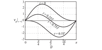
Figure 1: Time-periodic boundary-driving azimuthal velocity $v_{\phi}$ from Eq. (5) with oscillation amplitude $a=2$ as a function of polar angle $\theta$ at several moments over a period $T=2\pi/\omega$.

We briefly describe the numerical methods used for solving Eqs. (1)-(3). The divergence-free fields v, $\tilde{\textbf{v}}$ and B are expanded in a spherical harmonic basis Bullard_1954 (the resulting equations can be found, for example, in Ref. Khalzov_2012c ). The radial discretization of these equations is based on a Galerkin scheme with Chebyshev polynomials Livermore_2005 . This discretization provides fast convergence: truncation at $N_{p}=100$ spherical harmonics and $N_{r}=100$ radial polynomials gives 4 converged significant digits in the dynamo growth rate for $Rm=50\,000$. To solve the discretized Eq. (1) for a time-periodic equilibrium velocity v we apply a Fourier time transform to v and use the iterative scheme analogous to the one from Ref. Khalzov_2012c . Since the equilibrium velocity is axisymmetric, modes with different azimuthal numbers $m$ are decoupled in Eqs. (2), (3). For a time-periodic flow v, these equations constitute the standard Floquet eigenvalue problems Kuchment_1993 . Eq. (3) has a solution of the form $\textbf{B}(\textbf{r},t)=e^{\gamma t}\tilde{\textbf{B}}(\textbf{r},t)$, where $\gamma$ is the complex eigenvalue (Floquet exponent) and $\tilde{\textbf{B}}(\textbf{r},t)$ is time-periodic with a period $T=2\pi/\omega$ of the flow (solution to Eq. (2) is analogous). We solve Eqs. (2), (3) in discretized form using the Arnoldi iteration method, which finds the eigenvalues with the largest real part (growth rate). More details on application of this method to a kinematic dynamo problem are given in Ref. Willis_2004 .

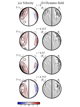
Figure 2: Structure of (a) equilibrium velocity v and (b) fastest dynamo eigenmode B (with azimuthal number $m=1$) at four consecutive moments over a period $T=2\pi/\omega$. The flow parameters are $a=2$, $\omega=0.6$, $Re=300$, $Rm=30\,000$, the respective dynamo eigenvalue is $\gamma=0.059627+0.200510i$. Exponential growth and rotation associated with $\gamma$ are removed from the images of B by a suitable normalization (the resulting B is periodic with period $T$). The left half of each figure shows the modulus of the poloidal (lying in meridional plane) component, the right half shows a level plot of the azimuthal component. In velocity figures, contours with arrows are stream lines of poloidal velocity $v_{pol}$, dashed curves denote levels of $v_{\phi}<0$. In dynamo figures, lighting is used to emphasize the small-scale structure of dynamo field. The listed parameters correspond to the MPDX fully ionized hydrogen plasma with the density $n_{0}\approx 2\cdot 10^{12}$ cm^-3, the ion temperature $T_{i}\approx 1$ eV, the electron temperature $T_{e}\approx 100$ eV, the typical driving velocity $V_{0}\approx 12.5$ km/s, the driving frequency $\omega/2\pi\approx 0.8$ kHz and the dynamo growth rate $\gamma_{r}\approx 500$ s^-1 (see Ref. Spence_2009 for details).

An example of the calculated equilibrium velocity is shown in Fig. 2(a). The flow is axisymmetric with well defined laminar structure at every instant of time. However, the paths of fluid elements in such flow are chaotic (Fig. 3). From a practical point of view, it is important to have a hydrodynamically stable flow, so the flow properties do not change over the course of experiment and the predicted fast dynamos can be obtained. We study the linear stability of the flows by solving Eq. (2). The stability boundaries in the parameter space of $(\omega,a,Re)$ are shown in Fig. 4. They are determined by non-axisymmetric modes only ($m=1-4$), the axisymmetric modes ($m=0$) are always stable for the considered flows. The stable region becomes smaller as fluid Reynolds number $Re$ increases. We note that the steady counter-rotating flow corresponding to the boundary drive with $a=0$ is linearly unstable when $Re>120$. The time-periodic dependence of the flow plays twofold role: first, it stabilizes the fluid motion, and second, it leads to the chaotic streamlines required for the fast dynamo mechanism. The former is analogous to parametric stabilization observed in Kapitza’s pendulum – an inverted pendulum with pivot point vibrating in vertical direction Kapitza_1951 .

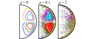
Figure 3: Poincaré plots for the equilibrium flow v for $Re=300$, $\omega=0.6$ and three amplitudes $a$. Points are the footprints of trajectories of six fluid parcels shown in different colors at one meridional plane. Each trajectory is followed for $1000T$.

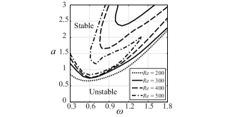
Figure 4: Hydrodynamic stability boundaries of the equilibrium flow v on the plane of driving parameters $(\omega,a)$ for different fluid Reynolds numbers $Re$. For every $Re$, curves are composed of several azimuthal modes $m$ (typically, $m=1-4$). The shown region of parameters is stable for $Re<120$.

Fig. 5 summarizes the results of our kinematic dynamo studies. The figure shows the dependences of the dynamo growth rate $\gamma_{r}$ (real part of the eigenvalue) on magnetic Reynolds number $Rm$ for different flow parameters. It is apparent that in most cases the dependences tend to level off with increasing $Rm$. Such asymptotic behavior is a signature of fast dynamo action. Although none of these cases reaches its asymptotic state completely, they still suggest that fast dynamos are excited in the system. We note that the growth rates do not saturate until $Rm\sim 10^{5}$, whereas in the Galloway-Proctor flow Galloway_1992 this occurs at $Rm\sim 10^{2}-10^{3}$. A possible explanation was proposed in Ref. Hollerbach_1995 : in the spherical geometry the azimuthal number $m$ is restricted to integer values only, but in the plane-periodic geometry the corresponding wave-number is continuous and can be optimized to yield the largest growth rate. This also may explain why the typical critical $Rm$ required for the dynamo onset in our model ($Rm_{cr}\sim 10^{3}$) is much higher than the one in the Galloway-Proctor flow ($Rm_{cr}\sim 1$). Note that the value of $Rm_{cr}\sim 10^{3}$ can be achieved in MPDX by producing plasma with the electron temperature $T_{e}\sim 10$ eV and the driving velocity $V_{0}\sim 10$ km/s.

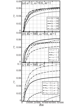
Figure 5: Dynamo growth rate $\gamma_{r}$ of the fastest mode as a function of $Rm$ for different values of (a) fluid Reynolds number $Re$, (b) oscillation amplitude $a$, (c) driving frequency $\omega$. Note that in (a) and (b) the fastest azimuthal modes are always $m=1$, while in (c) they vary with $\omega$.

The asymptotic values of the dynamo growth rates are determined by the flow properties. Most clearly this can be seen by changing driving frequency $\omega$ in Fig. 5(c). The largest value of $\gamma_{r}\approx 0.1$ (in units of inverse turnover time $V_{0}/R_{0}$) is achieved with the largest frequency $\omega=1.5$. Simulations show that for $\omega\gtrsim 1.7$ (at $Re=300,a=2$) the flow becomes hydrodynamically unstable, and our assumption of flow axisymmetry breaks. Another interesting point is that the fastest dynamo modes correspond to different azimuthal numbers $m$ ($m=1-3$) at different driving frequencies $\omega$. This is likely related to details of the equilibrium flow structure: as shown in Ref. Richardson_2012 , the optimum $m$ depends on the number of poloidal flow cells, which in our case varies with $\omega$.

The dynamo eigenmode is shown in Fig. 2(b). Due to our choice of the boundary conditions the magnetic field is fully contained inside the sphere. This is usually referred to as hidden dynamo, because it does not exhibit itself outside the bounded volume. The induced magnetic field has a fast-varying, small-scale structure. Such field is often characterized by the magnetic Taylor microscale, defined as the inverse of the effective wave-number $k_{eff}=(\langle|\nabla\times\textbf{B}|^{2}\rangle/\langle|\textbf{B}|^{2}\rangle)^{1/2}$, where $\langle\rangle$ denotes volume averaging. Fig. 6 shows that for large $Rm$ the scaling law for $k_{eff}$ is approaching $k_{eff}\sim Rm^{1/2}$. Similar scaling is also observed in some slow dynamos Perkins_1987 . The difference between the slow dynamo as in Ref. Perkins_1987 and the fast dynamo under consideration is that in the former case the magnetic structures with spatial scales of the order of $Rm^{-1/2}$ occur only in a small region near the separatrix of the flow, whereas in the latter case these structures are seen over a much larger region.

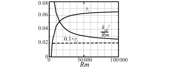
Figure 6: Square of the effective wave-number in a dynamo eigenmode $k_{eff}^{2}$ normalized by $Rm$ and corresponding dynamo eigenvalue $\gamma=\gamma_{r}+i\gamma_{i}$ as functions of $Rm$. Flow parameters are $Re=300$, $a=2$, $\omega=0.6$.

In conclusion, we numerically demonstrated the possibility of fast dynamo action in spherical boundary-driven time-periodic flows. This is an important step towards realizing the fast dynamos for the first time in plasma experiments such as MPDX.

The authors wish to thank S. Boldyrev, B. P. Brown, F. Cattaneo and E. Zweibel for valuable discussions. This work is supported by the NSF Award PHY 0821899 PFC Center for Magnetic Self Organization in Laboratory and Astrophysical Plasmas.

References

- (1) H. K. Moffatt, Magnetic Field Generation in Electrically Conducting Fluids (Cambridge University Press, Cambridge, 1978).
- (2) G. Rüdiger and R. Hollerbach, The Magnetic Universe: Geophysical and Astrophysical Dynamo Theory (Wiley-VCH, Weinheim, Germany, 2004).
- (3) S. I. Vainshtein and Ya. B. Zel’dovich, Sov. Phys. Usp. 15, 159 (1972).
- (4) S. Childress and A. D. Gilbert, Stretch, Twist, Fold: The Fast Dynamo (Springer-Verlag, Berlin, 1995).
- (5) D. J. Galloway, in Advances in Nonlinear Dynamos (Taylor & Francis, London, 2003), p. 37.
- (6) J. M. Finn and E. Ott, Phys. Fluids 31, 2992 (1988).
- (7) I. Klapper and L. S. Young, Commun. Math. Phys. 173, 623 (1995).
- (8) D. J. Galloway and M. R. E. Proctor, Nature 356, 691 (1992).
- (9) D. W. Hughes, F. Cattaneo, and E.-j. Kim, Phys. Lett. A 223, 167 (1996).
- (10) S. B. F. Dorch, Physica Scripta 61, 717 (2000).
- (11) S. M. Tobias and F. Cattaneo, J. Fluid Mech. 601, 101 (2008).
- (12) R. Hollerbach, D. J. Galloway, and M. R. E. Proctor, Phys. Rev. Lett. 74, 3145 (1995).
- (13) R. Hollerbach, D. J. Galloway, and M. R. E. Proctor, Geophys. Astrophys. Fluid Dynamics 87, 111 (1998).
- (14) P. W. Livermore, D. W. Hughes, and S. M. Tobias, Phys. Fluids 19, 057101 (2007).
- (15) K. J. Richardson, R. Hollerbach, and M. R. E. Proctor, Phys. Fluids 24, 107103 (2012).
- (16) D. W. Hughes and M. R. E. Proctor, Phys. Rev. Lett 102, 044501 (2009).
- (17) S. M. Tobias and F. Cattaneo, Nature 497, 463 (2013).
- (18) N. H. Brummel, F. Cattaneo, and S. M. Tobias, Phys. Lett. A 249, 437 (1998).
- (19) R. Cameron and D. J. Galloway, Mon. Not. R. Astron. Soc. 365, 735 (2006).
- (20) P. W. Livermore, D. W. Hughes, and S. M. Tobias, Phys. Fluids 22, 037101 (2010).
- (21) S. M. Tobias, F. Cattaneo, and S. Boldyrev, in Ten Chapters in Turbulence (Cambridge University Press, Cambridge, 2012), p. 351.
- (22) A. A. Schekochihin, A. B. Iskakov, S. C. Cowley, J. C. McWilliams, M. R. E. Proctor, and T. A. Yousef, New J. Phys. 9, 300 (2007).
- (23) A. A. Schekochihin, S. C. Cowley, S. F. Taylor, J. L. Maron, and J. C. McWilliams, Astrophys. J. 612, 276 (2004).
- (24) E. J. Spence, K. Reuter, and C. B. Forest, Astrophys. J. 700, 470 (2009).
- (25) C. Collins, N. Katz, J. Wallace, J. Jara-Almonte, I. Reese, E. Zweibel, and C. B. Forest, Phys. Rev. Lett. 108, 115001 (2012).
- (26) I. V. Khalzov, B. P. Brown, E. J. Kaplan, N. Katz, C. Paz-Soldan, K. Rahbarnia, E. J. Spence, and C. B. Forest, Phys. Plasmas 19, 104501 (2012).
- (27) E. C. Bullard, and H. Gellman, Phil. Trans. R. Soc. Lond. A 247, 213 (1954).
- (28) I. V. Khalzov, B. P. Brown, C. M. Cooper, D. B. Weisberg, and C. B. Forest, Phys. Plasmas 19, 112106 (2012).
- (29) P. W. Livermore, and A. Jackson, Geophys. Astrophys. Fluid Dynamics 99, 467 (2005).
- (30) P. A. Kuchment, Floquet Theory for Partial Differential Equations (Birkhäuser, 1993).
- (31) A. P. Willis and D. Gubbins, Geophys. Astrophys. Fluid Dynamics, 98, 537 (2004).
- (32) P. L. Kapitza, Sov. Phys. JETP, 21, 588 (1951).
- (33) F. W. Perkins and E. G. Zweibel, Phys. Fluids 30, 1079 (1987).