Dark energy imprints on the kinematic Sunyaev-Zel’dovich signal

Abstract

We investigate the imprint of dark energy on the kinetic Sunyaev-Zel’dovich (kSZ) angular power spectrum on scales of $\ell=1000$ to $10000$, and find that the kSZ signal is sensitive to the dark energy parameter. For example, varying the constant $w$ by 20% around $w=-1$ results in a $\gtrsim 10\%$ change on the kSZ spectrum; changing the dark energy dynamics parametrized by $w_{a}$ by $\pm 0.5$, a 30% change on the kSZ spectrum is expected. We discuss the observational aspects and develop a fitting formula for the kSZ power spectrum. Finally, we discuss how the precise modeling of the post-reionization signal would help the constraints on patchy reionization signal, which is crucial for measuring the duration of reionization.

I Introduction

Dark energy (DE), the energy source that drives our Universe accelerating, has remained a mystery since it was discovered in 1998 Riess et al. (1998); Perlmutter et al. (1999). The key feature of dark energy is encoded in its equation of state (hereafter EoS) parameter $w$, which is the ratio of its pressure to the energy density. The time dependence of EoS can be used to classify a range of DE models. The accumulating observational data, including observations of the cosmic microwave background radiation (CMB) Hinshaw et al. (2013); Planck results XVI. (2013), Type-Ia supernovae (SN) data Conley et al. (2011); Suzuki et al. (2012) and baryon acoustic oscillation (BAO) from galaxy surveys Beutler et al. (2011); Padmanabhan et al. (2012); Anderson et al. (2012); Blake et al. (2012) have set up strong constraints on the EoS of dark energy. Assuming the dark energy EoS is a constant, then recent observation from Wilkinson Microwave Anisotropy Probe (WMAP) gives the constraint $w=-1.073\pm 0.180$ ($95\%$ confidence level, WMAP9+extra CMB data +BAO+$H_{0}$, Hinshaw et al. (2013)), and observation from Planck satellite gives $w=-1.24^{+0.18}_{-0.19}$ ($95\%$ CL from Planck+$H_{0}$+WMAP polarization data, Planck results XVI. (2013)). However, allowing time evolution of $w$, the results of constraints become comparatively looser. For example, parameterizing dark energy EoS as $w(a)=w_{0}+w_{a}(1-a)$ then the constraints from WMAP9+extra CMB data +BAO+SN+$H_{0}$ is $w_{0}=-1.34\pm 0.36$ and $w_{a}=0.85\pm 0.94$ ($95\%$ CL, see table 10 of Hinshaw et al. (2013)), and from Planck+$H_{0}$+WMAP polarization data it is $w_{0}=-1.04^{+0.72}_{-0.69}$ and $w_{a}<1.32$ at ($95\%$ CL). Therefore, the data slightly favor the model with $w_{0}<-1$ and $w_{a}>0$ while large uncertainties of parameters still exist in the recent observational constraints.

In the spirit of exploring more phenomena associated with dark energy, we would like to investigate how the dark energy affects the growth of structure and clustering properties of galaxies. The kinematic Sunyaev-Zel’dovich (hereafter kSZ, or kinetic SZ) effect is one of the important phenomena that relates the galaxy’s peculiar motion with the temperature fluctuations of the CMB. The effect can arise during two processes, i.e. consisting of the “inhomogeneous patchy reionization” and the post-reionization signals.

In models of inhomogeneous reionization (or “patchy reionization”), where different regions of the Universe were ionized at different times, the bulk motion of bubbles of free electrons around the UV emitting sources may cause the temperature anisotropy on the CMB Gruzinov & Hu (1998); Fan, Carilli, & Keating (2006); Iliev et al. (2006); Knox, Scoccimarro & Dodelson (1998); McQuinn et al. (2005); Santos et al. (2003); Zahn et al. (2005, 2012). It has been demonstrated Zahn et al. (2005); McQuinn et al. (2005) that the magnitude of the kSZ power from patchy reionization is related to the duration of reionization. Hence, one can set a constraint on the duration of reionization ($\Delta z_{\rm rei}$) once the optical depth to reionization can be measured Zahn et al. (2012). After reionization, the “secondary anisotropy” of CMB can also be generated from the peculiar motion of galaxy clusters. Thus by measuring the kSZ effect one can have a good handle on the peculiar velocity of galaxies and therefore infer the growth rate of large scale structure. The growth rate of the large scale structure is affected by the dark energy EoS, because the dark energy negative pressure can drive the accelerated expansion of the Universe and therefore halt the growth of structure at late times. Therefore, it is necessary to investigate the effect of dark energy on growth of structure and the “imprint” of dark energy on the kSZ effect. This research is particularly useful since many ongoing CMB experiments, such as South Pole Telescope (SPT and SPTPol Reichardt et al. (2012)) and Atacama Cosmology Telescope (ACT and ACTPol Dunkley et al. (2011); Das et al. (2011)) are going to measure the kSZ effect to a high precision.

The effect of clustering can be reflected in three different channels. First, the dark energy can freeze the growth of structure at late times, the larger the density is, the earlier it will take over the cosmic budget. Thus by counting the number of galaxy clusters from SZ effect one can set up constraints on the dark energy EoS Mak et al. (2012). Since the thermal SZ effect is sensitive to the structure growth rate, another channel is to measure the growth rate by cross-correlating the thermal SZ effect with the galaxy clusters Hajian et al. (2013). Finally, due to the change of the structures’ growth rate, dark energy can effectively change the power spectrum of kSZ effect. Thus by computing the kSZ power spectrum, one can directly measure the effect of dark energy from different $\ell$s of kSZ power spectrum. Providing such an investigation on how much dark energy effect on kSZ signal is the main aim of this paper. Such detail modeling of post-reionization signal is particularly meaningful as more precise CMB observations are measuring the arcmin scale fluctuations. This is because once the astrophysics of post-reionization era is known better, it is possible to separate the post-reionization signal from the total signal, and thus obtain a reliable constraint on patchy reionization signal $\Delta z_{\rm rei}$. In addition, complicated simulation tool is now developing to probe the physics of patchy reionization Iliev et al. (2006).

This paper is organized as follows. In Section II. we provide an overview of the kSZ effect, and describe our model of the kSZ power spectrum, and discuss the baryon gaseous pressure and patchy reionization effect that may affect the shape and amplitude of power spectrum. In Section III, we explore different phenomena of dark energy, by investigating how the different EoS functions $w(z)$ can affect the the structure growth function and power spectrum. Then in Section IV, we put together the time evolution of dark energy and kSZ models and investigate how the evolution of dark energy affect the 3D power spectrum of kSZ and therefore affects its angular power spectrum. We then compare our theoretical calculation with the current observational constraints on kSZ, and discuss its relation to patchy reionization signal. Our conclusion is presented in the last section.

Except when referring to specific models with particular parameters, throughout the paper we adopt a spatially flat, $\Lambda$CDM cosmology as our fiducial model with $\Omega_{\rm b}=0.0425$, $\Omega_{\rm c}=0.221$, $\Omega_{\Lambda}=0.737$, $n_{\rm s}=0.961$, $H_{0}=72.3\,\,{\rm km}\,{\rm s}^{-1}\,{\rm Mpc}^{-1}$, and $\sigma_{8}=0.834$. This set of parameter was derived using a joint dataset of WMAP9 + SPT + ACT + BAO + $H_{0}$ Hinshaw et al. (2013).

II Kinetic SZ power spectrum modeling

II.1 The kSZ effect

While traveling from the last scattering surface to us, a fraction of CMB photons are rescattered by free electrons with a coherent motion of peculiar velocity along the line-of-sight. The temperature fluctuations generated by such rescattering is Shaw, Rudd, & Nagai (2012); Ma & Fry (2002); Zhang, Pen, & Trac (2004)

$$\frac{\Delta T}{T_{0}}(\hat{n})=\sigma_{\rm T}\int_{0}^{z_{\rm rei}}\frac{{\rm d}z}{(1+z)H(z)}n_{\rm e,i}(z)e^{-\tau(z)}(\vec{v}\cdot\hat{n}),$$ (1)

where $T_{0}\simeq 2.725\text{ }$K is the average temperature of CMB, $\sigma_{\rm T}$ is the Thomson cross-section for an electron, $H(z)$, $\tau(z)$ and $n_{\rm e,i}(z)$ are the Hubble parameter, optical depth and the ionized free-electron number density respectively, and $\vec{v}\cdot\hat{n}$ is the peculiar velocity of electrons along the line-of-sight. We choose the upper limit of the integral to be $z_{\rm rei}=10$ since we mainly focus on the kinetic SZ effect after the reionization, which happens at $z=10$ in our fiducial cosmological model used in this analysis. Later we will see that the exact kSZ signal is not very sensitive to this upper limit as long as $z\gtrsim 10$.

The optical depth at redshift $z$ is Shaw, Rudd, & Nagai (2012); Ma & Fry (2002); Zhang, Pen, & Trac (2004)

$$\tau(z)=\sigma_{\rm T}\int^{z}_{0}\frac{c\overline{n}_{\rm e,i}(z^{\prime})}{(1+z^{\prime})H(z^{\prime})}{\rm d}z^{\prime},$$ (2)

where $\overline{n}_{\rm e,i}(z)$ is the mean ionized free-electron number density. If we assume that at $z<z_{\rm rei}$ the hydrogen is completely ionized, then Shaw, Rudd, & Nagai (2012); Ma & Fry (2002); Zhang, Pen, & Trac (2004)

$$\overline{n}_{\rm e,i}=\frac{\chi\rho_{\rm g}(z)}{\mu_{\rm e}m_{\rm p}},$$ (3)

where $\rho_{\rm g}(z)=\rho_{\rm g,0}(1+z)^{3}$ is the mean gas density at redshift $z$, $\mu_{\rm e}=1.14$ is the mean mass per electron, and

$$\chi=\frac{1-Y_{\rm p}(1-N_{\rm H_{e}}/4)}{1-Y_{\rm p}/2},$$ (4)

is the fraction of ionized electrons. $Y_{\rm p}=0.24$ is the primordial helium abundance, and $N_{\rm H_{e}}$ is the number of helium electron ionized. We leave the derivation of Eq. (3) in Appendix A.

Since the free-electron number density is related to its mean value by $n_{\rm e,i}=\overline{n}_{\rm e,i}(1+\delta)$, and we define the density averaged peculiar velocity as the “momentum field” $\vec{q}=\vec{v}(1+\delta)$ ($\delta=(\rho-\overline{\rho})/\overline{\rho}$ is the density contrast), then Eq. (1) becomes

$$\frac{\Delta T}{T_{0}}(\hat{n})=\left(\frac{\sigma_{\rm T}\rho_{\rm g,0}}{\mu_{\rm e}m_{\rm p}}\right)\int^{z_{\rm rei}}_{0}\frac{(1+z)^{2}}{H(z)}\chi e^{-\tau(z)}(\vec{q}\cdot\hat{n}){\rm d}z,$$ (5)

Expanding Eq. (5) onto spherical harmonics and calculating the angular power spectrum $C_{\ell}$ of the expansion coefficients $a_{\ell m}$, one can obtain the kSZ angular power spectrum Dodelson & Jubas (1995); Jaffe & Kamionkowski (1998); Ma & Fry (2002); Shaw, Rudd, & Nagai (2012) under the Limber approximation (Limber, 1953),

$$C_{\ell} = \frac{8\pi^{2}}{(2\ell+1)^{3}}\left(\frac{\sigma_{\rm T}\rho_{\rm g,0}}{\mu_{\rm e}m_{\rm p}}\right)^{2}\int^{z_{\rm zei}}_{0}(1+z)^{4}$$ (6)

$$\times \chi^{2}\Delta^{2}_{\rm b}(\ell/x,z)e^{-2\tau(z)}\frac{x(z)}{cH(z)}{\rm d}z,$$

where $x(z)=\int^{z}_{0}(c/H(z^{\prime})){\rm d}z^{\prime}$ is the comoving distance out to redshift $z$, $k=\ell/x$, and $\Delta^{2}_{\rm b}(k,z)$ is the curl component of the momentum power spectrum at redshift $z$. The expression for $\Delta^{2}_{\rm b}(k,z)$ is Dodelson & Jubas (1995); Jaffe & Kamionkowski (1998); Ma & Fry (2002); Shaw, Rudd, & Nagai (2012),

$$\Delta^{2}_{\rm b}(k,z)=\frac{k^{3}}{2\pi^{2}}\int\frac{{\rm d}^{3}\vec{k}^{\prime}}{(2\pi)^{3}}\left[(1-\mu^{2})P_{\delta\delta}(|\vec{k}-\vec{k}^{\prime}|,z)P_{\rm vv}(k^{\prime},z)-\frac{(1-\mu^{2})k^{\prime}}{|\vec{k}-\vec{k}^{\prime}|}P_{\delta\rm v}(|\vec{k}-\vec{k}^{\prime}|)P_{\delta\rm v}(k^{\prime})\right],$$ (7)

where $P_{\delta\delta}$ ($P_{\rm vv}$) is the linear density (velocity) power spectrum and $P_{\delta\rm v}$ is the density-velocity cross spectrum. $\mu=\hat{k}\cdot\hat{k}^{\prime}$ is the cosine angle between vectors $\vec{k}$ and $\vec{k}^{\prime}$. In the linear theory regime, the continuity equation indicates that the Fourier space velocity field ($\tilde{v}(\vec{k})$) is related to density field through Dodelson (2003); Sarkar, Feldman & Watkins (2007),

$$\tilde{v}(\vec{k})=if\dot{a}\delta(\vec{k})\frac{\vec{k}}{k^{2}},$$ (8)

where $f={\rm d}\log D/{\rm d}\log a$, and $D$ is the linear growth factor. Therefore the peculiar velocity power spectrum and density-velocity cross-spectrum are related to the linear density power spectrum as Shaw, Rudd, & Nagai (2012); Dodelson (2003),

$$P_{\rm vv}(k)=\left(\frac{f\dot{a}}{k}\right)^{2}P_{\delta\delta}(k);\text{ }P_{\delta\rm v}(k)=\left(\frac{f\dot{a}}{k}\right)P_{\delta\delta}(k).$$ (9)

Therefore Eq. (7) becomes Shaw, Rudd, & Nagai (2012); Dodelson (2003),

$$\Delta^{2}_{\rm b}(k,z) = \frac{k^{3}}{2\pi^{2}}(\dot{a}f)^{2}\int\frac{{\rm d}^{3}\vec{k}^{\prime}}{(2\pi)^{3}}P_{\delta\delta}(|\vec{k}-\vec{k}^{\prime}|)$$ (10)

$$\times P_{\delta\delta}(k^{\prime})I(k,k^{\prime}),$$

where

$$I(k,k^{\prime})=\frac{k(k-2k^{\prime}\mu)(1-\mu^{2})}{k^{\prime 2}(k^{2}+k^{\prime 2}-2kk^{\prime}\mu)},$$ (11)

is the kernel function that couples linear velocity field with density field.

Therefore by substituting Eq. (11) into Eq. (10) and combining with Eq. (6), one can obtain the power spectrum of kinetic SZ effect, aka Ostriker-Vishniac effect (hereafter OV effect) Ostriker & Vishniac (1986), which corresponds to the case where the CMB photons are rescattered by linear structure of galaxy clusters through the linear velocity modes (such as the bulk motion).

On the other hand, the nonlinearity of the structure formation can affect the kSZ power spectrum significantly on scales of $\ell>1000$. Refs. Ma & Fry (2002); Hu (2000); Zhang, Pen, & Trac (2004) demonstrate that the full kSZ effect is determined by the non-linear matter density field $P^{\rm NL}_{\delta\delta}$ cross-correlating with the linear velocity field. One can correct for the nonlinearity by replacing the linear matter power spectrum $P_{\delta\delta}$ in Eq. (10) with non-linear matter power spectrum $P^{\rm NL}_{\delta\delta}$, Shaw, Rudd, & Nagai (2012), i.e.,

$$\Delta^{2}_{\rm b}(k,z) = \frac{k^{3}}{2\pi^{2}}(\dot{a}f)^{2}\int\frac{{\rm d}^{3}\vec{k}^{\prime}}{(2\pi)^{3}}P^{\rm NL}_{\delta\delta}(|\vec{k}-\vec{k}^{\prime}|)$$ (12)

$$\times P_{\delta\delta}(k^{\prime})I(k,k^{\prime}).$$

In addition, there is no need to replace linear velocity field with non-linear velocity field. This is because velocity power spectrum has an extra $1/k^{2}$ factor than the matter power spectrum, so there is more weight on larger scales than the matter power spectrum. Therefore it turns out that this extra factor make the velocity field rather insensitive to the small scale non-linear behavior Ma & Fry (2002).

Throughout this paper, we calculate the linear and non-linear matter power spectrum using the public code CAMB CAMB (2000) which automatically incorporates the HALOFIT Smith et al. (2003); Takahashi et al. (2012) prescription for the non-linear matter power spectrum.

II.2 Gaseous pressure

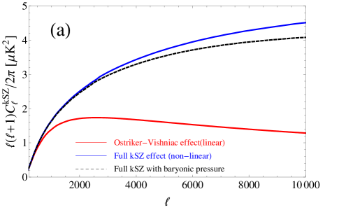
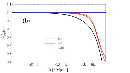
Figure 1: Panel(a): Kinetic SZ effect angular power spectrum $D_{\ell}=\ell(\ell+1)C_{\ell}/2\pi$. Red solid, blue solid and black dashed line corresponds to the Ostriker-Vishniac (OV) effect, full non-linear kSZ effect and the full effect with gas pressure; Panel (b): Window function of gas pressure at different redshifts (Eq. (14)).

In the kSZ power spectrum calculations, it is commonly assumed that the density distribution of the baryonic gas follows exactly that of dark matter, so there is no “bias” in between $\delta_{\rm gas}$ and $\delta_{\rm DM}$ Dodelson & Jubas (1995); Jaffe & Kamionkowski (1998); Ma & Fry (2002); Zhang, Pen, & Trac (2004). However, on small scales, a significant fraction of baryons are in form of gas, thus the thermal pressure of baryons can erase the density fluctuations in the gas distribution on small scales Shaw, Rudd, & Nagai (2012). This “suppression” effect can be modeled as a window function $W(k)$ such that Shaw, Rudd, & Nagai (2012),

$$P^{\rm NL}_{\rm gas}(k,z)=W^{2}(k,z)P^{\rm NL}_{\rm DM}(k,z).$$ (13)

Here we use the fitting formula of $W(k)$ developed by Shaw, Rudd, & Nagai (2012),

$$W^{2}(k,a)=\frac{1}{2}\left\{e^{-k/k_{\rm f}}+\frac{1}{1+[1+g(a)k/k_{\rm f}]^{7/2}}\right\},$$ (14)

where the filter scale $k_{\rm f}=12.6/a+6.3$ and $g(a)=0.84/a$. This fitting formula is proved to provide a better fit to the gas density power spectrum than the analytic formula developed by Gnedin & Hui (1998) through the comparison with “BolshoiNR and L60N” numerical simulations shown in Shaw, Rudd, & Nagai (2012). Thus, by incorporating the gas pressure window function, the power spectrum $\Delta^{2}_{\rm b}(k,z)$ becomes Shaw, Rudd, & Nagai (2012),

$$\Delta^{2}_{\rm b}(k,z) = \frac{k^{3}}{2\pi^{2}}(\dot{a}f)^{2}\int\frac{{\rm d}^{3}\vec{k}^{\prime}}{(2\pi)^{3}}W^{2}(|\vec{k}-\vec{k}^{\prime}|,z)$$ (15)

$$\times P^{\rm NL}_{\delta\delta}(|\vec{k}-\vec{k}^{\prime}|)P_{\delta\delta}(k^{\prime})I(k,k^{\prime}).$$

Note that we assume that the velocity of gas follows exactly the velocity of dark matter, so there is no velocity bias between them.

In Fig. 1, we plot the kSZ angular power spectrum and gas window function in panels (a) and (b) respectively. In Fig. 1 (b), we can see that on the large scales, $W(k)\simeq 1$ while on small scales $W(k)\rightarrow 0$ as $k$ increases due to the gas thermal pressure force. The suppression is not very significant at the onset of the gravitational collapse (high $z$), but as structures gradually collapse, the suppression propagates progressively to larger and larger scales. In Fig. 1 (a), we plot the kSZ angular power spectrum $D_{\ell}\equiv\ell(\ell+1)C_{\ell}/2\pi$ as a function of $\ell$. One can see that the linear OV effect only produces the signal peaking at $\ell\simeq 2000$, and gradually decreases at higher $\ell$. This is because the linear perturbation is sensitive to linear modes which are generically on large scales. One the other hand, using non-linear matter power spectrum instead (Eq. (12)) to calculate the full kSZ effect, one obtains the blue solid line, whose amplitude is about $3$ times higher than that of the linear one on small scales. The $D_{\ell}$ of the full kSZ power spectrum is about $3.06\mu\textrm{K}^{2}$ on scales of $\ell\sim 3000$. In addition, if we incorporate the window function to account for the fact that a fraction of density fluctuations will be suppressed by the gaseous pressure on small scales, i.e. to use Eq. (15), the total signal drops by a factor of $3\%$–$10\%$ on $\ell\sim 2000$ to $10000$.

In order to see clearly how dark energy affects the kSZ signals, in the following analysis, we will adopt the full non-linear kSZ effect without gas pressure as our default model, and discuss the effect of dark energy on this full-kSZ signal. Of-course, when using this model to compare with observations, one needs to consider the effect of gas pressure, which can only be well understood from numerical simulations.

III Dark energy imprints

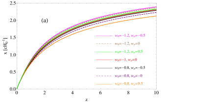
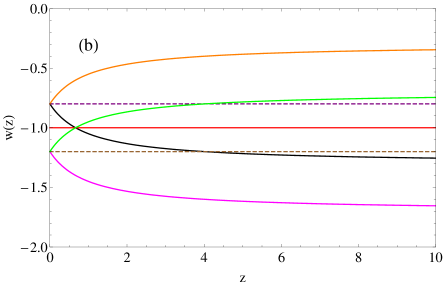
Figure 2: Panel(a): Comoving distance $x=\int^{\infty}_{0}(c/H(z^{\prime})){\rm d}z^{\prime}$ for seven dark energy models with different parameters of EoS. Panel (b): the evolution of EoS for seven dark energy models. The colour scheme of the two panels is shown on panel (a).

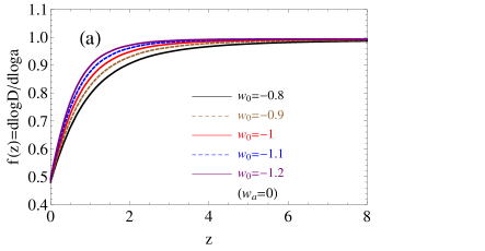
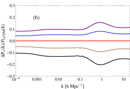
Figure 3: Panel(a): Growth function $f(z)={\rm d}\log(D)/{\rm d}\log(a)$ for the five dark energy models with constant equation of state parameters. Panel (b): the fractional difference of power spectrum $\Delta P_{w}(k)/P_{\rm LCDM}(k)=(P_{w}(k)-P_{\rm LCDM}(k))/P_{\rm LCDM}(k)$ between dark energy models with four different $w$ values and $\Lambda$CDM model. The colour scheme of the two panels is shown on panel (a).

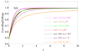
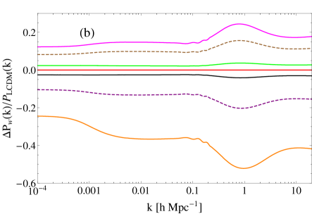
Figure 4: Panel(a): Growth function $f(z)={\rm d}\log(D)/{\rm d}\log(a)$ for the seven dark energy models with time-varying EoS parameters ($w(z)=w_{0}+w_{a}z/(1+z)$). Panel (b): the fractional difference of power spectrum $\Delta P_{w}(k)/P_{\rm LCDM}(k)=(P_{w}(k)-P_{\rm LCDM}(k))/P_{\rm LCDM}(k)$ between dark energy models with six different $w(z)$ evolution and $\Lambda$CDM model. The colour scheme of the two panels is shown on panel (a).

In this section we shall first review how the dark energy EoS changes the comoving distance $x(z)$, and then show how the time-varying dark energy affects the structure growth, and eventually we analyze how the kSZ power spectrum is affected by dark energy.

III.1 EoS $w(z)$ and comoving distance $x(z)$

We adopt the Chevallier-Polarski-Linder (CPL) parametrization Chevallier & Polarski (2001); Linder (2003) of dark energy, i.e., $w(a)=w_{0}+w_{a}(1-a)$ where $w_{0}$ and $w_{a}$ are the two free parameters Hinshaw et al. (2013). In this parametrization form, the fractional matter density and dark energy density evolve as

$$\Omega_{\rm m}(z) = \Omega_{\rm m}^{0}(1+z)^{3},$$

$$\Omega_{\rm DE}(z) = \Omega_{\rm DE}^{0}(1+z)^{3(1+w_{0}+w_{a})}\exp\left(-\frac{3w_{a}z}{1+z}\right),$$ (16)

where $\Omega_{\rm m}^{0}=\Omega_{\rm c}^{0}+\Omega_{\rm b}^{0}$ and $\Omega_{\rm DE}^{0}$ are the matter and dark energy density at present time and their values are set to be the default values in Sec. I. The we can substitute these two equations into the Friedmann equation $H(z)=H_{0}[\Omega_{\rm m}(z)+\Omega_{\rm DE}(z)]^{1/2}$ to calculate the Hubble expansion and comoving distance $x(z)$.

In the following analyses, we take representative values of $w_{0}$ to be $-0.8$, $-0.9$, $-1$, $-1.1$ and $-1.2$, and $w_{a}$ of $-0.5$, $0$ and $0.5$. All these models are allowed by the joint constraints using WMAP9+SPT+ACT+BAO+$H_{0}$ .

In Fig. 2, we plot the dark energy EoS in panel (b) and the corresponding comoving distance at redshift $z$ in panel (a). One can see that the comoving distance increases as $w_{0}$ or $w_{a}$ drops and vice versa. This is simply because a more negative $w_{0}$ or $w_{a}$ means a smaller Hubble parameter in the past, thus a larger comoving distance. This is apparent in Fig. 2 (a).

This brings up the question of degeneracy. If $w_{0}$ is more negative but $w_{a}$ is positive, this will produce the similar effect with a less negative $w_{0}$ but more negative $w_{a}$. For instance, in Fig. 2a, we can see that the $x(z)$ function for $w_{0}=-0.8,w_{a}=-0.5$ is very close to the model $w_{0}=-1.2,w_{a}=0.5$, and also close to the $\Lambda$CDM model ($w_{0}=-1$, $w_{a}=0$). This is because the comoving distance is an integrated effect, although the evolution of $w(z)$ are different for these models, their integrated effects are close to each other. This degenerates between the time-evolving EoS parameters is what we should be aware of when analyzing the kSZ effect signals.

III.2 Growth function $f(z)$

In the 3D power spectrum of kSZ effect (Eq. (15)), $\Delta_{\rm b}(k,z)$ function depends on the evolution of structure growth function $f(z)$, and also the (non)linear matter power spectrum. The growth function $f(z)$ is the logarithmic derivative of the growth rate $D(z)$ ($\delta(t)=D(t)\delta_{0}$), i.e. $f(z)={\rm d}\log(D)/{\rm d}\log(a)$.

We use the numerical code camb CAMB (2000) to calculate the growth function $f$ for various dark energy models in question. Since camb does not output growth function directly, we first modify its subroutine and output the density contrast as a function of redshift, and the calculate its logarithmic derivative to obtain the growth function. Note that we included the dark energy perturbation consistently in the calculation and pay particular attention to the quintom scenario quintom in which $w$ crosses $-1$ during evolution using the prescription in Ref. DEP .

In Fig. 3 (a), we vary the $w_{0}$ value from $-0.8$ to $-1.2$ while fixing $w_{a}=0$, while in Fig. 4 (a), we vary $w_{a}$ as well. One can see that the $f(z)$ function for various models converge at both ends, say, at $z=0$ and $z=10$. This is easy to understand since $f(z)\simeq\Omega_{\rm m}(z)^{\gamma}$ where $\gamma$ has a weak dependence on $w(z)$. At low $z$, $\Omega_{\rm m}(z)\simeq\Omega_{\rm m0}$ while at the high $z$ end, $\Omega_{\rm m}(z)\simeq 1$. Therefore different values of $w_{0}$ or $w_{a}$ mainly affect the evolution in the middle. A more negative $w_{0}$ or $w_{a}$ makes dark energy less important in the past, which effectively gives structures more time to grow before diluted, thus a larger growth rate.

III.3 Power spectrum $P(k)$

We now compare the power spectrum $P(k)$ in different dark energy models.

In Fig. 3 (b) and Fig. 4 (b), we plot the fractional difference of $P(k)$ for different dark energy models with respect to the fiducial $\Lambda$CDM model using the same as in panel (a). One can see that a more negative $w_{0}$ or $w_{a}$,results in a higher $P(k)$ due to a higher growth rate as discussed.

One can also see a small bump on scales of $k\sim 1h{\rm Mpc}^{-1}$, which is due to nonlinearity. For both $w$CDM and $\Lambda$CDM models, there is an enhancement on $P(k)$ on quasi-nonlinear scales (e.g., $k\sim 0.1h{\rm Mpc}^{-1}$) due to the transition from the 2-halo to 1-halo terms. Since this transition scale depends on cosmology, a bump structure can appear on the fractional difference of $P(k)$ between different cosmological models. Another example of such bumps on the same scales can be found in fig. 7 of Ref. Zhao, Li & Koyam (2011), in where $\Delta P/P$ is shown for LCDM cosmology with different values of $\sigma_{8}$.

IV kSZ signal for different dark energy models

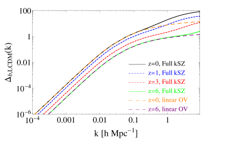
Figure 5: Curl component of momentum power spectrum $\Delta_{\rm b}(k)$ of $\Lambda$CDM model at four different redshifts. The linear OV stands for Ostriker-Vishniac effect (replacing $P^{\rm NL}_{\delta\delta}$ with linear $P_{\delta\delta}$ in Eq. (15)), while the full kSZ corresponds to full non-linear results (using non-linear $P^{\rm NL}_{\delta\delta}$ in Eq. (15)).

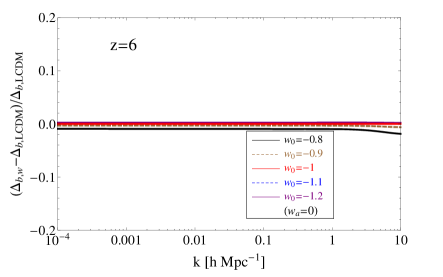
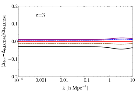
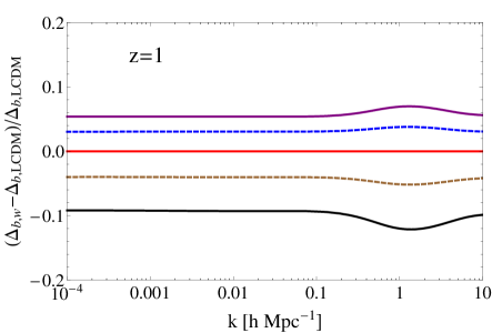
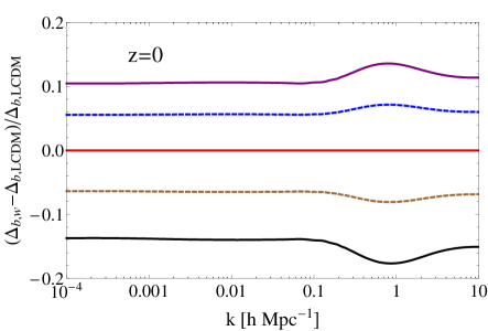
Figure 6: Fractional difference between the power spectrum of curl momentum field $\Delta_{\rm b}(k)$ at four different redshifts. The colour scheme for five different dark energy models with constant EoS is shown on the “$z=6$” panel.

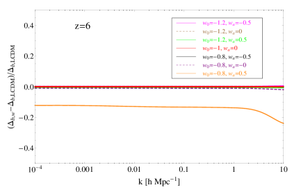
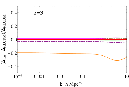
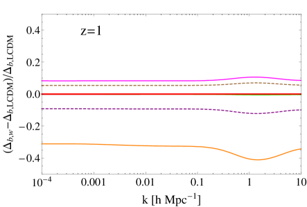
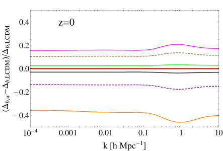
Figure 7: Fractional difference between the power spectrum of momentum field $\Delta_{\rm b}(k)$ at four different redshifts. The colour scheme for seven different dark energy models with time-varying EoS is shown on the “$z=6$” panel.

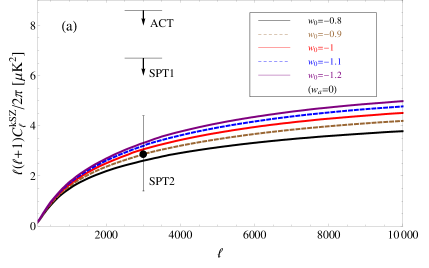
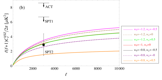
Figure 8: Panel(a): kSZ angular power spectrum ($D_{\ell}\equiv\ell(\ell+1)C^{\rm kSZ}_{\ell}/2\pi$) for five dark energy models with constant EoS. Panel (b): Same as panel (a) but for time-varying dark energy models. The horizontal bars with arrows show $D_{\ell=3000}\leq 8.6\mu\textrm{K}^{2}$ ($95\%$ confidence level) from Atacama Cosmology Telescope (ACT) (2013) and $D_{\ell=3000}\leq 6.7\mu\textrm{K}^{2}$ ($95\%$ CL) from South Pole Telescope (SPT1) Reichardt et al. (2012). The black data point shows $D_{\ell=3000}=2.9\pm 1.5\mu\textrm{K}^{2}$ ($1\sigma$ CL) also from South Pole Telescope (SPT2) while including bispectrum constraints (2013).

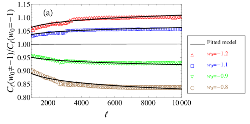
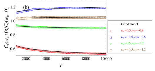
Figure 9: Panel(a): The ratio between $w$CDM and $\Lambda$CDM $C_{\ell}$s (i.e. ratio between model with $w_{0}\neq-1$ and $w_{0}=-1$) with the scaling law (Eqs. (19) and (20)) marked as black lines. Panel (b): the ratio between $C_{\ell}$ with $w_{a}\neq 0$ and with $w_{a}=0$ (note that this is not ratio between dynamical dark energy with $\Lambda$CDM model), the black lines correspond to the scaling law (Eqs. (21) and (22)). The accuracy of the fit is within $1\%$ over $\ell\simeq 3000$–$10000$.

IV.1 3D power spectrum of curl component of momentum field

To calculate the 3D curl momentum power spectrum $\Delta_{\rm b}(k)$ at different redshifts, we rewrite Eq. (12) as,

$$\Delta^{2}_{\rm b}(k,z) = \frac{k^{3}}{2\pi^{2}}(\dot{a}f)^{2}\int\frac{{\rm d}k^{\prime}{\rm d}\mu}{(2\pi)^{2}}P^{\rm NL}_{\delta\delta}(|\vec{k}-\vec{k}^{\prime}|)$$ (17)

$$\times P_{\delta\delta}\tilde{I}(k,k^{\prime}),$$

where

$$\tilde{I}(k,k^{\prime},\mu)=\frac{((k/k^{\prime})^{2}-2\mu(k/k^{\prime}))(1-\mu^{2})}{1+(k/k^{\prime})^{2}-2\mu(k/k^{\prime})},$$ (18)

is the reduced dimensionless kernel function. We plug in the calculation of $f(z)$ and the linear and non-linear matter power spectrum ($P_{\delta\delta}$ and $P^{\rm NL}_{\delta\delta}$) into Eq. (17), and integrate over the cosine angle of separation $\mu=[-1,1]$ and $k^{\prime}$, and then obtain the 3D curl component of momentum power spectrum. We also calculate the OV effect for comparison.

In Fig. 5, we plot the power spectrum of momentum field of the fiducial $\Lambda$CDM model at different redshifts. It is obvious that more and more structures form as the universe evolves, therefore the amplitude of curl momentum power spectrum increases as redshift drops. At high $z$, e.g., $z=6$, the nonlinearity has less effect on the kSZ $\Delta_{\rm b}$ on the concerning scales thus the linear OV approach is a good approximation. However, as the universe evolves, the rms of fluctuation exceeds unity on larger and larger scales, so structures become non-linear on comparatively larger scales. This makes the $z=0$ curl momentum power spectrum significantly different from the OV power spectrum on scales of $k>1\,{h{\rm Mpc}^{-1}}$.

Now we can compare $\Delta_{\rm b}(k)$ of $w$CDM cosmology to that of the $\Lambda$CDM cosmology. In Fig. 6, we plot the fractional difference of $w$CDM momentum power spectrum with the fiducial $\Lambda$CDM model, at four different redshifts, which are chosen as follows: $z=6$ as the onset of structure formation, $z=3$ as the typical epoch of gravitational collapse, $z=1$ as the era when dark energy becomes important, and $z=0$ represents the current epoch. For each panel, we choose $w_{0}$ to be [$-1.2$, $-1.1$, $-1$, $-0.9$, $-0.8$].

One can see that at $z=6$, there is little difference between $w$CDM prediction and the $\Lambda$CDM prediction, since in both scenarios the dark energy component is negligible. The dark energy effect kicks in at $z=1$, making the fractional difference reach $5\%$ at this time. At even later time, this difference become more significant, and at present time this different is $\sim 10\%$.

We show the fractional difference between CPL dark energy model and $\Lambda$CDM model in Fig. 7. One can see that the more negative $w_{0}$ or $w_{a}$ is, the higher the amplitude of curl momentum field is, and vice versa. This is natural since $\Delta_{\rm b}(k)$ increases as the matter power.

IV.2 The total signal

$D_{\ell}(\mu{\rm K}^{2})$	$w_{0}=-0.8$	$w_{0}=-0.9$	$w_{0}=-1$	$w_{0}=-1.1$	$w_{0}=-1.2$
$\ell=1000$	$1.49$	$1.58$	$1.65$	$1.71$	$1.76$
$\ell=2000$	$2.19$	$2.37$	$2.51$	$2.62$	$2.70$
$\ell=3000$	$2.61$	$2.86$	$3.06$	$3.20$	$3.32$
$\ell=4000$	$2.92$	$3.20$	$3.43$	$3.62$	$3.77$
$\ell=5000$	$3.14$	$3.46$	$3.72$	$3.93$	$4.10$
$\ell=6000$	$3.32$	$3.67$	$3.95$	$4.17$	$4.35$
$\ell=7000$	$3.47$	$3.84$	$4.13$	$4.37$	$4.56$
$\ell=8000$	$3.59$	$3.98$	$4.28$	$4.53$	$4.73$
$\ell=9000$	$3.69$	$4.10$	$4.40$	$4.66$	$4.87$
$\ell=10000$	$3.78$	$4.20$	$4.51$	$4.77$	$4.98$

Table 1: The values of kSZ power spectrum $D_{\ell}=\ell(\ell+1)C_{\ell}/2\pi\,[\mu{\rm K}^{2}]$ of $10$ multiples for five constant $w$ models.

$D_{\ell}(\mu{\rm K}^{2})$	$w_{a}=0.5$	$w_{a}=0$	$w_{a}=-0.5$	$w_{a}=0.5$	$w_{a}=0$	$w_{a}=-0.5$
	$w_{0}=-0.8$	$w_{0}=-0.8$	$w_{0}=-0.8$	$w_{0}=-1.2$	$w_{0}=-1.2$	$w_{0}=-1.2$
$\ell=1000$	$0.96$	$1.49$	$1.66$	$1.64$	$1.76$	$1.81$
$\ell=2000$	$1.34$	$2.19$	$2.52$	$2.48$	$2.70$	$2.81$
$\ell=3000$	$1.54$	$2.61$	$3.06$	$3.02$	$3.32$	$3.49$
$\ell=4000$	$1.66$	$2.92$	$3.43$	$3.42$	$3.77$	$3.96$
$\ell=5000$	$1.75$	$3.14$	$3.71$	$3.70$	$4.10$	$4.31$
$\ell=6000$	$1.83$	$3.32$	$3.94$	$3.93$	$4.35$	$4.58$
$\ell=7000$	$1.89$	$3.47$	$4.12$	$4.11$	$4.56$	$4.80$
$\ell=8000$	$1.94$	$3.59$	$4.27$	$4.26$	$4.73$	$4.98$
$\ell=9000$	$1.99$	$3.69$	$4.40$	$4.38$	$4.87$	$5.12$
$\ell=10000$	$2.03$	$3.78$	$4.50$	$4.49$	$4.98$	$5.24$

Table 2: The values of kSZ power spectrum $D_{\ell}=\ell(\ell+1)C_{\ell}/2\pi\,[\mu{\rm K}^{2}]$ of $10$ multiples for varying $w_{a}$ models.

Now we put together the factors of structure growth, comoving distance, and power spectrum of curl momentum field to analyze how dark energy affects the kSZ angular power spectrum.

Note that Eq. (6) is an integral up to $z_{\rm rei}=10$, so it is a projected effect of the velocity field along line of sight. Therefore, we need to count for all the observable modes of fluctuations at different redshifts. By calculating ${\rm d}^{2}C_{\ell}/{\rm d}z{\rm d}\ln k$, Ref. Shaw, Rudd, & Nagai (2012) shows (in their Fig. 1) that, $75\%$ of the full kSZ power comes from redshifts in the range of $[0,7]$ and $k$-mode in the range of $0.2-7.0\,{h{\rm Mpc}^{-1}}$ at $\ell=3000$. This $\{k,z\}$ range is ideal to probe for the amplitude and even the time evolution of the dark energy EoS, thus the kSZ measurement can potentially facilitate a novel test of dark energy. Note that although in the following we plot the $C_{\ell}$s up to $\ell\simeq 10000$, most of the constraining power related to cosmology comes from $\ell\simeq 3000$.

In Fig. 8 (a), we plot the kSZ angular power spectrum $\ell(\ell+1)C_{\ell}/2\pi$ as a function of the multipole $\ell$. We show the result for the various dark energy models with a constant EoS from $-0.8$ to $-1.2$. One can see that, since a more negative $w_{0}$ makes the comoving distance $x(z)$, growth function $f(z)$ and amplitude of curl momentum field $\Delta_{\rm b}$(k) coherently larger, the cumulative integral will eventually enhance the total signal $C_{\ell}$ significantly, and vice versa. On scales of $\ell\sim 3000$, $C_{\ell}(w=-0.8)$ is smaller than the $\Lambda$CDM value by a factor of $14.7\%$, while $C_{\ell}(w=-1.2)$ is larger than the $\Lambda$CDM value by a factor of $8.5\%$. So the total variation of signal given the allowed parameter space by WMAP observations Hinshaw et al. (2013) can reach nearly $23\%$ on scales of $\ell=3000$. On even smaller scales (larger $\ell$’s), the difference can be even more significant. We list the values of $C_{\ell}$’s of $10$ multiples separated by $\Delta\ell=1000$ in Table 1. This is the most prominent effect of dark energy on kSZ power spectrum.

In addition, in Fig. 8 (b), we plot the kSZ power spectrum for dark energy models with a non-zero $w_{a}$, namely, $w_{a}$ from $-0.5$ to $0.5$. Note that this range of $w_{a}$ value is allowed by the joint constrained from WMAP9+SPT+ACT+BAO+$H_{0}$ . We can see that with $w_{0}=-0.8$ or $w_{0}=-1.2$, if $w_{a}>0$ the dark energy kicks in earlier than $w_{a}=0$, so the structure growth will be suppressed and vice versa. Quantitatively, the change in $w_{a}$ by $\pm 0.5$ results in a change in the kSZ signal by a factor of $50$ to $60\%$ on scales of $\ell=3000$, which is a significant effect manifesting the properties of dark energy. We list the $10$ values of $C_{\ell}$’s for CPL dark energy model in Table 2.

To use the kSZ measurements to constrain dark energy EoS, one needs to calculate the kSZ power spectra for a large numbers of cosmological models for the Markov Chain Monte Carlo (MCMC) process. This is computationally expensive so it is useful to develop accurate fitting formula for the practicality.

To understand the feature of kSZ spectrum, we plot the ratio of the spectrum between the constant-$w$ model and the $\Lambda$CDM in Fig. 9 (a) where dots in different colours represent different values of $w$. We can see that the trend of $C_{\ell}(w\neq-1)/C_{\ell}(w=-1)$ close to a power law shape, so we model the function as

$$\frac{C_{\ell}(w\neq-1)}{C_{\ell}(w=-1)}=B\left(\frac{\ell}{1000}\right)^{C},$$ (19)

where the amplitude $B$ and the power index $C$ are to be determined. We first output the left-hand-side of Eq. (19) for each $\ell$, and then by assuming a form of $B$ and $C$ as $a_{1}+a_{2}\exp(w)+a_{3}w$, we fit these parameters with the data $C_{\ell}(w\neq-1)/C_{\ell}(w=-1)$. We find that the following function can very well approximate the function,

$$B = 2.84-3.08\exp(w)+0.70w,$$

$$C = 0.49-0.83\exp(w)+0.19w.$$ (20)

In Fig. 9 (a), we compare the exact numerical results of $C_{\ell}(w)/C_{\ell}(\Lambda{\rm CDM})$ as colour dots with the above fitting formula (Eqs. (19) and (20)) as black solid lines. One can find an excellent agreement between the two.

Furthermore, we investigate the empirical relation between $w_{0}$-$w_{a}$ dark energy kSZ signal with fiducial $\Lambda$CDM model. In Fig. 9 (b), we plot the ratio between the kSZ power spectrum with $w_{a}\neq 0$ and the one with $w_{a}=0$. The colour scheme represents different values of ($w_{0}$, $w_{a}$). One can see that this ratio function is also close to a power law form, we therefore parameterize it as

$$\frac{C_{\ell}(w_{a}\neq 0)}{C_{\ell}(w_{a}=0)}=B^{\prime}\left(\frac{\ell}{1000}\right)^{C^{\prime}}.$$ (21)

Then we find that if allowing $B^{\prime}$ and $C^{\prime}$ related to a parameter $\tilde{x}=w_{a}/w_{0}$, then the ratio function can be well approximated by (by using the same fitting method as described above)

$$B^{\prime}(\tilde{x}) = 22.43+21.35\tilde{x}+10.78\tilde{x}^{2}$$

$$+ 4.84\tilde{x}^{3}-21.43\exp(\tilde{x}),$$

$$C^{\prime}(\tilde{x}) = 5.58(1-\exp(\tilde{x}))+5.55\tilde{x}$$ (22)

$$+ 2.8\tilde{x}^{2}+1.25\tilde{x}^{3}.$$

In Fig. 9 (b), we compare the numerical values of the ratio function by colour dots and its empirical relation (21) and (22) by black solid lines. We again find an excellent agreement between the two. Therefore, our fitting formulae (Eqs. (19)–(22)) can be used for fast calculation of models with $w_{0}\neq-1$ and $w_{a}\neq 0$. Here, we remind the reader that the scaling relation between $C^{\rm kSZ}_{\ell}$ and other cosmological parameters (e.g. $\Omega_{\rm b}$, $\sigma_{8}$, $z_{\rm rei}$, and $\tau$) is investigated in Shaw, Rudd, & Nagai (2012), so can also be used in fast numerical computation.

IV.3 Observational constraints

We now discuss what current and future observational constraints can be obtained on the kSZ power spectrum and its prospective to constrain dark energy. In (2013), by using 148 GHz and 218 GHz Atacama Cosmology Telescope (ACT) data and fitting the template with contribution from thermal and kinetic SZ effects, infrared sources and radio sources, the $95\%$ level upper limit is found to be $8.6\mu\textrm{K}^{2}$. In Reichardt et al. (2012), the constraint on $D_{\ell=3000}$ is obtained by combining $95$, $150$ and $220$ GHz channel data of SPT. By fitting the template of thermal SZ with the kinetic SZ signal, it is found that $D^{\rm kSZ}_{\ell=3000}<2.8\mu{\rm K}^{2}$ at $95\%$ CL. In addition, if considering the the correlation between thermal SZ effect with cosmic infrared background, this upper limit is loosed to $D^{\rm kSZ}_{\ell=3000}<6.7\mu{\rm K}^{2}$ Reichardt et al. (2012) at $95\%$ CL. Furthermore, by incorporating the bispectrum data from the same three channels of SPT, Ref. (2013) finds that the derived constraints on kSZ amplitude at $\ell=3000$ is $D^{\rm kSZ}_{\ell=3000}=2.9\pm 1.5\mu{\rm K}^{2}$ at $1\sigma$ confidence level (CL.), and $<5.5\mu{\rm K}^{2}$ at $95\%$ CL. We place these upper limits and data point in the two panels of Fig. 8.

By comparing the constraints from (2013), Reichardt et al. (2012) and (2013), we can see that although the constraints are not very strong at current situation, the SPT constraint with bispectrum (black data point on Fig. 8b) already tend to rule out the model with ($w_{0}=-0.8$, $w_{a}=0.5$). In addition, the trend of tightening constraints of kSZ signal is quite obvious given many of the ongoing CMB surveys. In the future, if we can place both upper and lower limit on kSZ power spectrum, it can be used as a powerful tool to constrain EoS of dark energy. In reality, Herschel data can be used to separate the infrared and radio sources in the foreground, and thus improve the constraints on kSZ signal.

IV.4 Relation to patchy reionization

What we modeled above is the homogeneous kSZ signal which comes from the era after reionization $z\lesssim 10$. The total signal of kSZ consists of both homogeneous kSZ signal and the patchy reionization signal with most of its contribution from reionization era. The magnitude of the kSZ power from the second component, i.e. patchy reionization, is strongly related to the process of reionization Zahn et al. (2005); McQuinn et al. (2005), which detail is relatively unknown. For instance, it is unclear whether the reionization is an instantaneous reionization, or two-step reionization, or a double reionization Zahn et al. (2012); (2010). In addition, it is not clear how much contribution of the total kSZ signal from the patchy reionization era. For example, if reionization started at $z=14$ and ended at $z=6$, then it can generate roughly $3\mu{\rm K}^{2}$ of patchy kSZ power (at $\ell\simeq 3000$), while the range $z=[8,12]$ would generate $1.5\mu{\rm K}^{2}$ McQuinn et al. (2005); Shaw, Rudd, & Nagai (2012). Therefore, in order to derive the patchy component of total kSZ signal, it is very important to have a good theoretical modeling of the homogeneous kSZ contribution as was laid out in this paper.

V Conclusion

The nature of dark energy is a mystery in modern cosmology, and its property is characterized by its equation of state (EoS) parameter. Current CMB space-mission such as WMAP and Planck, ground-based CMB experiments such as ACT and SPT, as well as baryon acoustic oscillation experiments from SDSS can set up tight constraints on $w$ parameter if assuming that $w$ is a constant. However, if allowing $w$ to vary, such as $w(a)=w_{0}+w_{a}(1-a)$ (the CPL parametrization), the constraints become weaker while a large region of parameter space is allowed.

In this paper we have calculated the kinetic Sunyaev-Zel’dovich signal for general dark energy models with both the constant-$w$ case, and the CPL parametrization (time-varying $w$) case. We first review the calculation of the kSZ signal for the $\Lambda$CDM model, and extend the analysis for the general dark energy model.

We calculate the curl momentum power spectrum $\Delta_{\rm b}(k)$ at different redshifts, and find that dark energy can affect the amplitude and shape of the gravitational clustering at redshifts $0-3$. Finally, we integrate the curl momentum field from redshift $0$ till the reionization redshift $z_{\rm rei}=10$, and find that if, for example, $w_{0}=-0.8$ the total signal of kSZ can be suppressed by a factor of $\sim 14.7\%$ on scales of $\ell=3000$, while $w_{0}=-1.2$ the total signal of kSZ can be enhanced by a factor of $\sim 8.5\%$ on the same scales. We then vary the parameter $w_{a}$ and find that this parameter is more sensitive to the amplitude and shape of the kSZ signal, and in the range of $w_{a}=\pm 0.5$ ($1\sigma$ constrained parameters space by WMAP9+ACT+SPT+BAO+$H_{0}$), the $w_{a}$ can alter the amplitude of kSZ signal by nearly $60\%$. Therefore, if kSZ signal can be precisely measured, it can be a sensitive test of dark energy.

Finally, in order to fast calculate the kSZ signal in a general dark energy model with a constant $w$ or a time-varying $w$, we model an empirical relation which can precisely recover the values of kSZ power spectrum from numerical calculation. Our fitting formulae (Eqs. (19)-(22)) work very precisely in a large region of parameter space ($w_{0}$, $w_{a}$) and therefore can be useful in the fast computation of $C^{\rm kSZ}_{\ell}$.

VI Acknowledgement

We thank the helpful discussion with Douglas Rudd, Laurie Shaw and Pengjie Zhang. Y.Z.M. is supported by a CITA National Fellowship and the Natural Science and Engineering Research Council of Canada. G.B.Z. is supported by the 1000 Young Talents Fellowship in China, by the 973 Program grant No. 2013CB837900, NSFC grant No. 11261140641, and CAS grant No. KJZD-EW-T01, and by the Strategic Priority Research Program “The Emergence of Cosmological Structures” of the Chinese Academy of Sciences, Grant No. XDB09000000.

Appendix A Derivation of $\chi$ and $\mu_{\rm e}$

In Section II.1, we define $\chi$ as the fraction of the total number of electrons that are ionized. We assume that at $z<z_{\rm rei}$ the hydrogen is completely ionized, and the number of helium electrons ionized is $N_{\rm H_{e}}$, so $N_{\rm H_{e}}$ can take $0$, $1$ and $2$ for neutral, singly and fully ionized helium respectively. In our fiducial model we assume $N_{\rm H_{e}}=0$ at all redshifts. Thus $\chi$ is the ratio between ionized and total number of electrons, i.e.

$$\chi = \frac{\overline{n}_{\rm e,i}}{n_{\rm e}}$$ (23)

$$= \frac{n_{\rm H}+n_{\rm H_{e}}\cdot N_{\rm H_{e}}}{n_{\rm H}+2n_{\rm H_{e}}}.$$

The helium number density is

$$n_{\rm H_{e}}=\frac{Y_{\rm p}}{4X_{\rm p}}n_{\rm H},$$ (24)

where $Y_{\rm p}=0.24$ and $X_{\rm p}=1-Y_{\rm p}$ is the primordial helium and hydrogen abundance. Therefore substituting Eq. (24) into Eq. (23), we obtain

$$\chi=\frac{1-Y_{\rm p}(1-N_{\rm H_{e}}/4)}{1-Y_{\rm p}/2}.$$ (25)

We now calculate the gas density as

$$\rho_{\rm g}=m_{\rm p}n_{\rm H}+m_{\rm H_{e}}n_{\rm H_{e}},$$ (26)

since $m_{\rm H_{e}}\simeq 4m_{\rm p}$, and by using Eq. (24), we obtain

$$n_{\rm H}=\frac{\rho_{\rm g}}{\left(1+\frac{Y_{\rm p}}{X_{\rm p}}\right)m_{\rm H}}.$$ (27)

Since the total electron density is $n_{\rm e}=n_{\rm H}+2n_{\rm H_{e}}$, by using Eq. (24), we obtain

$$n_{\rm e}=\frac{\rho_{\rm g}}{m_{\rm p}\mu_{\rm e}},\text{ }\mu_{\rm e}=\frac{1+Y_{\rm p}/X_{\rm p}}{1+Y_{\rm p}/(2X_{\rm p})}=1.14,$$ (28)

where $\mu_{\rm e}$ is called mean electron weight. Then combining Eqs. (23), (25) and (28), we obtain

$$\overline{n}_{\rm e,i}=\frac{\chi\rho_{g}}{m_{\rm p}\mu_{\rm e}}.$$ (29)

References

- Riess et al. (1998) Riess A. G. et al., 1998, ApJ, 116, 1009.
- Perlmutter et al. (1999) Perlmutter S. et al., 1999, ApJ, 517, 565.
- Hinshaw et al. (2013) Hinshaw G. et al., 2013, ApJS, 208, 19
- Planck results XVI. (2013) Ade P. A. R. et al., 2013, arXiv: 1303.5076 [astro-ph.CO].
- Conley et al. (2011) Conley A. et al., 2011, ApJS, 192, 1.
- Suzuki et al. (2012) Suzuki N. et al., 2012, ApJ, 746, 85.
- Beutler et al. (2011) Beutler F. et al., 2011, MNRAS, 416, 3017
- Padmanabhan et al. (2012) Padmanabhan N. et al., 2012, MNRAS, 427, 2132.
- Anderson et al. (2012) Anderson L. et al., 2012, MNRAS, 427, 3435.
- Blake et al. (2012) Blake C. et al., 2012, MNRAS, 425, 405.
- Keisler et al. (2011) Keisler R. et al., 2011, ApJ, 743, 2
- Das et al. (2011) Das S. et al., 2011, ApJ, 729, 62
- Mak et al. (2012) Mak D. S. Y., Pierpaoli E., Schmidt F. and Macellari N., 2012, Phys. Rev. D., 85, 123513.
- Hajian et al. (2013) Hajian A., Battaglia N., Spergel D. N., Bond J. R., Pfrommer C., Siever J. L., 2013, JCAP, 11, 064.
- Gruzinov & Hu (1998) Gruzinov A., & Hu W. 1998, ApJ, 508, 435
- Fan, Carilli, & Keating (2006) Fan X., Carilli C. L., & Keating B, 2006, ARA&A, 44, 415
- Iliev et al. (2006) Iliev I. T., Mellema G., Pen U.-L., Merz H., Shapiro P. R., & Alvarez M. A. 2006, MNRAS, 369, 1625
- Knox, Scoccimarro & Dodelson (1998) Knox L., Scoccimarro R., & Dodelson S. 1998, Phys. Rev. Lett., 81, 2004
- Cooray (2002) Cooray A., 2002, Phys. Rev. D 65, 083518
- Rubino-Martin, Hernandez-Monteagudo, & Enssli (2004) Rubino-Martin J. A., Hernandez-Monteagudo C., & Enssli T. A., 2004, A&A, 419, 439-447
- McQuinn et al. (2005) McQuinn M., Furlanetto S. R., Hernquist L., Zahn O., & Zaldarriaga M. 2005, ApJ, 630, 643
- Santos et al. (2003) Santos M. G., Cooray A., Haiman Z., Knox L., & Ma C. 2003, ApJ, 598, 756
- Zahn et al. (2005) Zahn O., Zaldarriaga M., Hernquist L., & McQuinn M. 2005, ApJ, 630, 657
- Zahn et al. (2012) Zahn O. et al., 2012, ApJ, 756, 65
- Reichardt et al. (2012) Reichardt C. L. et al., 2012, ApJ, 755, 20.
- Dunkley et al. (2011) Dunkley J. et al., 2011, ApJ, 739, 52.
- Limber (1953) Limber D. N., 1953, ApJ, 117, 134
- Dodelson & Jubas (1995) Dodelson S., & Jubas J. N., 1995, ApJ, 561, 15.
- Jaffe & Kamionkowski (1998) Jaffe A. H., & Kamionkowski M., 1998, Phys. Rev. D., 58, 043001.
- Ma & Fry (2002) Ma C. P., & Fry J. N., 2002, Phys. Rev. Lett., 88, 211301.
- Shaw, Rudd, & Nagai (2012) Shaw L. D., Rudd D. H.; Nagai, D., 2012, ApJ, 756, 15
- Dodelson (2003) Dodelson S., Modern Cosmology (Academic Press, San Diego, 2003).
- Sarkar, Feldman & Watkins (2007) Sarkar D., Feldman H. A., Watkins R., 2007, MNRAS, 375, 691.
- Ostriker & Vishniac (1986) Ostriker J. P.; Vishniac E. T., 1986, Nature, 322, 804.
- Hu (2000) Hu W., 2000, ApJ, 529, 12.
- Zhang, Pen, & Trac (2004) Zhang P., Pen U. L., & Trac H., 2004, MNRAS, 347, 1224.
- CAMB (2000) http://camb.info/
- (38) Feng B., Wang X. L. and Zhang X. M., 2005, Phys. Lett. B 607, 35.
- (39) Zhao G. B., Xia J. Q., Li M., Feng B. and Zhang X., 2005, Phys. Rev. D 72, 123515.
- Zhao, Li & Koyam (2011) Zhao G., Li B., & Koyam K., 2011, Phys. Rev. D, 83, 044007
- Smith et al. (2003) Smith R., 2003, MNRAS, 341, 1311
- Takahashi et al. (2012) Takahashi R., Sato M., Nishimichi T., Taruya A., Oguri M., 2012, ApJ, 761, 152
- Gnedin & Hui (1998) Gnedin N. Y., Hui L., 1998, MNRAS, 296, 44
- Chevallier & Polarski (2001) Chevallier M., & Polarski D., 2011, Int. J. Mod. Phys. D 10, 213.
- Linder (2003) Linder E. V., 2003, Phys. Rev. Lett. 90, 091301.
- (46) http://lambda.gsfc.nasa.gov/
- (47) Sievers J. L. et al., 2013, arXiv: 1301.0824
- (48) Crawford T. M. et al., arXiv: 1303.3535, [astro-ph.CO].
- (49) Pritchard J. R., & Loeb A., 2010, Phys. Rev. D 82, 023006.