A Comparative Study of Giant Molecular Clouds in M51, M33 and the Large Magellanic Cloud

Abstract

We compare the properties of giant molecular clouds (GMCs) in M51 identified by the Plateau de Bure Interferometer Whirlpool Arcsecond Survey (PAWS) with GMCs identified in wide-field, high resolution surveys of CO emission in M33 and the Large Magellanic Cloud (LMC). We find that GMCs in M51 are larger, brighter and have higher velocity dispersions relative to their size than equivalent structures in M33 and the LMC. These differences imply that there are genuine variations in the average mass surface density $\langle\Sigma_{\rm H_{2}}\rangle$ of the different GMC populations. To explain this, we propose that the pressure in the interstellar medium surrounding the GMCs plays a role in regulating their density and velocity dispersion. We find no evidence for a correlation between size and linewidth in any of M51, M33 or the LMC when the CO emission is decomposed into GMCs, although moderately robust correlations are apparent when regions of contiguous CO emission (with no size limitation) are used. Our work demonstrates that observational bias remains an important obstacle to the identification and study of extragalactic GMC populations using CO emission, especially in molecule-rich galactic environments.

1. Introduction

Among the different phases of the interstellar medium (ISM), the dense molecular hydrogen gas is especially deserving of study. It is the primary component by mass of the ISM in the central regions of spiral galaxies, and the principal – perhaps only – site of star formation (e.g. Young & Scoville, 1991). In regions with high pressure and high extinction, the molecular gas may be extensive and diffuse (Elmegreen, 1993), but under more typical interstellar conditions a significant fraction ($\sim 50$%, Sawada et al., 2012) of the molecular gas is organized into discrete cloud complexes with masses of $\sim 10^{4}$ to $10^{6}$ M_⊙ and sizes of $\sim 20$ to 50 pc (Blitz, 1993). The study of these giant molecular clouds (GMCs) is of great importance, since their properties determine whether, where and how stars form.

GMCs in the Milky Way and other nearby galaxies are observed to follow correlations between their size, line width, and CO luminosity. These scaling relations have become a standard metric for comparing molecular cloud populations. As originally formulated by Larson (1981), GMCs exhibit: i) a power-law relationship between their size and velocity dispersion, with a slope of $\sim 0.5$; ii) a nearly linear correlation between their virial mass and mass estimates based on other tracers of H₂ column density, which would seem to imply that the clouds are self-gravitating and in approximate virial balance; and iii) an inverse relationship between their size and volume-averaged density. Solomon et al. (1987, henceforth S87) were subsequently able to measure the coefficients and exponents of these correlations for 273 GMCs in the inner Milky Way, establishing the empirical expressions for “Larson’s Laws” that have become the yardstick for studies of GMCs in other galaxies and in different interstellar environments (e.g. Bolatto et al., 2008, henceforth B08).

While resolved studies of extragalactic GMC populations will become routine with the Atacama Large Millimeter Array (ALMA), the twin requirements of high resolution and high sensitivity mean that obtaining extragalactic datasets comparable to the S87 catalogue has thus far only been feasible for a few nearby galaxies. Using either ${}^{12}{\rm CO}(J=1\to 0)$ or ${}^{12}{\rm CO}(J=2\to 1)$ to trace the molecular gas distribution, wide-field surveys covering a significant fraction of a galactic disk with a linear resolution of $\sim 50$ pc or better have recently been completed for M31, M33, IC10, M64, the Magellanic Clouds, IC342, NGC 6822 and NGC 6946 (Rosolowsky et al., 2007; Engargiola et al., 2003; Gardan et al., 2007; Gratier et al., 2012; Leroy et al., 2006; Rosolowsky & Blitz, 2005; Fukui et al., 2008; Mizuno et al., 2001; Wong et al., 2011; Muller et al., 2010; Gratier et al., 2010; Hirota et al., 2011; Donovan Meyer et al., 2012; Rebolledo et al., 2012). These surveys have found some evidence that the properties of molecular clouds vary with environment and their level of star formation activity. In IC342, the LMC and M33, GMCs with signs of ongoing massive star formation are found to exhibit higher peak CO brightness temperatures than non-star-forming clouds (Hirota et al., 2011; Hughes et al., 2010; Gratier et al., 2012). Other examples include larger linewidths for molecular structures without high-mass star formation (IC342 and M83, Hirota et al., 2011; Muraoka et al., 2009) and in the central regions of galaxies (the Galactic Centre and NGC6946, Oka et al., 2001; Donovan Meyer et al., 2012); a decrease in CO brightness at large galactocentric radii (the Milky Way and M33, Heyer et al., 2001; Gratier et al., 2012); higher mass surface densities in high pressure environments (e.g. M64, Rosolowsky & Blitz, 2005); and a lower CO surface brightness and narrower linewidths for GMCs in dwarf galaxies (e.g. B08, Rubio et al., 1993; Muller et al., 2010; Hughes et al., 2010; Gratier et al., 2010). Yet much of the apparent galaxy-to-galaxy variation in GMC properties could be due to the disparate sensitivity and resolution of the observations and/or methodological differences (as noted by e.g. Sheth et al., 2008). Using a consistent method to identify and measure the properties of $\sim 100$ resolved GMCs in a sample of twelve galaxies, B08 concluded that GMCs in fact demonstrate nearly uniform properties across the Local Group.

In this paper, we compare the properties of GMCs identified using high angular resolution CO surveys of three galaxies: M51, M33 and the LMC. Technically, the main difference between our work and previous comparative studies is that each of our datasets covers a significant fraction of the underlying galactic disk and therefore provides a statistically significant sample of clouds for each galaxy (from $\sim 100$ for M33, to more than $\sim 1500$ for M51, although the precise number depends on the decomposition method). All three datasets have sufficient resolution to resolve individual GMCs, but were obtained either with a combination of single-dish and interferometric observations, or with a single-dish telescope alone. Spatial filtering of large-scale emission should therefore not be of concern. We use a consistent methodology to identify significant emission and decompose it into cloud-like structures, and we explicitly test whether differences in the sensitivity, resolution and gridding scheme of the CO data influence the derived GMC properties. A second important difference is physical: the galaxies targeted by previous GMC studies did not include a massive, grand design spiral galaxy like M51 where the ISM is H₂-dominated over a significant fraction of the galactic disk (e.g. Schuster et al., 2007). Some of the observed uniformity of extragalactic GMC populations may be due to the limited range of interstellar environments where high resolution CO surveys have been conducted to date. In this sense, a comparison between the GMCs in M51, M33 and the LMC is of particular interest, since galactic properties such as the metallicity, strength of the spiral potential and the average interstellar pressure vary significantly between these three galaxies (see also Table 1).

This paper is structured as follows. In Section 2, we briefly describe the origin and characteristics of the CO datasets that we have used. Section 3 describes the approach that we have used to identify GMCs and to determine their physical properties. Our comparative analysis of GMC properties and Larson-type scaling relations is presented in Section 4. Our primary result is that GMCs in the inner disk of M51 have different physical properties to the GMCs in M33 and the LMC. In Section 5, we consider possible physical origins for the differences that we observe, and suggest reasons why our conclusion differs from previous comparative studies of GMC populations (e.g. B08). As part of this discussion, we describe several observational effects that should be considered when intepreting empirical correlations between GMC properties. We summarize the key results of our analysis in Section 6.

2. Molecular Gas Data

2.1. M51

The CO data for M51 were obtained by the Plateau de Bure Arcsecond Whirlpool Survey (PAWS Schinnerer et al., 2013; Pety et al., 2013). PAWS observations mapped a total field-of-view of approximately 270″ $\times$ 170″ in the inner disk of M51 in the ABCD configurations of the Plateau de Bure Interferometers (PdBI) between August 2009 and March 2010. Since an interferometer filters out low spatial frequencies, the PdBI data were combined with observations of CO emission in M51 obtained using the IRAM 30 m single-dish telescope in May 2010. The effective angular resolution of the final combined PAWS data cube is 1$\farcs$16 $\times$ 0$\farcs$97, corresponding to a spatial resolution of $\sim 40$ pc at our assumed distance to M51 (7.6 Mpc, Ciardullo et al., 2002). The data cube covers the LSR velocity range 173 to 769  km s^-1 and the width of each velocity channel is 5  km s^-1. The mean RMS of the noise fluctuations across the survey is $\sim 0.4$ K in a 5.0  km s^-1 channel. The PAWS observing strategy, data reduction and combination procedures, and flux calibration are described by Pety et al. (2013). Here we focus on the properties of M51 clouds relative to the GMC populations of the other low-mass galaxies; for some of our analysis, we also distinguish between GMCs located in the spiral arms and central region of M51, and GMCs in M51’s interarm region. The methods that were used to define these different zones (i.e. arm, interarm and central regions) are described by Colombo et al. (submitted), where we also present the M51 GMC catalogue and conduct a detailed investigation of GMC properties in different environments within M51. A CO integrated intensity image of M51 by PAWS is shown in Figure 1[a]. The total CO luminosity within the PAWS data cube is $9.2\times 10^{8}$  K km s^-1 pc² (Pety et al., 2013). Over the same field-of-view, this agrees with the total CO flux obtained by the BIMA (Helfer et al., 2003) and CARMA (Koda et al., 2011) surveys of M51 to within $10$% (Pety et al., 2013).

2.2. M33

For M33, we use the CO data published by Rosolowsky et al. (2007), which combines observations by the Berkeley-Illinois-Maryland Association (BIMA) array (Engargiola et al., 2003) and the Five College Radio Astronomy Observatory (FCRAO) 14 m single-dish telescope (Heyer et al., 2004). The common field-of-view of the single-dish and interferometer surveys is 0.25 square degrees, covering most of M33’s optical disk. The angular resolution of the combined cube is $13\farcs 2\times 12\farcs 9$, corresponding to a spatial resolution of 53 pc for our assumed distance to M33 of 840 kpc (e.g. Galleti et al., 2004). The data covers the LSR velocity range $[-400,40]$  km s^-1, and the velocity channel width is 2.0  km s^-1. The RMS noise per channel is 0.24 K. A CO integrated intensity image constructed from the M33 data is shown in Figure 1[b]. By summing the emission in the BIMA+FCRAO M33 data cube, we estimate that the total CO luminosity of M33 is $3.2\times 10^{7}$  K km s^-1 pc². This agrees with other recent observational estimates for M33’s total CO luminosity to within $\sim 30$% (see e.g. Gratier et al., 2010; Rosolowsky et al., 2007; Heyer et al., 2004), but is a factor of $\sim 2.5$ higher than the total luminosity obtained by summing the emission within the NRO M33 All-Disk Survey map of CO integrated intensity (Tosaki et al., 2011).

2.3. The Large Magellanic Cloud

The CO data for the LMC were obtained by the Magellanic Mopra Assessement (MAGMA). The MAGMA survey design, data acquisition, reduction procedures and calibration are described in detail by Wong et al. (2011). MAGMA mapped CO cloud complexes that had been identified at lower resolution by NANTEN (Fukui et al., 2008), targeting 114 NANTEN GMCs with CO luminosities greater than $7000$  K km s^-1 pc², and peak integrated intensities greater than $1$  K km s^-1. The combined field-of-view of the MAGMA survey is $\sim 3.6$ square degrees. Although the clouds targeted for mapping represent only $\sim 50$% of the clouds in the NANTEN catalogue, the region surveyed by MAGMA contributes $\sim 80$% of the total CO flux measured by NANTEN. The MAGMA LMC data cube has an effective resolution of 45″, corresponding to a linear resolution of $\sim 11$ pc at the distance of the LMC ($50.1$ kpc, Alves, 2004). The velocity channel width is 0.53  km s^-1, and the total LSR velocity range of the cube is 200 to 305  km s^-1. The average RMS noise per channel across the MAGMA survey is $0.3$ K. A CO integrated intensity image constructed from the MAGMA LMC data is shown in Figure 1[c]. The total CO luminosity within the MAGMA data cube is $5.3\times 10^{6}$  K km s^-1 pc² (Wong et al., 2011). This is $\sim 30$% larger than the total CO flux obtained by the NANTEN survey of the LMC (Fukui et al., 2008) over the same field-of-view. As noted by Wong et al. (2011), some of this discrepany is due to systematic errors in the spectral baselines of the MAGMA cube, which accumulate when summing large numbers of noise channels. Using a smoothed (to 3$\farcm$0) 3$\sigma$ contour mask to identify regions of significant emission in the MAGMA cube yields a total CO flux of $3.2\times 10^{6}$  K km s^-1 pc², which agrees with the NANTEN measurement to within 15%.

Table 1Survey parameters and global properties of M51, M33 and the LMC

Galaxy	Resolution	Vel. Resolution	Distance	Sensitivitya	Inclinationb	Morphologyc	Metallicityd	MBc
	[pc]	[ km s-1]	[Mpc]		[degrees] (Ref)		[12 + log(O/H)] (Ref)	[mag]
LMC	11	0.53	0.05	0.3  K km s-1	35 (1)	SB(s)m	8.26 (1)	-18.0
M33	53	2.0	0.84	3.5  K km s-1	56 (2)	SA(s)cd	8.36 (2)	-18.9
M51	40	5.0	7.6	0.8  K km s-1	22 (3)	SA(s)bc pec	8.55 (3)	-20.6

• RMS integrated intensity, assuming a linewidth corresponding to three spectral channels. For the corresponding mass surface density, these numbers should be multiplied by $4.4$, assuming ${X_{\rm CO}}=2\times 10^{20}$  cm^-2 (K km s^-1)^-1 and a helium contribution of 1.36 by mass.

• References for galaxy inclination: (1) van der Marel & Cioni (2001) (2) Paturel et al. (2003) (HyperLeda) (3) Colombo et al., submitted.

• The reference for galaxy types and magnitudes is de Vaucouleurs et al. (1991).

• References for characteristic metallicity: (1) Marble et al. (2010) (2) Rosolowsky & Simon (2008) (3) Moustakas et al. (2010).

Table 2CO Emission Structures Identified in Data Cubes

Galaxy	Cube	Clouds, $N$ ($L_{\rm CO}[\times 10^{7]}$  K km s-1 pc2)		Islands, $N$ ($L_{\rm CO}[\times 10^{7]}$  K km s-1 pc2)
	($L_{\rm CO}[\times 10^{7]}$  K km s-1 pc2)a	Allb	Resolved	All	Resolved
M51	91.8	1507 (48.65)	971 (43.10)	512 (90.02)	247 (88.05)
M51 arm+centralc	68.0	1100 (40.69)	735 (36.60)	235 (82.10)	122 (81.44)
M51 interarm	21.9	407 (7.96)	236 (6.49)	277 (7.92)	125 (6.60)
M33	3.2	114 (0.86)	75 (0.70)	88 (0.88)	66 (0.78)
LMC	0.53d	481 (0.24)	436 (0.23)	285 (0.31)	267 (0.31)
M51	90.7	879 (52.46)	676 (48.37)	144 (90.23)	98 (89.74)
M51 arm+centralc	66.3	519 (40.01)	417 (37.20)	45 (83.11)	32 (83.00)
M51 interarm	24.4	360 (12.45)	259 (11.16)	99 (7.12)	66 (6.74)
M33	3.3	58 (0.24)	33 (0.20)	38 (0.39)	15 (0.25)
LMC	0.46d	41 (0.38)	16 (0.24)	47 (0.27)	32 (0.24)

• CO flux obtained by summing all the emission within the spectral line cube. Values in the upper half of the table are for the intrinsic resolution cubes; values in the lower half of the table are for the matched resolution cubes.

• The first value in each column is the number of objects (see Section 3); the value in parentheses is the total CO flux that is assigned to the objects. The first column (‘All’) lists all identified objects. The second column (‘Resolved’) lists objects where the size and linewidth measurements can be successfully deconvolved.

• For both the intrinsic and matched resolution cubes, an island decomposition identifies structures that are located across the boundary between the arm and interarm region. We classify all such islands as belonging to the arm+central environment.

• Direct summation may not produce a reliable estimate, see Section 2.3.

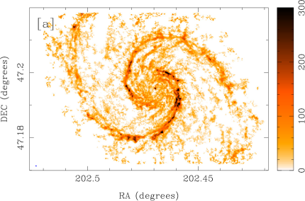
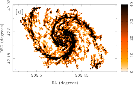
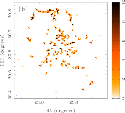
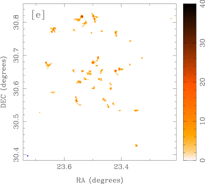
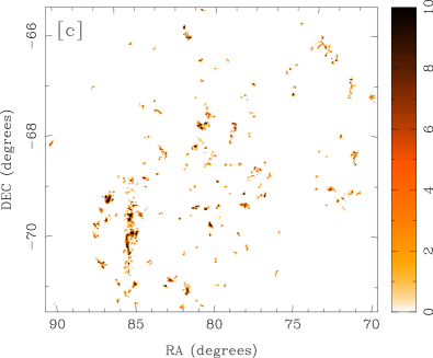
Figure 1.— Maps of CO integrated intensity in [a] M51 (Schinnerer et al., 2013; Pety et al., 2013), [b] M33 (Rosolowsky et al., 2007), and [c] the LMC (Wong et al., 2011). Panels [d] to [f] present the corresponding CO integrated intensity maps after matching the spatial and spectral resolution of the datacubes and interpolating them onto a pixel grid with the same physical dimensions (see text). For all panels, the telescope beam is shown as a blue circle in the bottom left corner. All maps are presented using a square-root intensity scale in  K km s^-1 units. The limits of the colour stretch in panels [a] to [c] are chosen to provide an optimal overview of the spatial distribution of CO emission within each galaxy. In panels [d] to [f], we use the same limits for the intensity scale for each galaxy to highlight the difference in CO brightness between the three galaxies.

3. Cloud Identification

For the identification of significant emission and decomposition of cloud structures within our CO data cubes, we use the algorithm presented by Rosolowsky & Leroy (2006, henceforth RL06), implemented in IDL as part of the CPROPS package. CPROPS uses a dilated mask technique to isolate regions of significant emission within spectral line cubes, and a modified watershed algorithm to assign the emission into individual clouds. Moments of the emission along the spatial and spectral axes are used to determine the size, linewidth and flux of the clouds, and corrections for the finite sensitivity and instrumental resolution are applied to the measured cloud properties. Each step of the CPROPS method is described in detail by RL06.

We adopt the default CPROPS definitions of GMC properties. The cloud radius is defined as $R=1.91\sigma_{\rm R}$ pc, where $\sigma_{\rm R}$ is the geometric mean of the second moments of the emission along the cloud’s major and minor axes. The velocity dispersion $\sigma_{\rm v}$ is the second moment of the emission distribution along the velocity axis, which for a Gaussian line profile is related to the FWHM linewidth, $\Delta v$, by $\Delta v=\sqrt{8\ln 2}\sigma_{\rm v}$. The CO luminosity of the cloud $L_{\rm CO}$ is the emission inside the cloud integrated over position and velocity, i.e.

$$L_{\rm CO}\;[{{\rm\thinspace K\thinspace km\thinspace s}^{-1}\thinspace{\rm pc}^{2}}]=D^{2}\left(\frac{\pi}{180\times 3600}\right)^{2}\Sigma T\delta v\delta x\delta y\;,$$ (1)

where $D$ is the distance to the galaxy in parsecs, $\delta x$ and $\delta y$ are the spatial dimensions of a pixel in arcseconds, and $\delta v$ is the width of one channel in  km s^-1. The mass of molecular gas estimated from the GMC’s CO luminosity $M_{\rm CO}$ is calculated as

$$M_{\rm CO}\;[{{\rm M}_{\odot}}]\equiv 4.4\frac{{X_{\rm CO}}}{2\times 10^{20}[{{\rm\thinspace cm^{-2}\thinspace(K\thinspace km\thinspace s^{-1})}^{-1}}]}L_{\rm CO}\;,$$ (2)

where $X_{\rm CO}$ is the assumed CO-to-H₂ conversion factor, and a factor of 1.36 is applied to account for the mass contribution of helium. The fiducial value of $X_{\rm CO}$ used by CPROPS is ${X_{\rm CO}}=2.0\times 10^{20}$  cm^-2 (K km s^-1)^-1. The virial mass is estimated as

$$M_{\rm vir}\;[{{\rm M}_{\odot}}]=1040\sigma_{\rm v}^{2}R\;,$$ (3)

which assumes that molecular clouds are spherical with truncated $\rho\propto r^{-1}$ density profiles (MacLaren et al., 1988). CPROPS estimates the error associated with a cloud property measurement using a bootstrapping method, which is described in section 2.5 of RL06.

Since molecular clouds exhibit hierarchical structure, it is difficult to identify a scale that uniquely represents their intrinsic physical properties. Recent analyses of extragalactic CO datasets have tended to adopt the recommended CPROPS decomposition parameters for identifying structures with similar properties as Galactic GMCs (i.e. spatial sizes greater than $\sim 10$ pc, linewidths of several  km s^-1, and brightness temperatures less than $\sim 10$ K, e.g. B08, Hughes et al., 2010), but CPROPS offers several tunable parameters that allow the user to modify the kinds of emission structures that are identified by the algorithm. For the comparisons in this paper, we decompose the CO data cubes using two different approaches:

1. Islands: CPROPS identifies all contiguous regions of significant emission within the cube. Significant emission is initially identified by finding pixels with CO brightness $T_{\rm mb}$ above a $4\sigma_{RMS}$ threshold across two adjacent velocity channels, where the RMS noise $\sigma_{RMS}$ is estimated from the median absolute deviation (MAD) of each spectrum. The mask is then expanded to include all connected pixels with $T_{\rm mb}>1.5\sigma_{RMS}$. Islands smaller than a telescope beam are rejected from the catalogue.

2. Clouds: Islands are further decomposed into emission structures that can be uniquely assigned to local maxima that are identified within a moving box with dimensions 150 pc $\times$ 150 pc $\times$ 15  km s^-1. The dimensions of this box are arbitrary: by default, CPROPS uses an $l\times l\times k$ box, where $l$ and $k$ are defined to be three times the beam and channel width respectively. We prefer to adopt a box defined in physical space and apply it uniformly to all three datasets. The emission associated with a local maximum is required to lie at least $2\sigma_{RMS}$ above the merge level with any other maxima, and be larger than the telescope beam. We categorize all such emission regions as distinct clouds. Contrary to the default parameter values, we set the parameter $\textsc{SIGDISCONT}=0$ so that the algorithm makes no attempt to merge the emission associated with pairs of local maxima into a single object.

For both decomposition approaches, the size, linewidth, and flux measurements of each object include extrapolation to a zero-intensity boundary and corrections for the finite spatial and spectral resolution by deconvolving the spatial beam and channel width from the measured cloud size and linewidth respectively. For M51, the cloud decomposition is identical to the method used to construct the PAWS GMC catalogue, which is presented in Colombo et al. (submitted).

4. Results

Figure 2.— A map of CO integrated intensity (black contours) for a subregion of the PAWS field, with the results of the islands (left) and cloud (right) decompositions overlaid. The greyscale image indicates emission that has been assigned to a catalogued structure. The FWHM major and minor axes and the orientation of each structure, as parameterised by CPROPS, are indicated by red and blue ellipses. The black contours represent steps of 50  K km s^-1, with the lowest contour at 20  K km s^-1.

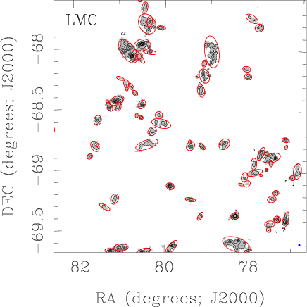
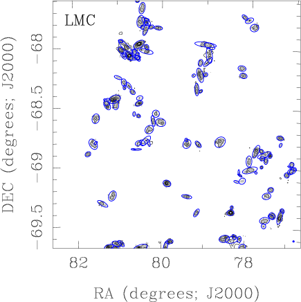
Figure 3.— Same as Figure 2, but for the LMC. The black contours represent CO integrated intensity in steps of 4  K km s^-1, with the lowest contour at 1.5  K km s^-1.

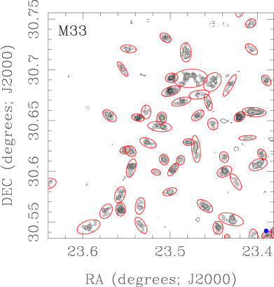
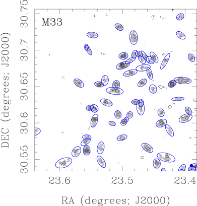
Figure 4.— Same as Figure 2, but for M33. The black contours represent CO integrated intensity in steps of 3  K km s^-1, with the lowest contour at 2  K km s^-1.

4.1. Physical Properties of GMCs

In this section, we compare the basic physical properties (e.g. size, line width, and luminosity) of the cloud structures identified in M51, M33 and the LMC. One advantage of CPROPS over other GMC identification algorithms is that it attempts to correct the cloud property measurements for the finite sensitivity and resolution of the input dataset, and hence reduce some of the observational bias that affects comparisons between heterogeneous datasets. However, resolution and sensitivity should still have considerable impact on whether emission is detected and considered significant, so there may still be some residual bias in the CPROPS results (see RL06 for further discussion). We therefore conduct our analysis on two sets of data cubes, an ‘intrinsic resolution’ set (as described in Section 2) and a ‘matched resolution’ set. In both cases, we work with cloud property measurements that have been extrapolated to the limit of perfect sensitivity, and deconvolved from the instrumental profile (i.e. spatial beam and velocity channel width).

To construct the ‘matched resolution’ dataset, we degraded the M51 and LMC CO data cubes to the same linear resolution as the M33 cube ($\sim 53$ pc), and folded the M33 and LMC datacubes along the velocity axis to the same channel width as the M51 cube ($5\,{{\rm\thinspace km\thinspace s}^{-1}}$). We also interpolated the matched cubes onto an ($x,y$) grid with the same pixel dimensions in physical space ($15\times 15$ pc). The matched M33 and M51 cubes have a similar sensitivity ($0.2$ K per 5  km s^-1 channel), but the LMC cubes are almost an order of magnitude more sensitive. We tried to match the sensitivity of all three matched datasets by adding Gaussian noise at the beam scale to the LMC data, but the emission in the LMC is so faint that CPROPS did not identify any clouds after the noise was increased to this level.

In total, 1507 cloud structures are identified in the intrinsic resolution M51 data cube; 971 clouds have size and linewidth measurements that are deconvolved successfully. These clouds have radii between 5 and 150 pc, velocity dispersions between 0.9 and 31  km s^-1, and peak brightnesses between 1.2 and 16.5 K. For M33 and the LMC, the resolved cloud samples identified in the intrinsic resolution datasets contain 75 and 436 objects respectively. The M33 clouds have radii between 10 and 100 pc, velocity dispersions between 1.2 and 9  km s^-1, and peak brightnesses between 0.7 and 2.8 K, while the LMC clouds have radii between 4 and 40 pc, velocity dispersions between 0.4 and 7  km s^-1, and peak brightnesses between 0.7 and 8.1 K. The median and median absolute deviation (MAD) of the basic physical properties of the clouds identified in the intrinsic resolution datasets for all three galaxies are listed in the upper half of Table 3. We note that the average values of the cloud size and velocity dispersion for each galaxy peak around the spatial and spectral resolution of the data cubes. This is a well-known bias (e.g. Verschuur, 1993) that reflects the hierarchical structure of the ISM from parsec to kiloparsec scales. A peak in the frequency distribution at the resolution limit occurs because structures close to the instrumental resolution are incompletely sampled, whereas larger structures tend to be resolved into smaller objects. As identified in the intrinsic resolution cubes, the trend for clouds in the low mass galaxies to be fainter and have narrower linewidths than clouds in M51 could therefore be mostly due to observational bias. The smaller size and narrower linewidth of the LMC clouds, for example, likely reflects the superior spatial and spectral resolution of the MAGMA survey, while the lower peak brightness of M33 clouds relative to LMC clouds probably arises because the CO emission in M33 suffers more strongly from dilution within the telescope beam (53 pc versus 11 pc, for our adopted distances to M33 and the LMC respectively). Due to resolution bias, it is thus very difficult to determine whether there are significant differences in the cloud populations of the three galaxies using the intrinsic resolution cubes.

The rationale for constructing the matched resolution datacubes is that they allow us to assess whether differences in the M51, M33 and LMC GMC populations exist, even after suppressing resolution bias. It is worth noting, however, that the primary consequence of degrading the M33 and the LMC cubes to a common resolution is to greatly decrease the number of clouds that are identified in the low-mass galaxies. In total, 879, 41 and 58 clouds are identified in the matched resolution cubes for M51, M33 and the LMC, while the corresponding resolved cloud populations (i.e. where the size and linewidth can be successfully deconvolved) contain 676, 16, and 33 objects. The ‘loss’ of resolved clouds from the matched resolution cubes relative to the intrinsic resolution cubes indicates that most of the CO emission in M33 and the LMC exists in structures that are spatially compact and/or have narrow linewidths, and hence diluted in the spatial and/or spectral domain below our detection threshold. Only the largest and brightest CO clouds in M33 and the LMC remain detectable in the matched resolution datasets.

The clouds identified in the M51 matched resolution cube have radii between 9 and 190 pc, velocity dispersions between 0.7 and 28  km s^-1, and peak brightnesses between 0.8 and 13.4 K. In the M33 matched resolution cube, the clouds have radii between 25 and 108 pc, velocity dispersions between 2.5 and 7.6  km s^-1, and peak brightnesses between 0.9 and 2.6 K, while in the LMC matched resolution cube, the clouds have radii between 7 and 116 pc, velocity dispersions between 1.5 and 8.9  km s^-1, and peak brightnesses between 0.3 and 1.6 K. In Figure 5, we plot the distributions of radius, velocity dispersion, peak CO brightness, mass surface density (derived from the CO luminosity assuming a Galactic CO-to-H₂ conversion factor, ${X_{\rm CO}}=2.0\times 10^{20}$  cm^-2 (K km s^-1)^-1), the virial parameter $\alpha\equiv 5\sigma_{\rm v}^{2}R/GM_{\rm CO}$, the scaling coefficient $c\equiv\sigma_{\rm v}/\sqrt{R}$, and the axis ratio for the cloud populations of each galaxy, derived using the matched resolution cubes. The median and MAD of each of the cloud property distributions are listed in the lower half of Table 3.

We test whether the cloud property distributions are similar using a modified version of the two-sided Kolmogorov-Smirnov (KS) test that attempts to account for the uncertainties in the cloud property measurements. In practice, this involves repeating each KS test 500 times, sampling the cloud property measurements within their $3\sigma$ uncertainties using uniform random sampling, rather than only using the measurement reported by CPROPS. The results of these tests are listed in Table 4. We tabulate the median $p$ value, which indicates the probability that measurements in two samples are drawn from the same parent population. We regard median $p$ values of $\langle p\rangle\leq 0.05$ to indicate that there is a statistically significant difference between two distributions.

Table 3Average properties of the resolved GMC populations in M51, M33 and the LMC.

Cloud Propertya	Galaxy/Regionb
	M33	LMC	M51	M51-arm+central	M51-interarm
$R[{\rm pc}]$	$51\pm 13$	$16\pm 5$	$48\pm 14$	$49\pm 14$	$45\pm 14$
$\sigma_{\rm v}[{{\rm\thinspace km\thinspace s}^{-1}}]$	$3.8\pm 0.7$	$1.6\pm 0.4$	$6.4\pm 1.8$	$6.6\pm 1.9$	$5.5\pm 1.5$
$T_{\rm peak}[{\rm K}]$	$1.3\pm 0.2$	$2.0\pm 0.5$	$3.5\pm 1.2$	$3.9\pm 1.4$	$3.0\pm 0.7$
$c\equiv\sigma_{\rm v}/\sqrt{R}[{{\rm\thinspace km\thinspace s}^{-1}}{\rm pc}^{-0.5}]$	$0.5\pm 0.1$	$0.4\pm 0.1$	$0.9\pm 0.3$	$1.0\pm 0.3$	$0.8\pm 0.2$
$\Sigma_{\rm H_{2}}[{{\rm M}_{\odot}\thinspace{\rm pc}^{-2}}]$	$46\pm 20$	$21\pm 9$	$180\pm 82$	$196\pm 90$	$141\pm 53$
$\alpha\equiv\sigma_{\rm v}^{2}R/5GM$	$2.1\pm 0.9$	$2.8\pm 1.2$	$1.6\pm 0.9$	$1.6\pm 0.9$	$1.6\pm 0.9$
Axis Ratio	$1.7\pm 0.3$	$1.6\pm 0.3$	$1.7\pm 0.4$	$1.7\pm 0.4$	$1.6\pm 0.4$
$R[{\rm pc}]$	$46\pm 16$	$57\pm 19$	$67\pm 22$	$71\pm 24$	$60\pm 19$
$\sigma_{\rm v}[{{\rm\thinspace km\thinspace s}^{-1}}]$	$5.4\pm 1.1$	$4.0\pm 0.9$	$6.8\pm 2.0$	$7.4\pm 1.9$	$5.8\pm 1.5$
$T_{\rm peak}[{\rm K}]$	$1.7\pm 0.3$	$0.5\pm 0.2$	$2.8\pm 1.0$	$3.5\pm 1.3$	$2.3\pm 0.6$
$c\equiv\sigma_{\rm v}/\sqrt{R}[{{\rm\thinspace km\thinspace s}^{-1}}{\rm pc}^{-0.5}]$	$0.7\pm 0.2$	$0.5\pm 0.2$	$0.9\pm 0.3$	$0.9\pm 0.3$	$0.8\pm 0.2$
$\Sigma_{\rm H_{2}}[{{\rm M}_{\odot}\thinspace{\rm pc}^{-2}}]$c	$86\pm 44$	$22\pm 7$	$145\pm 66$	$167\pm 77$	$122\pm 49$
$\Sigma_{\rm H_{2}}[{{\rm M}_{\odot}\thinspace{\rm pc}^{-2}}]$d	$124\pm 64$	$34\pm 11$	$116\pm 63$	$134\pm 62$	$98\pm 39$
$\Sigma_{\rm H_{2}}[{{\rm M}_{\odot}\thinspace{\rm pc}^{-2}}]$e	$62\pm 9$	$30\pm 5$	$98\pm 41$	$110\pm 50$	$79\pm 27$
$\alpha\equiv\sigma_{\rm v}^{2}R/5GM$	$2.9\pm 1.3$	$3.1\pm 2.0$	$1.6\pm 0.9$	$1.6\pm 0.9$	$1.6\pm 0.9$
Axis Ratio	$1.6\pm 0.3$	$1.5\pm 0.3$	$1.8\pm 0.4$	$1.8\pm 0.5$	$1.7\pm 0.4$

• Properties were obtained using a cloud-based decomposition (see Section 3). The upper half of the table refers to properties derived from the data cubes at their intrinsic resolution; the results in the lower section refer to the matched cubes.

• We list the median and median absolute deviation (MAD) of the cloud properties for each region. The tabulated values are for resolved clouds.

• Assuming ${X_{\rm CO}}=2\times 10^{20}$  cm^-2 (K km s^-1)^-1 for each population.

• Assuming a galaxy-dependent $X_{\rm CO}$ value, such that the median virial parameter for each galaxy is $\langle\alpha\rangle=2$.

• Assuming a galaxy-dependent $X_{\rm CO}$ value, but for large clouds ($R>50$ pc) only.

Table 4Results for Kolomogorov-Smirnov tests.

Galaxy/Regiona	$R$	$\sigma_{\rm v}$	$T_{\rm peak}$	$c\equiv\sigma_{\rm v}/\sqrt{R}$	$\Sigma_{\rm H_{2}}$b	$\Sigma_{\rm H_{2}}$c	$\Sigma_{\rm H_{2}}$d	$\alpha\equiv\sigma_{\rm v}^{2}R/5GM$	Axis Ratio
LMC - M33	0.73	0.07	$<0.01$	0.10	$<0.01$	$<0.01$	$<0.01$	0.15	0.61
LMC - M51	0.02	$<0.01$	$<0.01$	$<0.01$	$<0.01$	$<0.01$	$<0.01$	$<0.01$	0.07
LMC - M51-arm+central	$<0.01$	$<0.01$	$<0.01$	$<0.01$	$<0.01$	$<0.01$	$<0.01$	$<0.01$	0.04
LMC - M51-interarm	0.14	$<0.01$	$<0.01$	$<0.01$	$<0.01$	$<0.01$	$<0.01$	$<0.01$	0.19
M33 - M51	0.06	0.02	$<0.01$	0.39	0.10	0.48	0.21	0.15	0.25
M33 - M51-arm+central	0.03	$<0.01$	$<0.01$	0.24	0.05	0.42	0.13	0.03	0.16
M33 - M51-interarm	0.16	0.15	$<0.01$	0.53	0.20	0.43	0.44	0.09	0.39
M51-arm+central - M51-interarm	$<0.01$	$<0.01$	$<0.01$	0.03	$<0.01$	$<0.01$	$<0.01$	0.19	0.10

• Properties were obtained using a cloud-based decomposition of the matched resolution cubes (see Section 3). Only resolved clouds (i.e. where the size and linewidth measurements can be successfully deconvolved) are included in the comparison. We tabulate the median $p$-value from 500 repeats of the KS test, where we uniformly sample the cloud property measurements within their $3\sigma$ uncertainties.

• Assuming ${X_{\rm CO}}=2\times 10^{20}$  cm^-2 (K km s^-1)^-1 for each population.

• Assuming a galaxy-dependent $X_{\rm CO}$ value, such that the median virial parameter for each galaxy is $\langle\alpha\rangle=2$.

• Assuming a galaxy-dependent $X_{\rm CO}$ value, but for large $R>50$ pc clouds only.

The KS tests indicate differences in the size and linewidth for clouds in the low-mass galaxies compared to the spiral arm and central regions of M51: on average, clouds in the spiral arms and central region of M51 are larger and have higher velocity dispersions than clouds in M33 and the LMC. This is not just a resolution effect, since these differences are detected in the matched resolution cubes (and, as noted above, the bulk of the cloud population in M33 and the LMC have such small sizes and narrow linewidths that they are not detected in the matched resolution cubes). In the case of the LMC, the tendency for the size and linewidth distributions to extend to low values may be partially due to the MAGMA survey’s higher sensitivity, which allows us to recover a greater proportion of clouds that are small and/or have narrow linewidths. The matched cubes for M33 and M51 have almost identical sensitivity, however, so the differences in the size and linewidth distributions for these galaxies are likely to be physical.

Cloud properties related to CO brightness, such as $T_{\rm peak}$ and $\Sigma_{\rm H_{2}}$, also vary between the three galaxies. The average peak CO brightness of clouds in M51 is significantly higher than in the other galaxies. Assuming that the CO-to-H₂ conversion factor $X_{\rm CO}$ does not vary significantly between the different galaxies, this implies that the mass surface density of a typical cloud in M51 is higher than in M33 and the LMC by a factor of a few. We discuss the assumption of a constant $X_{\rm CO}$ factor in Section 5.1. Once again, the lower average values of $T_{\rm peak}$ and $\Sigma_{\rm H_{2}}$ for the LMC clouds are partly due to the higher sensitivity of the LMC data, which allows us to detect a greater fraction of faint clouds. However, there are no well-resolved ($R>50$ pc) clouds in the matched LMC cubes with $\Sigma_{\rm H_{2}}>50$ M_⊙ pc^-2, even though such clouds would have easily been detected by MAGMA if present. By contrast, 90% of clouds with $R>50$ pc in M51 have $\Sigma_{\rm H_{2}}>50$ M_⊙ pc^-2. This suggests that differences in the $T_{\rm peak}$ and $\Sigma_{\rm H_{2}}$ distributions for the LMC and M51 cloud populations would remain even if we had a more sensitive CO survey of M51. Finally, there appear to be genuine differences between the properties of clouds in different M51 environments: clouds in the interarm region tend to be fainter, and have narrower velocity dispersions than clouds in the spiral arms and central region. A detailed comparison between the properties of clouds within different M51 environments is presented elsewhere (Colombo et al., submitted).

In summary, our analysis suggests that the properties of GMCs are not the same across different galactic environments. More precisely, clouds in the spiral arm and central region of M51 tend to be larger, brighter and have larger velocity dispersions than the clouds in M33 and the LMC. Clouds in the interarm region of M51 tend to be more similar to clouds in the low-mass galaxies. These conclusions hold even after matching the spatial and spectral resolution of the input datacubes and using the same methods to identify and decompose the CO emission into cloud structures.

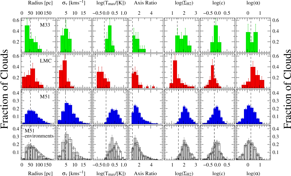
Figure 5.— Histograms of radius, velocity dispersion, peak CO brightness, axis ratio, H₂ mass surface density $\Sigma_{\rm H_{2}}$, the scaling coefficient $c$, and the virial parameter $\alpha$ for clouds in the matched resolution datacubes of LMC, M33 and M51. In the bottom row, we show the distributions for the spiral arm and central regions (black) and interarm region (grey) of M51 separately. The error bars indicate simple counting ($\sqrt{N}$) errors. The dashed vertical lines in the first two columns correspond to resolution limits. For the third and fifth columns, the dashed vertical lines correspond to $4\sigma$ sensitivity limits; for the $\Sigma_{\rm H_{2}}$ sensitivity limit, we further assume that a cloud spans a minimum of three velocity channels and that ${X_{\rm CO}}=2\times 10^{20}$  cm^-2 (K km s^-1)^-1. The dashed vertical lines in the fourth column indicates an axis ratio of 1, i.e. a perfectly round cloud. The dashed vertical lines in the sixth column indicate the value of $c$ that would be expected if clouds have sizes and linewidths corresponding to the spatial and spectral resolution. The dashed lines in the final column indicate $\alpha\equiv 5\sigma_{\rm v}^{2}R/GM_{\rm CO}=2$, which is expected if the kinetic and gravitational energies of the cloud are balanced. For the LMC and M33 distributions, the width of the histogram bins is determined using the Freedman-Diaconis rule, i.e. $h=2{\rm IQR}/n^{1/3}$, where IQR is the interquartile range, $n$ is the number of clouds in the sample, and $h$ is the bin width (Freedman & Diaconis, 1981). We use the same rule to obtain a first estimate of the bin width for the M51 distributions, but we increase the bin width if the increment is finer than our measurement uncertainties would allow us to determine robustly.

4.2. Scaling Relations

Since the very first studies of GMCs in the inner Milky Way (e.g. S87), scaling relations between the physical properties of molecular clouds have become a standard tool for assessing the similarity of GMC populations (e.g. Blitz et al., 2007, B08). We plot the relations between size and linewidth, size and luminosity, and luminosity and virial mass for the objects identified in our M51, M33 and LMC cubes in Figures 6 to 8. In each figure, we also indicate the extragalactic GMCs studied by B08 with small grey crosses; note that we have not re-analysed these data and simply adopt the cloud property measurements published by B08. The relations for clouds identified in the intrinsic and matched resolution data cubes are shown in panels [a] and [b] respectively. Since the GMC identification procedure employed by S87 is most similar to our islands decomposition, we also plot the relations for islands in panels [c] and [d] of each figure.

We assess the strength of scaling relations using the Spearman rank correlation coefficient, $r_{sp}$. We regard $0.3<r_{sp}<0.5$ to indicate a weak correlation, $0.5<r_{sp}<0.75$ to indicate a moderate correlation, and $r_{sp}>0.75$ to indicate a strong correlation. For GMC samples where a correlation between size and linewidth is evident, we estimated the best-fitting power-law $\sigma_{v}=AR^{n}$ using the BCES bisector linear regression method presented by Akritas & Bershady (1996). This method is designed to take measurement errors in both the dependent and independent variable, and the intrinsic scatter of a dataset into account. We use the bisector method because our goal is to estimate the intrinsic relation between the cloud properties (e.g. Babu & Feigelson, 1996). For the measurement errors, we adopt the uncertainties derived by CPROPS. We have assumed that measurement errors in the property measurements are uncorrelated, although some pairs of parameters should have substantial covariance. The resulting fits are tabulated in Table 6. To determine both the correlation strength and the the best-fitting relations, we work with resolved clouds only. We verified that our results are not driven by clouds with poorly determined properties by repeating the calculations using a subsample of resolved clouds where the relative uncertainty in the size and linewidth measurements is less than 50%.

For the cloud decompositions (Figure 6[a] and [b]), there is no compelling evidence for a size-linewidth correlation within any of the galaxies, and the different cloud populations yield $r_{sp}$ between 0.07 and 0.37 (see Table 5). For a composite sample containing all the clouds in M33, M51 and the LMC, $r_{sp}=0.62$ using the $R$ and $\sigma_{\rm v}$ measurements determined from the original data cubes. This good correlation is mostly a consequence of the differences in the spatial and spectral resolutions of the LMC and M51 surveys, however, and disappears once the correlation is determined using a composite cloud sample derived from the matched cubes, for which $r_{sp}=0.18$.

Table 5Spearman rank correlation coefficients for size-linewidth correlations.

Galaxy/Region	$r_{sp}$a	$r_{sp}$b	$r_{sp}$c	$r_{sp}$d	$r_{sp}$e	$r_{sp}$f
Compositeg	0.62	0.18	0.72	0.49	0.69	0.30
M51	0.16	0.16	0.37	0.44	0.26	0.18
M51 arm+central	0.18	0.17	0.41	0.68	0.25	0.46
M51 interarm	0.13	0.07	0.28	0.28	0.21	0.05
LMC	0.37	0.32	0.59	0.45	0.59	0.45
M33	0.33	0.14	0.44	0.05	0.44	0.05

• Cloud decomposition, intrinsic resolution.

• Cloud decomposition, matched resolution.

• Island decomposition, intrinsic resolution, excluding structures with radius greater than 500pc.

• Island decomposition, matched resolution, , excluding structures with radius greater than 500pc.

• Island decomposition, intrinsic resolution, excluding structures with radius greater than 150pc.

• Island decomposition, matched resolution, , excluding structures with radius greater than 150pc.

• Our composite sample consists of all objects in M51, M33 and the LMC.

Table 6Best-fitting parameters for the size-linewidth correlation, $\sigma_{\rm v}=AR^{n}$.

Galaxy/Regiona	Resolution	Decomposition	Coefficient $A$	Index $n$	$\epsilon$b
Composite	Intrinsic	Clouds	$0.06\pm 0.02$	$1.19\pm 0.05$	0.25
Composite	Intrinsic	Islands	$0.11\pm 0.02$	$1.01\pm 0.03$	0.24
M51 arm+centralc	Matched	Islands	$0.46\pm 0.37$	$0.64\pm 0.12$	0.15
M51 arm+centrald	Matched	Islands	$0.34\pm 0.56$	$0.72\pm 0.22$	0.17
LMC	Intrinsic	Islands	$0.16\pm 0.03$	$0.84\pm 0.05$	0.17

• We attempt to fit the size-linewidth relation for cloud samples where the Spearman rank correlation coefficient is greater than 0.5 (see Table 5).

• The final column lists the logarithmic scatter of the residuals about the best-fitting relationship.

• Excludes structures with radius greater than 500pc.

• Excludes structures with radius greater than 150pc.

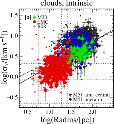
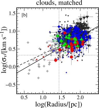
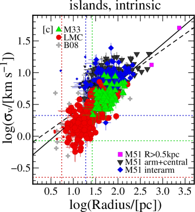
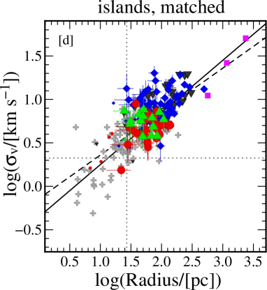
Figure 6.— A plot of radius versus velocity dispersion for objects identified within the CO datacubes for M51, M33, the LMC. Large symbols with error bars indicate resolved clouds where the relative uncertainty in both the size and linewidth measurements is less than 50%; small symbols indicate resolved clouds with larger measurement uncertainties. We omit the error bars on the small symbols for clarity. In panel [a], we plot the relation for clouds identified in the cubes at their intrinsic resolution. The relation for clouds identified in the matched resolution cubes is shown in panel [b]. The relation for island structures are shown in panels [c] and [d] for the decompositions of the original and matched datacubes respectively. Islands with radii greater than $0.5$ kpc (i.e. objects that are much larger than GMCs) are indicated by magenta squares in panels [c] and [d]. In all panels, the black dashed line indicates the relationship derived from the S87 inner Milky Way data, and the black solid line indicates the best-fitting relation for extragalactic GMCs determined by B08. The horizontal and vertical dotted lines indicate the radius and velocity dispersion corresponding to the spatial and spectral resolution of each survey. The sample of extragalactic GMCs analysed by B08 is indicated in each panel by grey crosses.

A stronger relationship between $R$ and $\sigma_{\rm v}$ is apparent for the island decompositions (Figure 6[c] and [d]), with higher $r_{sp}$ values than those obtained using a cloud decomposition for all three galaxies. The size-linewidth relationships for the LMC and the M51 arm+central region yield $r_{sp}$ values greater than 0.5 (see Table 5), indicative of a moderate correlation. We caution, however, that the correlation in the M51 arm+central region may be driven by the largest islands with sizes greater than a few hundred parsecs. Although we have excluded the largest CO-emitting structures in M51 (with $R\gtrsim 0.5$ kpc, represented by magenta squares in Figure 6[c] and [d]) from our correlation and regression analysis, lowering the size threshold to 150 pc tends to make the correlation weaker and to steepen the best-fitting size-linewidth relation (see Table 6). It is remarkable how well the large ($R\gtrsim 200$ pc) island structures in M51 appear to follow the classical S87 size-linewidth relation, since the physical similarity of these structures to Galactic GMCs is remote. We would expect the size-linewidth relationship for GMCs to break down on such large scales, moreover, since existing interpretations for the size-linewidth relation would predict no correlation for non-virialized structures or if an object’s size exceeds the turbulence driving scale. We discuss how the size-linewidth correlation depends on scale and decomposition approach in Section 5.2.2.

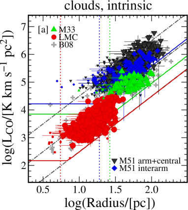
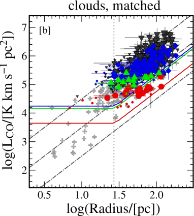
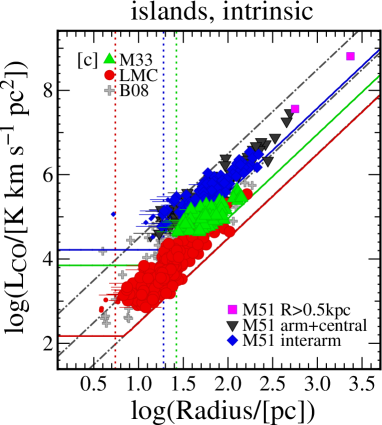
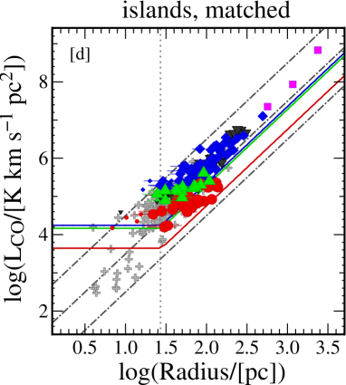
Figure 7.— A plot of radius versus CO luminosity for objects identified within the M51, M33, and LMC data cubes. The panels and plot symbols are the same as in Figure 6. The grey dot-dashed lines indicate constant values of CO surface brightness: ${I(\rm CO)}=1,10,100\,{{\rm\thinspace K\thinspace km\thinspace s}^{-1}}$, which correspond to H₂ mass surface densities of $\Sigma_{\rm H_{2}}=4,44,440$ M_⊙ pc^-2 for ${X_{\rm CO}}=2.0\times 10^{20}$  cm^-2 (K km s^-1)^-1. The solid coloured curves represent an estimate for the $3\sigma$ sensitivity limits of each survey (see also Section 2).

Figure 7 presents the relationship between size and luminosity. Once again, tighter correlations are detected for the island decompositions than for the cloud decompositions. We note that a good correlation between $R$ and $L_{\rm CO}$ is expected since $L_{\rm CO}\approx\sigma_{\rm v}R^{2}\langle T\rangle$ (see Equation 1), and the dynamic range of $R$, $\sigma_{\rm v}$ and $\langle T\rangle$ for each galaxy are limited by the resolution and sensitivity of each survey. The robust-looking correlations in Figure 7 should therefore not be regarded as strong evidence that GMCs have constant mass surface density. In particular, we note that GMCs in each panel typically lie close to the surface brightness sensitivity limits of each survey. It is likely that deeper observations would increase the number of low surface brightness objects detected in each galaxy, and hence increase the scatter in Figure 7.

Despite these biases, Figure 7 indicates genuine variations between the surface brightness of CO-emitting structures in M51 compared to those in the low-mass galaxies. The size and luminosity measurements from the matched cubes of the three galaxies are clearly segregated: GMCs in the low-mass galaxies tend to be smaller and fainter than clouds in M51. For the cloud decomposition of the matched cubes, the median CO surface brightness of well-resolved clouds ($R>50$ pc) in M51 is $28$  K km s^-1. In M51, the variation in surface brightness measurements is also relatively large: the brightest M51 cloud has a CO surface brightness of 347  K km s^-1, more than an order of magnitude above the population’s median value, and 10% of clouds have surface brightness greater than 100  K km s^-1. For well-resolved clouds in M33 and the LMC, by contrast, the median (maximum) CO surface brightness is much lower: 10 (22) and 4 (11)  K km s^-1respectively. While these estimates are biased by the sensitivity of the input datasets, the fact that some M51 clouds achieve CO luminosities more than an order of magnitude higher than clouds of similar size in M33 and the LMC clouds is meaningful. Assuming that the variation in ${X_{\rm CO}}$ between the three galaxies is less than this variation in CO surface brightness, then Figure 7 demonstrates that the molecular structures in M51 reach higher H₂ surface densities than equivalent structures in the low-mass galaxies. We discuss this result – including the effect of ${X_{\rm CO}}$ variations on the derived values of the mass surface density – in Sections 5.1 and 5.2.

The plot of CO luminosity versus virial mass in Figure 8 shows that clouds and islands in all three galaxies are distributed about the line corresponding to ${X_{\rm CO}}=4.0\times 10^{20}$  cm^-2 (K km s^-1)^-1 but with considerable scatter, especially for the cloud decompositions (Figure 8[a] and [b]). A slight vertical offset between the M33, LMC and M51 cloud populations is present in panel [b]: clouds in M33 and the LMC tend to lie above the ${X_{\rm CO}}=4.0\times 10^{20}$  cm^-2 (K km s^-1)^-1 line, while a larger proportion of M51’s cloud population lies on or below it. In previous works, the normalization of the luminosity versus virial mass correlation has been used to estimate the average value of $X_{\rm CO}$ for a GMC population (e.g. Blitz et al., 2007; Fukui et al., 2008). We discuss the results of such a “virial analysis” in Section 5.1, where we investigate possible variations in the $X_{\rm CO}$ factor and their implication for our derived values of the cloud mass surface densities. Strictly, this method requires independent evidence concerning the dynamical state of GMCs, since it assumes that molecular clouds attain virial equilibrium on average (i.e. $\langle\alpha\rangle=1$). In other words, the $X_{\rm CO}$ values corresponding to the diagonal dashed lines in Figure 8 depend on the average value of $\alpha$ that one assumes for the cloud population: if GMCs tend to be globally self-gravitating but not virialised, then $\langle\alpha\rangle\sim 2$ and the mean $X_{\rm CO}$ value that should be inferred from a correlation between luminosity versus virial mass is also smaller by a factor of $\sim 2$. Luminosity ($\sim\sigma_{\rm v}R^{2}\langle T_{\rm CO}\rangle$) and virial mass ($\propto\sigma_{\rm v}^{2}R$) are covariant quantities, so once again the physical significance of the robust-looking correlations in Figure 8 should not be over-interpreted. Nonetheless, the M33, M51 and the LMC data are not located along widely separated tracks in Figure 8, suggesting that the galaxy-wide averages of $X_{\rm CO}$ and $\alpha$ do not deviate from Galactic-like values ($\alpha=1-2$, ${X_{\rm CO}}=2.0-4.0\times 10^{20}$  cm^-2 (K km s^-1)^-1) by more than a factor of a few.

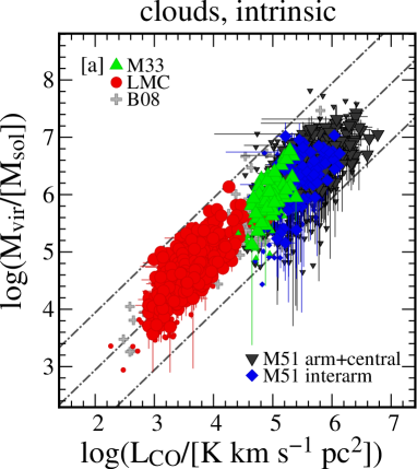
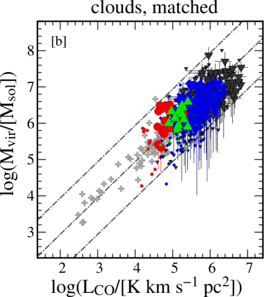
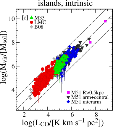
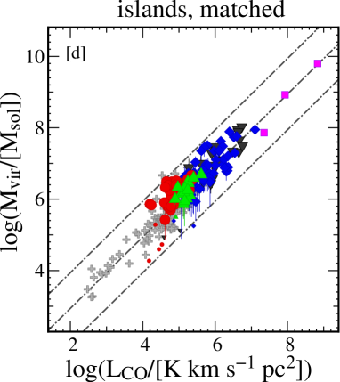
Figure 8.— A plot of virial mass versus CO luminosity for the objects identified in M51, M33, and the LMC. The panels and plot symbols are the same as in Figure 6. The grey dashed lines indicate constant values of the CO-to-H₂ conversion factor, ${X_{\rm CO}}=0.4,4.0,40$  cm^-2 (K km s^-1)^-1.

5. Discussion

5.1. Comparison with Previous Results

Variations between the properties of GMCs in different galaxies are difficult to establish conclusively, and our analysis in Section 4 highlights the risk of conducting comparisons on heterogeneous CO datasets. Nevertheless, we find statistically significant differences between the GMC populations of M51, M33 and the LMC after we account for observational effects (i.e. by using the matched resolution cubes). Namely, GMCs in M51 are intrinsically brighter, and they have larger velocity dispersions and higher mass surface densities than GMCs with comparable size in the two low-mass galaxies. In contrast to many previous studies, our two main conclusions are therefore i) that Larson’s scaling relations are not an especially sensitive tool for comparing the physical properties of GMC populations unless observational and methodological effects are explicitly taken into account, and ii) that the physical properties of GMCs are sensitive to their galactic environment. We discuss the potential nature of this environmental dependence in the remainder of this section, focussing on whether the trends that we observe are better explained by blending (i.e. emission from clouds along the same line-of-sight that overlap in velocity space), galaxy-to-galaxy variations in the CO-to-H₂ conversion factor, or whether they indicate that external pressure plays a role in regulating the physical properties of GMCs. We revisit the interpretation of Larson’s Laws in Section 5.2.

5.1.1 Emission from Overlapping Clouds

In Section 4.1, we found that clouds in the arm+central region of M51 tend to have higher CO peak brightness and larger velocity dispersions than clouds in the two low-mass galaxies and M51’s interarm region. One observational effect that could contribute to this difference is blending of the CO emission from discrete physical entities that overlap in $(x,y,v)$ space, and which cannot be decomposed at our resolution. This effect is unlikely to be dominant in regions where the CO emission is sparsely distributed, and for this reason, blending would seem an improbable explanation for the observed differences between the properties of clouds in M33, the LMC and M51’s interarm environment. On the other hand, clouds may become crowded in M51’s spiral arms. This would tend to increase the size, brightness and velocity dispersion of the structures that our decomposition algorithm identifies in the M51 spiral arm region.

While higher resolution observations – especially in the spectral domain – are required to unambiguously assess the prevalence of blending in M51’s spiral arms, we suggest that blending is unable to fully explain the trends that we observe for several reasons. First, the scale height of the thin molecular disk in M51 is only $\sim 40$ pc (Pety et al., 2013), which makes it unlikely that several $\sim 50$ pc scale structures occuring along a single line-of-sight through the galaxy would be a common phenomenon. Furthermore, even though the typical linewidth of the matched resolution clouds in the arm+central region of M51 is larger than the typical linewidth of clouds in M33, the LMC and in M51’s interarm region, it is still a factor of $\sim 3$ smaller than the cloud-to-cloud velocity dispersion in M51 after we subtract a model of galactic rotation from the cloud radial velocities ($\sim 16$  km s^-1, see Section 5.2.2 for a description of how we subtract a galactic rotation model). This is consistent with the appearance of the CO line profiles in the M51 arm region, which typically exhibit a single peak or, more rarely, two peaks that are well-separated along the velocity axis (which are then identified as discrete clouds by our decomposition algorithm). At our resolution, line profiles with multi-peaked velocity components are rare, even though we might expect a significant number of such profiles if emission in the spiral arms arose from distinct clouds with similar radial velocities that overlapped along the line-of-sight.

A further piece of evidence that the clouds identified in M51’s spiral arms are discrete objects, as opposed to blended emission from multiple overlapping clouds, is that we do not detect any variation in the scaling between the virial mass estimate and CO luminosity for clouds of similar size in the M51 arm and interarm regions. Assuming that blending is not a significant problem in the interarm region – which is likely, since the observed interarm clouds are widely separated in $(x,y)$ space – this agreement suggests that we are identifying discrete clouds in both environments, since mass estimates derived from applying the virial theorem to unbound associations of molecular clouds tend to be significantly greater than the mass inferred from the CO luminosity (e.g. Allen & Lequeux, 1993; Rand, 1995).

Finally, we note that if blending were solely responsible for raising the brightness temperature and velocity dispersion in M51’s arm+central region, then we would expect the effect to be more pronounced in the spiral arms than in the central zone, where the CO emission is more sparsely distributed (see Figure 1[a]). Instead, we observe the opposite: the median peak brightness and velocity dispersion of clouds in the central zone is higher than in the arms by 1.1 K and 0.8  km s^-1 respectively. While this does not imply that blended emission from overlapping clouds is absent, it does suggest that there are physical processes besides – or in addition to – blending that determine the CO emission properties in these environments. In conclusion, although we cannot definitively exclude the possibility that blended emission from overlapping clouds contributes to the higher peak brightness and velocity dispersion of the clouds in the M51 arm+central region, it would seem insufficient to explain all the trends that we describe in Section 4.1.

5.1.2 Variations in the CO-to-H₂ factor

A second potential explanation for the differences between the GMC populations of M51, M33 and the LMC is that there is a systematic difference in the way that ${}^{12}{\rm CO}(J=1\to 0)$ emission traces the underlying H₂ distribution. If this were true, then the underlying physical properties of the molecular (i.e. H₂) clouds might be similar in all three galaxies, despite the variations that we infer from our CO observations. B08, for example, argued that the lower velocity dispersions and CO luminosities of molecular clouds in the Small Magellanic Cloud (SMC) were best understood in terms of selective photodissociation of CO molecules. Feldmann et al. (2012), on the other hand, have argued that ${X_{\rm CO}}$ also increases at high H₂ column densities once the CO-emitting clumps within molecular clouds shadow each other (i.e. when the CO filling factor within a velocity range corresponding to the channel width reaches unity) and CO emission from the cloud becomes globally optically thick.

In general, however, we do not expect large variations in the value of $X_{\rm CO}$ between M51, M33 and the LMC. In a companion paper (Hughes et al., 2013), we argue that the absence of a truncation and the width of the probability distribution functions of CO integrated intensity and brightness provide evidence that the velocity dispersion of the CO-emitting gas within the PAWS field is sufficiently high that the saturation effect described by Feldmann et al. (2012) does not yet apply. Selective CO photodissociation should be an important effect at very low metallicities, but it is not expected to cause large variations in $X_{\rm CO}$ for systems with metal abundances greater than $\sim 0.3Z_{\odot}$ (e.g. Bolatto et al., 2013). The metallicity of M51’s inner disk is approximately solar (e.g. Moustakas et al., 2010; Bresolin et al., 2004), and several independent analyses of dust and molecular line emission in M51 indicate that the $X_{\rm CO}$ factor and dust-to-gas ratio are consistent with local Milky Way values (e.g. Schinnerer et al., 2010; Tan et al., 2011; Mentuch Cooper et al., 2012). M33 and the LMC have a lower metallicity than M51 by a factor of $\sim 2$, but an empirical comparison between the H₂ masses inferred from CO and dust continuum emission also concludes that a Galactic value of the $X_{\rm CO}$ factor is applicable for GMCs in these two low-mass galaxies (Leroy et al., 2011). Based on these studies, we would not expect the $X_{\rm CO}$ factor to vary by more than a factor of a few between all three galaxies.

We can assess whether small variations in the CO-to-H₂ factor could nonetheless account for the differences in the mass surface density of GMCs that we infer using a virial analysis. The median values of the virial parameter in Table 3 are 1.6, 3.1 and 2.9 for resolved clouds in M51, the LMC and M33 respectively. These values are obtained under the assumption that ${X_{\rm CO}}=2\times 10^{20}$  cm^-2 (K km s^-1)^-1. Alternatively, we can assume that the average dynamical state of GMCs is the same in all three galaxies, and that the differences in the virial parameter instead reflect variations in the true value of $X_{\rm CO}$. This is equivalent to attributing the small vertical offset between the GMC populations in Figure 8[b] to variations in $X_{\rm CO}$, rather than inferring that the average dynamical state of GMCs varies between the different galaxies. If GMCs are typically just self-gravitating, then the median value of the virial parameter for a cloud population is $\langle\alpha\rangle=2$ (e.g. Blitz et al., 2007; Leroy et al., 2011). Imposing this median value of $\alpha$ on all the cloud samples requires $X_{\rm CO}$ values of 1.6, 3.1 and $2.9\times 10^{20}$  cm^-2 (K km s^-1)^-1 for M51, the LMC and M33 respectively.

For resolved clouds identified in the matched resolution cubes, the median mass surface densities that we infer for the LMC, M33, and for M51’s interarm and arm+central environments (assuming ${X_{\rm CO}}=2.0\times 10^{20}$  cm^-2 (K km s^-1)^-1) are 22, 86, 122 and 167 M_⊙ pc^-2. The values that would be obtained using the galaxy-dependent $X_{\rm CO}$ values (i.e. derived under the assumption that $\langle\alpha\rangle=2$) are 34, 124, 98 and 134 M_⊙ pc^-2. We repeated the KS tests on the $\Sigma_{\rm H_{2}}$ distributions that we derive using the galaxy-dependent ${X_{\rm CO}}$ values and tabulate the results in Table 4. We find that there is still a statistically significant difference $(p\leq 0.05$) between the mass surface densities for the LMC clouds and all the other cloud populations, and between clouds in the arm and interarm regions of M51. On the other hand, there is no statistically significant difference between the mass surface density distributions of clouds in M33 and M51 using the galaxy-dependent $X_{\rm CO}$ values. Figure 7 shows that the clouds with CO surface brightness greater than 10  K km s^-1 in M33 are mostly small ($R<50$ pc). If we restrict our virial analysis to clouds that are larger than this, then the median cloud mass surface density (obtained using the galaxy-dependent $X_{\rm CO}$ factor) for M33 reduces to 62 M_⊙ pc^-2, but the difference between the mass surface densities of clouds with $R\geq 50$ pc in M33 and clouds in M51 remains statistically insignificant.

In summary, it is possible that the $X_{\rm CO}$ variations can account for some of the differences between the CO-derived properties of clouds in M33 and M51. The differences in CO-derived GMC properties that we find for the LMC clouds and between the M51 environments, on the other hand, cannot be fully explained by $X_{\rm CO}$ variations that remain consistent with either a virial analysis or independent analyses of dust emission and CO excitation. For these galactic environments, the differences in the CO-derived properties appear to reflect genuine variations in the physical properties of the molecular (i.e. H₂) clouds, and not just the fidelity with which CO emission traces the underlying H₂ distribution.

5.1.3 Variations in the Interstellar Pressure

A third possible explanation for the observed differences between the properties of GMCs in M33, the LMC and the inner disk of M51 is that the typical density of GMCs is regulated by pressure variations in the ambient ISM. Traditionally, a large discrepancy between the high internal pressures of Milky Way GMCs and the much lower kinetic (thermal plus turbulent) ISM pressure has been thought to imply that GMCs are approximately in simple virial equilibrium (i.e. with internal kinetic energy equal to half their gravitational potential energy) and hence largely decoupled from the diffuse interstellar gas that surrounds them (e.g. Blitz, 1993). This line of argumentation has been problematised, however, by renewed attention to other potential sources of confining pressure for clouds, such as ram pressure from inflowing material (e.g. Heitsch et al., 2009) and the (static) weight of surrounding atomic gas (e.g. Heyer et al., 2001), as well as a long history of observations suggesting that pressure confinement is significant for molecular clouds in certain galactic environments, such as the outer Galaxy (e.g. Heyer et al., 2001) and at high latitude (e.g. Keto & Myers, 1986). At the very least, we would expect the internal pressure of molecular clouds to be comparable to the external pressure, otherwise the clouds would be rapidly compressed and/or destroyed.

The higher mass surface density of M51 clouds suggests that they should also have higher internal pressures than clouds in the low-mass galaxies (Section 4.1). We can estimate the internal pressure $P_{int}$ of a molecular cloud according to:

$$\frac{P_{int}}{k}=\rho_{g}\sigma_{\rm v}^{2}=1176\left(\frac{M}{M_{\odot}}\right)\left(\frac{R}{{\rm pc}}\right)^{-3}\left(\frac{\sigma_{\rm v}}{{{\rm\thinspace km\thinspace s}^{-1}}}\right)^{2}\,{{\rm\thinspace cm}^{-3}{\rm\thinspace K}}\,,$$ (4)

where $\rho_{g}$ is the H₂ volume density. For the resolved cloud populations identified in the matched resolution cubes of M33, the LMC and M51, we find median internal pressures of $\langle P_{int}/{k}\rangle\sim 1.9\times 10^{5}$, and $3.0\times 10^{4}$, and $4.3\times 10^{5}$  cm^-3  K respectively. We note that clouds in the spiral arms and central region of M51 tend to have higher internal pressures ($\langle P_{int}/{k}\rangle\sim 5.3\times 10^{5}$  cm^-3  K) than clouds in the interarm region ($\langle P_{int}/{k}\rangle\sim 2.6\times 10^{5}$  cm^-3  K).

The average kinetic pressure in the interstellar gas depends on the weight of the gas layer in the gravitational potential of the total mass (i.e. including gas, stars and dark matter) that lies within the gas layer. Assuming the contribution from dark matter is negligible, we can approximate the external pressure at the boundary of a molecular cloud using the expression for the hydrostatic pressure at the disk midplane derived by Elmegreen (1989) for a two-component disk of gas and stars:

$$P_{ext}=\frac{\pi G}{2}\Sigma_{g}\left(\Sigma_{g}+\frac{\sigma_{g}}{\sigma_{*}}\Sigma_{*}\right)$$ (5)

In this expression, $\Sigma_{g}$ is the neutral (atomic + molecular) gas surface density, $\Sigma_{*}$ is the stellar surface density, and $\sigma_{g}$ and $\sigma_{*}$ are the velocity dispersions of the gas and stars, respectively. This expression for the interstellar pressure accounts for the gravity forces due to the stars and gas, as well as the turbulent and thermal hydrodynamic pressure. It is obtained from the definition of the midplane pressure $P_{midplane}=\rho_{g}\sigma_{g}^{2}$, after substituting $\rho_{g}=\Sigma_{g}/2h_{g}$ and $h_{g}=\frac{\sigma_{g}^{2}}{\pi G\Sigma_{total}}$, where $\rho_{g}$ is the gas density at the midplane, $h_{g}$ is the scale height of the gas, and $\Sigma_{tot}\approx(\Sigma_{g}+(\sigma_{g}/\sigma_{*})\Sigma_{*})$ is an estimate for the total mass surface density within the gas layer.

Since our estimate for $P_{ext}$ involves a combination of quantities, we plot the internal pressure of the GMCs as a function of $\Sigma_{g}$ and $(\sigma_{g}/\sigma_{*})\Sigma_{*}$, i.e. the gas and stellar components of the gravitational potential, in Figure 9[a] and [b] respectively. The origin and typical uncertainty associated with our observational estimates for $\Sigma_{g}$, $\Sigma_{*}$ and $\sigma_{*}$ are discussed below. We adopt a constant gas velocity dispersion $\sigma_{g}=10$  km s^-1 for all galaxies. The motivation for this choice is that a roughly constant gas velocity dispersion of $7-10$  km s^-1 has been reported across the disks of several nearby galaxies (see van der Kruit & Freeman, 2011, and references therein). By contrast, Tamburro et al. (2009) recently found that $\sigma_{g}$ decreases linearly by $3-5$  km s^-1 per $\Delta R_{25}$ beyond the optical radius for a subsample of THINGS galaxies, as well as typical values of $\sigma_{g}\sim 15-20$  km s^-1 inside the optical radius. Assuming $\sigma_{g}=20$  km s^-1 for all galaxies would shift the points in Figure 9[b] by $\sim 0.3$ dex towards higher values along the x-axis, i.e. increasing the contribution of stars to the gravitational potential acting on the gas layer. In addition to M51, M33, and the LMC, we include the GMC populations studied by B08 and the GMCs in M64 and NGC 6946 identified by Rosolowsky & Blitz (2005) and Donovan Meyer et al. (2012), respectively. For these additional datasets, our estimates for $P_{int}/k$ are calculated using the published measurements of the GMC properties, i.e. we do not re-analyse the CO datacubes. The vertical error bars in each panel of Figure 9 reflect the median absolute dispersion of the $P_{int}/k$ values, while the horizontal bars indicate the range of values that are observed across the field-of-view of each CO survey. For the B08 galaxies, the range on the x-axis applies to $R_{gal}<0.4R_{25}$, where $R_{25}$ is the optical radius of the galaxy. We adopt this region based on the GMC positions published by B08. For M51, M33, the LMC, M64 and NGC 6946, the range refers to the field-of-view of the original CO surveys. We note that our estimates of $\Sigma_{*}$, $\Sigma_{g}$ and $\sigma_{*}$ are calculated using radial profiles of these quantities, rather than on a pixel-by-pixel basis.

Figure 9[a] and [b] show that the median internal pressure of the GMCs increases with both the gas and stellar components of the gravitational potential, and that neither the gas nor the stellar term dominates our estimate for the external pressure. We note that a correlation with both quantities is to be expected if the internal pressure of molecular clouds is responding to the external pressure, since both stars and gas contribute to the total mass that determines gravitational force. By contrast, a good correlation with the stellar term would not be expected if the mass surface density of GMCs depends on a process such as the shielding of H₂ molecules against the interstellar radiation field, which depends on the local gas column density only. The robust correlations in both panels of Figure 9 further suggest that a relationship between our estimates for $P_{ext}$ and $P_{int}$ does not follow trivially from a correlation between $\Sigma_{g}$ and the average mass surface density of the GMCs. Although both quantities are measures of the gas surface density, Leroy et al. (2013) have recently shown that due to the clumpiness of the molecular ISM, the CO surface brightness measured on $\sim 50$ pc scales within galactic disks does not necessarily track measurements of the CO surface brightness on large ($\sim$ kpc) scales or using radial profiles, since the latter is a combination of both the intrinsic CO surface brightness of small-scale structures and the filling factor of such structures within the $\sim$ kpc scale region or annulus.

Our estimates for $\Sigma_{*}$ have several sources. For M51, NGC 6946 and the B08 targets, we use the $\Sigma_{*}$ radial profile published by Leroy et al. (2008), which uses an empirically calibrated conversion from the 3.6 $\mu$m intensity to the K-band flux, and then a K-band mass-to-light ratio of 0.5 to convert from the K-band intensity to stellar surface density (Bell & de Jong, 2001). The final calibration (equation C1 in Leroy et al., 2008) is:

$$\Sigma_{*}=280\,{\rm cos}i\,I_{3.6}$$ (6)

where $I_{3.6}$ is the 3.6 $\mu$m intensity in MJy sr^-1 and $i$ is the galaxy inclination. We apply the same method to the Spitzer Local Volume Legacy Survey 3.6 $\mu$m map of M64 (Dale et al., 2009) to obtain a radial profile of $\Sigma_{*}$ in that galaxy, assuming a central position of $\alpha_{2000}=12:56:43.6$, $\delta_{2000}=21:40:59.3$ and an inclination $i=60{{}^{\circ}}$ (García-Burillo et al., 2003). The largest uncertainty in our estimates for $\Sigma_{*}$ is the mass-to-light ratio, which depends on the metallicity, initial stellar mass function, and star formation history of galaxies. Bell et al. (2003) show that K-band stellar mass-to-light ratios vary by 0.1 dex for redder galaxies and 0.2 dex for bluer galaxies like M51. We note that the stellar surface density profiles of NGC 6946 and M51 rise sharply at small galactocentric radii ($R_{gal}\lesssim 1$ kpc), which may reflect the presence of a nuclear bulge. Since Equation 5 is invalid in such regions, we only include galactocentric radii where the stellar surface density follows a roughly exponential profile. For M33, we use the stellar surface density profile at a lookback time of 0.6 Gyr published by Williams et al. (2009, see their figure 4). This profile, which agrees within $\sim 50$% with the mass model of Corbelli (2003) inside our field-of-view ($R_{gal}<5.5$ kpc), was constructed by modelling the star formation histories that best reproduce the colour-magnitude diagrams (CMDs) obtained for four fields in M33, imaged with the Advanced Camera for Surveys on the Hubble Space Telescope. The uncertainties in $\Sigma_{*}$ quoted by Williams et al. (2009) are $\lesssim 0.2$ dex. To estimate $\Sigma_{*}$ in the LMC, we use the stellar surface density map published by Yang et al. (2007), which was constructed using number counts of red giant branch (RGB) and asymptotic giant branch (AGB) stars in the Two Micron All Sky Survey Point Source Catalogue (Skrutskie et al., 2006), and normalized for a total stellar mass of $2\times 10^{9}$ M_⊙ in the LMC (Kim et al., 1998).

To estimate $\Sigma_{g}$, we use radial profiles of H I and CO integrated intensity, assuming ${X_{\rm CO}}=2.0\times 10^{20}$  cm^-2 (K km s^-1)^-1, optically thin H I emission and a helium contribution of 1.36 by mass to convert between measurements of integrated intensity and gas mass surface density. For M51, NGC 6946 and the B08 galaxies, we use the gas radial profiles published by Leroy et al. (2008). For the LMC, we use the radial profiles published by Wong et al. (2009). For M33, we use the radial profiles published by Gratier et al. (2010), re-calculating the molecular gas surface density using ${X_{\rm CO}}=2.0\times 10^{20}$  cm^-2 (K km s^-1)^-1. For M64, we measured radial profiles of the atomic and molecular gas surface densities using the THINGS and BIMA-SONG integrated intensity maps of H I and CO emission (Walter et al., 2008; Helfer et al., 2003), adopting the same central position and inclination as for $\Sigma_{*}$.

With the exception of the LMC, our estimates for $\sigma_{*}$ are based on measurements of the central stellar velocity dispersion obtained by Ho et al. (2009) using the Palomar spectroscopic survey of nearby galaxies (Ho et al., 1995, 1997). For the LMC, we use the velocity dispersion of carbon stars measured by van der Marel et al. (2002). Many studies have indicated that the exponential scale height of stellar disks is roughly constant with galactocentric radius (e.g. van der Kruit & Searle, 1981; de Grijs & Peletier, 1997; Kregel et al., 2002), while $\sigma_{*}$ declines (van der Kruit & Freeman, 2011, and references therein). To estimate $\sigma_{*}$ across each CO survey’s field-of-view, we assume that $\sigma_{*}$ decreases exponentially according to $\sigma_{*}=\sigma_{*,0}\exp\left(-\frac{R_{gal}}{2R_{*}}\right)$ (e.g. Bottema, 1993; Boissier et al., 2003), where $\sigma_{*,0}$ is the central stellar velocity dispersion and $R_{*}$ is the exponential scale length of the stellar disk $R_{*}$. We rely on literature values for $R_{*}$ (see Table 7 for exact references).

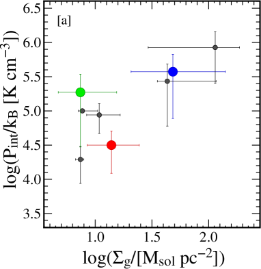
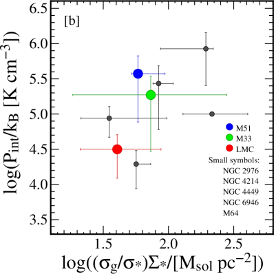
Figure 9.— The median internal pressure of the GMCs in a sample of galaxies where high spatial resolution CO surveys have been conducted versus an estimate of the gas (panel [a]) and stellar (panel [b]) components of the gravitational potential that acts upon the interstellar gas. Large coloured symbols represent M51, M33 and the LMC (this work), while small symbols are for extragalactic GMC populations studied by B08, Rosolowsky & Blitz (2005) and Donovan Meyer et al. (2012). The vertical error bars indicate the median absolute deviation of the internal pressure estimates for each GMC population. The horizontal bars indicate the range of abcissa values that we obtain across the region where GMCs are observed (see text).

Table 7Adopted Parameters to Estimate the External Pressure on GMCs

Galaxy	$\Sigma_{g}$a	$\Sigma_{*}$a	$\sigma_{g}$	$\sigma_{*,0}$	$R_{*}$	$R_{lim}$	Referencesb,c,d,e
	[M⊙ pc-2]	[M⊙ pc-2]	[ km s-1]	[ km s-1]	[kpc]	[kpc]
M51f	[140,40]	[700,225]	10	96.0	2.8	4.2	1,5,7
M33	[15,5]	[590,10]	10	21.0	2.0	5.5	2,3,5,7
LMCg	[8,16]	[175,12]	10	20.0	1.4	3.5	6,7
NGC 2976	[7,7]	[250,90]	10	36.0	0.9	1.5	1,5,8
NGC 4214	[17,8]	[465,50]	10	51.6	0.7	1.2	1,5,8
NGC 4449	[11,8]	[680,125]	10	17.8	0.9	1.1	1,5,8
M64h	[170,5]	[1880,270]	10	96.0	1.1	1.0	4,5,9
NGC 6946f	[115,35]	[500,190]	10	55.8	2.6	4.5	1,5,10

• Values in square brackets indicate the maximum and minimum of the radial profile for galactocentric radii corresponding to the CO survey’s field-of-view.

• References for gas radial profiles: 1. Leroy et al. (2008); 2. Gratier et al. (2010).

• References for stellar radial profiles and stellar disk scale lengths: 1. Leroy et al. (2008); 3. Williams et al. (2009); 4. Regan et al. (2001).

• References for central stellar velocity dispersion: 5. Ho et al. (2009); 6. van der Marel et al. (2002).

• References for GMC properties: 7. this paper; 8. B08; 9. Rosolowsky & Blitz (2005); 10. Donovan Meyer et al. (2012).

• External pressure estimate and radial profiles of gas and stellar surface density exclude the central $\sim 1$ kpc.

• Radial profile of $\Sigma_{*}$ determined by the author using the stellar mass surface density map of Yang et al. (2007).

• Radial profiles of $\Sigma_{g}$ and $\Sigma_{*}$ determined by the author using the THINGS H I survey data (Walter et al., 2008), BIMA-SONG CO survey data (Helfer et al., 2003) and Spitzer Local Volume Legacy Survey 3.6 $\mu$m data for M64 (Dale et al., 2009).

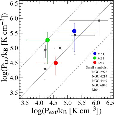
Figure 10.— The median internal pressure of the GMCs in a sample of galaxies where high spatial resolution CO surveys have been conducted versus an estimate of the external pressure within the region surveyed. Plot symbols are the same as in Figure 9. The internal pressures are estimated from GMC properties, the external pressures are estimated from the mass of stars and gas within the disk using an expression derived by Elmegreen (1989) for the total hydrostatic pressure at the disk midplane. The solid diagonal line indicates equality; the dashed diagonal lines indicate where the internal and external pressures differ by an order of magnitude. As in Figure 9, the vertical error bars indicate the median absolute deviation of the internal pressure estimates, while the horizontal bars indicate the range of external pressures in the region where GMCs are observed (see text).

Finally in Figure 10, we plot the median internal pressure of the GMC populations as a function of the external pressure. As in Figure 9, the vertical error bars correspond to the median absolute dispersion of the $P_{int}/k$ measurements of the GMCs in each galaxy, while the horizontal error bars indicate a range of $P_{ext}/{k}$ values that characterise the region of the galactic disk where the GMCs are located. It is clear from Figure 10 that there is a good correlation between the internal and external pressures of GMCs, suggesting that the variation in GMC mass surface densities that we observe between M51, M33 and the LMC may arise because the external ISM pressure plays a role in regulating the internal pressure (and hence velocity dispersion and density) of molecular clouds. Figure 10 further suggests that GMCs are not greatly overpressured with respect to their environment (i.e. $\langle P_{int}/{k}\rangle\sim P_{ext}/{k}$). Rather than simple virial equilibrium between their gravitational and internal kinetic energies, the implication is that GMCs may instead tend towards a pressure-bounded equilibrium configuration. This result is satisfying insofar as it suggests that the traditional dichotomy between strongly gravitationally bound GMCs in the inner disk of the Milky Way and the pressure-confined low-mass clouds in the outer Galaxy and at high galactic latitude may be more apparent than real. If molecular structures are bound by a combination of self-gravity and external pressure, then self-gravity may appear dominant for samples that preferentially include objects with high masses and densities, while pressure confinement should appear more important for samples of low-mass, low density objects. Moreover, the trend in Figure 10 would seem to confirm that the higher GMC mass surface densities and line widths reported by studies of M64 and M82 (Rosolowsky & Blitz, 2005; Keto et al., 2005) – i.e. nearby systems where the disk surface density is intermediate between conditions in Local Group galaxies and true starbursts – arise because GMCs exhibit a continuum of properties (as previously suggested by Rosolowsky, 2007), rather than an intrinsic bi-modality between molecular gas properties in ‘normal’ and ‘starburst’ environments.

An important observable consequence of external pressure regulating the properties of GMCs is that the scaling between a GMC’s size and linewidth – i.e. the coefficient of the size-linewidth relation – should depend on the external pressure. We discuss whether there is evidence for such variations in the GMC populations of M51, M33 and the LMC in Section 5.2.2. Furthermore, if the internal pressure of GMCs is comparable to the interstellar pressure, then this shallow pressure gradient across GMC boundaries means that the clouds’ evolution should be more susceptible to pressure fluctuations in the surrounding ISM than classical GMC models have tended to assume. A detailed investigation of the importance of dynamical pressure for the stability of gas and global patterns of star formation in M51 is the subject of a companion paper (Meidt et al., 2013, see also Jog et al. 2013).

5.2. The Origin of GMC Scaling Relations

Empirical correlations between the size, line width and CO luminosity of Galactic molecular clouds were initially reviewed by Larson (1981). Although their interpretation remains controversial, these scaling relations are regularly used to compare the physical properties of molecular clouds in different galactic environments. A key result of our analysis is that these scaling relations – as obtained from CO surveys of extragalactic GMC populations – are highly dependent on observational effects, such as instrumental resolution and sensitivity, and on the techniques of GMC identification and property measurement that are commonly applied to CO spectral line cubes. In this Section, we discuss some caveats regarding the physical significance of the empirical relations observed for extragalactic GMCs, and whether they are sufficient to demonstrate the universality of GMC properties.

5.2.1 Larson’s Third Law: GMCs have constant H₂ surface densities

Larson’s third “law” describes an inverse relationship between the density of a molecular cloud and its size, implying that molecular clouds have roughly constant molecular gas column density. Several studies of extragalactic GMC populations via their CO emission (e.g. B08) have reported that the average H₂ surface density of extragalactic GMCs is roughly constant within galaxies and, moreover, that it is in good agreement with the value that is observed for GMCs in the inner Milky Way, $\langle\Sigma_{\rm H_{2}}\rangle\sim 100$ M_⊙ pc^-2. Our results in Section 4.2, by contrast, suggest that there are subtle but genuine variations in the characteristic H₂ surface density for the GMC populations of M51, M33 and the LMC.

As noted by several previous authors (e.g. Kegel, 1989; Scalo, 1990; Ballesteros-Paredes & Mac Low, 2002), the limited surface brightness sensitivity of extragalactic CO observations is an evident source of bias for CO-based estimates of GMC mass surface density, since sightlines with low to intermediate H₂ column densities will fall beneath the CO detection limit and hence be excluded from the regions that are identified as molecular. At high brightness, on the other hand, CO observations may underestimate the true H₂ column density if the CO-emitting regions within shadow each other in velocity space (e.g. Feldmann et al., 2012). Coupled with the fact that widefield extragalactic ${}^{12}{\rm CO}(J=1\to 0)$ observations are rarely designed to achieve surface brightness sensitivities much deeper than $5\sigma$ for a typical $\sim 10^{5}$ M_⊙ cloud, these effects suggest that the range of H₂ column densities inferred from CO observations will inevitably be quite restricted. Indeed, even though the minimum CO-derived estimate of $\Sigma_{\rm H_{2}}$ for the PAWS GMCs still likely reflects the survey’s limiting CO surface brightness sensitivity (see Figure 7), the large velocity dispersion of the CO-emitting gas within the PAWS field may explain why the dispersion of the size-CO luminosity relation (and hence the width of the inferred $\Sigma_{\rm H_{2}}$ distribution) is larger for M51 GMCs than for the GMC populations of M33, the LMC and other Local Group systems (cf figure 3 of B08).

Some further insight is provided by comparing the size-luminosity relations obtained using different decompositions of the PAWS data cube in Figure 7. In particular, it is evident that the CO surface brightness values obtained using a method that preferentially identifies structures with a characteristic size scale (i.e. the “cloud-based” decompositions in Figure 7[a] and [b]) cover a wider range than the values obtained when the boundaries of the identified structures are defined using a fixed intensity threshold (i.e. the “island-based” decompositions in Figure 7[c] and [d]). Quantitatively, we find that the scatter in the logarithm of the residuals about the best-fitting size-luminosity relationships increases from $\sim 0.2$ dex for islands in both the intrinsic and matched resolution M51 datacubes to $\sim 0.5$ dex for the cloud structures identified in the same cubes.

These decomposition-dependent results for the scatter in the CO surface brightness (and hence $\Sigma_{H_{2}}$) values derived from the PAWS data are qualitatively similar to the two cases considered by Lombardi et al. (2010) in their analysis of nearby Galactic clouds using dust extinction to trace H₂ column density: the average CO surface brightness of molecular structures above a fixed brightness threshold is approximately constant, while equivalent measurements over a fixed size scale yield much larger variations in $\Sigma_{H_{2}}$, both between and within the GMC populations of the three galaxies that we investigate. Lombardi et al. (2010) argue that the former result arises because molecular clouds have an approximately universal log-normal column density distribution. While this hypothesis can be empirically verified using extinction data for local clouds, the resolution and dynamic range of the extragalactic CO data is insufficient to recover the detailed shape of the $I(\rm CO)$ distribution for individual extragalactic GMCs. In our case, the narrow range of CO surface brightness measurements in Figure 7[c] and [d] arises because a large fraction of the pixels within an island structure sample emission that is close to the observational sensitivity limit. For the intrinsic resolution M51 cube, we find that for over half the islands (51%), pixels with integrated intensity values less than 5$\sigma$ make up more than half the total number of pixels within the structure. This fraction (i.e. where pixels with values $<5\sigma$ consitute the majority of pixels within the structure) is similar in the LMC (46% of islands) and even greater in M33 (78% of islands).

Our conclusion is that the appearance of constant CO surface brightness among extragalactic GMCs is mostly an artifact due to the combination of several conspiring effects: first, the algebraically-imposed covariance of $L_{\rm CO}$ and $R$, which yields a robust yet trivial correlation between these quantities; second, the strategy of designing extragalactic CO surveys to detect a ‘typical’ Milky Way GMC at the $\sim 5\sigma$ level, which limits a survey’s CO surface brightness sensitivity and may only reveal the high-mass, CO-bright GMCs in low-mass galaxies (rather than the bulk of the molecular cloud population); and third, the limited range of environmental conditions that had been probed by extragalactic CO observations with cloud-scale resolution prior to PAWS.

5.2.2 Larson’s First Law: The size-linewith relation

The possibility that the size-linewidth relation is an observational artifact has received less attention in the literature, with most debate focussing on whether it is a sign that GMCs attain approximate virial balance between their gravitational and internal kinetic energies, or a manifestation of interstellar turbulence (see e.g. Ballesteros-Paredes, 2006, and references therein). Nevertheless, our analysis (see Figure 6) suggests that some caution interpreting the extragalactic GMC results is required. In particular, we find little evidence for a correlation between the size and linewidth of cloud structures within M51, M33 or the LMC. A combined sample of GMCs from all three galaxies, on the other hand, yields a size-linewidth relation similar to $\sigma_{\rm v}\propto R^{0.5}$ simply due to the variations in spectral and spatial resolution of the input datasets. For reasons noted in Section 4.1, decomposition algorithms preferentially identify structures in position and velocity space close to the resolution of a data cube. Based on our analysis of the M51, M33 and LMC data, we would therefore recommend that if measurements from high resolution datasets yield the clouds with small radii and narrow linewidths, and low resolution datasets populate the large $R$ and high $\sigma_{\rm v}$ end of a size-linewidth relation, then this bias should be explicitly excluded before a physical explanation for the correlation is invoked.

While cloud structures identified in the matched resolution data cubes of all three galaxies fail to exhibit a strong correlation between their size and linewidth, the vertical offset between the cloud populations in M51 and the low-mass galaxies in Figure 6[b] suggests there may be a genuine difference in the physical state of their cloud populations. More precisely, clouds in M51 – and especially in the spiral arms and central regions – have larger linewidths compared to clouds of an equivalent size in the LMC or M33. Since regions with high velocity dispersion in M51’s inner disk are often associated with low levels of star formation activity (Meidt et al., 2013) and the star formation rates of M33 and the LMC are high relative to their global CO luminosities (assuming a universal molecular gas depletion time of $\sim 2$ Gyr, e.g. Leroy et al., 2008), it seems unlikely that this segregation is due to higher levels of internal turbulence generated by star formation feedback. On the other hand, such an offset would be expected if the dynamical state of the clouds is influenced by the external pressure, as we suggested in Section 5.1. Following Elmegreen (e.g. 1989) (see also Chieze (1987) and Field et al. (2011) for alternative derivations), clouds that achieve equilibrium between self-gravity, the external pressure and their internal kinetic energy should follow:

$$\sigma_{\rm v}\propto\left(\frac{P_{ext}/k_{B}}{10^{4}{{\rm\thinspace cm}^{-3}{\rm\thinspace K}}}\right)^{1/4}\left(\frac{R}{\rm pc}\right)^{1/2}\,.$$ (7)

According to our estimates in Section 5.1, the external pressure experienced by clouds in M51 is approximately an order of magnitude higher than for clouds in M33 and the LMC. From Equation 7, we would then expect M51 clouds to exhibit linewidths $\sim 1.8$ times larger than clouds of similar size in the low-mass galaxies, in good agreement with the vertical offset in the size-linewidth plot that we observe (a factor of $\sim 2$ at a fixed size scale).

A second important result from our analysis in Section 4.2 is that a tighter correlation between the size and linewidth of molecular structures becomes apparent when we identify GMCs as regions of connected CO emission (i.e. islands). Arguably the most convincing example is for islands identified in the LMC data cube with its intrinsic resolution (Figure 6[c]), which follow $\sigma_{\rm v}=(0.16\pm 0.03)R^{0.84\pm 0.05}$ over $\sim 2$ orders of magnitude in size. In the intrinsic resolution cube, island structures in the spiral arms and central region of M51 exhibit a weak correlation that is shallower than for LMC islands: $\sigma_{\rm v}=(1.1\pm 0.4)R^{0.5\pm 0.1}$. On one hand, this could indicate a genuine difference in the density structure of the molecular ISM between the two environments. Numerical simulations by Dobbs & Bonnell (2007) show that if the size-linewidth relation arises due to gas clumps being brought together at the location of a shock (e.g a spiral shock, or the interface of two colliding flows), then a steeper size-linewidth relation is expected if molecular gas is more clumpy. The higher peak brightness of the CO emission in M51 suggests that CO-emitting regions may fill the beam more uniformly in M51 than in the LMC, which is at least qualitatively consistent with the LMC hosting more clumpy molecular material than M51, but higher resolution observations that probe the internal density structure of GMCs in the LMC and M51 would be required to validate this model. On the other hand, we caution that the shallower correlation for islands in M51’s spiral arms may be partly driven by the $\sim 10$ objects with $100<R<500$ pc. Inspection of Figure 6[c] suggests that these objects appear to follow a shallower relationship than the scattered trend exhibited by the smaller islands. Excluding islands with $R>150$ pc from the fit yields $\sigma_{\rm v}=(0.6\pm 0.3)R^{0.6\pm 0.1}$ for the M51 arm+central region, which has a slope that is more similar to the LMC relation.

The possibility that the GMC linewidths that we measure include gas motions unrelated to the cloud’s intrinsic velocity dispersion is underscored by the fact that structures with $R>500$ pc (the magenta squares in Figure 6[c] and [d]) also seem to follow a relation that is roughly consistent with the canonical size-linewidth relationship derived for Galactic GMCs by S87. This is somewhat surprising if the origin of the size-linewidth relation is due to GMCs achieving dynamical equilibrium or turbulence in the molecular ISM, since we would expect the size-linewidth relationship to break down on scales corresponding to the largest virialized structures or the spatial scale on which the turbulence is driven, usually thought to be comparable to the scale height of the gas disk ($\sim 200$ pc in M51). For structures on scales much larger than a typical GMC, the linewidths that we measure are likely to be broadened by systematic motions within the galactic disk, such as galactic rotation or spiral arm streaming motions. To assess the importance of the former effect on the correlations in Figure 6[c] and [d], we subtracted a model of the contribution of galactic rotation to the GMC linewidths from the M51 datacube. In practice, we did this by generating a map of the line-of-sight velocity that would be expected at each spatial position within the PAWS and MAGMA fields from our preferred model of M51’s and LMC’s rotation (Wong et al., 2011; Meidt et al., 2013). After identifying islands of significant emission within the original data cubes, we used the MIRIAD task specshift to offset the individual CO spectra belonging to an island along the spectral axis such that the radial velocity corresponding to the model velocity field at each $(x,y)$ position was shifted to the central channel of a new ‘velocity-shifted’ data cube. This is equivalent to subtracting the modeled rotation component from the observed velocity field map, although we manipulate the data in $(x,y,v)$ space so that the result is a datacube that can be analysed using CPROPS. Next, we estimated the physical properties of each “velocity-shifted” island using the same method that we applied to the original data cubes (see Section 3). The aim of this shifting procedure was to suppress the contribution of galactic rotation to the global velocity dispersion measurement that we obtain for each island.

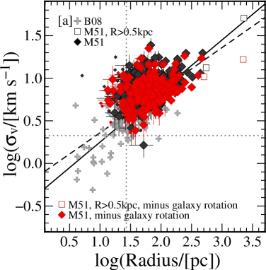
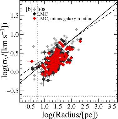
Figure 11.— A plot of radius versus velocity dispersion for islands identified within the [a] M51 and [b] LMC data cubes at their intrinsic resolution. The black points represent measurements obtained directly from the cube and are identical to those shown in Figure 6[c]. The red points represent measurements that were obtained after centring each line profile to the radial velocity expected from a circular rotation model. The black dashed line indicates the relationship derived from the S87 inner Milky Way data, and the black solid line indicates the best-fitting relation for extragalactic GMCs determined by B08. Extragalactic GMCs analysed by B08 are indicated with grey crosses.

In Figure 11, we plot the radius versus the velocity dispersion for the “velocity-shifted” islands (red diamonds) identified in M51 (panel [a]) and the LMC (panel [b]). In both galaxies, there are fewer islands where CPROPS is able to measure the velocity dispersion after the shifting procedure. In M51, many of these objects correspond to islands in the original sample with large velocity dispersions compared to their size, so the outliers and upper envelope of the main distribution of red diamonds in Figure 6 are effectively removed. The result is to bring the bulk of the “velocity-shifted” M51 data points slightly closer to the measurements for the low-mass galaxies, and to the size-linewidth relation for inner Milky Way GMCs (the dashed line in Figure 11). Indeed, a BCES bisector fit to the “velocity-shifted” M51 islands yields $\sigma_{\rm v}=(0.85\pm 0.24)R^{0.51\pm 0.06}$, which is indistinguishable from the canonical S87 result. In the LMC, the data points appear less scattered after the galactic rotation model is subtracted, but the overall distribution is not shifted towards significantly lower velocity dispersions, an effect that is seen for large ($R\gtrsim 300$ pc) islands in M51. The best-fitting size-linewidth relation for the velocity-shifted LMC islands is identical to the relation obtained from islands identified in the original data cube. In summary, we find that contamination of GMC linewidths by systematic motions associated with galactic rotation is significant for the largest CO-emitting structures in M51, but it does not appear to strongly determine the correlation between size and linewidth for structures with spatial scales corresponding to the characteristic size of GMCs (i.e. 10 to 100 pc).

Once again, our conclusion is that further investigation is required to establish whether extragalactic GMC populations follow the same size-linewidth relation as GMCs in the inner Milky Way, and that particular care must be taken to eliminate the effects of resolution, survey design – since the observing configuration of most extragalactic CO surveys is selected to optimise sensitivity to structures with sizes and linewidths similar to Galactic GMCs – and analysis methods. Alternative explanations for the physical origin of the size-linewidth relation – besides simple virial equilibrium and interstellar turbulence – also merit further consideration. Here we have suggested that the larger velocity dispersion of M51 clouds relative to clouds with similar size in the LMC and M33 may be due to the higher pressure at the cloud surface in M51’s inner disk. By contrast, the best explanation for the more robust size-linewidth relations that we recover when we identify GMCs as ‘islands’ of CO emission may be that an islands decomposition yields regions where external processes – such as a converging flow, or a spiral shock – are bringing pre-existing smaller molecular structures into the same spatial location. These ‘cloud associations’ are likely to be globally unbound, with CO linewidths that reflect the macroscopic motions of their constituent gas clumps, rather than interstellar turbulence per se (e.g. Dobbs & Bonnell, 2007). In this case, a scaling between the size and linewidth might simply reflect the inhomogeneous density distribution and velocity fluctuations in the neutral ISM: over small scales, the constituent clumps encounter relatively homogenous material with similar density and local velocity resulting in a low clump-clump velocity dispersion. Over larger scales, however, the clumps interact with material with a larger range of densities and peculiar velocities, and hence experience different decelerations. This produces a higher velocity dispersion between widely-separated clumps. In other words, the tighter correlation between size and linewidth when we identify GMCs as regions of connected CO emission may simply reflect more adequate sampling of the density and velocity structure of the ISM by the dense clumps that constitute the CO islands (e.g. Bonnell et al., 2006).

6. Conclusions

In this paper, we compared the properties of GMCs identified in the PAWS survey of M51’s inner disk to the GMC populations of M33 and the Large Magellanic Cloud (LMC). In contrast to previous comparative studies of extragalactic GMC populations, our datasets contain a statistically significant sample of clouds for each galaxy, have sufficient resolution to resolve individual GMCs and include single-dish measurements to recover total flux information. We explicitly homogenize the resolution, sensitivity and gridding scheme of the CO datasets to suppress these important sources of bias on the derived GMC properties. Our key results are:

1. We find genuine differences in the physical properties of GMCs in M51, M33 and the LMC: on average, GMCs in M51 have higher peak CO brightness, CO surface brightness, and velocity dispersion than GMCs of equivalent size in the low-mass galaxies, consistent with the dynamical state of clouds being influenced by the ambient interstellar pressure. The observed differences are especially pronouced when we restrict our M51 GMC sample to objects in the spiral arm and central region. For this comparison, we took care to homogenize the CO datasets and we note that this procedure was essential to minimize observational bias.

2. The presence of a correlation between size and linewidth depends sensitively on how we define clouds. If we apply an aggressive decomposition algorithm to the CO data cubes, we find no compelling evidence for a correlation between size and line width for the GMC populations of M51, M33 or the LMC. A strong correlation similar to the canonical size-linewidth relationship for GMCs in the inner Milky Way is apparent when we identify GMCs as regions of contiguous CO emission. We propose that these structures are more like cloud associations, i.e. regions where an external process has caused smaller pre-existing molecular gas structures to converge. In addition to simple virial equilibrium or a classical turbulent cascade, the observed size-linewidth relation may also be a reflection of more adequate sampling of the inhomeogeneous density and velocity structure of the interstellar medium by the clouds that belong to these associations. In general, more observational effort to identify the processes that contribute to the global linewidths of molecular clouds in different galactic environments would be highly desirable, and would significantly improve our understanding of the physical origin of the size-linewidth relation.

3. Within M51, M33 and the LMC, CO islands exhibit a relatively narrow range of surface brightness measurements. We argue that the appearance of uniform surface brightness for these structures may be imposed by using a intensity threshold close to the survey’s sensitivity limit to define the island boundary, since for many islands (between 46 and 78% depending on the galaxy), the majority of pixels sample emission that is less than the 5$\sigma$ sensitivity limit.

4. The dynamic range of surface brightness measurements increases for a more aggressive cloud decomposition of the CO datacubes, which tends to retain the high brightness substructure within the islands, and discard the low brightness emission surrounding the high intensity peaks. There appear to be genuine variations in the average surface brightness – and, we infer, average mass surface density – of the GMC populations in M51, M33 and the LMC. Combining our analysis with literature measurements of resolved extragalactic GMC properties suggests that the average GMC mass surface density varies with the characteristic interstellar pressure of the galactic environment where the GMCs are located.

Our results highlight the difficulties and limitations of decomposing molecular gas into clouds. This type of analysis becomes especially problematic for molecule-rich environments – like the inner disk of M51 – where the emission is both bright and extended over spatial scales many times greater than the observational resolution. In light of the sensitive dependence of GMC property measurements and scaling relations on instrumental resolution, observational sensitivity and decomposition approach, methods that can analyse hierarchical structure (e.g. Rosolowsky et al., 2008; Kauffmann et al., 2010; Shetty et al., 2012) would seem to offer a promising approach to studying the physical properties of the molecular ISM, since they can quantify the importance of e.g. self-gravity or external pressure as a function of spatial scale without imposing a cloud-like model for the molecular gas a priori. An analysis of the PAWS data using hierarchical decomposition methods will be presented in a forthcoming paper (Leroy et al., in preparation).

Finally, we note that the tendency for molecular clouds in low-mass galaxies and the outer Milky Way to be smaller and fainter than molecular structures in the inner Milky Way – and, conversely, for GMCs in molecule-rich, high-pressure environments to be denser and more massive than local clouds – was already suggested by several previous observational studies (e.g. Keto & Myers, 1986; Heyer et al., 2001; Oka et al., 2001; Rosolowsky & Blitz, 2005; Gratier et al., 2010; Wong et al., 2011). Firmly establishing a dependence between GMC properties and galactic environment has proven difficult, however, in part because assembling large samples of extragalactic GMCs (especially in CO-faint dwarf galaxies) remains technically challenging with the current generation of millimetre telescopes. Future observations with ALMA that efficiently survey the CO emission across a significant fraction of nearby galactic disks will be invaluable for increasing the number of extragalactic GMC samples and the range of environments where GMC properties can be studied. Such observations will be crucial for establishing the physical mechanisms that are responsible for variations in GMC properties and regulate their ability to form stars.

References

- Akritas & Bershady (1996) Akritas, M. G., & Bershady, M. A. 1996, ApJ, 470, 706
- Allen & Lequeux (1993) Allen, R. J., & Lequeux, J. 1993, ApJ, 410, L15
- Alves (2004) Alves, D. R. 2004, New Astronomy Review, 48, 659
- Babu & Feigelson (1996) Babu, G. J., & Feigelson, E. D. 1996, Astrostatistics, ed. Babu, G. J. & Feigelson, E. D.
- Ballesteros-Paredes (2006) Ballesteros-Paredes, J. 2006, MNRAS, 372, 443
- Ballesteros-Paredes & Mac Low (2002) Ballesteros-Paredes, J., & Mac Low, M.-M. 2002, ApJ, 570, 734
- Bell & de Jong (2001) Bell, E. F., & de Jong, R. S. 2001, ApJ, 550, 212
- Bell et al. (2003) Bell, E. F., McIntosh, D. H., Katz, N., & Weinberg, M. D. 2003, ApJS, 149, 289
- Blitz (1993) Blitz, L. 1993, in Protostars and Planets III, ed. E. H. Levy & J. I. Lunine, 125–161
- Blitz et al. (2007) Blitz, L., Fukui, Y., Kawamura, A., et al. 2007, in Protostars and Planets V, ed. B. Reipurth, D. Jewitt, & K. Keil, 81–96
- Boissier et al. (2003) Boissier, S., Prantzos, N., Boselli, A., & Gavazzi, G. 2003, MNRAS, 346, 1215
- Bolatto et al. (2008) Bolatto, A. D., Leroy, A. K., Rosolowsky, E., Walter, F., & Blitz, L. 2008, ApJ, 686, 948
- Bolatto et al. (2013) Bolatto, A. D., Wolfire, M., & Leroy, A. K. 2013, ARA&A, 51, 207
- Bonnell et al. (2006) Bonnell, I. A., Dobbs, C. L., Robitaille, T. P., & Pringle, J. E. 2006, MNRAS, 365, 37
- Bottema (1993) Bottema, R. 1993, A&A, 275, 16
- Bresolin et al. (2004) Bresolin, F., Garnett, D. R., & Kennicutt, Jr., R. C. 2004, ApJ, 615, 228
- Chieze (1987) Chieze, J. P. 1987, A&A, 171, 225
- Ciardullo et al. (2002) Ciardullo, R., Feldmeier, J. J., Jacoby, G. H., et al. 2002, ApJ, 577, 31
- Corbelli (2003) Corbelli, E. 2003, MNRAS, 342, 199
- Dale et al. (2009) Dale, D. A., Cohen, S. A., Johnson, L. C., et al. 2009, ApJ, 703, 517
- de Grijs & Peletier (1997) de Grijs, R., & Peletier, R. F. 1997, A&A, 320, L21
- de Vaucouleurs et al. (1991) de Vaucouleurs, G., de Vaucouleurs, A., Corwin, Jr., H. G., et al. 1991, Third Reference Catalogue of Bright Galaxies, ed. de Vaucouleurs, G., de Vaucouleurs, A., Corwin, H. G., Jr., Buta, R. J., Paturel, G., & Fouque, P.
- Dobbs & Bonnell (2007) Dobbs, C. L., & Bonnell, I. A. 2007, MNRAS, 374, 1115
- Donovan Meyer et al. (2012) Donovan Meyer, J., Koda, J., Momose, R., et al. 2012, ApJ, 744, 42
- Elmegreen (1989) Elmegreen, B. G. 1989, ApJ, 344, 306
- Elmegreen (1993) —. 1993, ApJ, 411, 170
- Engargiola et al. (2003) Engargiola, G., Plambeck, R. L., Rosolowsky, E., & Blitz, L. 2003, ApJS, 149, 343
- Feldmann et al. (2012) Feldmann, R., Gnedin, N. Y., & Kravtsov, A. V. 2012, ApJ, 747, 124
- Field et al. (2011) Field, G. B., Blackman, E. G., & Keto, E. R. 2011, MNRAS, 416, 710
- Freedman & Diaconis (1981) Freedman, D., & Diaconis, P. 1981, Probability Theory and Related Fields, 57, 453
- Fukui et al. (2008) Fukui, Y., Kawamura, A., Minamidani, T., et al. 2008, ApJS, 178, 56
- Galleti et al. (2004) Galleti, S., Bellazzini, M., & Ferraro, F. R. 2004, A&A, 423, 925
- García-Burillo et al. (2003) García-Burillo, S., Combes, F., Hunt, L. K., et al. 2003, A&A, 407, 485
- Gardan et al. (2007) Gardan, E., Braine, J., Schuster, K. F., Brouillet, N., & Sievers, A. 2007, A&A, 473, 91
- Gratier et al. (2010) Gratier, P., Braine, J., Rodriguez-Fernandez, N. J., et al. 2010, A&A, 512, A68+
- Gratier et al. (2012) —. 2012, A&A, 542, A108
- Heitsch et al. (2009) Heitsch, F., Ballesteros-Paredes, J., & Hartmann, L. 2009, ApJ, 704, 1735
- Helfer et al. (2003) Helfer, T. T., Thornley, M. D., Regan, M. W., et al. 2003, ApJS, 145, 259
- Heyer et al. (2001) Heyer, M. H., Carpenter, J. M., & Snell, R. L. 2001, ApJ, 551, 852
- Heyer et al. (2004) Heyer, M. H., Corbelli, E., Schneider, S. E., & Young, J. S. 2004, ApJ, 602, 723
- Hirota et al. (2011) Hirota, A., Kuno, N., Sato, N., et al. 2011, ApJ, 737, 40
- Ho et al. (1995) Ho, L. C., Filippenko, A. V., & Sargent, W. L. 1995, ApJS, 98, 477
- Ho et al. (1997) Ho, L. C., Filippenko, A. V., & Sargent, W. L. W. 1997, ApJS, 112, 315
- Ho et al. (2009) Ho, L. C., Greene, J. E., Filippenko, A. V., & Sargent, W. L. W. 2009, ApJS, 183, 1
- Hughes et al. (2010) Hughes, A., Wong, T., Ott, J., et al. 2010, MNRAS, 406, 2065
- Hughes et al. (2013) Hughes, A., Meidt, S. E., Schinnerer, E., et al., accepted to ApJ, eprint arXiv:astroph/1304.1219
- Kauffmann et al. (2010) Kauffmann, J., Pillai, T., Shetty, R., Myers, P. C., & Goodman, A. A. 2010, ApJ, 712, 1137
- Kegel (1989) Kegel, W. H. 1989, A&A, 225, 517
- Keto et al. (2005) Keto, E., Ho, L. C., & Lo, K.-Y. 2005, ApJ, 635, 1062
- Keto & Myers (1986) Keto, E. R., & Myers, P. C. 1986, ApJ, 304, 466
- Kim et al. (1998) Kim, S., Staveley-Smith, L., Dopita, M. A., et al. 1998, ApJ, 503, 674
- Koda et al. (2011) Koda, J., Sawada, T., Wright, M. C. H., et al. 2011, ApJS, 193, 19
- Kregel et al. (2002) Kregel, M., van der Kruit, P. C., & de Grijs, R. 2002, MNRAS, 334, 646
- Larson (1981) Larson, R. B. 1981, MNRAS, 194, 809
- Leroy et al. (2006) Leroy, A., Bolatto, A., Walter, F., & Blitz, L. 2006, ApJ, 643, 825
- Leroy et al. (2008) Leroy, A. K., Walter, F., Brinks, E., et al. 2008, AJ, 136, 2782
- Leroy et al. (2011) Leroy, A. K., Bolatto, A., Gordon, K., et al. 2011, ApJ, 737, 12
- Leroy et al. (2013) Leroy, A. K., Lee, C., Schruba, A., et al. 2013, ApJ, 769, L12
- Lombardi et al. (2010) Lombardi, M., Alves, J., & Lada, C. J. 2010, A&A, 519, L7
- MacLaren et al. (1988) MacLaren, I., Richardson, K. M., & Wolfendale, A. W. 1988, ApJ, 333, 821
- Marble et al. (2010) Marble, A. R., Engelbracht, C. W., van Zee, L., et al. 2010, ApJ, 715, 506
- Meidt et al. (2013) Meidt, S. E., Schinnerer, E., Garcia-Burillo, S., et al. accepted to ApJ, eprint arXiv:astroph/1304.7910
- Mentuch Cooper et al. (2012) Mentuch Cooper, E., Wilson, C. D., Foyle, K., et al. 2012, ApJ, 755, 165
- Mizuno et al. (2001) Mizuno, N., et al. 2001, PASJ, 53, 971
- Moustakas et al. (2010) Moustakas, J., Kennicutt, Jr., R. C., Tremonti, C. A., et al. 2010, ApJS, 190, 233
- Muller et al. (2010) Muller, E., Ott, J., Hughes, A., et al. 2010, ApJ, 712, 1248
- Muraoka et al. (2009) Muraoka, K., Kohno, K., Tosaki, T., et al. 2009, ApJ, 706, 1213
- Oka et al. (2001) Oka, T., Hasegawa, T., Sato, F., et al. 2001, ApJ, 562, 348
- Paturel et al. (2003) Paturel, G., Petit, C., Prugniel, P., et al. 2003, A&A, 412, 45
- Pety et al. (2013) Pety, J., Schinnerer, E., Leroy, A. K., et al. accepted to ApJ, eprint arXiv:astroph/1304.1396
- Rand (1995) Rand, R. J. 1995, AJ, 109, 2444
- Rebolledo et al. (2012) Rebolledo, D., Wong, T., Leroy, A., Koda, J., & Donovan Meyer, J. 2012, ApJ, 757, 155
- Regan et al. (2001) Regan, M. W., Thornley, M. D., Helfer, T. T., et al. 2001, ApJ, 561, 218
- Rosolowsky & Blitz (2005) Rosolowsky, E., & Blitz, L. 2005, ApJ, 623, 826
- Rosolowsky et al. (2007) Rosolowsky, E., Keto, E., Matsushita, S., & Willner, S. P. 2007, ApJ, 661, 830
- Rosolowsky & Leroy (2006) Rosolowsky, E., & Leroy, A. 2006, PASP, 118, 590
- Rosolowsky & Simon (2008) Rosolowsky, E., & Simon, J. D. 2008, ApJ, 675, 1213
- Rosolowsky (2007) Rosolowsky, E. W. 2007, in IAU Symposium, Vol. 237, IAU Symposium, ed. B. G. Elmegreen & J. Palous, 208–211
- Rosolowsky et al. (2008) Rosolowsky, E. W., Pineda, J. E., Kauffmann, J., & Goodman, A. A. 2008, ApJ, 679, 1338
- Rubio et al. (1993) Rubio, M., Lequeux, J., & Boulanger, F. 1993, A&A, 271, 9
- Sawada et al. (2012) Sawada, T., Hasegawa, T., Sugimoto, M., Koda, J., & Handa, T. 2012, ApJ, 752, 118
- Scalo (1990) Scalo, J. 1990, in Astrophysics and Space Science Library, Vol. 162, Physical Processes in Fragmentation and Star Formation, ed. R. Capuzzo-Dolcetta, C. Chiosi, & A. di Fazio, 151–176
- Schinnerer et al. (2010) Schinnerer, E., Weiß, A., Aalto, S., & Scoville, N. Z. 2010, ApJ, 719, 1588
- Schinnerer et al. (2013) Schinnerer, E., Meidt, S. E., Pety, J., et al. accepted to ApJ, eprint arXiv:astroph/1304.1801
- Schuster et al. (2007) Schuster, K. F., Kramer, C., Hitschfeld, M., Garcia-Burillo, S., & Mookerjea, B. 2007, A&A, 461, 143
- Sheth et al. (2008) Sheth, K., Vogel, S. N., Wilson, C. D., & Dame, T. M. 2008, ApJ, 675, 330
- Shetty et al. (2012) Shetty, R., Beaumont, C. N., Burton, M. G., Kelly, B. C., & Klessen, R. S. 2012, MNRAS, 425, 720
- Skrutskie et al. (2006) Skrutskie, M. F., Cutri, R. M., Stiening, R., et al. 2006, AJ, 131, 1163
- Solomon et al. (1987) Solomon, P. M., Rivolo, A. R., Barrett, J., & Yahil, A. 1987, ApJ, 319, 730
- Tamburro et al. (2009) Tamburro, D., Rix, H.-W., Leroy, A. K., et al. 2009, AJ, 137, 4424
- Tan et al. (2011) Tan, Q.-H., Gao, Y., Zhang, Z.-Y., & Xia, X.-Y. 2011, Research in Astronomy and Astrophysics, 11, 787
- Tosaki et al. (2011) Tosaki, T., Kuno, N., Onodera, Rie, S. M., et al. 2011, PASJ, 63, 1171
- van der Kruit & Freeman (2011) van der Kruit, P. C., & Freeman, K. C. 2011, ARA&A, 49, 301
- van der Kruit & Searle (1981) van der Kruit, P. C., & Searle, L. 1981, A&A, 95, 105
- van der Marel et al. (2002) van der Marel, R. P., Alves, D. R., Hardy, E., & Suntzeff, N. B. 2002, AJ, 124, 2639
- van der Marel & Cioni (2001) van der Marel, R. P., & Cioni, M. 2001, AJ, 122, 1807
- Verschuur (1993) Verschuur, G. L. 1993, AJ, 106, 2580
- Walter et al. (2008) Walter, F., Brinks, E., de Blok, W. J. G., et al. 2008, AJ, 136, 2563
- Williams et al. (2009) Williams, B. F., Dalcanton, J. J., Dolphin, A. E., Holtzman, J., & Sarajedini, A. 2009, ApJ, 695, L15
- Wong et al. (2009) Wong, T., Hughes, A., Fukui, Y., et al. 2009, ApJ, 696, 370
- Wong et al. (2011) Wong, T., Hughes, A., Ott, J., et al. 2011, ApJS, 197, 16
- Yang et al. (2007) Yang, C.-C., Gruendl, R. A., Chu, Y.-H., Mac Low, M.-M., & Fukui, Y. 2007, ApJ, 671, 374
- Young & Scoville (1991) Young, J. S., & Scoville, N. Z. 1991, ARA&A, 29, 581