Polyakov loops and the Hosotani mechanism on the lattice

Abstract

We explore the phase structure and symmetry breaking in four-dimensional SU(3) gauge theory with one spatial compact dimension on the lattice ($16^{3}\times 4$ lattice) in the presence of fermions in the adjoint representation with periodic boundary conditions. We estimate numerically the density plots of the Polyakov loop eigenvalues phases, which reflect the location of minima of the effective potential in the Hosotani mechanism. We find strong indication that the four phases found on the lattice correspond to $SU(3)$-confined, $SU(3)$-deconfined, $SU(2)\times U(1)$, and $U(1)\times U(1)$ phases predicted by the one-loop perturbative calculation. The case with fermions in the fundamental representation with general boundary conditions, equivalent to the case of imaginary chemical potentials, is also found to support the $Z_{3}$ symmetry breaking in the effective potential analysis.

I Introduction

Symmetry breaking mechanisms play a central role in the unification of gauge forces. The gauge symmetry of a unified theory must be partially and spontaneously broken at low energies to describe the nature. In the standard model (SM) of electroweak interactions, the Higgs scalar field induces the symmetry breaking. There are other mechanisms of gauge symmetry breaking. In technicolor theories, strong technicolor gauge forces induce condensates of fermion-antifermion pairs in the same manner as in QCD, which in turn breaks the gauge symmetry.

In addition to these mechanism there is another intriguing scenario of dynamical gauge symmetry breaking by adding compact extra dimensions. Let us start with a gauge theory defined in space-time with extra spatial dimensions. In brief, when the extra dimensional space is not simply-connected, the non-vanishing phases $\theta_{H}$ of the Wilson line integral of gauge fields along a non-contractible loop in these extra dimensions can break the symmetry of the vacuum at one loop level Hosotani (1983); Davies and McLachlan (1988, 1989); Hosotani (1989). These phases $\theta_{H}$ are the Aharonov-Bohm (AB) phases in the extra dimensional space, which, despite its vanishing field strengths, affect physics leading to gauge symmetry breaking. This is the so called the Hosotani mechanism. The values of $\theta_{H}$ are determined dynamically.

These AB phases $\theta_{H}$ play the role of the Higgs field in the SM. Indeed, the 4D Higgs boson appears as 4D fluctuations of $\theta_{H}$, or the zero-mode of the extra-dimensional component of gauge potentials $A_{M}$. This leads to a scenario of gauge-Higgs unification Hatanaka et al. (1998). The 4D Higgs boson is a part of gauge fields in higher dimensions. Its mass is generated radiatively at the quantum level and turns out to be finite, free from divergences. Recently, the Hosotani mechanism has been applied to the electroweak interactions Burdman and Nomura (2003); Csaki et al. (2003); Agashe et al. (2005); Cacciapaglia et al. (2006); Medina et al. (2007); Hosotani and Sakamura (2007); Adachi et al. (2007, 2009a, 2009b); Hosotani et al. (2008, 2009); Haba et al. (2010); Hosotani et al. (2010). The gauge-Higgs unification scenario gives several predictions to be tested at LHC/ILC Hosotani et al. (2011); Adachi et al. (2012); Funatsu et al. (2013); Maru and Okada (2013a, b). It should be pointed out, however, that the Hosotani mechanism as a mechanism of gauge symmetry breaking has been so far established only in perturbation theory. It is based on the evaluation of the effective potential $V_{\rm eff}(\theta_{H})$ at the one-loop level. It is still not clear whether the mechanism operates at the non-perturbative level. This paper is a first investigation on the non-perturbative realization of the Hosotani mechanism using lattice calculations.

Lattice QCD has been accepted as a successful non-perturbative scheme describing strong interactions. It provides a reliable method for investigating strong gauge interaction dynamics from first principles, establishing the color confinement and the chiral symmetry breaking in QCD, for example. In a recent work, Cossu and D’Elia Cossu and D’Elia (2009) (inspired by the semi-classical study Unsal and Yaffe (2008)) considered the case of SU(3) lattice gauge theory with fermions in the adjoint representation. They showed in a four dimensional lattice with one compact dimension (i.e. much smaller than the others in a finite volume), that the presence of periodic fermions in the adjoint representation leads to new phases in the space of the gauge coupling and fermion mass parameters. They found four different phases by measuring Polyakov loops average values. Besides the usual confined and deconfined phases, found using anti-periodic boundary condition (finite temperature), they identified two new phases, called the split and reconfined phases.

In this paper, we would like to point out the connection between the phases identified by Cossu and D’Elia and the Hosotani mechanism Hosotani (2012) by showing that the deconfined phase, the split phase, and the reconfined phase introduced in ref. Cossu and D’Elia (2009) correspond to the SU(3) phase, the SU(2)$\times$U(1) phase, and the U(1)$\times$U(1) phase in the language of the Hosotani mechanism. Results of measurements of Polyakov loops in numerical simulations on the lattice, with fermions in the adjoint and fundamental representation, are interpreted in terms of the effective potential of the AB phases. A clear connection to the location of minima of the effective potential $V_{\rm eff}(\theta_{H})$ can be identified by the density plots of eigenvalue phases of Polyakov loops. We refine the connection by generalizing the boundary conditions for fermions in the fundamental representation, which corresponds to introducing an imaginary chemical potential. The analysis of the present paper paves the way for establishing the Hosotani mechanism on the lattice. Once established, it can be applied to the electroweak unification and the grand unification of electroweak and strong interactions to achieve a paradigm of gauge unification without recourse to elementary scalar fields. Compared to the SM employing the Higgs mechanism, the scenario with the Hosotani mechanism has the advantage that interactions of the Higgs boson, which is a part of gauge fields, are dictated by the gauge principle and that its finite mass is generated radiatively, free from divergence, thus solving the gauge hierarchy problem. Phase structure and the Hosotani mechanism in SU(3) gauge theory, including chiral symmetry breaking, have been discussed recently Kashiwa and Misumi (2013).

The definition of a lattice gauge theory in more than 4 dimensions is afflicted with a subtle problem of finding the corresponding continuum theory. There have been many investigations in this direction Irges and Knechtli (2007, 2009); de Forcrand et al. (2010); Del Debbio et al. (2012); Irges et al. (2012, 2013); Knechtli et al. (2012). Lattice gauge theory on orbifolds has been under intensive study for applications to electroweak interactions in mind. In this paper we take advantage of the fact that the Hosotani mechanism works in any dimensions such as $R^{n}\times S^{1}$, so we focus on the four-dimensional case ($R^{3}\times S^{1}$) in which the lattice gauge theory has been firmly established.

The paper is organized as follows. In Section II, after introducing the AB phases $\theta_{H}$ in our setup, we explain the relationship between $\theta_{H}$ and the Polyakov loops. We also briefly describe the lattice formulation of the theory. Section III contains discussion on the gauge symmetry breaking by the Hosotani mechanism and classification of $\theta_{H}$’s according to the pattern of the symmetry breaking. A perturbative prediction of $\theta_{H}$ is given in Sec. IV from the analysis of the effective potential $V_{\rm eff}(\theta_{H})$ at the one loop level. The results to be compared with the lattice calculation are derived here in the specific case of $R^{3}\times S^{1}$ and in the presence of massless and massive fermions in the adjoint and fundamental representations with general boundary conditions. Our lattice simulations are presented in Sec. V. In Secs. V.2 and V.3, the simulations with adjoint fermions and fundamental fermions are discussed. We obtain the phase structures for both cases and discuss their connection to the perturbative prediction. Section VI is devoted to discussion.

II Aharonov-Bohm phases in SU($N$) theory

Let us begin the analysis by presenting the relation between the Aharonov-Bohm phases in the extra-dimensions and a relevant quantity measured in lattice gauge theory calculations: the Polyakov loop. We define these basic observables and show how we can obtain information on the Hosotani mechanism from lattice measurements.

II.1 Continuum gauge theory on $R^{d-1}\times S^{1}$

As the simplest realization of the Hosotani mechanism, we consider SU(3) gauge theory coupled with fermions in the fundamental representation ($\psi_{\rm fd}$) and/or in the adjoint representation ($\psi_{\rm ad}$) in $d$-dimensional flat space-time with one spatial dimension compactified on $S^{1}$ Hatanaka (1999); Hosotani (2005). The circle $S^{1}$ has coordinate $y$ with a radius $R$ so that $y\sim y+2\pi R$. In terms of these quantities the Lagrangian density is given by:

$${\cal L}=-\frac{1}{2}{\rm Tr\,}F_{MN}F^{MN}+\bar{\psi}_{\rm fd}({\cal D}_{\rm fd}-m_{\rm fd})\psi_{\rm fd}+{\rm Tr\,}\bar{\psi}_{\rm ad}({\cal D}_{\rm ad}-m_{\rm ad})\psi_{\rm ad}$$ (1)

where ${\cal D}_{\rm fd}$ and ${\cal D}_{\rm ad}$ denote covariant Dirac operators. The gauge potentials $A_{M}=(A_{\mu},A_{y})$ ($\mu=1,\cdots,d-1$) and fermions $\psi_{\rm fd},\psi_{\rm ad}$ satisfy the following boundary conditions:

$$\begin{split}A_{M}(x,y+2\pi R)&=VA_{M}(x,y)V^{-1},\\ \psi_{\rm fd}(x,y+2\pi R)&=e^{i\alpha_{\rm fd}}\,V\,\psi_{\rm fd}(x,y),\\ \psi_{\rm ad}(x,y+2\pi R)&=e^{i\alpha_{\rm ad}}\,V\,\psi_{\rm ad}(x,y)V^{-1},\end{split}$$ (2)

where $V\in SU(3)$. With these boundary conditions the Lagrangian density is single-valued on $S^{1}$, namely ${\cal L}(x,y+2\pi R)={\cal L}(x,y)$, so that physics is well-defined on the manifold $R^{d-1}\times S^{1}$. It has been proven (see Hosotani (1989)) that physics is independent of $V$ at the quantum level. We adopt $V=I$ in the most part of the arguments below. Setting $\alpha_{\rm fd}=\alpha_{\rm ad}=0$ corresponds to periodic fermions, whereas $\alpha_{\rm fd}=\alpha_{\rm ad}=\pi$ to anti-periodic fermions. In the Matsubara formalism of finite temperature field theory the imaginary time corresponds to $S^{1}$ with boundary conditions $\alpha_{\rm fd}=\alpha_{\rm ad}=\pi$. When $S^{1}$ represents a spatial dimension, $\alpha_{\rm fd}$ and $\alpha_{\rm ad}$ can take arbitrary values and become important in the calculation of the effective potential.

There is a residual gauge invariance, given the boundary conditions (2). Under a gauge transformation $A_{M}^{\prime}=\Omega A_{M}\Omega^{-1}+(i/g)\Omega\partial_{M}\Omega^{-1}$, $\psi_{\rm fd}^{\prime}=\Omega\psi_{\rm fd}$, and $\psi_{\rm ad}^{\prime}=\Omega\psi_{\rm ad}\Omega^{-1}$, the boundary condition (2) with $V=I$ is maintained, provided

$$\Omega(x,y+2\pi R)=\Omega(x,y)~{}.$$ (3)

The zero mode, or a constant configuration, of $A_{y}$ satisfies (2), but it cannot be gauged away in general. To see this, consider a Wilson line integral along $S^{1}$

$$W(x)=P\exp\left(ig\int_{0}^{2\pi R}dy\,A_{y}(x,y)\right)~{},$$ (4)

which covariantly transforms under residual gauge transformations as

$$W^{\prime}(x)=\Omega(x,0)W(x)\Omega(x,2\pi R)^{-1}=\Omega(x,0)W(x)\Omega(x,0)^{-1}~{}.$$ (5)

Consequently the eigenvalues of $W$ are gauge invariant. They are denoted by

$$\big{\{}e^{i\theta_{1}},e^{i\theta_{2}},e^{i\theta_{3}}\big{\}}\quad\hbox{where ~{}}\sum_{j=1}^{3}\theta_{j}=0~{}~{}(\bmod~{}2\pi)~{}.$$ (6)

Constant configurations of $A_{y}\not=0$ with $A_{\mu}=0$ yield vanishing field strengths $\langle F_{MN}\rangle=0$, but in general give $W\neq I$, or nontrivial $\theta_{H}$. This class of configurations is not gauge equivalent to $A_{M}=0$ if the boundary conditions (2) are maintained. The $\theta_{j}$’s are the elements of AB phase $\theta_{H}$ in the extra dimension. These are the dynamical degrees of freedom of the gauge fields affecting physical quantities as in the Aharonov-Bohm effect in quantum mechanics. The constant modes of $A_{y}$ factorize as

$$A_{y}^{\rm const}=\frac{1}{2\pi gR}\cdot K\begin{pmatrix}\theta_{1}&&\\ &\theta_{2}&\\ &&\theta_{3}\end{pmatrix}K^{-1}~{}~{},~{}~{}K\in SU(3)~{}.$$ (7)

Since the gauge transformation

$$\hskip-28.45274pt\Omega(y)=K\,\begin{pmatrix}e^{in_{1}y/R}&&\cr&e^{in_{2}y/R}&\cr&&e^{in_{3}y/R}\end{pmatrix}\,K^{-1}~{},$$ (8)

$$\hskip 0.0ptn_{j}:\hbox{an integer}~{}~{},~{}~{}\sum_{j}n_{j}=0~{},$$ (9)

satisfying eq. (3) transforms $\theta_{j}$ to $\theta_{j}^{\prime}=\theta_{j}+2\pi n_{j}$, the periodicity of $\theta_{j}$ with the period $2\pi$ is encoded by the gauge invariance.

We write $W_{3}$ and $W_{8}$ to denote the Wilson line (in eq. (4)) for $A_{y}^{\rm const}$ and its counterpart in the adjoint representation, respectively. Accordingly, by taking trace for relevant indices, the spatial average of the Polyakov loops $P_{3}$ and $P_{8}$ are defined as

$$P_{3} =\frac{1}{3}{\rm Tr\,}W_{3}=\frac{1}{3}\Big{\{}e^{i\theta_{1}}+e^{i\theta_{2}}+e^{i\theta_{3}}\Big{\}},$$ (10)

$$P_{8} =\frac{1}{8}{\rm Tr\,}W_{8}=\frac{1}{4}\Big{\{}1+\cos(\theta_{1}-\theta_{2})+\cos(\theta_{2}-\theta_{3})+\cos(\theta_{3}-\theta_{1})\Big{\}}.$$ (11)

As discussed in the next section, it is possible to read off the information on the non-perturbative behavior of $\theta_{H}$ from the Polyakov loop calculated on the lattice.

II.2 Gauge theory on the $N_{x}^{3}\times N_{y}$ lattice

We carry out a non-perturbative study of SU(3) gauge theory coupled with fermions in ($R^{3}\times S^{1}$) by numerical simulations of a lattice gauge theory. On the $N_{x}^{3}\times N_{y}$ Euclidean lattice with an isotropic lattice spacing $a$, we compactify the extra dimension of size $N_{y}$ by imposing the appropriate boundary conditions as in (2), where $R=N_{y}a/2\pi$. However in a lattice simulation each of the space-like directions $N_{x}$ is always finite and periodic. In order for the space-time boundary conditions not to cause any finite size artifact, $N_{x}$ is set to be sufficiently larger than $N_{y}$. A ratio of $N_{x}/N_{y}=4$ is used throughout this article.

We now describe some basic facts on the formulation of gauge theories on the lattice for the sake of the reader not familiar with the subject. A building block of the action on the lattice is the link variable $U_{(x,y),M}$, namely the parallel transporter of the gauge field connecting $(x,y)$ and $(x,y)+a\hat{M}$, where $\hat{M}$ denotes the unit vector in the $M$-direction. Using the plaquette i.e. the smallest closed path in the $MN$ plane

$$P_{(x,y),MN}=U_{(x,y)M}U_{(x,y)+\hat{M},N}U_{(x,y)+\hat{N},M}^{\dagger}U_{(x,y),N}^{\dagger},$$ (12)

the simplest gauge action (Wilson gauge action) is written as

$$S_{g}[U]=\beta\sum_{x,y,M<N}\left(1-\frac{1}{3}{\rm Re}{\rm Tr\,}P_{(x,y),MN}\right),$$ (13)

where $\beta$ and the bare coupling constant $g_{0}$ are related by $\beta=6/g_{0}^{2}$. The parameter $\beta$ determines the lattice spacing through the $\beta$-function Gattringer and Lang (2010). Equation (13) reduces to the continuum action as $a\rightarrow 0$ i.e. $\beta\rightarrow+\infty$ by asymptotic freedom. The Dirac operator $D_{\rm R}(U;m_{\rm R}a)$ for representation ${\rm R}\in\{{\rm fd},{\rm ad}\}$, is given as a function of $U$ and the bare mass $m_{\rm R}a$. The lattice fermion action with $2N_{\rm R}$ degenerate flavors is

$$S_{f}[U]=N_{\rm R}\ln\det\left[D_{\rm R}(U;m_{\rm R}a)^{\dagger}D_{\rm R}(U;m_{\rm R}a)\right]$$ (14)

after integrating out the fermion fields and exponentiating the resulting determinant. Using the lattice action $S=S_{g}+S_{f}$, we apply the Hybrid Monte Carlo (HMC) algorithm Duane et al. (1987); Gottlieb et al. (1987) for the numerical simulation to generate an ensemble of statistically independent gauge configurations distributed with the Boltzmann weight $e^{-S}$.

We study the phase diagram with adjoint fermions in the plane $(\beta,m_{{\rm ad}}a)$ with periodic boundary conditions in the $y$-direction, i.e. $\alpha_{\rm ad}=0$. In the fundamental fermions case we generated configurations with several values of the couple $(\beta,\alpha_{{\rm fd}})$, fixing the bare mass to $m_{\rm fd}a=0.10$, where $\alpha_{\rm fd}$ is introduced through the boundary conditions

$$e^{-i\alpha_{\rm fd}}U_{(x,y+N_{y}),4}=U_{(x,y),4}.$$ (15)

Among the several quantities that can be measured on the lattice, we are mainly interested in the Polyakov loop in both representations. The discretized versions of (10) and (11) are given by

$$P_{3} =\frac{1}{3N_{x}^{3}}\sum_{x}{\rm Tr\,}W_{3}^{\rm latt}(x)=\frac{1}{3N_{x}^{3}}\sum_{x}{\rm Tr\,}\prod_{y=1}^{N_{y}}U_{(x,y),4},$$ (16)

$$P_{8} =\frac{1}{8N_{x}^{3}}\sum_{x}{\rm Tr\,}W_{8}^{\rm latt}(x)=\frac{1}{8N_{x}^{3}}\sum_{x}{\rm Tr\,}\prod_{y=1}^{N_{y}}U^{(8)}_{(x,y),4}$$ (17)

where $U_{(x,y),M}^{(8)}$ is the link variable in the adjoint (real) representation

$$U^{(8)\,ab}_{(x,y),M}=(U^{(8)\,ab}_{(x,y),M})^{\dagger}=\frac{1}{2}{\rm Tr\,}[\lambda^{a}U_{(x,y),M}\lambda^{b}U^{\dagger}_{(x,y),M}]$$ (18)

with $\lambda^{a}$ the Gell-Mann matrices. Note that $P_{8}$ is a real number while $P_{3}$ is complex in general.

Generally speaking, there is a potential concern about the connection between the lattice theory and the continuum theory. The continuum theory is achieved in the large $\beta=6/g_{0}^{2}$ limit. However, to keep physical quantities fixed in reaching the continuum limit we need larger lattice volumes and smaller bare fermion masses, which is a computationally demanding task. For this reason as a starting point of our project, we restrict ourselves to the study of the parameter-dependence of the Polyakov loops in the fixed lattice volume $N_{x}^{3}\times N_{y}=16^{3}\times 4$ with the constant bare mass parameters $m_{\rm ad}a$ and $m_{\rm fd}a$ chosen independently from $\beta$. The choice of the parameters is not intended to keep the physics constant in the $\beta\rightarrow+\infty$ limit. In other words, in this first investigation we obtain the phase diagram in the lattice parameter space and infer the connection to continuum theory predictions without attempting an extrapolation to the continuum limit, left for future studies.

III Symmetry breaking

To see the effect of the AB phases on the spectrum of gauge bosons we expand the fields of the SU(3) gauge theory on $R^{d-1}\times S^{1}$ in Kaluza-Klein modes of the extra-dimension:

$$\begin{split}A_{M}(x,y)&=\frac{1}{\sqrt{2\pi R}}\sum_{n=-\infty}^{\infty}A_{M}^{(n)}(x)\,e^{iny/R},\\ \psi_{\rm fd}(x,y)&=\frac{1}{\sqrt{2\pi R}}\sum_{n=-\infty}^{\infty}\psi_{\rm fd}^{(n)}(x)\,e^{i(n+\alpha_{\rm fd}/2\pi)y/R},\\ \psi_{\rm ad}(x,y)&=\frac{1}{\sqrt{2\pi R}}\sum_{n=-\infty}^{\infty}\psi_{\rm ad}^{(n)}(x)\,e^{i(n+\alpha_{\rm ad}/2\pi)y/R}.\end{split}$$ (19)

The $A_{M}^{(0)}(x)$ fields are the zero modes in the $(d-1)$-dimensional space-time. These lowest modes are massless at the tree level. Some of them can acquire masses at the quantum level. The modes $A_{y}^{(n)}(x)$ ($n\not=0$) can be gauged away, but $A_{y}^{(0)}(x)$ cannot (see discussion in Sec. II.1, where we have seen that the $A_{y}^{(0)}$ modes represent the AB phase $\theta_{H}$). A different set of the elements $(\theta_{1},\theta_{2},\theta_{3})$ leads to a different mass spectrum and different phase in physics.

It has been shown Hosotani (1989) that on $R^{d-1}\times S^{1}$ one can take $K=I$ in (7) without loss of generality. With this background, each KK mode has the following mass-squared in the $(d-1)$-dimensional space-time.

$$A_{\mu}^{(n)} : \left(m_{A}^{(n)}\right)_{jk}^{2}=\frac{1}{R^{2}}\Big{(}n+\frac{\theta_{j}-\theta_{k}}{2\pi}\Big{)}^{2}~{},$$ (20)

$$\psi_{\rm fd}^{(n)} : \left(m_{\rm fd}^{(n)}\right)_{j}^{2}=\frac{1}{R^{2}}\Big{(}n+\frac{\theta_{j}+\alpha_{\rm fd}}{2\pi}\Big{)}^{2}+m_{\rm fd}^{2}~{},$$ (21)

$$\psi_{\rm ad}^{(n)} : \left(m_{\rm ad}^{(n)}\right)_{jk}^{2}=\frac{1}{R^{2}}\Big{(}n+\frac{\theta_{j}-\theta_{k}+\alpha_{\rm ad}}{2\pi}\Big{)}^{2}+m_{\rm ad}^{2}~{}.$$ (22)

Note that the diagonal components of $A_{\mu}^{(0)}$ always remain massless. $A_{y}^{(n)}$ has the same mass spectrum as $A_{\mu}^{(n)}$ at the tree level. In particular, massive states of $A_{y}^{(n)}$ are absorbed as longitudinal components of the corresponding massive vector bosons $A_{\mu}^{(n)}$ in the Stueckelberg field formalism. Massless modes of $A_{y}^{(0)}$ remain physical, and acquire finite masses through loop corrections. We will come back to this issue in the subsection IV.3.

Although the mass spectra (22) seem to be based on a specific gauge, the spectra themselves are gauge-invariant. To see it more concretely, consider a gauge transformation which eliminates the vacuum expectation values (VEVs) of $A_{y}$ and therefore $\theta_{i}$;

$$\hskip-28.45274ptA^{\prime}_{y}=\Omega A_{y}\Omega^{-1}+(i/g)\Omega\partial_{y}\Omega^{-1},$$ (23)

$$\hskip-28.45274pt\langle A^{\prime}_{y}\rangle=0,\quad\Omega(y)=\exp(-igy\langle A_{y}\rangle).$$ (24)

In the new gauge the fields are not periodic anymore. $A^{\prime}_{M}$, $\psi^{\prime}_{\rm fd}$, $\psi^{\prime}_{\rm ad}$ satisfy the boundary conditions (2) with

$$V=\Omega(y+2\pi R)\Omega(y)^{-1}=\begin{pmatrix}e^{-i\theta_{1}}\cr&e^{-i\theta_{2}}\cr&&e^{-i\theta_{3}}\end{pmatrix}.$$ (25)

Due to the nontrivial boundary condition $V$, the Kaluza-Klein masses from the $y$-direction momenta change, which compensates the eliminated mass terms coming from the AB phases. The resultant mass spectra (22) remain intact under the gauge transformation (24). In general, under any gauge transformation the change of the VEV of $A_{y}$ is compensated by the change of $y$-direction momenta so that the mass spectra remain invariant. The statement is valid at the quantum level as well, as explained in Section IV.

From the gauge boson mass of the zero-mode $(m_{A}^{(0)})^{2}$, we can infer the remaining gauge symmetry realization after the compactification. Because the mass is given by the difference $\theta_{j}-\theta_{k}$, it is classically expected that the mass spectrum becomes SU(3) asymmetric unless $\theta_{1}=\theta_{2}=\theta_{3}\ ({\rm mod}\ 2\pi)$. However, as a dynamical degree of freedom, $\theta_{H}$ has quantum fluctuations. In the confined phase, these fluctuations are large enough for the SU(3) symmetry to remain intact. For a moderate gauge coupling and sufficiently small $R$, $\theta_{H}$ may take nontrivial values to break SU(3) symmetry depending on the fermion content. To determine which value of $\theta_{H}$ is realized at the quantum level, it is convenient to evaluate the effective potential $V_{\rm eff}(\theta_{H})$, whose global minimum is given by the VEVs of $\theta_{H}$. In Sec. IV, we present our study of $V_{\rm eff}(\theta_{H})$ at the one-loop level and demonstrate that VEVs of $\theta_{H}$ are located at certain values for given fermion content. This picture is also supported by lattice simulations presented in Sec. V.

In the rest of this section, we discuss configurations of $\theta_{H}$ which are relevant in the study of $V_{\rm eff}(\theta_{H})$. Besides the configuration in the confined phase, there are three classes as follows. Note that there is no intrinsic way to distinguish $\theta_{1},\theta_{2}$ and $\theta_{3}$. All permutations of them within each configuration are equivalent.

$\underline{{A:\rm SU(3)}\hbox{ symmetric configurations}}$

As was discussed earlier on eq. (22), $\theta_{1}=\theta_{2}=\theta_{3}$ leads to SU(3) symmetry of the $(d-1)$-dimensional space-time. We label the three possibilities as $A_{1,2,3}$, whose properties are

$$A_{1} : \theta_{H}=(0,0,0),\hskip 56.9055ptP_{3}=1,\ \ \ \ \ \ \ P_{8}=1,$$

$$A_{2} : \theta_{H}=(\hbox{$\frac{2}{3}$}\pi,\hbox{$\frac{2}{3}$}\pi,\hbox{$\frac{2}{3}$}\pi),\hskip 34.14322ptP_{3}=e^{2\pi i/3},\ P_{8}=1,$$ (26)

$$A_{3} : \theta_{H}=(-\hbox{$\frac{2}{3}$}\pi,-\hbox{$\frac{2}{3}$}\pi,-\hbox{$\frac{2}{3}$}\pi),\ P_{3}=e^{-2\pi i/3},\ P_{8}=1.$$

Lattice simulations show that these kinds of configurations appear in the deconfined phase. They are realized in a system with fermions in either adjoint or fundamental representation.

$\underline{B:{\rm SU(2)}\times{\rm U(1)}\hbox{ symmetric configurations}}$

When two elements of $\theta_{H}$ are the same and the third one is different, zero-elements of $(m_{A}^{(0)})^{2}_{jk}$ form a $2\times 1$ block structure, which imply that SU(3) symmetry is broken into SU(2)$\times$U(1) symmetry. This is realized by configurations $B_{1,2,3}$,

$$B_{1} : \theta_{H}=(0,\pi,\pi),\hskip 48.36958ptP_{3}=-\hbox{$\frac{1}{3}$},\ \ \ \ \ \ P_{8}=0,$$

$$B_{2} : \theta_{H}=(\hbox{$\frac{2}{3}$}\pi,-\hbox{$\frac{1}{3}$}\pi,-\hbox{$\frac{1}{3}$}\pi),\ \ P_{3}=\hbox{$\frac{1}{3}$}e^{-\pi i/3},\ P_{8}=0,$$ (27)

$$B_{3} : \theta_{H}=(-\hbox{$\frac{2}{3}$}\pi,\hbox{$\frac{1}{3}$}\pi,\hbox{$\frac{1}{3}$}\pi),\ \ \ \ P_{3}=\hbox{$\frac{1}{3}$}e^{\pi i/3},\ \ \ P_{8}=0.$$

In terms of $P_{3}$, this configuration seems to be realized in the “split” phase observed in ref. Cossu and D’Elia (2009), where a system with periodic fermions in the adjoint representation on the lattice is studied. Further discussion on the correspondence between the $B$ phase and the split phase are presented in Sec. V.2.2.

$\underline{C:{\rm U(1)}\times{\rm U(1)}\hbox{ symmetric configurations}}$

If $\theta_{1},\theta_{2}$ and $\theta_{3}$ are different from each other, there are two independent massless fields in the diagonal components in $A_{\mu}^{(0)}$ yielding the ${\rm U(1)}\times{\rm U(1)}$ gauge symmetry. This situation is realized by

$$\theta_{H}=(0,\hbox{$\frac{2}{3}$}\pi,-\hbox{$\frac{2}{3}$}\pi),\ \ P_{3}=0,\ \ P_{8}=-\tfrac{1}{8}.$$ (28)

The appearance of such a configuration is signaled by $P_{3}=0$ in a weaker gauge coupling region than the confined phase X. This is the “reconfined” phase found in ref. Cossu and D’Elia (2009).

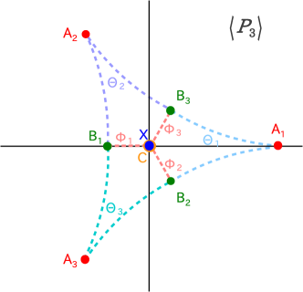
Figure 1: A sketch of the possible values of Polyakov loop in each phase. $(A_{1},A_{2},A_{3})$ and $(B_{1},B_{2},B_{3})$ form ${\rm Z}_{3}$ triplets. $\Theta$ and $\Phi$ are interpolating configurations useful in the description of the mixed fermion content case.

Figure 1 shows all relevant values of $P_{3}$ in the complex plane. $(A_{1},A_{2},A_{3})$ and $(B_{1},B_{2},B_{3})$ form $Z_{3}$ triplets. In lattice simulations one measures both the VEVs and eigenvalue distributions of $P_{3}$ in eq. (16) and $P_{8}$ in eq. (17). The absolute value of $P_{3}$ is strongly affected by quantum fluctuations of $\theta_{H}$ and is reduced at strong gauge couplings. The phase of $P_{3}$, on the other hand, is less affected by quantum fluctuations in the weak coupling regime so that transitions from one phase to another can be seen as changes in the phase of $P_{3}$ and density plots of eigenvalue phases of $P_{3}$. The former has been found in ref. Cossu and D’Elia (2009). The classifications of $A$, $B$ and $C$ are summarized in Table 1, where we also include the confined phase, denoted by $X$, in which $\theta_{H}$ fluctuate and take all possible values, with equal probability.

The $Z_{3}$ center symmetry is yet another global symmetry. If the action has this symmetry as in the pure gauge theory or only with adjoint fermions, then its spontaneous breaking is possible. The magnitude of $P_{3}$ is the order parameter in this case. This symmetry is broken in the $A$-phase and the $B$-phase while it is unbroken in the $C$-phase. The phases can be classified by their global SU(3) and $Z_{3}$ symmetries as follows, $X$: (SU(3) symmetric, $Z_{3}$ symmetric), $A$: (SU(3) symmetric, $Z_{3}$ broken), $B$: (SU(3) broken, $Z_{3}$ broken) and $C$: (SU(3) broken, $Z_{3}$ symmetric).

	$\begin{matrix}\theta_{H}=(\theta_{1},\theta_{2},\theta_{3})\cr\rm and~{}permutations\end{matrix}$	$P_{3}$	$P_{8}$	$\begin{matrix}\rm Global\ Symmetry,\cr\rm Phase\end{matrix}$
$X$	$\begin{matrix}\rm Large~{}quantum\cr\rm fluctuations\end{matrix}$	$0$	$-\frac{1}{8}$	$\begin{matrix}\rm SU(3),\cr\rm confined\end{matrix}$
$\begin{matrix}A_{1}\cr A_{2,3}\end{matrix}$	$\begin{matrix}(0,0,0)\cr(\pm\hbox{$\frac{2}{3}$}\pi,\pm\hbox{$\frac{2}{3}$}\pi,\pm\hbox{$\frac{2}{3}$}\pi)\end{matrix}$	$\begin{matrix}1\cr e^{\pm 2\pi i/3}\end{matrix}$	1	$\begin{matrix}\rm SU(3),\cr{\rm deconfined}\end{matrix}$
$\begin{matrix}B_{1}\cr B_{2,3}\end{matrix}$	$\begin{matrix}(0,\pi,\pi)\cr(\pm\hbox{$\frac{2}{3}$}\pi,\mp\hbox{$\frac{1}{3}$}\pi,\mp\hbox{$\frac{1}{3}$}\pi)\end{matrix}$	$\begin{matrix}-\hbox{$\frac{1}{3}$}\cr\hbox{$\frac{1}{3}$}e^{\mp\pi i/3}\end{matrix}$	0	$\begin{matrix}\rm SU(2)\times U(1),\cr{\rm split}\end{matrix}$
$C$	$(0,\hbox{$\frac{2}{3}$}\pi,-\hbox{$\frac{2}{3}$}\pi)$	0	$-\frac{1}{8}$	$\begin{matrix}\rm U(1)\times U(1),\cr{\rm reconfined}\end{matrix}$

Table 1: Classification of the location of the global minima of $V_{\rm eff}(\theta_{H})$. In the last column the names of the corresponding phases termed in ref. Cossu and D’Elia (2009) are also listed for $X,A,B$ and $C$.

IV Perturbative results

In this section, we present the analysis on the effective potential $V_{\rm eff}(\theta_{H})$ as a function of the AB phase $\theta_{H}$. The location of its global minimum defines the VEVs of $\theta_{H}\ ({\rm mod}\ 2\pi)$. We first give the formula for $V_{\rm eff}(\theta_{H})$ at one-loop level, and then discuss the relationship between $\theta_{H}$ and the Polyakov loops $P_{3}$ and $P_{8}$.

IV.1 One-loop effective potential

The first step is to separate the gauge field $A_{y}$ into its vacuum expectation value $\langle A_{y}\rangle$ and the quantum fluctuation $A_{y}^{q}$. At one-loop level, the effective potential is obtained by the determinant of the logarithm of the quadratic action.

In the background gauge, which is defined by the gauge fixing

$${\cal L}_{\rm gf} = -\frac{1}{2\alpha}{\rm Tr\,}F[A]^{2},$$

$$F[A] = \partial_{\mu}A^{\mu}+ig[\raise 0.68889pt\hbox{$\langle$}\lower 0.68889pt\hbox{}A_{\mu}\raise 0.68889pt\hbox{$\rangle$}\lower 0.68889pt\hbox{},A^{\mu}]$$ (29)

and the gauge parameter $\alpha=1$ (Feynman-’t Hooft gauge), the one-loop effective potential in $R^{d-1}$, after a Wick rotation, is given by

$$V_{\rm eff}^{\rm g+gh}(\theta_{H}) = \frac{d-2}{2\cdot({\rm volume})_{d-1}}\,\ln\det[-D_{\rm g+gh}^{2}]~{},$$

$$V_{\rm eff}^{\rm R}(\theta_{H}) = -\frac{2^{{\lfloor d/2\rfloor}-1}}{({\rm volume})_{d-1}}\,\ln\det[-D_{\rm R}^{2}]~{},$$ (30)

for the contributions coming from gauge and ghost fields and from fermions in the representation ${\rm R}\in\{{\rm fd},{\rm ad}\}$. $({\rm volume})_{d-1}$ denotes the volume of $R^{d-1}$. $d-2$ counts the number of physical degrees of freedom of a gauge boson. $\lfloor d/2\rfloor$ gives the largest integer which is equals to or smaller than $d/2$ and thus $2^{\lfloor d/2\rfloor}$ counts the number of degrees of freedom of a Dirac fermion in $d$-dimensional space-time.

In the background configuration

$$\langle A_{y}\rangle = \frac{1}{2\pi Rg}\,\text{diag}\,(\theta_{1},\theta_{2},\theta_{3}),\quad\sum_{i=1}^{3}\theta_{j}=0~{},$$ (31)

the expressions for $-D_{\rm g+gh}^{2}$, $-D_{\rm fd}^{2}$ and $-D_{\rm ad}^{2}$ are given by

$$[-D_{\rm g+gh}^{2}]_{jk} = -\partial_{\mu}\partial^{\mu}-\left[\partial_{y}+i\left(\frac{\theta_{j}-\theta_{k}}{2\pi R}\right)\right]^{2},$$

$$\left[-D_{\rm fd}^{2}\right]_{j} = -\partial_{\mu}\partial^{\mu}-\left[\partial_{y}+i\left(\frac{\theta_{j}+\alpha_{\rm fd}}{2\pi R}\right)\right]^{2}+m_{\rm fd}^{2}\,,$$

$$\left[-D_{\rm ad}^{2}\right]_{jk} = -\partial_{\mu}\partial^{\mu}-\left[\partial_{y}+i\left(\frac{\theta_{j}-\theta_{k}+\alpha_{\rm ad}}{2\pi R}\right)\right]^{2}+m_{\rm ad}^{2}\,.$$ (32)

Thus the one-loop effective potential becomes

$$V_{\rm eff}(\theta_{H}) = V_{\rm eff}^{\rm g+gh}(\theta_{H})+N_{\rm fd}V_{\rm eff}^{{\rm fd}}(\theta_{H})+N_{\rm ad}V_{\rm eff}^{{\rm ad}}(\theta_{H})~{},$$ (33)

$$V_{\rm eff}^{\rm g+gh}(\theta_{H}) \equiv \frac{d-2}{2}\sum_{j,k=1}^{3}\sum_{n=-\infty}^{\infty}\int\frac{d^{d-1}p}{(2\pi)^{d-1}}\ln[p^{2}+(m_{A}^{(n)})^{2}_{jk}]~{},$$ (34)

$$V_{\rm eff}^{{\rm fd}}(\theta_{H}) \equiv -2^{{\lfloor d/2\rfloor}-1}\sum_{j=1}^{3}\sum_{n=-\infty}^{\infty}\int\frac{d^{d-1}p}{(2\pi)^{d-1}}\ln[p^{2}+(m_{\rm fd}^{(n)})^{2}_{j}]~{},$$ (35)

$$V_{\rm eff}^{\rm ad}(\theta_{H}) \equiv -2^{{\lfloor d/2\rfloor}-1}\sum_{j,k=1}^{3}\sum_{n=-\infty}^{\infty}\int\frac{d^{d-1}p}{(2\pi)^{d-1}}\ln[p^{2}+(m_{\rm ad}^{(n)})^{2}_{jk}]~{},$$ (36)

where $(m_{A}^{(n)})^{2}$, $(m_{\rm fd}^{(n)})^{2}$ and $(m_{\rm ad}^{(n)})^{2}$ are given in (22), and $N_{\rm fd}$ and $N_{\rm ad}$ are the numbers of fermions in the fundamental and adjoint representations, respectively.

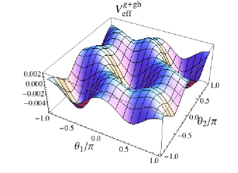
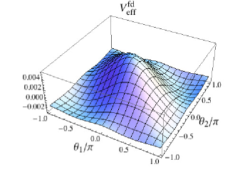
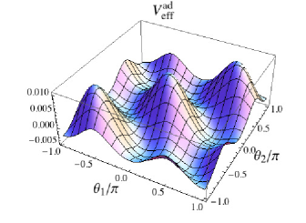
Figure 2: Three contributions to the effective potential $V_{\rm eff}^{\rm g+gh}(\theta_{H})$, $V_{\rm eff}^{\rm ad}(\theta_{H})$ and $V_{\rm eff}^{\rm fd}(\theta_{H})$ are plotted for the case with $d=4$, $m_{\rm fd}=m_{\rm ad}=0$ and $\alpha_{\rm fd}=\alpha_{\rm ad}=0$. $R$ is normalized to unity.

Note that, in eq. (36), both the momentum integrations and the infinite sums of KK modes yield ultraviolet (UV) divergences which are independent of $\theta_{H}$ and $\alpha_{{\rm fd},{\rm ad}}$. Through the calculations summarized in Appendix A, we obtain expressions of each contribution

$$V_{\rm eff}^{\rm g+gh}(\theta_{H}) = (d-2)\sum_{j,k=1}^{3}V(\theta_{j}-\theta_{k},0),$$

$$V_{\rm eff}^{\rm fd}(\theta_{H}) = -2^{\lfloor d/2\rfloor}\sum_{j=1}^{3}V(\theta_{j}+\alpha_{\rm fd},m_{\rm fd}),$$

$$V_{\rm eff}^{\rm ad}(\theta_{H}) = -2^{\lfloor d/2\rfloor}\sum_{j,k=1}^{3}V(\theta_{j}-\theta_{k}+\alpha_{\rm ad},m_{\rm ad}),$$ (37)

where

$$V(\theta,m) = \frac{\Gamma(d/2)}{\pi^{d/2}(2\pi R)^{d-1}}h_{d}(\theta,m)~{},$$ (38)

$$h_{d}(\theta,m) = \sum_{k=1}^{\infty}\frac{1-\cos k\theta}{k^{d}}B_{d/2}(2\pi kmR)~{},$$ (39)

$$B_{d/2}(x) \equiv \frac{x^{d/2}K_{d/2}(x)}{2^{\frac{d}{2}-1}\Gamma(d/2)},\quad B_{d/2}(0)=1,$$ (40)

and $K_{d/2}(x)$ is the modified Bessel function of the second kind.

In Fig. 2, $V_{{\rm eff}}^{\rm g+gh}(\theta_{H})$, $V_{{\rm eff}}^{\rm ad}(\theta_{H})$ and $V_{{\rm eff}}^{\rm fd}(\theta_{H})$ are plotted for $m_{\rm fd}=m_{\rm ad}=0$ and $\alpha_{\rm ad}=\alpha_{\rm fd}=0$. In this case, $V_{{\rm eff}}^{\rm g+gh}(\theta_{H})$ has degenerate global minima at $A_{1,2,3}$, reflecting the $Z_{3}$ symmetry. On the other hand, $V_{{\rm eff}}^{\rm fd}(\theta_{H})$ has degenerate global minima at $A_{2}$ and $A_{3}$ while $V_{{\rm eff}}^{\rm ad}(\theta_{H})$ has global minima at $C$, i.e. at the all permutations of $(0,\hbox{$\frac{2}{3}$}\pi,-\hbox{$\frac{2}{3}$}\pi)$.

In the case with adjoint fermion and $\alpha_{\rm ad}=0$, the effective potential can be rewritten, neglecting terms independent of $\theta_{H}$, in terms of the trace of $W_{3}^{k}$ in eq. (10) giving:

$$\sum_{i,j}^{3}h_{d}(\theta_{i}-\theta_{j},m)\propto-\sum_{k=1}^{\infty}\frac{|{\rm Tr\,}W_{3}^{k}|^{2}}{k^{d}}B_{d/2}(2\pi kmR)\equiv-\sum_{k=1}^{\infty}c_{k}(mR)|{\rm Tr\,}W_{3}^{k}|^{2}$$ (41)

which gives a direct interpretation as the sum of contributions coming from paths wrapping $k$ times in the compact direction (see also Anber and Unsal (2013)). The sum is dominated by the first term ($k=1$) for every values of $mR$ (the worst case being $mR=0$ where $c_{1}/c_{2}=2^{d}$), and it looks like a self interaction of the Polyakov loop, respecting the center symmetry. Indeed, terms like this appear in various dimensionally reduced models with center stabilization terms, and are known as double-trace deformations (see e.g. Ogilvie (2012)). In the limit $mR\rightarrow 0$ (i.e. $c_{1}\rightarrow 1$), the combined potential of gluons and adjoint fermions has the minimum for $|P_{3}|=0$ (a phase with confinement) as we show in the next section. The opposite limit $mR\rightarrow\infty$ corresponds to the pure gauge case, $c_{1}\rightarrow 0$. We use these observations later in the discussion on the phase diagram found on the lattice.

IV.2 Vacuum in presence of fermions

In the presence of fermions, $V_{\rm eff}(\theta_{H})$ exhibits a rich structure. Let us consider a model with $N_{\rm fd}$($N_{\rm ad}$) fundamental (adjoint) fermions which is described by eq. (33). For simplicity, we restrict ourselves to the case where $m_{\rm fd}=m_{\rm ad}$ and $\alpha_{\rm fd}=\alpha_{\rm ad}$. $N_{\rm fd}=4$ and $N_{\rm ad}=2$ are the minimal numbers of flavors for the standard staggered formalism for the lattice fermion used in the simulations. Therefore, in the following we briefly summarize the behavior of $V_{{\rm eff}}(\theta_{H})$ for $(N_{\rm fd},N_{\rm ad})=(0,2)$ and $(4,0)$ for $d=4$, i.e. $R^{3}\times S^{1}$ compactification.

IV.2.1 Adjoint fermions : $(N_{\rm fd},N_{\rm ad})=(0,2)$

Let us begin with the case of adjoint fermions under the periodic boundary condition $\alpha_{\rm ad}=0$. At one-loop level, $V_{\rm eff}(\theta_{H})$ depends on the mass in the product $m_{\rm ad}R$. The global minimum of $V_{\rm eff}(\theta_{H})$ changes position according to the following pattern:

$$A_{1,2,3}\ \ {\rm for} \ \ 0.499\leq m_{\rm ad}R~{},$$

$$B_{1,2,3}\ \ {\rm for} \ \ 0.421\leq m_{\rm ad}R\leq 0.499~{},$$

$$C\ \ {\rm for} \ \ 0\leq m_{\rm ad}R\leq 0.421~{}.$$ (42)

The fact that there are coexisting phases $A$ and $B$ ($B$ and $C$) at the transition point $m_{\rm ad}R=0.421(0.499)$ implies that the transition is of first order.

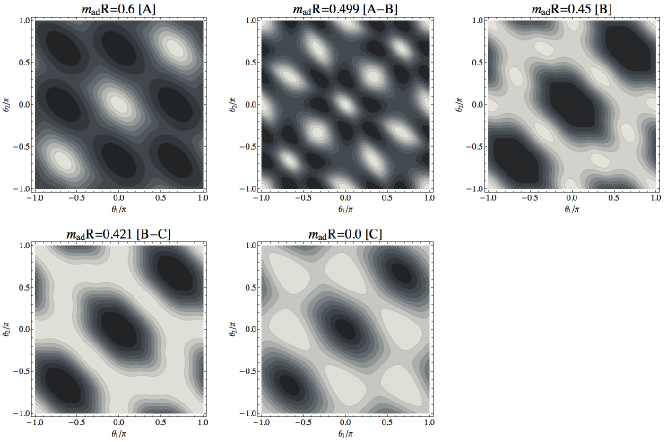
Figure 3: Effective potential for the case of $N_{\rm ad}=2$ adjoint fermion with periodic boundary condition ($\alpha_{\rm ad}=0$) for the values of $m_{\rm ad}R$ in $d=4$. They are corresponding to the $A$ phase, the $A$-$B$ transition point, the $B$ phase, the $B$-$C$ transition point and the $C$ phase, respectively. Lower values of $V_{{\rm eff}}$ are indicated by lighter colors.

In Fig. 3, contour plots of $V_{\rm eff}(\theta_{H})$ are displayed in the order $m_{\rm ad}R$ is decreasing to cover the phases $A$, $B$ and $C$ and transitions $A$-$B$ and $B$-$C$ according to eq. (42). One notes that the $A$-$B$ transition is more prominent than the $B$-$C$ transition because the barrier separating two minima in the potential is much higher for the former.

We find that the location of the global minimum depends on the value of $\alpha_{\rm ad}$ as well. In particular, for $\alpha_{\rm ad}=\pi$, the effective potential is identical to that at finite temperature $T=(2\pi R)^{-1}$ and the SU(3) symmetry remains unbroken. For massless fermions $m_{\rm ad}=0$, the global minima of the effective potential are located at

$$A_{1,2,3}\ \ {\rm for}\ \ 0.416\pi\leq|\alpha_{\rm ad}|\leq\pi~{},$$

$$B_{1,2,3}\ \ {\rm for}\ \ 0.319\pi\leq|\alpha_{\rm ad}|\leq 0.416\pi~{},$$

$$C\ \ {\rm for}\ \ |\alpha_{\rm ad}|\leq 0.319\pi~{}.$$ (43)

IV.2.2 Fundamental fermions : $(N_{\rm fd},N_{\rm ad})=(4,0)$

In the presence of the fundamental fermions, the global $Z_{3}$ symmetry

$$\theta_{j}\to\theta_{j}+\frac{2}{3}\pi~{},\quad j=1,2,3.$$ (44)

is broken. The boundary condition parameter $\alpha_{\rm fd}$ plays the role of selecting one of the $Z_{3}$ related minima. We find that the fermion mass $m_{\rm fd}$, on the other hand, has only a small effect on the location of the global minimum unless $m_{\rm fd}R$ is large enough for the effect of fermions to be negligible. Contour plots of $V_{\rm eff}(\theta_{H})$ with $d=4$ and $N_{\rm fd}=4$ are displayed for various values of $\alpha_{\rm fd}$ in Fig. 4.

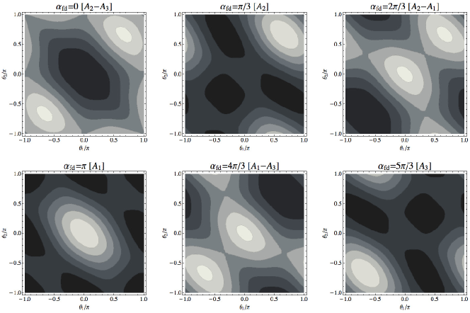
Figure 4: The effective potential with four massless fundamental fermions in the $(\theta_{1}/\pi,\theta_{2}/\pi)$ plane. Boundary condition of the fermions are changed from $\alpha_{\rm fd}=0$ to $\alpha_{\rm fd}=5\pi/3$. We plot the three phase transitions $A_{2}$-$A_{3}$, $A_{2}$-$A_{1}$ and $A_{1}$-$A_{3}$, and three phases $A_{1}$, $A_{2}$ and $A_{3}$. Lower values of $V_{{\rm eff}}$ are indicated by lighter colors.

The global minimum is found at

$$A_{2}\ \ {\rm for}\ \ 0\leq\alpha_{\rm fd}\leq\frac{2\pi}{3}~{},$$

$$A_{1}\ \ {\rm for}\ \ \frac{2\pi}{3}\leq\alpha_{\rm fd}\leq\frac{4\pi}{3}~{},$$

$$A_{3}\ \ {\rm for}\ \ \frac{4\pi}{3}\leq\alpha_{\rm fd}\leq 2\pi~{}.$$ (45)

Therefore, the phase changes $A_{2}\rightarrow A_{1}\rightarrow A_{3}\rightarrow A_{2}$ as $\alpha_{\rm fd}$ increases from $0$ to $2\pi$. In Fig. 5, we plot the corresponding $V_{{\rm eff}}(\theta_{H})$ a function of $\alpha_{\rm fd}$ for two different values of $m_{\rm fd}R$. One observes that the line of global minima has a period of $2\pi/3$ and non-analyticity at $\alpha_{\rm fd}=2n\pi/3,\ \ (n=0,1,2,\dots)$, and the transition is expected to be of first order. This is known as Roberge-Weiss phase structure Roberge and Weiss (1986) which we discuss in Sec. V.3.

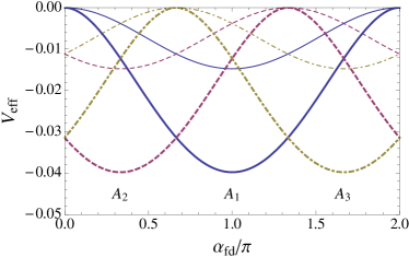
Figure 5: $V_{{\rm eff}}$ for $(N_{\rm fd},N_{\rm ad})=(4,0)$ versus $\alpha_{\rm fd}$. Solid, dashed and dot-dashed lines correspond to values at $A_{1}$, $A_{2}$ and $A_{3}$, respectively. Thick [thin] lines are for $m_{\rm fd}=0$ [$m_{\rm fd}R=0.4$].

IV.3 Scalar (Higgs) masses

As discussed in Sec. III, non-vanishing $\theta_{j}$ in (31) can induce symmetry breaking where zero modes $\phi(x)\equiv A_{y}^{(0)}(x)$ play the role of the Higgs field in $R^{d-1}$. With the normalization in eq. (19), $-\int dy\,{\rm Tr}\,F_{\mu y}^{2}$ yields the canonically normalized kinetic term for $\phi(x)$. There are eight real scalars; $\phi(x)=\sum_{a=1}^{8}\phi_{a}(x)T^{a}$ where $T^{a}$’s are $SU(3)$ generators. Some of them are absorbed by $A_{\mu}^{(0)}(x)$, which makes vector fields massive in the broken symmetry sector. The rest of the $\phi_{a}$’s remain physical. They are massless at the tree level, but acquire finite masses at the quantum level. In the application to electroweak interactions, they correspond to the physical neutral Higgs boson.

The masses of these physical scalar fields are related to $V_{\rm eff}(\theta_{1},\theta_{2})$ in the previous subsections. $V_{\rm eff}(\theta_{1},\theta_{2})$ is the effective potential for $\phi_{3}(x)$ and $\phi_{8}(x)$ as well. The relationship between $\{\theta_{j}\}$ and $\{\phi_{a}\}$ are given by

$$(\theta_{1},\theta_{2},\theta_{3})=g\sqrt{\frac{\pi R}{2}}~{}\bigg{(}\phi_{3}+\frac{\phi_{8}}{\sqrt{3}},-\phi_{3}+\frac{\phi_{8}}{\sqrt{3}},-\frac{2}{\sqrt{3}}\phi_{8}\bigg{)}~{}.$$ (46)

The mass eigenstates are determined by diagonalizing the mass matrix $\partial^{2}V_{\rm eff}/\partial\phi_{a}\partial\phi_{b}$ $(a,b=3,8)$ at the minimum of $V_{\rm eff}$. One easily finds $\phi_{3}$ and $\phi_{8}$ are the eigenstates whose masses are given by

$$m_{3}^{2} = \frac{g^{2}\pi R}{2}\Big{(}\frac{\partial}{\partial\theta_{1}}-\frac{\partial}{\partial\theta_{2}}\Big{)}^{2}~{}V_{\rm eff}(\theta_{1},\theta_{2})\Big{|}_{\rm min}~{},$$ (47)

$$m_{8}^{2} = \frac{g^{2}\pi R}{6}\Big{(}\frac{\partial}{\partial\theta_{1}}+\frac{\partial}{\partial\theta_{2}}\Big{)}^{2}~{}V_{\rm eff}(\theta_{1},\theta_{2})\Big{|}_{\rm min}$$ (48)

where the second derivatives are evaluated at the global minimum of $V_{\rm eff}$. Note that although the form of the effective potential $V_{\rm eff}(\phi_{a})$ is gauge-dependent in general, the masses of the scalar fields $\phi_{a}$, which are related to the curvatures of $V_{\rm eff}$ at its global minimum, are gauge-invariant quantities. In particular, the expression (48) is valid to $O(g^{2})$.

At this stage it is instructive to see how the formulas would change or remain invariant when a different boundary condition were adopted. Suppose that the boundary condition matrix $V$ in (2) is given by

$$V=\begin{pmatrix}e^{i\delta_{1}}\cr&e^{i\delta_{2}}\cr&&e^{i\delta_{3}}\end{pmatrix},\quad\sum_{j=1}^{3}\delta_{j}=0~{}.$$ (49)

With this boundary condition the spectra of the KK modes of $A_{M},\psi_{\rm fd},\psi_{\rm ad}$ are given by the formula (22) where $\theta_{j}$ is replaced by $\theta_{j}-\delta_{j}$. As a consequence the effective potential is given by

$$V_{\rm eff}(\theta_{1},\theta_{2};\delta_{1},\delta_{2})=V_{\rm eff}(\theta_{1}-\delta_{1},\theta_{2}-\delta_{2};0,0)~{},$$ (50)

where $V_{\rm eff}(\theta_{1}-\delta_{1},\theta_{2}-\delta_{2};0,0)$ is $V_{\rm eff}(\theta_{1},\theta_{2})$ given by (33) and (37). The location of the global minimum of $V_{\rm eff}$ is given by $\theta_{j}^{\rm min}(\delta_{1},\delta_{2})=\theta_{j}^{\rm min}(0,0)+\delta_{j}$. The masses $m_{3}$ and $m_{8}$ in (48) remain invariant.

As an example, consider the case with $d=4,N_{\rm fd}=0,\alpha_{\rm ad}=0$. The effective potential is given by

$$V_{\rm eff}(\theta_{1},\theta_{2}) = \frac{1}{2\pi^{5}R^{3}}\Big{[}h_{4}(\theta_{1}-\theta_{2},0)+h_{4}(2\theta_{1}+\theta_{2},0)+h_{4}(\theta_{1}+2\theta_{2},0)$$ (52)

$$\hskip-14.22636pt-2N_{\rm ad}\big{\{}h_{4}(\theta_{1}-\theta_{2},m_{\rm ad})+h_{4}(2\theta_{1}+\theta_{2},m_{\rm ad})+h_{4}(\theta_{1}+2\theta_{2},m_{\rm ad})\big{\}}\Big{]}~{}.$$

Here $h_{4}(\theta,m)$ is defined in (40). The masses are given by

$$m_{3}^{2} = \frac{g^{2}}{4\pi^{4}R^{2}}\Big{[}\big{\{}4h_{4}^{(2)}(\theta_{1}-\theta_{2},0)+h_{4}^{(2)}(2\theta_{1}+\theta_{2},0)+h_{4}^{(2)}(\theta_{1}+2\theta_{2},0)\big{\}}$$ (54)

$$-2N_{\rm ad}\big{\{}4h_{4}^{(2)}(\theta_{1}-\theta_{2},m_{\rm ad})+h_{4}^{(2)}(2\theta_{1}+\theta_{2},m_{\rm ad})+h_{4}^{(2)}(\theta_{1}+2\theta_{2},m_{\rm ad})\big{\}}\Big{]}_{\rm min}~{},$$

$$m_{8}^{2} = \frac{3g^{2}}{4\pi^{4}R^{2}}\Big{[}\big{\{}h_{4}^{(2)}(2\theta_{1}+\theta_{2},0)+h_{4}^{(2)}(\theta_{1}+2\theta_{2},0)\big{\}}$$ (56)

$$\hskip 28.45274pt-2N_{\rm ad}\big{\{}h_{4}^{(2)}(2\theta_{1}+\theta_{2},m_{\rm ad})+h_{4}^{(2)}(\theta_{1}+2\theta_{2},m_{\rm ad})\big{\}}\Big{]}_{\rm min}~{},$$

where $h_{4}^{(2)}(\theta,m)=d^{2}h_{4}(\theta,m)/d\theta^{2}$.

The corresponding mass spectrum for each phase is as follows.

A: SU(3) symmetric

In this phase all $\phi_{a}$ are physical, and all $m_{a}$’s are degenerate.

$$m_{a}^{2}=\frac{3g^{2}}{2\pi^{4}R^{2}}\big{\{}h_{4}^{(2)}(0,0)-2N_{\rm ad}h_{4}^{(2)}(0,m_{\rm ad})\big{\}}\quad(a=1,\cdots,8)~{}.$$ (57)

B: SU(2) $\times$ U(1) symmetric

In this phase $\phi_{4},\phi_{5},\phi_{6},\phi_{7}$ are absorbed by the corresponding vector fields. $\phi_{1},\phi_{2},\phi_{3},\phi_{8}$ are physical.

$$m_{1}^{2} =m_{2}^{2}=m_{3}^{2}$$ (59)

$$=\frac{g^{2}}{2\pi^{4}R^{2}}\Big{[}2h_{4}^{(2)}(0,0)+h_{4}^{(2)}(\pi,0)-2N_{\rm ad}\big{\{}2h_{4}^{(2)}(0,m_{\rm ad})+h_{4}^{(2)}(\pi,m_{\rm ad})\big{\}}\Big{]}~{},$$

$$m_{8}^{2} =\frac{3g^{2}}{2\pi^{4}R^{2}}\Big{[}h_{4}^{(2)}(\pi,0)-2N_{\rm ad}h_{4}^{(2)}(\pi,m_{\rm ad})\Big{]}~{}.$$ (60)

Notice that $m_{1,2,3}\not=m_{8}$.

C: U(1) $\times$ U(1) symmetric

In this phase $\phi_{1},\phi_{2},\phi_{4},\phi_{5},\phi_{6},\phi_{7}$ are absorbed by the corresponding vector fields. $\phi_{3},\phi_{8}$ are physical.

$$m_{3}^{2}=m_{8}^{2}=\frac{3g^{2}}{2\pi^{4}R^{2}}\Big{[}h_{4}^{(2)}(\hbox{$\frac{2}{3}$}\pi,0)-2N_{\rm ad}h_{4}^{(2)}(\hbox{$\frac{2}{3}$}\pi,m_{\rm ad})\Big{]}~{}.$$ (61)

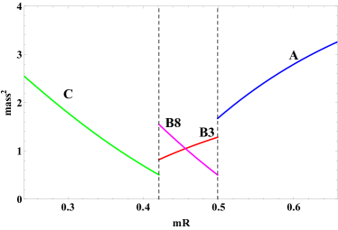
Figure 6: The dependence on the compactification parameter $mR$ of scalar “Higgs” mass squared in phases A, B and C for $(N_{\rm fd},N_{\rm ad})=(0,2)$. For each phase, the value in units of $g^{2}/2\pi^{4}R^{2}$ is plotted. B3 and B8 are the masses for the $m_{3}^{2}$ and $m_{8}^{2}$ in eq. (60), respectively.

In Fig. 6 we plot the dependence of the masses on the parameter $mR$ in the A, B and C phases. We note here that $m_{3}$ and $m_{8}$ are expected to cross at some value of $mR\sim 0.46$ in the B phase and that $m_{3}=m_{8}$ in the C-phase grows as $mR\rightarrow 0$ (i.e. $\beta\rightarrow\infty$ in terms of lattice parameters).

V Lattice results

Following the general remarks in Sec. V.1, we present our lattice study with the adjoint (fundamental) fermions in Secs. V.2 (V.3). We separately discuss, in Sec. V.2.2, the connection to the perturbative prediction by the analysis of the eigenvalue distribution.

V.1 General remarks

The lattice action used through the entire work is the standard Wilson gauge action and standard staggered fermions (in the fundamental and adjoint representation).

We compute Polyakov loops $P_{3}$ and $P_{8}$ on the $16^{3}\times 4$ volume gauge configurations sampled with the weight $e^{-S_{g}-S_{f}}$, where the lattice actions $S_{g}$ and $S_{f}$ are given in eqs. (13) and (14), respectively. By comparing the distribution of $P_{3}$ on the complex plane and Fig. 1, one can distinguish which phase is realized. This qualitative analysis is also done in comparing the eigenvalue distribution and the vacua (Figs. 3 and 5) obtained from the perturbative analysis. The transition points are determined by the susceptibility

$$\chi_{\Omega}=N_{x}^{3}\left(\langle\Omega^{2}\rangle-\langle\Omega\rangle^{2}\right)$$ (62)

of the observable $\Omega\in\{|P_{3}|,P_{8}\}$ which should scale with the lattice volume for first order phase transitions. In connection to the perturbative results, where the relevant parameter is $m_{\rm fd}R$ or $m_{\rm ad}R$, increasing $\beta$ has the effect of decreasing those parameters, due to the running of the renormalized fermion mass in the lattice unit. We estimate statistical errors by employing the jackknife method with appropriate bin sizes to incorporate any auto-correlations.

V.2 Adjoint fermions

V.2.1 Phase structure

In the numerical simulation for $(N_{\rm ad},N_{\rm fd})=(2,0)$, we use bare masses $m_{\rm ad}a=ma=0.05$ and 0.10, changing $\beta$ covering the range $5.3\leq\beta\leq 6.5$. Periodic boundary condition is used ($\alpha_{\rm ad}=0$) in the compact direction, which is different from the case with anti-periodic boundary conditions (finite temperature) where only the confined and deconfined phases are realized Karsch and Lutgemeier (1999). To explore the phase structure in heavier mass region, we also examine bare masses $m_{\rm ad}a=ma=0.50$ and $0.80$ for the range of $5.5\leq\beta\leq 9.8$ and $5.5\leq\beta\leq 20.0$, respectively. As will be discussed, data with those masses require even more careful treatment.

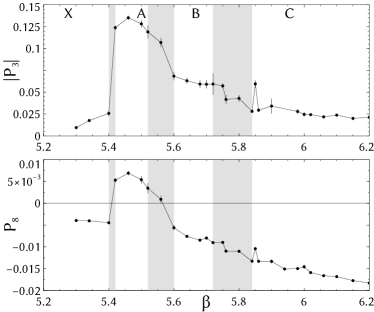
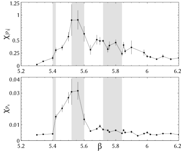
Figure 7: Left: $\beta$-dependences of $|P_{3}|$ (upper) and $P_{8}$ (lower). The gray bands indicate the transition regions as listed in Table 2. Each phase is labeled in the upper panel, accordingly. Right: susceptibilities corresponding to the light panels. Results for $ma=0.05$ are shown.

For each $ma$, after checking rough phase structure from the distribution plot of $P_{3}$, we determine the transition points which we call $\beta_{X/A}$, $\beta_{A/B}$ and $\beta_{B/C}$ for the $X$-$A$, $A$-$B$ and $B$-$C$ transitions, respectively (see Figs. 7, 8, 9 and 10). For this purpose, it is convenient to investigate $|P_{3}|$, $P_{8}$ and the susceptibilities of them. Since the data is at finite physical volume, and the $P$ are not renormalized, their magnitudes could differ from the predictions summarized in Table 1. Nevertheless, from the $|P_{3}|$ data, we can identify four regions for all the masses studied, that respectively correspond to the observation of phases $X$, $A$, $B$ and $C$. The peaks of the susceptibility at the $B$-$C$ transition is milder than the first two as explained in the qualitative discussion of potential barrier in Sec. IV.2.1 for the behavior of $V_{{\rm eff}}(\theta_{H})$. It is also interesting to see that $P_{8}$ becomes zero at the $X$-$A$ transition ($\beta=5.42$) and the $A$-$B$ transition ($\beta=5.70$). The values at these points change from $-1/8$ to $1$ and from $1$ to $0$ according to the analytical prediction summarized in Table 1. Since, in general, the change of the sign in observables is not affected by lattice artifacts, the zeros of $P_{8}$ give a reliable way of locating the transition points. However, this idea is only applicable to the transition where the sign of $P_{8}$ changes. Contrary to the analytic prediction, $P_{8}$ takes a negative value in the $B$-phase for reasons which we will discuss later. Therefore, there is no possibility to have another zero around $\beta=6.0$ for the $B$-$C$ transition. As seen in the figure, $\chi_{P_{8}}$ is less sensitive to the transitions than others, hence remains in a complemental role.

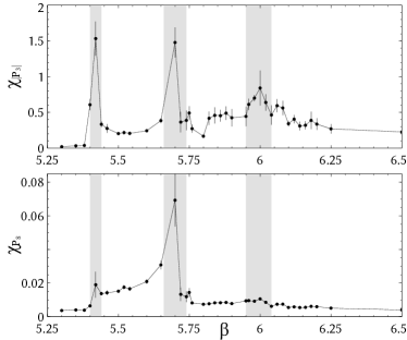
Figure 8: Same figure as Fig. 8 but for $ma=0.10$.

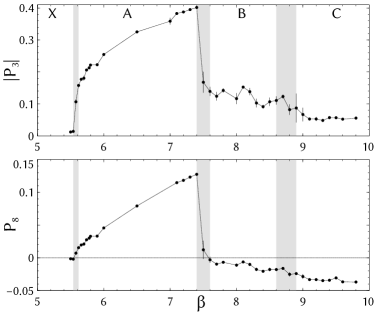
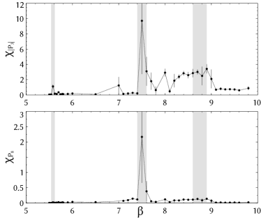
Figure 9: Same figure as Fig. 8 but for $ma=0.50$.

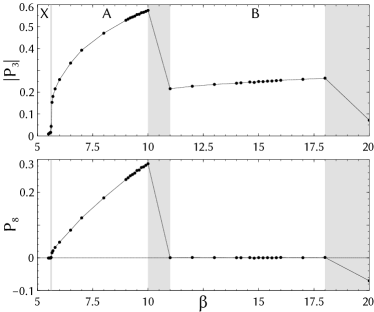
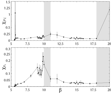
Figure 10: Same figure as Fig. 8 but for $ma=0.80$.

Looking over $P_{8}$ for all bare masses, we see the $X$-$A$ transition point depends on $ma$ only mildly. This is explained by the fact that the existence of the adjoint fermions does not affect the ${\rm Z}_{3}$ symmetry because the adjoint gauge link is invariant under the associated global ${\rm Z}_{3}$ transformation. On the other hand, for larger $ma$, the $A$-$B$ transition occurs at the larger $\beta$ at which, in the perturbative language, the value of $m_{\rm ad}R=\hat{m}(\beta)\times N_{y}/2\pi$ remains in the same level by the running of the renormalized mass $\hat{m}(\beta)$ in the lattice unit. Accordingly, $P_{8}$ in the $B$-phase approaches zero as expected analytically for the perturbative region. In particular, at $ma=0.80$, $P_{8}$ is consistent with zero in the $B$-phase and the $B$-$C$ transition is detected at the point where $P_{8}$ starts to deviate from zero. However, for such large $\beta$ value, the physical lattice size is exponentially small. For further discussion on the properties of these transitions, a more detailed study on the finite size scaling has to be done.

With a caveat for the heavy mass region, we summarize the critical values of $\beta$ for each mass in Table 2. Based on this result, the phase diagram on the $\beta$-$ma$ plane is depicted in Fig. 11. In the magnified plot in the inset, we show the approach of the $X$-$A$ transition point to the confined-deconfined transition transition point $\beta=5.692(20)$ (dashed line) for the pure gauge case Fukugita et al. (1989). Because the $B$-$C$ transitions are hard to observe clearly from the Polyakov loops or the susceptibilities at this volume, we estimate the interval where the transition occurs as follows. The lower boundary of the interval is the highest $\beta$ where, by inspecting the eigenvalue distribution, we can still clearly identify the $B$-phase. The upper boundary comes accordingly from the lowest $\beta$ where we are certainly in the $C$-phase. Due to the subjective character of the data, we do not quote any error: it is an identification of the region where the transition is occurring.

Table 2: Critical values of $\beta$ for each $ma$.

$ma$	$\beta_{X/A}$	$\beta_{A/B}$	$\beta_{B/C}$
0.05	5.41(1)	5.56(4)	[5.72,  5.84 ]
0.10	5.42(2)	5.70(4)	[5.95,  6.04 ]
0.50	5.58(4)	7.50(10)	[8.60,  8.90 ]
0.80	5.62(4)	10.50(50)	[18.00, 20.00 ]

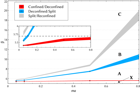
Figure 11: Phase diagram for the $N_{\rm ad}=2$ adjoint fermion system with periodic boundary condition in the compact dimension. In the window, the $X$-$A$ transition line is compared with the pure gauge case (dashed line) Fukugita et al. (1989).

The phase diagram depicted in Fig. 11 can be compared with the perturbative expectations in Sec. IV.2. First we consider “trajectories” with constant $\beta$ on which only the adjoint quark masses change. If the perturbative parameter $m_{\rm ad}$ and the lattice parameter $ma$ are related by a multiplicative factor, which only depends on $\beta$, then we can compare the ratio $m_{\rm A/B}/m_{\rm B/C}$ of these bare parameters at the phase transitions to the prediction from eq. (42) i.e. $\sim 1.18$ (constant). In Fig. 12 we plot the result of this analysis. The intercepts of the constant $\beta$ lines to the phase transition ones are obtained after spline interpolation. The errors are pure statistical not including the systematic of the interpolation method. For $\beta\gtrsim 8$, the lattice results seem to reach a constant value which is $\approx 10\%$ larger than the perturbative one.

It should be noted that since the effective potential is written in terms of ${\rm Tr\,}W_{3}$ in eq. (41) and, as already explained, can be approximated by its first term, our model is then related to a simpler one with the A, B and C phases Bialas et al. (2005); Ogilvie (2012); Myers and Ogilvie (2008). By this comparison, it is inferred that the truncation of the adjoint fermion part to the first term in eq. (41) is enough to reproduce the phase structure.

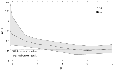
Figure 12: The ratio of mass-parameter at the phase transitions compared with the perturbative prediction. Measurements are done in steps of 0.5 in $\beta$.

V.2.2 Eigenvalues of the Wilson line

The measured values of $P_{3}$ and $P_{8}$ are comparable with the predictions for the Hosotani mechanism listed in Table 1. In order to further clarify the connection of these phases with the perturbative effective potential predictions of Sec. IV.2.1, we present here the main result of the paper: the density plots for the eigenvalues of the Wilson line wrapping around the compact dimension (cf. eq. (4)). These observables are the fundamental degrees of freedom in the perturbative description. We demonstrate also that the lattice non-perturbative calculation matches the perturbative results in the weak coupling limit. In the strong coupling region, we show qualitative agreement with the $V_{\rm eff}$ and its phase structure.

We recall here that on the lattice the Wilson lines are given by

$$W_{3}^{\rm latt}(x)=\prod_{y=1}^{N_{y}}U_{(x,y),4},\ \ W_{8}^{\rm latt}(x)=\prod_{y=1}^{N_{y}}U^{(8)}_{(x,y),4}.$$ (63)

The eigenvalues of the Wilson line, eq. (6), are independent of the gauge transformations, and their degeneracies classify the pattern of gauge symmetry breaking as explained in Sec. III. The three complex eigenvalues are denoted by $\lambda=e^{i\theta_{1}},e^{i\theta_{2}}$ and $e^{i\theta_{3}}$. We constrain each phase within the interval $-\pi\leq\theta_{1},\theta_{2},\theta_{3}\leq\pi$.

A direct comparison of the density plots of the Polyakov loop with the perturbative result for $V_{\rm eff}$ must take into account that a complete degeneracy for the eigenvalues can be never measured directly. This is easily explained by the Haar measure for SU(3) (that can be derived using the Weyl integration formula, see e.g. Simon (1995))

$$\prod_{i>j}\sin^{2}\frac{\theta_{i}-\theta_{j}}{2}=\prod_{i>j}\frac{1}{4}|e^{i\theta_{i}}-e^{i\theta_{j}}|^{2}$$ (64)

which forbids such configurations. See the density plot in Fig. 13, where the eigenvalue triplets of the Polyakov loop is obtained by random numbers constrained by eq. (64). This measure term gives a strong repulsive force for the eigenvalues that must be subtracted to get the non-perturbative $V_{\rm eff}$.

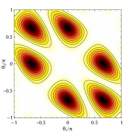
Figure 13: Haar measure density plot. Darker colors denote the highest density regions.

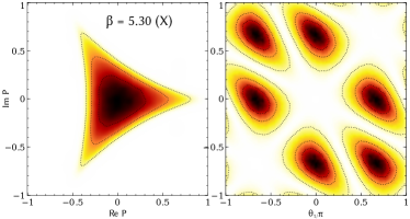
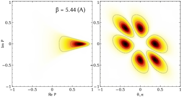
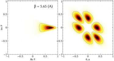
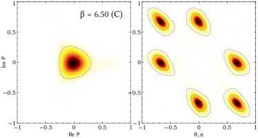
Figure 14: Density plots of the Polyakov loop (in the complex plane) and its eigenvalues (in the $\theta_{1}/\pi$ - $\theta_{2}/\pi$ plane) are shown side-by-side at several $\beta$’s. All possible pairs $\{(\theta_{i},\theta_{j}),i\neq j\}$ are included in the plots. Darker colors denote the highest density regions.

The results of our investigations are shown in the panels of Fig. 14. These plots come in couples and each one of them displays the density plots for the Polyakov loop $P_{3}$ itself (left) and for the phases $(\theta_{1},\theta_{2})$ of its eigenvalues (right). Smearing is applied to the configuration before measurements (5 steps of stout smearing Morningstar and Peardon (2004) with the smearing parameter $\rho=0.2$) to filter the ultraviolet modes that are essentially just lattice noise and are not relevant for $V_{\rm eff}$. By this technique, the gauge configuration is smoothed out by averaging the links over the nearest-neighbors, in a gauge invariant way. Several successive steps of smearing can be applied gradually increasing the radius of involved neighbors. The final result is a configuration where the ultraviolet oscillations of the gauge field at the level of the lattice spacing are highly suppressed. It is typically used to clear propagator signals, or obtain information on topological objects. Since we are only interested in locating the minima of the potential, any fluctuations of the Polyakov loop induced by the coarseness of the lattice around that minima are not relevant at this level. We find that smearing is essential to extract useful information from the configurations generated. Data for the 2D density plots are also smoothed by a gaussian filter with a radius of 5 nearest-neighbors for clarity in the presentation. The panels in Fig. 14, from left to right, top to bottom, show the change of distributions in passing the $X$-$A$-$B$-$C$ phases. Modulo the Haar measure contribution, we observe a good correspondence between the perturbative shape of the potential and the location of the maximum of the densities of the measured Polyakov loop eigenvalues.

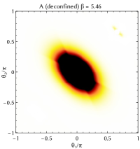
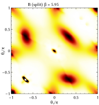
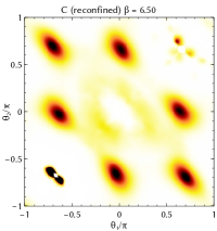
Figure 15: Density plots at several $\beta$’s for the Polyakov Loop eigenvalues (in the $\theta_{1}/\pi$ - $\theta_{2}/\pi$ plane), as in Fig. 14. Here the original data is divided by a similar density plot of the Haar measure distribution. From left to right, the panels correspond to the $X$, $A$, $B$ and $C$ phases. The first panel is white as a result of the calculation. Darker colors denote the highest density regions.

To strengthen our view, we perform another analysis to eliminate the contribution of the Haar measure seen in Fig. 13 from the density plots. We generated a random ensemble of O($5\cdot 10^{6}$) eigenvalues distributed according to the Haar measure (Fig. 13) and, using the same normalization as the lattice data plots of Fig. 14, it is now easy to isolate the effective potential contribution from the kinetic term of the group measure. The result is plotted in Fig. 15. The two-dimensional bins of the histogram have always a finite density of eigenvalues, somewhere very small, so that we are never dividing by zero. Although the procedure introduces some artifacts and more noise due to the subtle cancellations caused by the Haar measure , it is useful from the qualitative point of view. At this stage of the work we would like to show that the effective potential has the features anticipated by the perturbative calculation and can be compared with Fig. 3. Notice that the density plots derived in this way are proportional to $e^{-\int d^{3}x\,V_{\rm eff}}$. Location of the minima (maxima of density) is clearly not affected by this monotonic transformation. The plots, from left to right, are respectively the $X$, $A$, $B$, and $C$ phases ($\beta=5.30,5.46,5.95$ and $6.50$). The distribution in the $X$ (confined) phase is almost a constant i.e. unity so the plot is a white image, which is a manifestation of a uniform random distribution of the eigenvalues in the two dimensional plane. The $A$ and $B$ phases confirm the conjecture of Fig. 14, i.e. that the discrepancy with perturbative prediction is only due to the Haar measure contribution. In the region around $\theta_{1}=\theta_{2}=(0,2\pi/3,-2\pi/3)$, the Haar measure density is close to zero in a wide area and very precise lattice data is needed in order to have a perfect cancellation, sampling also the low density regions, so we see some artifacts as a result. As a further remark we underline that the $C$ phase shows a completely different behavior from the confined one although the Polyakov loop is centered around zero. The eigenvalues are now not distributed in a random fashion but located in peaks around the $Z_{3}$ symmetric values $\theta_{H}=(0,2\pi/3,-2\pi/3)$ (again some artifacts appear), with maximal repulsion between them. There have been recently studies Poppitz et al. (2013); Anber and Unsal (2013) using semi-classical models that relate this phase to a weak coupling region where confinement is realized by abelian degrees of freedom ($U(1)\times U(1)$ remaining). Future works will be devoted to the quantitative tests of these ideas. In conclusion, by removing the gauge group kinetic term from our data, although at the price of introducing some noise, we are able to confirm the nice agreement of lattice data with the perturbative potential. All the four predicted phases are clearly reproduced by the data, which is a strong indication of the realization of the Hosotani mechanism in 3+1 dimensions even at the non-perturbative level. For further confirmation of the Hosotani mechanism on the lattice we need a direct measurement of the particle spectrum from lattice observables to see if the symmetry breaking is taking place. This task is left for future investigation. Here we would like to point out another correspondence between the density plots of the Polyakov loop eigenvalues and the scalar ($A_{y}$) mass spectrum in the continuum perturbation theory.

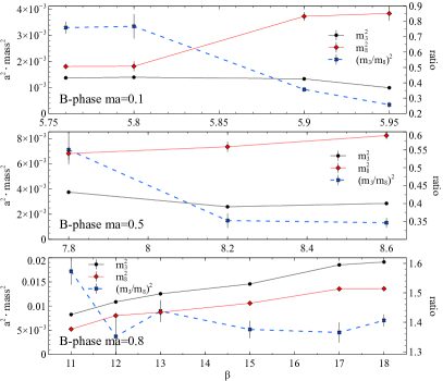
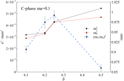
Figure 16: Results for the masses $m_{3}^{2}$ and $m_{8}^{2}$ in lattice units (left B-phase, right C-phase). The ratio is also plotted as blue line and the axis on the right indicates the scale

From the normalized plots we can estimate the values of the masses $m_{3}^{2}$ and $m_{8}^{2}$ of Sec. IV.3 in each phase by fitting the peaks of the density plots to a Gaussian curve after converting the variables $(\theta_{1},\theta_{2})$ to $(\phi_{3},\phi_{8})$ along eq. (46). In the continuum theory the distribution density is controlled by $e^{-\int d^{3}x\,V_{\rm eff}(\phi)}$ where $V_{\rm eff}(\phi)\simeq\hbox{$\frac{1}{2}$}\{m_{3}^{2}(\phi_{3}-\phi_{3}^{\rm min})^{2}+m_{8}^{2}(\phi_{8}-\phi_{8}^{\rm min})^{2}\}$ around each minimum of $V_{\rm eff}(\phi)$. With the $SU(3)$ invariance taken into account, the distribution density $\rho(\theta_{1},\theta_{2})$ is given by

$$\hskip-28.45274pt\int d\theta_{1}d\theta_{2}\,\rho(\theta_{1},\theta_{2})=\int[dU]\,e^{-(vol)V_{\rm eff}(\theta_{1},\theta_{2})}$$ (65)

$$\hskip-28.45274pt=\int d\theta_{1}d\theta_{2}\,\prod_{j<k}\sin^{2}\hbox{$\frac{1}{2}$}(\theta_{j}-\theta_{k})e^{-(vol)V_{\rm eff}(\theta_{1},\theta_{2})}~{}.$$ (66)

In other words, $\rho(\theta_{1},\theta_{2})$ divided by the Haar measure (64) can be fitted with a Gaussian distribution around the minima of $V_{\rm eff}(\theta_{1},\theta_{2})$ (this assumes that the deviation from the Gaussian are negligible around the maxima, and we estimated this by the quality of the fits, always with $\chi^{2}\sim 1$ and even smaller for many fitting points). In this way we can obtain a qualitative comparison with the one-loop results in eqs. (57), (60) and (61). The left panels of Fig. 16 show the result for B-phase. We observe the mass ratio $m_{3}^{2}/m_{8}^{2}$ deviates from $1$ and its non-trivial dependence on the bare parameters: $m_{3}^{2}/m_{8}^{2}>1$ if $ma>0.5$ and $m_{3}^{2}/m_{8}^{2}<1$ for lighter masses. On the other hand, in the C-phase, as seen in the right panel of the figure, we obtain the degenerate mass $m_{3}^{2}(\simeq m_{8}^{2})$ which is increasing for $mR\rightarrow 0$ ($\beta\rightarrow\infty$) as expected. For the A-phase, although the non-perfect cancellation obscures a clear peak, we can fairly conclude that $m_{3}\simeq m_{8}$ from the tails of the distributions. From the one-loop calculation, one expect that the mass ratio should cross in the B-phase passing from the A/B transition to the B/C transition. We could not find a direct evidence of this crossing with our current data but we observe an inversion of the ordering in the highest mass region. In summary, we find a match of the mass (non)degeneracy pattern to the perturbative prediction in this analysis.

V.3 Phase structure with fundamental fermions

As a further test of the perturbative prediction in Sec. IV, we study the dependence of $P_{3}$ and $P_{8}$ on the boundary phase $\alpha_{\rm fd}$ for several values of $\beta$ in the presence of fundamental fermions. As explained in Sec. II.2, we introduce $\alpha_{\rm fd}$ through the boundary condition (15). This setup is formally equivalent to finite temperature QCD with an imaginary chemical potential $\nu=\pi+\alpha_{\rm fd}$. Roberge and Weiss Roberge and Weiss (1986) have already shown that the corresponding partition function with SU($N$) gauge symmetry is periodic in $\nu$ as

$$Z(\nu)=Z(\nu+2\pi/N)$$ (67)

and there are discontinuities (first order lines) at $\nu=2n\pi/N$ with $n=0,\cdots,N-1$. These discontinuities exist in a region of high $\beta$ down to some endpoints which require a non-perturbative study to be located. Several numerical simulations on the lattice, for example de Forcrand and Philipsen (2002); D’Elia and Lombardo (2003), have determined these points as well as the phase structure in the $(\beta,\alpha_{\rm fd})$ plane, i.e. the transition lines which were associated with chiral phase transitions and the breaking of the approximate $Z_{3}$ symmetry for $\alpha_{\rm fd}$.

We carry out a numerical simulation with $(N_{\rm ad},N_{\rm fd})=(0,4)$. The basic setup is the same as in ref. D’Elia and Lombardo (2003) except for the bare fermion mass being fixed to $ma=0.10$ in our case. Since we are interested in the symmetries of the Polyakov loop, we determine the locations of the transition points by the peak points of $\chi_{|P_{3}|}$. Other technical matters related to this simulation are briefly summarized in Appendix C.

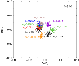
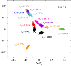
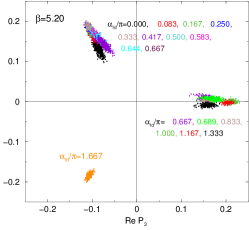
Figure 17: Distributions of $P_{3}$ obtained on gauge ensembles with a variation of $\alpha_{\rm fd}$ for $\beta=5.00$ (left), $5.15$ (center) and $5.20$ (right). The degrees of $\alpha_{\rm fd}$ used in the calculation are indicated with the corresponding data. Overall, data points with same degrees of $\alpha_{\rm fd}$ are indicated by same colors.

We compute the Polyakov loop in a region of the $(\beta,\alpha_{\rm fd})$ plane which covers the known phase structure. The resulting distributions of $P_{3}$ are shown in Fig. 17 for $\beta=5.00$ (left), $5.15$ (center) and $5.20$ (right). In each panel, we cover the range of $\alpha_{\rm fd}$ from $0$ to $5\pi/3$. For $\beta=5.00$, the sizable shift of the data from the origin is caused by the non-zero value of $(ma)^{-1}$, which breaks the ${\rm Z}_{3}$ symmetry. We observe a continuous change of ${P_{3}}$ as a function of $\alpha_{\rm fd}$ in this case. This behavior does not change even at $\beta=5.15$. On the other hand, the discontinuity of $P_{3}$ around $\alpha_{\rm fd}=2\pi/3$ is clearly visible for $\beta=5.20$. In particular, we find that the data at $\alpha_{\rm fd}=2\pi/3$ is in the $A_{1}$ phase or the $A_{2}$ depending on the initial configuration in HMC. This is the indication of the non-analyticity of $\theta$. For a better illustration of this behavior, in Fig. 18, we plot the phase ${\rm arg}(P_{3})$ as a function of $\alpha_{\rm fd}$. As seen in the figure, the transition from a continuous behavior to a discontinuous one around $\alpha_{\rm fd}=2\pi/3$ becomes more evident for increasing $\beta$. From the location of the peaks of $\chi_{P_{3}}$ we can draw the phase diagram of Fig. 18. We note that our data do not differ significantly from the results of e.g. ref. D’Elia and Lombardo (2003) with $ma=0.05$. It suggests that no significant mass dependence of the phase structure is expected. Because the perturbative region is realized at large $\beta$, there would be a split of phases into three classes $A_{1}$,$A_{2}$ and $A_{3}$ as described in eq. (45) and Figs. 4 and 5.

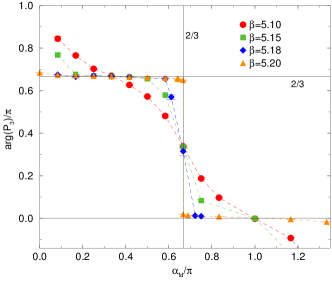
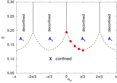
Figure 18: (Left) ${\rm arg}(P_{3})$ as a function of $\alpha_{\rm fd}$ with various values of $\beta$. (Right) Phase diagram of the $N_{\rm fd}=4$ fundamental fermion case. Solid lines indicate discontinuity separating the $A$ phase in the period of $2\pi/3$. Dashed lines are the critical line drawn by connecting the actual data points (red squares) and its copy based on the symmetry and periodicity explained in the text.

VI Discussion

In this paper we explored the Hosotani mechanism of symmetry breaking in the SU(3) gauge theory on the $16^{3}\times 4$ lattice. The Polyakov loop, its eigenvalue phases, and the susceptibility were measured and analyzed in models with periodic adjoint fermions and with fundamental fermions with general boundary conditions. Among the four phases appearing in the SU(3) model with adjoint fermions Cossu and D’Elia (2009), the $A$, $B$, and $C$ phases are interpreted as the SU(3), SU(2)$\times$U(1), and U(1)$\times$U(1) phases classified from the location of the global minimum of the effective potential of the AB phases. We confirmed natural correspondence between the effective potential evaluated in perturbation theory on $R^{3}\times S^{1}$ and the distribution of phases of eigenvalues of the Polyakov loop in the lattice simulations. The correspondence was seen in the model with fundamental fermions with varying boundary conditions as well.

The next issue to be settled is the particle spectrum. If the SU(3) symmetry is broken, asymmetry in the particle spectrum must show up in two-point correlation functions of appropriate operators. This can be explored in 4D lattice simulations. It is important from the viewpoint of phenomenological applications. We would like to explain why and how the $W$ and $Z$ bosons become massive in the scheme of the Hosotani mechanism non-perturbatively.

In the end, we would need a five-dimensional simulation to have realistic gauge-Higgs unification models of electroweak interactions. The continuum limit of the 5D lattice gauge theory has been under debate in the literature. Furthermore, we will need chiral fermions in four dimensions. It is customary to start from gauge theory on orbifolds in phenomenology, however. Lattice gauge theory on orbifolds needs further refinement. We would like to come back to these issues in future.

Appendix A Useful formulas for $V_{\rm eff}(\theta)$

We need to evaluate the following building block

$$V(\theta,m) \equiv \frac{1}{2}\sum_{n=-\infty}^{\infty}\int\frac{d^{d-1}p}{(2\pi)^{d-1}}\ln\left[p^{2}+\frac{1}{R^{2}}\left(n+\frac{\theta}{2\pi}\right)^{2}+m^{2}\right],$$ (68)

in terms of which $V_{\rm eff}$ is written as in Eq. (37). We use the technique of the zeta regularization to write $V(\theta,m)=-\zeta^{\prime}(0)/2$, where $\zeta(s)$ is the generalized zeta function defined by

$$\zeta(s) = \frac{1}{\Gamma(s)}\sum_{n=-\infty}^{\infty}\int_{0}^{\infty}dt\,t^{s-1}$$ (69)

$$\times\int\frac{d^{d-1}p}{(2\pi)^{d-1}}\exp\left\{-t\left[p^{2}+\frac{1}{R^{2}}\left(n+\frac{\theta}{2\pi}\right)^{2}+m^{2}\right]\right\}.$$

Here $\Gamma(s)$ is the Gamma function. Performing integration with $p$ and using Poisson’s summation formula,

$$\sum_{n=-\infty}^{\infty}\exp\left[-t\left(\frac{2\pi n+\theta}{2\pi R}\right)^{2}\right] = \frac{2\pi R}{\sqrt{4\pi t}}\sum_{\ell=-\infty}^{\infty}\exp\left(-\frac{(2\pi R)^{2}\ell^{2}}{4t}+i\ell\theta\right),$$ (70)

we obtain

$$\zeta(s) = \frac{\pi^{\frac{d-1}{2}}}{(2\pi)^{d-1}\Gamma(s)}\frac{2\pi R}{\sqrt{4\pi}}\sum_{n=-\infty}^{\infty}e^{in\theta}\int_{0}^{\infty}dt\,t^{s-\frac{d}{2}-1}\exp\left[-\frac{(2\pi R)^{2}n^{2}}{4t}-tm^{2}\right],$$ (71)

The $n=0$ part, though divergent, can be dropped as it is $\theta$-independent.

Using a formula

$$\int_{0}^{\infty}dt\,t^{-\nu-1}\exp\left[-tm^{2}-\frac{(2\pi R)^{2}n^{2}}{4t}\right] = \frac{2^{1+\nu}}{(2\pi R)^{2\nu}n^{2\nu}}(2\pi Rnm)^{\nu}K_{\nu}(2\pi Rnm),$$ (72)

and taking $s\to 0$ limit for $\zeta^{\prime}(s)$, we obtain

$$V(\theta,m) = -\frac{1}{2^{\frac{d}{2}-1}\pi^{d/2}(2\pi R)^{d-1}}\sum_{n=1}^{\infty}\frac{\cos n\theta-1}{n^{d}}\tilde{B}_{d/2}(2\pi Rnm).$$ (73)

where $\tilde{B}_{\delta}(x)\equiv x^{\delta}K_{\delta}(x)$. Normalizing by a factor $\tilde{B}_{d/2}(0)\equiv\lim_{x\to 0}\tilde{B}_{d/2}(x)=2^{\frac{d}{2}-1}\Gamma(d/2)$, we finally obtain

$$V(\theta,m) = -\frac{\Gamma(d/2)}{\pi^{d/2}(2\pi R)^{d-1}}\sum_{n=1}^{\infty}\frac{\cos n\theta-1}{n^{d}}B_{d/2}(2\pi Rnm)$$ (74)

which has been used in (40).

It would be useful to give another expression of $V(\theta,m)$, which has been obtained in Refs. Hatanaka and Hosotani (2012); Falkowski (2007);

$$V(\theta,m)=\frac{\displaystyle 1}{\displaystyle\Gamma(\tfrac{d-1}{2})(4\pi)^{\frac{d-1}{2}}R^{d-1}}\int_{mR}^{\infty}dt\,t\left(t^{2}-(mR)^{2}\right)^{\frac{d-3}{2}}\ln\left[1+\frac{\sin^{2}(\theta/2)}{\sinh^{2}(\pi t)}\right].$$ (75)

In both expressions (74) and (75), the $\theta$-independent constants have been chosen such that $V(0,m)=0$.

Appendix B Match to the weak coupling regime

We also check the agreement of the eigenvalue distribution of the Wilson line with the perturbative prediction in weak coupling regime, $\beta\rightarrow+\infty$ (that implies a compactification radius shrinking to zero as well as the 3d volume – with a ratio of 4 in our case), for $N_{\rm fd}=4$ fundamental fermions and $N_{\rm ad}=2$ adjoint fermions with periodic boundary conditions. Based on the analysis of Sec. III, the perturbative predictions for $\Delta\theta_{j}$’s are

• Fundamental fermions with periodic boundary condition
  In this case, the gauge symmetry is never broken. The true vacua of the effective potential are realized at $({\theta}_{1},{\theta_{2}},{\theta_{3}})=(-\frac{2\pi}{3},-\frac{2\pi}{3},-\frac{2\pi}{3})$ or $(\frac{2\pi}{3},\frac{2\pi}{3},\frac{2\pi}{3})$, see Fig. 4. In both vacua, the angle of the Wilson line phase ($\Delta\theta_{i}$) is

  $$(\Delta\theta_{1},\Delta\theta_{2},\Delta\theta_{3}) = (0,0,0).$$ (76)

• Adjoint fermions with periodic boundary condition
  In this case, the SU($3$) gauge symmetry is broken to U($1$) $\times$ U($1$). The true vacua are realized at $({\theta}_{1},{\theta_{2}},{\theta_{3}})=(0,\frac{2\pi}{3},-\frac{2\pi}{3})$ and the permutations, thus all eigenvalues of the Wilson line are not degenerate. We expect that

  $$(\Delta\theta_{1},\Delta\theta_{2},\Delta\theta_{3}) = (\tfrac{2\pi}{3},\tfrac{2\pi}{3},\tfrac{4\pi}{3}),\ \ (0\leq\Delta\theta_{j}<2\pi)$$ (77)

  with all possible permutations. In any case the peaks of the distribution are expected at $\pm\frac{2\pi}{3}$.

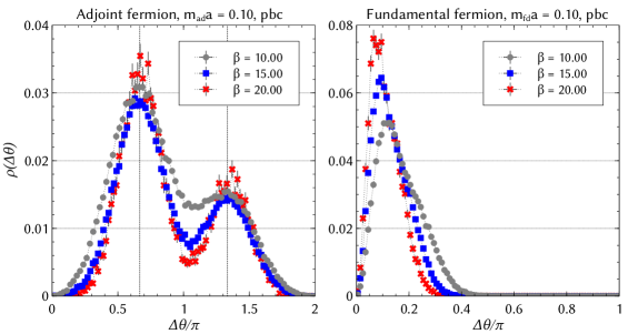
Figure 19: Density plots of $\Delta\theta_{i}$ ($i=1,2,3$) for $ma=0.10$ with the periodic boundary condition for adjoint and fundamental fermions, respectively. In the vertical axis the total density fraction is reported. For the readability, in the adjoint fermions case, we draw two lines to identify the expected peak locations $\Delta\theta_{i}=2\pi/3$ and $4\pi/3$.

Figure 19 shows the histograms of $\Delta\theta_{1},\Delta\theta_{2}$ and $\Delta\theta_{3}$ densities. The left and right panels show the results in the case of adjoint and fundamental fermions, respectively. In both cases, the fermion bare mass is fixed at $ma=0.10$ and the boundary condition is periodic. We change the value of $\beta=10.0,15.0$ and $20.0$.

In the case of the presence of adjoint fermions, the distribution drift towards the double peaks expected around $2\pi/3$ and $4\pi/3$ with the ratio 2 to 1 as indicated in (77).

In the case of fundamental fermions we find the position of the peaks approaches $\Delta\theta_{i}=0$, including the effect of the Haar measure that suppresses exactly the $\Delta\theta_{i}\simeq 0$ configurations. The exponential shrinking of the 3d volume does not seem to affect the matching of our results with the 1-loop prediction.

Appendix C Lattice technical details

In this section we describe some details of our lattice simulations.

The algorithm to generate the configurations is the Hybrid Monte Carlo (HMC) Duane et al. (1987); Gottlieb et al. (1987) for both adjoint and fundamental fermions. We obtain a new configuration by $N_{MD}$ steps of evolution of the molecular dynamics trajectory of size $\tau=1$.

In the case of adjoint fermions, the molecular dynamics integrator is the Omelyan Omelyan et al. (2002) with Hasenbush preconditioning Hasenbusch (2001). Using $N_{\rm MD}=25$ and $\Delta\tau=0.04$, we obtain an acceptance rate greater than 90%. We accumulate 4,000 - 14,000 trajectories depending on the parameter set $(ma,\beta)$. For the fundamental fermions case, by setting $N_{\rm MD}=50$ and $\Delta\tau=0.02$ in the standard leapfrog integrator, we obtain acceptance rate $\stackrel{{\scriptstyle>}}{{{}_{\sim}}}80\%$. Depending on the value of $(\beta,\alpha_{\rm fd})$, we accumulate 2,500 - 110,000 trajectories depending on the significance of signal.

The observables $P_{3}$ and $P_{8}$ are computed every 10 generated configurations. For the error analysis, we employ the unbiased jackknife method in both cases. As a reference we report the values of some plaquette values for few values of $\beta$ and $ma$ in Table 3.

Table 3: Plaquette and $|P_{3}|$ for some selected $\beta$ and $ma$ values for reference. Left: adjoint fermion case, Right: fundamental fermion case with $\alpha_{\rm fd}=0$.

$\beta$	$ma$	plaquette	$|P_{3}|\times 10^{2}$
5.30	0.1	0.5087(5)	0.88(4)
5.46	0.1	0.5671(1)	13.4(2)
5.75	0.1	0.6081(1)	7.9(3)
5.95	0.1	0.6279(1)	7.1(4)
6.00	0.1	0.6325(1)	6.1(6)
6.50	0.1	0.6696(8)	2.6(3)
5.50	0.5	0.5272(4)	1.20(8)
6.00	0.5	0.6089(2)	25.4(4)
7.00	0.5	0.6817(4)	35(1)
8.00	0.5	0.7285(7)	11(1)
9.00	0.5	0.7617(10)	6(2)

$\beta$	$ma$	plaquette	$|P_{3}|\times 10^{2}$
4.900	0.1	0.4224(1)	1.73(2)
5.000	0.1	0.4433(2)	1.97(3)
5.100	0.1	0.4702(4)	2.83(3)
5.150	0.1	0.4872(2)	3.71(4)
5.180	0.1	0.4997(2)	4.88(5)
5.190	0.1	0.5043(3)	5.53(11)
5.195	0.1	0.5167(5)	13.52(34)
5.200	0.1	0.5203(4)	15.85(10)
5.205	0.1	0.5222(4)	15.87(35)
5.210	0.1	0.5238(5)	16.32(51)
5.220	0.1	0.5269(5)	17.28(53)

References

- Hosotani (1983) Y. Hosotani, Phys.Lett. B126, 309 (1983).
- Davies and McLachlan (1988) A. Davies and A. McLachlan, Phys.Lett. B200, 305 (1988).
- Davies and McLachlan (1989) A. Davies and A. McLachlan, Nucl.Phys. B317, 237 (1989).
- Hosotani (1989) Y. Hosotani, Annals Phys. 190, 233 (1989).
- Hatanaka et al. (1998) H. Hatanaka, T. Inami, and C. Lim, Mod.Phys.Lett. A13, 2601 (1998), arXiv:hep-th/9805067 [hep-th] .
- Burdman and Nomura (2003) G. Burdman and Y. Nomura, Nucl.Phys. B656, 3 (2003), arXiv:hep-ph/0210257 [hep-ph] .
- Csaki et al. (2003) C. Csaki, C. Grojean, and H. Murayama, Phys.Rev. D67, 085012 (2003), arXiv:hep-ph/0210133 [hep-ph] .
- Agashe et al. (2005) K. Agashe, R. Contino, and A. Pomarol, Nucl.Phys. B719, 165 (2005), arXiv:hep-ph/0412089 [hep-ph] .
- Cacciapaglia et al. (2006) G. Cacciapaglia, C. Csaki, and S. C. Park, JHEP 0603, 099 (2006), arXiv:hep-ph/0510366 [hep-ph] .
- Medina et al. (2007) A. D. Medina, N. R. Shah, and C. E. Wagner, Phys.Rev. D76, 095010 (2007), arXiv:0706.1281 [hep-ph] .
- Hosotani and Sakamura (2007) Y. Hosotani and Y. Sakamura, Prog.Theor.Phys. 118, 935 (2007), arXiv:hep-ph/0703212 [hep-ph] .
- Adachi et al. (2007) Y. Adachi, C. Lim, and N. Maru, Phys.Rev. D76, 075009 (2007), arXiv:0707.1735 [hep-ph] .
- Adachi et al. (2009a) Y. Adachi, C. Lim, and N. Maru, Phys.Rev. D79, 075018 (2009a), arXiv:0901.2229 [hep-ph] .
- Adachi et al. (2009b) Y. Adachi, C. Lim, and N. Maru, Phys.Rev. D80, 055025 (2009b), arXiv:0905.1022 [hep-ph] .
- Hosotani et al. (2008) Y. Hosotani, K. Oda, T. Ohnuma, and Y. Sakamura, Phys.Rev. D78, 096002 (2008), arXiv:0806.0480 [hep-ph] .
- Hosotani et al. (2009) Y. Hosotani, P. Ko, and M. Tanaka, Phys.Lett. B680, 179 (2009), arXiv:0908.0212 [hep-ph] .
- Haba et al. (2010) N. Haba, Y. Sakamura, and T. Yamashita, JHEP 1003, 069 (2010), arXiv:0908.1042 [hep-ph] .
- Hosotani et al. (2010) Y. Hosotani, S. Noda, and N. Uekusa, Prog.Theor.Phys. 123, 757 (2010), arXiv:0912.1173 [hep-ph] .
- Hosotani et al. (2011) Y. Hosotani, M. Tanaka, and N. Uekusa, Phys.Rev. D84, 075014 (2011), arXiv:1103.6076 [hep-ph] .
- Adachi et al. (2012) Y. Adachi, N. Kurahashi, C. Lim, and N. Maru, JHEP 1201, 047 (2012), arXiv:1103.5980 [hep-ph] .
- Funatsu et al. (2013) S. Funatsu, H. Hatanaka, Y. Hosotani, Y. Orikasa, and T. Shimotani, Phys.Lett. B722, 94 (2013), arXiv:1301.1744 [hep-ph] .
- Maru and Okada (2013a) N. Maru and N. Okada, Phys.Rev. D87, 095019 (2013a), arXiv:1303.5810 [hep-ph] .
- Maru and Okada (2013b) N. Maru and N. Okada, Phys.Rev. D88, 037701 (2013b), arXiv:1307.0291 [hep-ph] .
- Cossu and D’Elia (2009) G. Cossu and M. D’Elia, JHEP 0907, 048 (2009), arXiv:0904.1353 [hep-lat] .
- Unsal and Yaffe (2008) M. Unsal and L. G. Yaffe, Phys.Rev. D78, 065035 (2008), arXiv:0803.0344 [hep-th] .
- Hosotani (2012) Y. Hosotani, AIP Conf.Proc. 1467, 208 (2012), arXiv:1206.0552 [hep-ph] .
- Kashiwa and Misumi (2013) K. Kashiwa and T. Misumi, JHEP 1305, 042 (2013), arXiv:1302.2196 [hep-ph] .
- Irges and Knechtli (2007) N. Irges and F. Knechtli, Nucl.Phys. B775, 283 (2007), arXiv:hep-lat/0609045 [hep-lat] .
- Irges and Knechtli (2009) N. Irges and F. Knechtli, Nucl.Phys. B822, 1 (2009), arXiv:0905.2757 [hep-lat] .
- de Forcrand et al. (2010) P. de Forcrand, A. Kurkela, and M. Panero, JHEP 1006, 050 (2010), arXiv:1003.4643 [hep-lat] .
- Del Debbio et al. (2012) L. Del Debbio, A. Hart, and E. Rinaldi, JHEP 1207, 178 (2012), arXiv:1203.2116 [hep-lat] .
- Irges et al. (2012) N. Irges, F. Knechtli, and K. Yoneyama, Nucl.Phys. B865, 541 (2012), arXiv:1206.4907 [hep-lat] .
- Irges et al. (2013) N. Irges, F. Knechtli, and K. Yoneyama, Phys.Lett. B722, 378 (2013), arXiv:1212.5514 .
- Knechtli et al. (2012) F. Knechtli, M. Luz, and A. Rago, Nucl.Phys. B856, 74 (2012), arXiv:1110.4210 [hep-lat] .
- Hatanaka (1999) H. Hatanaka, Prog.Theor.Phys. 102, 407 (1999), arXiv:hep-th/9905100 [hep-th] .
- Hosotani (2005) Y. Hosotani, Proceedings of SCGT2004 , 17 (2005), arXiv:hep-ph/0504272 [hep-ph] .
- Gattringer and Lang (2010) C. Gattringer and C. B. Lang, Lect.Notes Phys. 788, 1 (2010).
- Duane et al. (1987) S. Duane, A. Kennedy, B. Pendleton, and D. Roweth, Phys.Lett. B195, 216 (1987).
- Gottlieb et al. (1987) S. A. Gottlieb, W. Liu, D. Toussaint, R. Renken, and R. Sugar, Phys.Rev. D35, 2531 (1987).
- Anber and Unsal (2013) M. M. Anber and M. Unsal, (2013), arXiv:1309.4394 [hep-th] .
- Ogilvie (2012) M. C. Ogilvie, J.Phys. A45, 483001 (2012), arXiv:1211.2843 [hep-th] .
- Roberge and Weiss (1986) A. Roberge and N. Weiss, Nucl.Phys. B275, 734 (1986).
- Karsch and Lutgemeier (1999) F. Karsch and M. Lutgemeier, Nucl.Phys. B550, 449 (1999), arXiv:hep-lat/9812023 [hep-lat] .
- Fukugita et al. (1989) M. Fukugita, M. Okawa, and A. Ukawa, Phys.Rev.Lett. 63, 1768 (1989).
- Bialas et al. (2005) P. Bialas, A. Morel, and B. Petersson, Nucl.Phys. B704, 208 (2005), arXiv:hep-lat/0403027 [hep-lat] .
- Myers and Ogilvie (2008) J. C. Myers and M. C. Ogilvie, Phys.Rev. D77, 125030 (2008), arXiv:0707.1869 [hep-lat] .
- Simon (1995) B. Simon, Representations of Finite and Compact Groups (American Mathematical Society, 1995).
- Morningstar and Peardon (2004) C. Morningstar and M. J. Peardon, Phys.Rev. D69, 054501 (2004), arXiv:hep-lat/0311018 [hep-lat] .
- Note (1) The most problematic points are the minima of the Haar measure where the numerically calculated histogram has almost zero occupation number and a perfect cancelation is required to get the signal. At these points we can get divergent results. In the B and C phases these are essentially harmless since we know by theoretical arguments that there should be nothing there. It is more dangerous in the A phase where the peak of the distribution is poorly determined.
- Poppitz et al. (2013) E. Poppitz, T. Schäfer, and M. Ünsal, JHEP 1303, 087 (2013), arXiv:1212.1238 .
- de Forcrand and Philipsen (2002) P. de Forcrand and O. Philipsen, Nucl.Phys. B642, 290 (2002), arXiv:hep-lat/0205016 [hep-lat] .
- D’Elia and Lombardo (2003) M. D’Elia and M.-P. Lombardo, Phys.Rev. D67, 014505 (2003), arXiv:hep-lat/0209146 [hep-lat] .
- Hatanaka and Hosotani (2012) H. Hatanaka and Y. Hosotani, Phys.Lett. B713, 481 (2012), arXiv:1111.3756 [hep-ph] .
- Falkowski (2007) A. Falkowski, Phys.Rev. D75, 025017 (2007), arXiv:hep-ph/0610336 [hep-ph] .
- Omelyan et al. (2002) I. P. Omelyan, I. M. Mryglod, and R. Folk, Phys. Rev. E 65, 056706 (2002).
- Hasenbusch (2001) M. Hasenbusch, Phys.Lett. B519, 177 (2001), arXiv:hep-lat/0107019 [hep-lat] .