17th September, 2013

Summary

Fast variational approximate algorithms are developed for Bayesian semiparametric regression when the response variable is a count, i.e. a non-negative integer. We treat both the Poisson and Negative Binomial families as models for the response variable. Our approach utilizes recently developed methodology known as non-conjugate variational message passing. For concreteness, we focus on generalized additive mixed models, although our variational approximation approach extends to a wide class of semiparametric regression models such as those containing interactions and elaborate random effect structure. Keywords: Approximate Bayesian inference; Generalized additive mixed models; Mean field variational Bayes; Penalized splines; Real-time semiparametric regression.

1 Introduction

A pervasive theme impacting Statistics in the mid-2010s is the increasing prevalence of data that are big in terms of volume and/or velocity. One of many relevant articles is Michalak et al. (2012), where the need for systems that perform real-time streaming data analyses is described. The analysis of high volume data and velocity data requires approaches that put a premium on speed, possibly at the cost of accuracy. Within this context, we develop methodology for fast, and possibly online, semiparametric regression analyses in the case of count response data.

Semiparametric regression, as defined in Ruppert, Wand & Carroll (2009), is a fusion between parametric and nonparametic regression that integrates low-rank penalized splines and wavelets, mixed models and Bayesian inference methodology. In Luts, Broderick & Wand (2013) we developed semiparametric regression algorithms for high volume and velocity data using a mean field variational Bayes (MFVB) approach. It was argued there that MFVB, or similar methodology, is necessary for fast batch and online semiparametric regression analyses, and that more traditional methods such as Markov chain Monte Carlo (MCMC) are not feasible. However, the methodology of Luts, Broderick & Wand (2013) was restricted to fitting Gaussian and Bernoulli response models. Extension to various other response distributions, such as $t$, Skew Normal and Generalized Extreme Value is relatively straightforward using approaches described in Wand et al. (2011). However count response distributions such as the Poisson and Negative Binomial distribution have received little attention in the MFVB literature. Recently Tan & Nott (2013) used an extension of MFVB, known as non-conjugate variational message passing, to handle Poisson mixed models for longitudinal data and their lead is followed here for more general classes of count response semiparametric regression models.

In generalized response regression, the Poisson distribution is often bracketed with the Bernoulli distribution since both are members of the one-parameter exponential family. However, variational approximations for Poisson response models are not as forthcoming as those with Bernoulli responses. Jaakkola & Jordan (2000) derived a lower bound on the Bayesian logistic regression marginal likelihood that leads to tractable approximate variational inference. As explained in Girolami & Rogers (2006) and Consonni & Marin (2007), the Albert & Chib (1993) auxiliary variable representation of Bayesian probit regression leads to a different type of variational approximation method for binary response regression. There do not appear to be analogues of these approaches for Bayesian Poisson regression and different routes are needed. An effective solution is afforded by a recent extension of MFVB, due to Knowles & Minka (2011), known as non-conjugate variational message passing. The Negative Binomial distribution can also be handled using non-conjugate variational message passing, via its well-known representation as a Poisson-Gamma mixture (e.g. Lawless, 1987). We adopt such an approach here and develop MFVB algorithms for both Poisson and Negative Binomial semiparametric regression models. For ease of presentation, we restrict attention to the special case of generalized additive mixed models, but extension to other semiparametric regression models is straightforward.

Section 2 lays down required notation and distributional results. It also provides a brief synopsis of non-conjugate mean field variational Bayes. The models are then described in Section 3. The article’s centerpiece is Section 4, which is where the variational inference algorithms for count response semiparametric regression are presented. In Section 5 we describe real-time fitting of such models. Numerical illustrations are given in Section 6 and an appendix contains derivations of the aforementioned variational algorithms.

2 Background Material

The specification of the models and their fitting via variational algorithms requires several definitions and results, and are provided in this section.

2.1 Distributional Definitions

Table 1 lists all distributions used in this article. In particular, the parametrization of the corresponding density functions and probability functions is provided.

distribution	density/probability function in $x$	abbreviation
Poisson	$\lambda^{x}\,e^{-\lambda}/x!;\quad x=0,1,\ldots$	$\mbox{Poisson}(\lambda)$
Negative Binomial	$\displaystyle{\frac{\kappa^{\kappa}\Gamma(x+\kappa)\mu^{x}}{\Gamma(\kappa)(\kappa+\mu)\Gamma(x+1)}};\ x=0,1\ldots;$	$\mbox{Negative-Binomial}(\mu,\kappa)$
	$\kappa,\mu>0$
Uniform	$1/(b-a);\quad a<x<b$	$\mbox{Uniform}(a,b)$
Multivariate Normal	$|2\pi\boldsymbol{\Sigma}|^{-1/2}\,\exp\{-{\textstyle{\frac{1}{2}}}(\boldsymbol{x}-\boldsymbol{\mu})^{T}\boldsymbol{\Sigma}^{-1}(\boldsymbol{x}-\boldsymbol{\mu})\}$	$N(\boldsymbol{\mu},\boldsymbol{\Sigma})$
Gamma	$\displaystyle{\frac{B^{A}\,x^{A-1}e^{-B\,x}}{\Gamma(A)}};\quad x>0;\ A,B>0$	$\mbox{Gamma}(A,B)$
Inverse-Gamma	$\displaystyle{\frac{B^{A}\,x^{-A-1}e^{-B/x}}{\Gamma(A)}};\quad x>0;\ A,B>0$	$\mbox{Inverse-Gamma}(A,B)$
Half-Cauchy	$\displaystyle{\frac{2\sigma}{\pi(x^{2}+\sigma^{2})}};\quad x>0;\ \sigma>0$	$\mbox{Half-Cauchy}(\sigma)$

Table 1: Distributions used in this article and their corresponding density/probability functions.

2.2 Distributional Results

The variational inference algorithms given in Section 4 make use of the following distributional results:

Result 1. Let $x$ and $a$ be random variables such that

$$x|\,a\sim\mbox{Poisson}(a)\quad\mbox{\em and}\quad a\sim\mbox{Gamma}(\kappa,\kappa/\mu).$$

Then $x\sim\mbox{Negative-Binomial}(\mu,\kappa)$.

Result 2. Let $x$ and $a$ be random variables such that

$$x|\,a\sim\mbox{Inverse-Gamma}(1/2,1/a)\quad\mbox{\em and}\quad a\sim\mbox{Inverse-Gamma}({\textstyle{\frac{1}{2}}},1/A^{2}).$$

Then $\sqrt{x}\sim\mbox{Half-Cauchy}(A)$.

Result 1 is a relatively well-known distribution theoretic result (e.g. Lawless, 1987). Result 2 is related to established results concerning the $F$ distribution family, and this particular version is taken from Wand et al. (2011).

2.3 Non-conjugate Variational Message Passing

Non-conjugate variational message passing (Knowles & Minka, 2011) is an extension of MFVB. It can yield tractable variational approximate inference in situations where ordinary MFVB is intractable.

MFVB relies on approximating the joint posterior density function $p(\boldsymbol{\theta}|\boldsymbol{y})$ by a product form $q(\boldsymbol{\theta})=\prod_{i=1}^{d}q(\boldsymbol{\theta}_{i})$, where $\boldsymbol{\theta}$ corresponds to the hidden nodes in Figure 1. The optimal $q$-density functions, denoted by $q^{*}(\boldsymbol{\theta}_{i})$, are those that minimize the Kullback-Leibler divergence

$$\int q(\boldsymbol{\theta})\log\left(\frac{q(\boldsymbol{\theta})}{p(\boldsymbol{\theta}|\boldsymbol{y})}\right)\,d\boldsymbol{\theta}.\\$$

An equivalent optimization problem represents maximizing the lower bound on the marginal likelihood $p(\boldsymbol{y})$:

$$\underline{p}(\boldsymbol{y};q)\equiv\exp\left\{\int q(\boldsymbol{\theta})\log\left(\frac{p(\boldsymbol{\theta},\boldsymbol{y})}{q(\boldsymbol{\theta})}\right)\,d\boldsymbol{\theta}\right\}.\\$$

The optimal $q$-density functions can be shown to satisfy

$$q^{*}(\boldsymbol{\theta}_{i})\propto\exp\left[E_{-\boldsymbol{\theta}_{i}}\left\{\log p(\boldsymbol{\theta}_{i}|\mbox{rest})\right\}\right],\quad 1\leq i\leq d,\\$$

where $E_{-\boldsymbol{\theta}_{i}}$ denotes expectation with respect to the density $\prod_{j\neq i}q_{j}(\boldsymbol{\theta}_{j})$ and ‘rest’ denotes all random variables in the model other than $\boldsymbol{\theta}_{i}$.

In the event that one of the $E_{-\boldsymbol{\theta}_{i}}\left\{\log p(\boldsymbol{\theta}_{i}|\mbox{rest})\right\}$ is not tractable, let’s say the one corresponding to $q(\boldsymbol{\theta}_{j})$ for some $j\in\{1,\ldots,d\}$, non-conjugate variational message passing offers a way out (Knowles & Minka, 2011). It first postulates that $q(\boldsymbol{\theta}_{j})$ is an exponential family density function with natural parameter vector $\boldsymbol{\eta}_{j}$ and natural statistic $\boldsymbol{T}(\boldsymbol{\theta}_{j})$. The optimal parameters are then obtained via updates of the form

$$\boldsymbol{\eta}_{j}\leftarrow\left\{\text{var}\left(\boldsymbol{T}(\boldsymbol{\theta}_{j})\right)\right\}^{-1}\left\{{\sf D}_{\boldsymbol{\eta_{j}}}E_{\boldsymbol{\theta}}\left[\log p(\boldsymbol{\theta},\boldsymbol{y})\right]\right\},\\$$ (1)

where ${\sf D}_{\boldsymbol{x}}f$ is the derivative vector of $f$ with respect to $\boldsymbol{x}$ and $\text{var}(\boldsymbol{v})$ denotes the covariance matrix of random vector $\boldsymbol{v}$ (Magnus & Neudecker, 1999). Wand (2013) derived fully simplified expressions for (1) in case $q(\boldsymbol{\theta}_{j})$ has a Multivariate Normal density with mean $\boldsymbol{\mu}_{q(\theta_{j})}$ and covariance matrix $\boldsymbol{\Sigma}_{q(\theta_{j})}$

$$\begin{array}[]{l}\boldsymbol{\Sigma}_{q(\theta_{j})}\leftarrow\left\{-2\,\mbox{vec}^{-1}\left(\left[{\sf D}_{\mbox{vec}(\boldsymbol{\Sigma})}E_{\boldsymbol{\theta}}\left\{\log p(\boldsymbol{\theta},\boldsymbol{y})\right\}\right]^{T}\right)\right\}^{-1},\\[12.91663pt] \boldsymbol{\mu}_{q(\theta_{j})}\leftarrow\boldsymbol{\mu}_{q(\theta_{j})}+\boldsymbol{\Sigma}_{q(\theta_{j})}\left[{\sf D}_{\boldsymbol{\mu}}E_{\boldsymbol{\theta}}\left\{\log p(\boldsymbol{\theta},\boldsymbol{y})\right\}\right]^{T}\\ \end{array}$$ (2)

with $\text{vec}(\boldsymbol{A})$ denoting a vector formed by stacking the columns of matrix $\boldsymbol{A}$ underneath each other in order from left to right and $\text{vec}^{-1}(\boldsymbol{a})$ a matrix formed from listing the entries of vector $\boldsymbol{a}$ in a column-wise fashion in order from left to right.

3 Model descriptions

Count responses are most commonly modelled according to the Poisson and Negative Binomial distributions. The latter may be viewed as an extension of the former through the introduction of an additional parameter.

Throughout this section we use $\stackrel{{\scriptstyle{\tiny\mbox{ind.}}}}{{\sim}}$ to denote “independently distributed as”.

3.1 Poisson additive mixed model

We work with the following class of Bayesian Poisson additive mixed models:

$$\begin{array}[]{c}y_{i}|\,\boldsymbol{\beta},\boldsymbol{u}\stackrel{{\scriptstyle{\tiny\mbox{ind.}}}}{{\sim}}\mbox{Poisson}[\exp\{(\boldsymbol{X}\boldsymbol{\beta}+\boldsymbol{Z}\boldsymbol{u})_{i}\}],\quad 1\leq i\leq n,\\[8.61108pt] \boldsymbol{u}|\,\sigma_{1}^{2},\ldots,\sigma_{r}^{2}\sim N(\boldsymbol{0},\mbox{blockdiag}(\sigma_{1}^{2}\,\boldsymbol{I}_{K_{1}},\ldots,\sigma_{r}^{2}\,\boldsymbol{I}_{K_{r}})),\\[8.61108pt] \boldsymbol{\beta}\sim N(\boldsymbol{0},\sigma_{\beta}^{2}\boldsymbol{I}_{p}),\quad\mbox{and}\quad\sigma_{\ell}\stackrel{{\scriptstyle{\tiny\mbox{ind.}}}}{{\sim}}\mbox{Half-Cauchy}(A_{\ell}),\quad 1\leq\ell\leq r.\end{array}$$ (3)

Here $\boldsymbol{y}$ is an $n\times 1$ vector of response variables, $\boldsymbol{\beta}$ is a $p\times 1$ vector of fixed effects, $\boldsymbol{u}$ is a vector of random effects, $\boldsymbol{X}$ and $\boldsymbol{Z}$ corresponding design matrices, and $\sigma_{1}^{2},\ldots,\sigma_{r}^{2}$ are variance parameters corresponding to sub-blocks of $\boldsymbol{u}$ of size $K_{1},\ldots,K_{r}$.

Result 2 of Section 2.2 allows us to replace $\sigma_{\ell}\stackrel{{\scriptstyle{\tiny\mbox{ind.}}}}{{\sim}}\mbox{Half-Cauchy}(A_{\ell})$ with

$$\quad\sigma_{\ell}^{2}\,|\,a_{\ell}\stackrel{{\scriptstyle{\tiny\mbox{ind.}}}}{{\sim}}\mbox{Inverse-Gamma}({\textstyle{\frac{1}{2}}},1/a_{\ell}),\quad a_{\ell}\stackrel{{\scriptstyle{\tiny\mbox{ind.}}}}{{\sim}}\mbox{Inverse-Gamma}({\textstyle{\frac{1}{2}}},1/A_{\ell}^{2}),\quad 1\leq\ell\leq r,$$

which is more amenable to variational inference.

Note that the $r=1$ version of (3) is treated in Wand (2013).

3.2 Negative Binomial additive mixed model

The Negative Binomial distribution is an extension of the Poisson distribution in that the former approaches a version of the latter as the shape parameter $\kappa\to\infty$ (see Table 1). The Negative Binomial shape parameter allows for a wider range of dependencies of the variance on the mean and can better handle over-dispersed count data.

The Bayesian Negative Binomial additive mixed model treated here is

$$\begin{array}[]{c}y_{i}|\,\boldsymbol{\beta},\boldsymbol{u}\stackrel{{\scriptstyle{\tiny\mbox{ind.}}}}{{\sim}}\mbox{Negative-Binomial}[\,\exp\{(\boldsymbol{X}\boldsymbol{\beta}+\boldsymbol{Z}\boldsymbol{u})_{i}\}],\quad 1\leq i\leq n,\\[8.61108pt] \boldsymbol{u}|\,\sigma_{1}^{2},\ldots,\sigma_{r}^{2}\sim N(\boldsymbol{0},\mbox{blockdiag}(\sigma_{1}^{2}\,\boldsymbol{I}_{K_{1}},\ldots,\sigma_{r}^{2}\,\boldsymbol{I}_{K_{r}})),\quad\boldsymbol{\beta}\sim N(\boldsymbol{0},\sigma_{\beta}^{2}\boldsymbol{I}_{p}),\\[12.91663pt] \quad\sigma_{\ell}\stackrel{{\scriptstyle{\tiny\mbox{ind.}}}}{{\sim}}\mbox{Half-Cauchy}(A_{\ell}),\quad 1\leq\ell\leq r,\ \mbox{and}\quad\kappa\sim\mbox{Uniform}\left(\kappa_{\text{min}},\kappa_{\text{max}}\right).\end{array}$$ (4)

Courtesy of Result 1 given in Section 2.2,

$$y_{i}|\,\boldsymbol{\beta},\boldsymbol{u},\kappa\stackrel{{\scriptstyle{\tiny\mbox{ind.}}}}{{\sim}}\mbox{Negative-Binomial}[\,\exp\{(\boldsymbol{X}\boldsymbol{\beta}+\boldsymbol{Z}\boldsymbol{u})_{i}\},\kappa],\quad 1\leq i\leq n,$$

can be replaced by

$$y_{i}|g_{i}\stackrel{{\scriptstyle{\tiny\mbox{ind.}}}}{{\sim}}\mbox{Poisson}\left(g_{i}\right),\quad g_{i}|\boldsymbol{\beta},\boldsymbol{u},\kappa\stackrel{{\scriptstyle{\tiny\mbox{ind.}}}}{{\sim}}\mbox{Gamma}\left(\kappa,\kappa\,\exp\{-(\boldsymbol{X}\boldsymbol{\beta}+\boldsymbol{Z}\boldsymbol{u})_{i}\}\right),\quad 1\leq i\leq n,$$

where $\boldsymbol{g}$ is the $n\times 1$ vector containing the $g_{i}$, $1\leq i\leq n$.

3.3 Directed Acyclic Graph Representations

Figure 1 provides a directed acyclic graph representation of models (3) and (4). Observed data are indicated by the shaded node while parameters, random effects and auxiliary variables are so-called hidden nodes. This visual representation shows that the Poisson case and Negative Binomial case have part of their graphs in common. The locality property of MFVB (e.g. Section 2 of Wand et al., 2011) means that the variational inference algorithms for the two models have some components in common. We take advantage of this in Section 4.

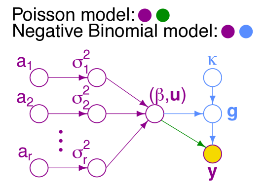
Figure 1: Directed acyclic graph corresponding to the models (3) and (4). The shaded node corresponds to the observed data. The color key at the top of the figure denotes the components of the graph corresponding to each model.

3.4 Extension to Unstructured Covariance Matrices for Random Effects

Section 2.3 of Luts, Broderick & Wand (2013) describes the extension to semiparametric models containing unstructured covariance matrices. Such extensions arise in the case of random intercept and slope models. A simple example of such a model having count responses is:

$$\begin{array}[]{c}y_{ij}|\beta_{0},\beta_{1},U_{i},V_{i}\stackrel{{\scriptstyle{\tiny\mbox{ind.}}}}{{\sim}}\mbox{Poisson}\{\exp(\beta_{0}+U_{i}+(\beta_{1}+V_{i})\,x_{ij})\},\quad 1\leq i\leq m,\quad 1\leq j\leq n_{i},\\[8.61108pt] \mbox{and}\quad\left[\begin{array}[]{c}U_{i}\\ V_{i}\\ \end{array}\right]\Big{|}\boldsymbol{\Sigma}\sim N(\boldsymbol{0},\boldsymbol{\Sigma}),\quad\mbox{where}\quad\boldsymbol{\Sigma}\equiv\left[\begin{array}[]{cc}\sigma_{u}^{2}&\rho_{uv}\,\sigma_{u}\,\sigma_{v}\\ \rho_{uv}\,\sigma_{u}\,\sigma_{v}&\sigma_{v}^{2}\end{array}\right].\end{array}$$

The advice given in Section 2.3 of Luts, Broderick & Wand (2013) concerning such extensions applies here as well.

3.5 Hyperparameter Default Values

With noninformativity in mind, reasonable default values for the hyperparameters in models (3) and (4) are

$$\sigma_{\beta}=A_{\ell}=10^{5},\quad\kappa_{\text{min}}=\textstyle{\frac{1}{100}}\quad\mbox{and}\quad\kappa_{\text{max}}=100,$$

assuming that the predictor data have been standardized to have zero mean and unit standard deviation.

All examples in this article use these hyperparameter settings with standardized predictor data, and then transform the results to the original units.

4 Variational Inference Scheme

We are now in a position to derive a variational inference scheme for fitting the Poisson and Negative Binomial additive mixed models described in Section 3 and displayed in Figure 1. In this section we work toward a variational inference algorithm that treats both models by taking advantage of their commonalities, but also recognizing the differences. The algorithm, which we call Algorithm 1, is given in Section 4.3.

4.1 Poisson Case

We first treat the Poisson additive mixed model (3). Ordinary MFVB begins with a product restriction such as

$$p(\boldsymbol{\beta},\boldsymbol{u},\sigma_{1}^{2},\ldots,\sigma_{r}^{2},a_{1},\ldots,a_{r}|\boldsymbol{y})\approx q(\boldsymbol{\beta},\boldsymbol{u})\,\,q(\sigma^{2}_{1},\ldots,\sigma^{2}_{r})\,q(a_{1},\ldots,a_{r}).$$ (5)

However, under (5), the optimal posterior density function of $(\boldsymbol{\beta},\boldsymbol{u})$ is

$$q^{*}(\boldsymbol{\beta},\boldsymbol{u})\propto\exp[E_{q(-(\boldsymbol{\beta},\boldsymbol{u}))}\{\log p(\boldsymbol{\beta},\boldsymbol{u}|\mbox{rest})\}]$$

and involves multivariate integrals that are not available in closed form. A non-conjugate variational message passing solution is one that instead works with

$$p(\boldsymbol{\beta},\boldsymbol{u},\sigma_{1}^{2},\ldots,\sigma_{r}^{2},a_{1},\ldots,a_{r}|\boldsymbol{y})\approx q(\boldsymbol{\beta},\boldsymbol{u};\boldsymbol{\mu}_{q(\boldsymbol{\beta},\boldsymbol{u})},\boldsymbol{\Sigma}_{q(\boldsymbol{\beta},\boldsymbol{u})})\,q(\sigma^{2}_{1},\ldots,\sigma^{2}_{r})\,q(a_{1},\ldots,a_{r})$$ (6)

where

$$q(\boldsymbol{\beta},\boldsymbol{u};\boldsymbol{\mu}_{q(\boldsymbol{\beta},\boldsymbol{u})},\boldsymbol{\Sigma}_{q(\boldsymbol{\beta},\boldsymbol{u})})\quad\mbox{is the}\quad N\left(\boldsymbol{\mu}_{q(\boldsymbol{\beta},\boldsymbol{u})},\boldsymbol{\Sigma}_{q(\boldsymbol{\beta},\boldsymbol{u})}\right)\quad\mbox{density function.}$$ (7)

In the appendix, we show that the optimal posterior densities for the variance and auxiliary parameters are:

$$\begin{array}[]{l}q^{*}(\sigma^{2}_{1},\ldots,\sigma^{2}_{r})\,\text{is the product of}\\[4.30554pt] \mbox{Inverse-Gamma}\left(\frac{K_{\ell}+1}{2},\mu_{q(1/a_{\ell})}+\frac{1}{2}\left\{\|\boldsymbol{\mu}_{q(\boldsymbol{u}_{\ell})}\|^{2}+\text{tr}\left(\boldsymbol{\Sigma}_{q(\boldsymbol{u}_{\ell})}\right)\right\}\right)\ \mbox{density functions,}\\[4.30554pt] \mbox{and}\ q^{*}(a_{1},\ldots,a_{r})\,\text{is the product of}\,\mbox{Inverse-Gamma}\left(1,\mu_{q(1/\sigma^{2}_{{\ell}})}+A^{-2}_{{\ell}}\right)\ \mbox{density}\\[4.30554pt] \text{functions, $1\leq\ell\leq r$,}\end{array}$$ (8)

where $\mu_{q(1/\sigma_{\ell}^{2})}\equiv\int_{0}^{\infty}(1/\sigma_{\ell}^{2})q(\sigma_{\ell}^{2})\,d\sigma_{\ell}^{2}$,  $\mu_{q(1/a_{\ell})}$ is defined analogously,

$$\boldsymbol{\mu}_{q(\boldsymbol{u}_{\ell})}\equiv\mbox{sub-vector of $\boldsymbol{\mu}_{q(\boldsymbol{\beta},\boldsymbol{u})}$ corresponding to $\boldsymbol{u}_{\ell}$}$$

and

$$\boldsymbol{\Sigma}_{q(\boldsymbol{u}_{\ell})}\equiv\mbox{sub-matrix of $\boldsymbol{\Sigma}_{q(\boldsymbol{\beta},\boldsymbol{u})}$ corresponding to $\boldsymbol{u}_{\ell}$.}$$

The interdependencies between the parameters in these optimal density functions, combined with the updates for $\boldsymbol{\mu}_{q(\boldsymbol{\beta},\boldsymbol{u})}$ and $\boldsymbol{\Sigma}_{q(\boldsymbol{\beta},\boldsymbol{u})}$ given by (LABEL:eq:updatesMatt) give rise to an iterative scheme for their solution, and is encompassed in Algorithm 1.

Algorithm 1 also uses the variational lower bound on the marginal log-likelihood. For model (3) and restriction (6) it has the explicit expression

$$\begin{array}[]{rcl}\log\underline{p}(\boldsymbol{y};q)&=&\frac{P}{2}-r\log(\pi)-\frac{p}{2}\log(\sigma^{2}_{\beta})+\frac{1}{2}\log|\boldsymbol{\Sigma}_{q(\boldsymbol{\beta},\boldsymbol{u})}|-\boldsymbol{1}^{T}\log(\boldsymbol{y}!)\\[8.61108pt] &&-\frac{1}{2\sigma^{2}_{\beta}}\{\|\boldsymbol{\mu}_{q(\boldsymbol{\beta})}\|^{2}+\text{tr}(\boldsymbol{\Sigma}_{q(\boldsymbol{\beta})})\}+\sum_{\ell=1}^{r}\Big{[}\mu_{q(1/a_{\ell})}\mu_{q(1/\sigma_{\ell}^{2})}\\[8.61108pt] &&-\log(A_{\ell})-\log\{\mu_{q(1/\sigma_{\ell}^{2})}+A_{\ell}^{-2}\}+\log\left\{\Gamma\left(\frac{K_{\ell}+1}{2}\right)\right\}\\[8.61108pt] &&-\frac{K_{\ell}+1}{2}\log(\mu_{q(1/a_{\ell})}+\frac{1}{2}\{\|\boldsymbol{\mu}_{q(\boldsymbol{u}_{\ell})}\|^{2}+\text{tr}(\boldsymbol{\Sigma}_{q(\boldsymbol{u}_{\ell})})\}\Big{]}\\[8.61108pt] &&+\boldsymbol{y}^{T}\boldsymbol{C}\boldsymbol{\mu}_{q(\boldsymbol{\beta},\boldsymbol{u})}-\boldsymbol{1}^{T}\exp\left\{\boldsymbol{C}\boldsymbol{\mu}_{q(\boldsymbol{\beta},\boldsymbol{u})}+\frac{1}{2}\mbox{diagonal}(\boldsymbol{C}\boldsymbol{\Sigma}_{q(\boldsymbol{\beta},\boldsymbol{u})}\boldsymbol{C}^{T})\right\}.\\ \end{array}$$

Here and elsewhere,

$$\mbox{diagonal}(\boldsymbol{M})\equiv\mbox{vector of diagonal entries of $\boldsymbol{M}$}$$

for any square matrix $\boldsymbol{M}$. Also,

$$\boldsymbol{C}\equiv[\boldsymbol{X}\ \boldsymbol{Z}]\quad\mbox{and}\quad P\equiv\mbox{number of columns in $\boldsymbol{C}$}=p+\sum_{\ell=1}^{r}K_{\ell}.$$

4.2 Negative Binomial Case

We now turn our attention to the Negative Binomial response semiparametric regression model (4) and posterior density function approximations of the form

$$\begin{array}[]{l}p(\boldsymbol{\beta},\boldsymbol{u},\boldsymbol{g},\kappa,\sigma_{1}^{2},\ldots,\sigma_{r}^{2},a_{1},\ldots,a_{r}|\boldsymbol{y})\\[8.61108pt] \qquad\approx q(\boldsymbol{\beta},\boldsymbol{u};\boldsymbol{\mu}_{q(\boldsymbol{\beta},\boldsymbol{u})},\boldsymbol{\Sigma}_{q(\boldsymbol{\beta},\boldsymbol{u})})\,q(\boldsymbol{g})\,q(\kappa)\,\,q(\sigma^{2}_{1},\ldots,\sigma^{2}_{r})\,q(a_{1},\ldots,a_{r})\end{array}$$

with $q(\boldsymbol{\beta},\boldsymbol{u};\boldsymbol{\mu}_{q(\boldsymbol{\beta},\boldsymbol{u})},\boldsymbol{\Sigma}_{q(\boldsymbol{\beta},\boldsymbol{u})})$ given by (7).

The optimal $q$-density functions for $\sigma_{1}^{2},\ldots,\sigma_{r}^{2}$ and $a_{1},\ldots,a_{r}$ are given by (8). With $\boldsymbol{c}_{i}$ denoting the $i$th row of $\boldsymbol{C}$, the optimal densities for $\boldsymbol{g}$ and $\kappa$ are:

$$\begin{array}[]{l}q^{*}(\boldsymbol{g})\,\text{is the product of}\\[4.30554pt] \mbox{Gamma}\left(\mu_{q(\kappa)}+y_{i},1+\mu_{q(\kappa)}\exp\left(-\boldsymbol{c}_{i}^{T}\boldsymbol{\mu}_{q(\boldsymbol{\beta},\boldsymbol{u})}+\frac{1}{2}\boldsymbol{c}_{i}^{T}\boldsymbol{\Sigma}_{q(\boldsymbol{\beta},\boldsymbol{u})}\boldsymbol{c}_{i}\right)\right)\\[4.30554pt] \text{density functions over $1\leq i\leq n$ and}\\[4.30554pt] q^{*}(\kappa)\,=\displaystyle{\frac{\exp[n\left\{\kappa\log\left(\kappa\right)-\log\left(\Gamma\left(\kappa\right)\right)\right\}-C_{1}\kappa]}{\mathcal{H}(0,n,C_{1},\kappa_{\text{min}},\kappa_{\text{max}})}},\quad\kappa_{\text{min}}\leq\kappa\leq\kappa_{\text{max}},\end{array}$$ (9)

where $\mu_{q(\kappa)}\equiv\int_{\kappa_{\text{min}}}^{\kappa_{\text{max}}}\,\kappa\,q(\kappa)\,d\kappa$,

$$\mathcal{H}(p,q,r,s,t)\equiv\int_{s}^{t}x^{p}\exp\Big{(}q[x\log(x)-\log\{\Gamma(x)\}]-r\,x\Big{)}\,dx,\quad p\geq 0,\quad q,r,s,t>0,$$ (10)

and

$$C_{1}\equiv\boldsymbol{1}^{T}\boldsymbol{C}\boldsymbol{\mu}_{q(\boldsymbol{\beta},\boldsymbol{u})}-\boldsymbol{1}^{T}\boldsymbol{\mu}_{q(\log(\boldsymbol{g}))}+\boldsymbol{\mu}_{q(\boldsymbol{g})}^{T}\exp\{-\boldsymbol{C}\boldsymbol{\mu}_{q(\boldsymbol{\beta},\boldsymbol{u})}+\frac{1}{2}\,\mbox{diagonal}(\boldsymbol{C}\boldsymbol{\Sigma}_{q(\boldsymbol{\beta},\boldsymbol{u})}\boldsymbol{C}^{T})\}.$$

Details on the derivation of (9) are given in the appendix.

Algorithm 1 provides an iterative scheme for obtaining all $q$-density parameters. The marginal log-likelihood lower-bound for the Negative Binomial case is

$$\begin{array}[]{rcl}\log\underline{p}(\boldsymbol{y};q)&=&\frac{P}{2}-r\log(\pi)-\frac{p}{2}\log(\sigma^{2}_{\beta})+\frac{1}{2}\log|\boldsymbol{\Sigma}_{q(\boldsymbol{\beta},\boldsymbol{u})}|-\frac{1}{2\sigma^{2}_{\beta}}\left(\|\boldsymbol{\mu}_{q(\boldsymbol{\beta})}\|^{2}+\text{tr}\left(\boldsymbol{\Sigma}_{q(\boldsymbol{\beta})}\right)\right)\\[8.61108pt] &&+\sum_{l=1}^{r}\Big{(}\mu_{q(1/a_{\ell})}\mu_{q(1/\sigma_{\ell}^{2})}-\log\left(A_{\ell}\right)-\log\left\{\mu_{q(1/\sigma_{\ell}^{2})}+A_{\ell}^{-2}\right\}\\[8.61108pt] &&-\frac{K_{\ell}+1}{2}\log\left[\mu_{q(1/a_{\ell})}+\frac{1}{2}\left\{\|\boldsymbol{\mu}_{q(\boldsymbol{u}_{\ell})}\|^{2}+\text{tr}(\boldsymbol{\Sigma}_{q(\boldsymbol{u}_{\ell})})\right\}\right]+\log\left\{\Gamma\left(\frac{K_{\ell}+1}{2}\right)\right\}\Big{)}\\[8.61108pt] &&+\boldsymbol{1}^{T}\log\left\{\Gamma\left(\mu_{q(\kappa)}\boldsymbol{1}+\boldsymbol{y}\right)\right\}-\mu_{q(\kappa)}\boldsymbol{1}^{T}\boldsymbol{\mu}_{q(\log(\boldsymbol{g}))}-\boldsymbol{1}^{T}\log(\boldsymbol{y}!)\\[8.61108pt] &&-(\boldsymbol{y}+\mu_{q(\kappa)}\boldsymbol{1})^{T}\log\left[\boldsymbol{1}+\mu_{q(\kappa)}\exp\left\{-\boldsymbol{C}\boldsymbol{\mu}_{q(\boldsymbol{\beta},\boldsymbol{u})}+\frac{1}{2}\,\mbox{diagonal}(\boldsymbol{C}\boldsymbol{\Sigma}_{q(\boldsymbol{\beta},\boldsymbol{u})}\boldsymbol{C}^{T})\right\}\right]\\[8.61108pt] &&+\mu_{q(\kappa)}\boldsymbol{\mu}^{T}_{q(\boldsymbol{g})}\exp\left\{-\boldsymbol{C}\boldsymbol{\mu}_{q(\boldsymbol{\beta},\boldsymbol{u})}+\frac{1}{2}\,\mbox{diagonal}(\boldsymbol{C}\boldsymbol{\Sigma}_{q(\boldsymbol{\beta},\boldsymbol{u})}\boldsymbol{C}^{T})\right\}\\[8.61108pt] &&-\log\left(\kappa_{\text{max}}-\kappa_{\text{min}}\right)+\log\left\{\mathcal{H}(0,n,C_{1},\kappa_{\text{min}},\kappa_{\text{max}})\right\}.\\ \hbox{}\hfil\\ \end{array}$$

4.3 Algorithm

We now present Algorithm 1. Note that $\boldsymbol{A}\odot\boldsymbol{B}$ denotes the element-wise product of two equal-sized matrices $\boldsymbol{A}$ and $\boldsymbol{B}$. Function evaluation is also interpreted in an element-wise fashion. For example

$$\Gamma\left(\left[\begin{array}[]{c}7\\ 3\\ 9\end{array}\right]\right)\equiv\left[\begin{array}[]{c}\Gamma(7)\\ \Gamma(3)\\ \Gamma(9)\end{array}\right].$$

The digamma function is given by $\mbox{digamma}(x)\equiv\frac{d}{dx}\log\{\Gamma(x)\}$. Most of the updates in Algorithm 1 require standard arithmetic. The exception is the function $\mathcal{H}$ defined by (10), and it is evaluated using efficient quadrature strategies as described in Appendix B of Wand et al. (2011).

 

• Initialize: $\mu_{q(1/\sigma_{\ell}^{2})}>0\,(1\leq\ell\leq r),\mu_{q(\kappa)},\boldsymbol{\mu}_{q(\boldsymbol{\beta},\boldsymbol{u})}$ a $P\times 1$ vector and $\boldsymbol{\Sigma}_{q(\boldsymbol{\beta},\boldsymbol{u})}$ a $P\times P$ positive definite matrix.

• Cycle:

  • $\boldsymbol{M}_{q(1/\boldsymbol{\sigma}^{2})}\leftarrow\mbox{blockdiag}(\sigma_{\beta}^{-2}\boldsymbol{I}_{p},\mu_{q(1/\sigma_{1}^{2})}\boldsymbol{I}_{K_{1}},\ldots,\mu_{q(1/\sigma_{r}^{2})}\boldsymbol{I}_{K_{r}})$

  • If fitting the Poisson response model (3):

    • $\boldsymbol{w}_{q(\boldsymbol{\beta},\boldsymbol{u})}\leftarrow\exp\{\boldsymbol{C}\boldsymbol{\mu}_{q(\boldsymbol{\beta},\boldsymbol{u})}+{\textstyle{\frac{1}{2}}}\mbox{diagonal}(\boldsymbol{C}\boldsymbol{\Sigma}_{q(\boldsymbol{\beta},\boldsymbol{u})}\boldsymbol{C}^{T})\}$

    • $\boldsymbol{\mu}_{q(\boldsymbol{\beta},\boldsymbol{u})}\leftarrow\boldsymbol{\mu}_{q(\boldsymbol{\beta},\boldsymbol{u})}+\boldsymbol{\Sigma}_{q(\boldsymbol{\beta},\boldsymbol{u})}\left\{\boldsymbol{C}^{T}\left(\,\boldsymbol{y}-\boldsymbol{w}_{q(\boldsymbol{\beta},\boldsymbol{u})}\right)-\boldsymbol{M}_{q(1/\boldsymbol{\sigma}^{2})}\boldsymbol{\mu}_{q(\boldsymbol{\beta},\boldsymbol{u})}\right\}$

    • $\boldsymbol{\mu}_{q(\boldsymbol{g})}\leftarrow\boldsymbol{1}$;  $\mu_{q(\kappa)}\leftarrow 1$

  • If fitting the Negative Binomial response model (4):

    • $\boldsymbol{w}_{q(\boldsymbol{\beta},\boldsymbol{u})}\leftarrow\exp\{-\boldsymbol{C}\boldsymbol{\mu}_{q(\boldsymbol{\beta},\boldsymbol{u})}+{\textstyle{\frac{1}{2}}}\mbox{diagonal}(\boldsymbol{C}\boldsymbol{\Sigma}_{q(\boldsymbol{\beta},\boldsymbol{u})}\boldsymbol{C}^{T})\}$

    • $\boldsymbol{\mu}_{q(\boldsymbol{g})}\leftarrow(\mu_{q(\kappa)}\boldsymbol{1}+\boldsymbol{y})/(\boldsymbol{1}+\mu_{q(\kappa)}\boldsymbol{w}_{q(\boldsymbol{\beta},\boldsymbol{u})})$

    • $\boldsymbol{\mu}_{q(\boldsymbol{\beta},\boldsymbol{u})}\leftarrow\boldsymbol{\mu}_{q(\boldsymbol{\beta},\boldsymbol{u})}+\boldsymbol{\Sigma}_{q(\boldsymbol{\beta},\boldsymbol{u})}\left\{\mu_{q(\kappa)}\boldsymbol{C}^{T}\left(\,\boldsymbol{\mu}_{q(\boldsymbol{g})}\odot\boldsymbol{w}_{q(\boldsymbol{\beta},\boldsymbol{u})}-\boldsymbol{1}\right)-\boldsymbol{M}_{q(1/\boldsymbol{\sigma}^{2})}\boldsymbol{\mu}_{q(\boldsymbol{\beta},\boldsymbol{u})}\right\}$

    • $\boldsymbol{\mu}_{q(\log(\boldsymbol{g}))}\leftarrow\mbox{digamma}(\boldsymbol{1}\mu_{q(\kappa)}+\boldsymbol{y})-\log(\boldsymbol{1}+\mu_{q(\kappa)}\boldsymbol{w}_{q(\boldsymbol{\beta},\boldsymbol{u})})$

    • $C_{1}\leftarrow\boldsymbol{1}^{T}\boldsymbol{C}\boldsymbol{\mu}_{q(\boldsymbol{\beta},\boldsymbol{u})}-\boldsymbol{1}^{T}\boldsymbol{\mu}_{q(\log(\boldsymbol{g}))}+\boldsymbol{\mu}^{T}_{q(\boldsymbol{g})}\boldsymbol{w}_{q(\boldsymbol{\beta},\boldsymbol{u})}$

    • $\mu_{q(\kappa)}\leftarrow\exp\left[\log\left\{\mathcal{H}(1,n,C_{1},\kappa_{\text{min}},\kappa_{\text{max}})\right\}-\log\left\{\mathcal{H}(0,n,C_{1},\kappa_{\text{min}},\kappa_{\text{max}})\right\}\right]$

  • $\boldsymbol{\Sigma}_{q(\boldsymbol{\beta},\boldsymbol{u})}\leftarrow\left\{\mu_{q(\kappa)}\boldsymbol{C}^{T}\mbox{diag}(\boldsymbol{\mu}_{q(\boldsymbol{g})}\odot\boldsymbol{w}_{q(\boldsymbol{\beta},\boldsymbol{u})})\,\boldsymbol{C}+\boldsymbol{M}_{q(1/\boldsymbol{\sigma}^{2})}\right\}^{-1}$

  • For $\ell=1,\ldots,r:$

  • $\mu_{q(1/a_{\ell})}\leftarrow 1/\{\mu_{q(1/\sigma_{\ell}^{2})}+A_{\ell}^{-2}\}$   ;  $\mu_{q(1/\sigma_{\ell}^{2})}\leftarrow\displaystyle{\frac{K_{\ell}+1}{2\,\mu_{q(1/a_{\ell})}+\|\boldsymbol{\mu}_{q(\boldsymbol{u}_{\ell})}\|^{2}+\mbox{tr}(\boldsymbol{\Sigma}_{q(\boldsymbol{u}_{\ell})})}}$

• until the relative change in $\underline{p}(\boldsymbol{y};q)$ is negligible.

 

Algorithm 1 Non-conjugate MFVB algorithm for approximate inference in either the Poisson response model (3) or the Negative Binomial response model (4).

5 Real-time Count Response Semiparametric Regression

An advantage of MFVB approaches to approximate inference is their adaptability to real-time processing. As discussed in Section 1, this is important for both high volume and/or velocity data. Here we briefly present an adaptation of the Poisson component of Algorithm 1 that permits real-time count response semiparametric regression.

Rather than processing $\boldsymbol{y}$ and $\boldsymbol{C}$ in batch, as done by Algorithm 1, Algorithm 2 processes each new entry of $\boldsymbol{y}$, denoted by $y_{\mbox{\tiny\mbox{new}}}$, and its corresponding row of $\boldsymbol{C}$, denoted by $\boldsymbol{c}_{\mbox{\tiny\mbox{new}}}$, sequentially in real time.

Luts, Broderick & Wand (2013) stress the importance of batch runs for determination of starting values for real-time semiparametric regression procedures and their Algorithm 2’ formalized such a strategy. This is reflected in Algorithm 2. We also found it necessary to not use the value of $\mu_{q(\boldsymbol{\beta},\boldsymbol{u})}$ from the previous iteration in its update but, rather, a value from a previous iteration. The turning parameter $F_{{\tiny\mbox{update}}}>1$ controls the rate at which previous versions of $\mu_{q(\boldsymbol{\beta},\boldsymbol{u})}$ are used in its update, and a reasonable default is $F_{{\tiny\mbox{update}}}=100$.

 

• Use Algorithm 1 to perform batch-based tuning runs, analogous to those described in Algorithm 2’ of Luts, Broderick & Wand (2013), and determine a warm-up sample size $n_{\mbox{\scriptsize warm}}$ for which convergence is validated.

• Set $\boldsymbol{\mu}_{q(\boldsymbol{\beta},\boldsymbol{u})},\mu_{q(1/\sigma_{1}^{2})},\ldots,\mu_{q(1/\sigma_{r}^{2})}$ and $w_{q(\boldsymbol{\beta},\boldsymbol{u})}$ to be the values for these quantities obtained in the batch-based tuning run with sample size $n_{\mbox{\scriptsize warm}}$. Then set $\boldsymbol{y}_{\mbox{\scriptsize warm}}$ and $\boldsymbol{C}_{\mbox{\scriptsize warm}}$ to be the response vector and design matrix based on the first $n_{\mbox{\scriptsize warm}}$ observations and put  $\boldsymbol{C}^{T}\,\boldsymbol{y}\leftarrow\boldsymbol{C}_{\mbox{\scriptsize warm}}^{T}\boldsymbol{y}_{\mbox{\scriptsize warm}}$,  $\boldsymbol{C}^{T}\,\boldsymbol{w}_{q(\boldsymbol{\beta},\boldsymbol{u})}\leftarrow\boldsymbol{C}_{\mbox{\scriptsize warm}}^{T}\boldsymbol{w}_{q(\boldsymbol{\beta},\boldsymbol{u})}$,  $\boldsymbol{C}^{T}\mbox{diag}(\boldsymbol{w}_{q(\boldsymbol{\beta},\boldsymbol{u})})\boldsymbol{C}\leftarrow\boldsymbol{C}_{\mbox{\scriptsize warm}}^{T}\mbox{diag}(\boldsymbol{w}_{q(\boldsymbol{\beta},\boldsymbol{u})})\boldsymbol{C}_{\mbox{\scriptsize warm}}$,  $n\leftarrow n_{\mbox{\scriptsize warm}}$. Lastly, set $\boldsymbol{\mu}_{\text{prev}}\leftarrow\boldsymbol{\mu}_{q(\boldsymbol{\beta},\boldsymbol{u})}$ and $F_{{\tiny\mbox{update}}}>1$ to be an integer (defaulted to be $F_{{\tiny\mbox{update}}}=100$).

• Cycle:

  • Read in $y_{\text{new}}\ (1\times 1)$ and $\boldsymbol{c}_{\text{new}}\ (P\times 1)\quad;\quad n\leftarrow n+1$

  • $\boldsymbol{M}_{q(1/\boldsymbol{\sigma}^{2})}\leftarrow\mbox{blockdiag}(\sigma_{\beta}^{-2}\boldsymbol{I}_{p},\mu_{q(1/\sigma_{1}^{2})}\boldsymbol{I}_{K_{1}},\ldots,\mu_{q(1/\sigma_{r}^{2})}\boldsymbol{I}_{K_{r}})$

  • $\boldsymbol{w}_{q(\boldsymbol{\beta},\boldsymbol{u})}\leftarrow\exp(\boldsymbol{c}_{\text{new}}^{T}\boldsymbol{\mu}_{q(\boldsymbol{\beta},\boldsymbol{u})}+{\textstyle{\frac{1}{2}}}\boldsymbol{c}_{\text{new}}^{T}\boldsymbol{\Sigma}_{q(\boldsymbol{\beta},\boldsymbol{u})}\boldsymbol{c}_{\text{new}})$

  • $\boldsymbol{C}^{T}\boldsymbol{y}\leftarrow\boldsymbol{C}^{T}\boldsymbol{y}+\boldsymbol{c}_{\text{new}}y_{\text{new}}$     ;   $\boldsymbol{C}^{T}\boldsymbol{w}_{q(\boldsymbol{\beta},\boldsymbol{u})}\leftarrow\boldsymbol{C}^{T}\boldsymbol{w}_{q(\boldsymbol{\beta},\boldsymbol{u})}+\boldsymbol{c}_{\text{new}}w_{q(\boldsymbol{\beta},\boldsymbol{u})}$

  • $\boldsymbol{C}^{T}\mbox{diag}(\boldsymbol{w}_{q(\boldsymbol{\beta},\boldsymbol{u})})\,\boldsymbol{C}\leftarrow\boldsymbol{C}^{T}\mbox{diag}(\boldsymbol{w}_{q(\boldsymbol{\beta},\boldsymbol{u})})\,\boldsymbol{C}+w_{q(\boldsymbol{\beta},\boldsymbol{u})}\boldsymbol{c}_{\text{new}}\boldsymbol{c}_{\text{new}}^{T}$

  • $\boldsymbol{\mu}_{q(\boldsymbol{\beta},\boldsymbol{u})}\leftarrow\boldsymbol{\mu}_{\text{prev}}+\boldsymbol{\Sigma}_{q(\boldsymbol{\beta},\boldsymbol{u})}\left\{\boldsymbol{C}^{T}\boldsymbol{y}-\boldsymbol{C}^{T}\boldsymbol{w}_{q(\boldsymbol{\beta},\boldsymbol{u})}-\boldsymbol{M}_{q(1/\boldsymbol{\sigma}^{2})}\boldsymbol{\mu}_{q(\boldsymbol{\beta},\boldsymbol{u})}\right\}$

  • If $n$ is a multiple of $F_{{\tiny\mbox{update}}}$ then $\boldsymbol{\mu}_{\text{prev}}\leftarrow\boldsymbol{\mu}_{q(\boldsymbol{\beta},\boldsymbol{u})}$.

  • $\boldsymbol{\Sigma}_{q(\boldsymbol{\beta},\boldsymbol{u})}\leftarrow\left\{\boldsymbol{C}^{T}\mbox{diag}(\boldsymbol{w}_{q(\boldsymbol{\beta},\boldsymbol{u})})\,\boldsymbol{C}+\boldsymbol{M}_{q(1/\boldsymbol{\sigma}^{2})}\right\}^{-1}$

  • For $\ell=1,\ldots,r:$

  • $\mu_{q(1/a_{\ell})}\leftarrow 1/\{\mu_{q(1/\sigma_{\ell}^{2})}+A_{\ell}^{-2}\}$

  • $\mu_{q(1/\sigma_{\ell}^{2})}\leftarrow\displaystyle{\frac{K_{\ell}+1}{2\,\mu_{q(1/a_{\ell})}+\|\boldsymbol{\mu}_{q(\boldsymbol{u}_{\ell})}\|^{2}+\mbox{tr}(\boldsymbol{\Sigma}_{q(\boldsymbol{u}_{\ell})})}}$

• until data no longer available or analysis terminated.

 

Algorithm 2 Online non-conjugate variational message passing algorithm for real-time approximate inference in the Poisson response model (3).

An illustration of Algorithm 2 is described in Section 6.3.

6 Numerical Results

Algorithms 1 and 2 have been tested on various synthetic and actual data-sets. We first describe the results of a simulation study that allows us to make some summaries of the accuracy of MFVB in this context. This is followed by some applications. Lastly, we describe an illustration of Algorithm 2 that takes the form of a movie on our real-time semiparametric regression web-site.

6.1 Simulation Study

We ran a simulation study involving the true mean function

$$\begin{array}[]{l}\mu(x_{1},x_{2})\equiv\exp\{g_{1}(x_{1})+g_{2}(x_{2})\}\end{array}$$

where

$$g_{1}(x) \equiv \cos(4\pi x)\,+2\,x,$$

$$g_{2}(x) \equiv 0.4\,\phi(x;0.38,0.08)-1.02\,x+0.018\,x^{2}+0.08\,\phi(x;0.75,0.03)$$

and $\phi(x;\mu,\sigma)$ denotes the value of the Normal density function with mean $\mu$ and standard deviation $\sigma$ evaluated at $x$. Next, we generated 100 data-sets, each having 500 triplets $(y_{i},x_{1i},x_{2i})$, using the Poisson response model

$$y_{i}\stackrel{{\scriptstyle{\tiny\mbox{ind.}}}}{{\sim}}\mbox{Poisson}(\mu(x_{1i},x_{2i})),\quad 1\leq i\leq 500,$$ (11)

and the Negative Binomial response model

$$y_{i}\stackrel{{\scriptstyle{\tiny\mbox{ind.}}}}{{\sim}}\mbox{Negative-Binomial}(\mu(x_{1i},x_{2i}),3.8),\quad 1\leq i\leq 500,$$ (12)

where $x_{1i},x_{2i}\stackrel{{\scriptstyle{\tiny\mbox{ind.}}}}{{\sim}}\mbox{Uniform}(0,1)$. We model $g_{1}(x_{1})+g_{2}(x_{2})$ using mixed model-based penalized splines (e.g. Ruppert, Wand & Carroll, 2003):

$$\begin{array}[]{c}\beta_{0}+\beta_{1}\,x_{1}+\beta_{2}\,x_{2}+\sum_{k=1}^{K_{1}}u_{1k}\,z_{1k}(x_{1})+\sum_{k=1}^{K_{2}}u_{2k}\,z_{2k}(x_{2}),\\[8.61108pt] u_{1k}|\,\sigma_{1}^{2}\stackrel{{\scriptstyle{\tiny\mbox{ind.}}}}{{\sim}}N(0,\sigma_{1}^{2}),\quad u_{2k}|\,\sigma_{2}^{2}\stackrel{{\scriptstyle{\tiny\mbox{ind.}}}}{{\sim}}N(0,\sigma_{2}^{2}),\end{array}$$ (13)

where $z_{1k}$ and $z_{2k}$ represent O’Sullivan splines (Wand & Ormerod, 2008). After grouping $\boldsymbol{\beta}=[\beta_{0}\,\beta_{1}\,\beta_{2}]^{T}$, $\boldsymbol{u}=[u_{11},\ldots,u_{1{K_{1}}},u_{21},\ldots,u_{2{K_{2}}}]^{T}$ and creating the corresponding design matrices $\boldsymbol{X}$ and $\boldsymbol{Z}$, Algorithm 1 is used for MFVB inference. We set the number of spline basis functions to be $K_{1}=K_{2}=17$. The MFVB iterations were terminated when the relative change in $\log\underline{p}(\boldsymbol{y};q)$ was less than $10^{-10}$.

For MCMC analysis 5000 samples were generated after a burn-in of size 5000. Thinning with a factor of 5 resulted in 1000 retained MCMC samples for inference. MCMC analysis was performed in BUGS.

6.1.1 Accuracy assessment

Figure 2 displays side-by-side boxplots of the accuracy scores for the parameters in the Poisson response simulation study. For a generic parameter $\theta$, the accuracy score is defined by

$$\text{accuracy}(q^{*})=100\left(1-\frac{1}{2}\int^{\infty}_{-\infty}|q^{*}(\theta)-p(\theta|\boldsymbol{y})|\,d\theta\right)\%.$$

Note that a kernel density estimate based on the MCMC samples is used for the posterior density function $p(\theta|\boldsymbol{y})$.

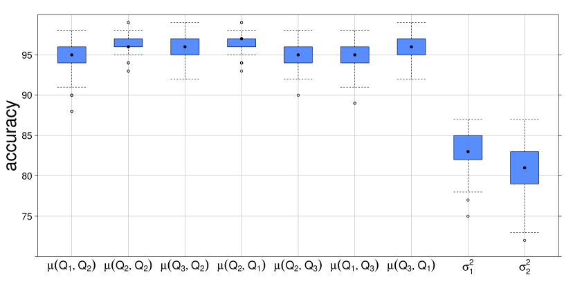
Figure 2: Side-by-side boxplots of accuracy values for MFVB against an MCMC benchmark for the Poisson response model (11).

The parameters on the horizontal axis of Figure 2 represent the estimated approximate posterior density functions for $\mu(x_{1},x_{2})$, evaluated at the quartiles of $x_{1}$ and $x_{2}$, and the estimated approximate posterior density functions for $\sigma_{1}^{2}$ and $\sigma_{2}^{2}$. The boxplots indicate that the accuracies for $\mu(x_{1},x_{2})$ are around 95%, while values between 80% and 85% are obtained for the variances $\sigma_{1}^{2}$ and $\sigma_{2}^{2}$.

Figure 3 shows the MFVB-based approximate posterior density functions against the MCMC result for a single replicated data-set. The accuracy of MFVB is particularly excellent for the $\mu(x_{1},x_{2})$ approximate posterior density functions.

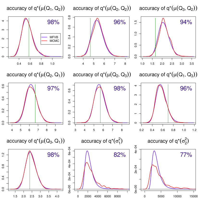
Figure 3: Approximate posterior density functions for Poisson response model (11). Vertical lines indicate the true values.

Figure 4 displays side-by-side boxplots of the accuracies for the 100 data-sets generated according to the Negative Binomial response model (12).

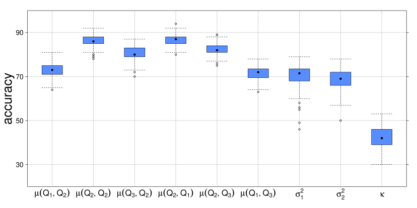
Figure 4: Side-by-side boxplots of accuracy values for MFVB against an MCMC benchmark for Negative Binomial response model (12).

The parameters on the horizontal axis in Figure 4 have similar meanings as in Figure 2, but the result for the approximate posterior density function of $\kappa$ is also included. Compared to the results for the Poisson case the accuracies for the Negative Binomial response model are lower, but still attain good performance for $\mu(x_{1},x_{2})$ with approximately values between 70 and 90%. The majority of the accuracies for the variances $\sigma_{1}^{2}$ and $\sigma_{2}^{2}$ is around 70%, while lower accuracies are obtained for $\kappa$.

Finally, Figure 5 compares the approximate posterior density functions obtained using MFVB inference and the MCMC result for a single replicated data-set. MFVB attains particularly good accuracies for the $\mu(x_{1},x_{2})$ approximate posterior density functions.

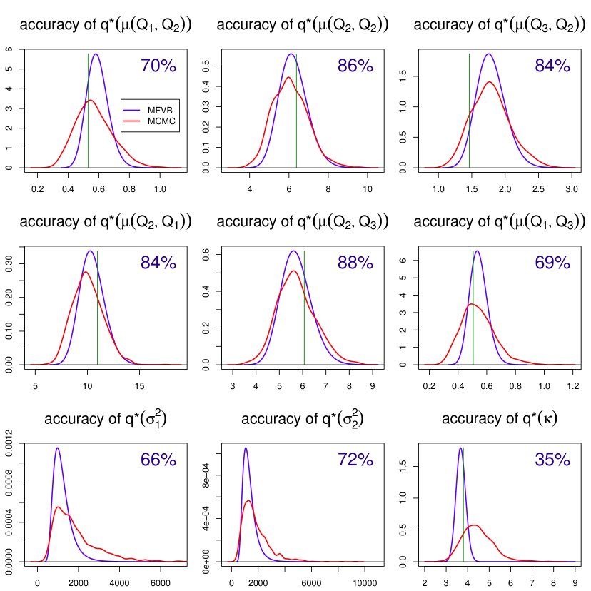
Figure 5: Approximate posterior density functions for Negative Binomial response model (12). Vertical lines indicate the true values.

6.1.2 Computational cost

Table 2 summarizes the computation times for MCMC and MFVB fitting in case of the Poisson and Negative Binomial experiment as run using an Intel Core i7-2760QM 2.40 GHz processor with 8 GBytes of random access memory. The average computing time for MFVB is considerably lower than that of MCMC. Nevertheless, the speed gains of MFVB need to be traded off against accuracy losses as shown in Figures 2 and 4.

	MCMC	MFVB
Poisson response model	856.66 (23.13)	2.24 (0.30)
Negative Binomial response model	1127.96 (56.73)	20.85 (3.52)

Table 2: Average (standard deviation) times in seconds for MCMC and MFVB inference based on the simulation study.

6.2 Applications

We now present some applications involving each of models (3) and (4) in turn.

6.2.1 North African Conflict

We fitted the Poisson response model (3) using Algorithm 1 to a data-set extracted from the Global Database of Events, Language and Tone (Leetaru & Schrodt, 2013). This database contains more than 200 million geo-located events, obtained from news reports, with global coverage between early 1979 and June 2012. For this example we extracted the daily number of material conflicts for each African country for the period September 2010 to June 2012. Our model is

$$\texttt{conflicts}_{ij}|\,\boldsymbol{\beta},\boldsymbol{u}_{1},U_{i}\stackrel{{\scriptstyle{\tiny\mbox{ind.}}}}{{\sim}}\mbox{Poisson}(\exp\{\beta_{0}+f_{1}(\texttt{time}_{j})+U_{i}\}),$$

with $\texttt{conflicts}_{ij}$ the number of news reports about material conflicts for country $i$ on date $j$, $\texttt{time}_{j}$ the time in days for date $j$ starting from September 1, 2010 and $U_{i}$ the random intercept for country $i$, $1\leq i\leq 54$. The total number of observations for all African countries is $n=36126$. Note that 20 spline basis functions were used for modeling $f_{1}$.

Figure 6 shows the estimate for $\exp\{\beta_{0}+f_{1}(\texttt{time}_{j})\}$ and corresponding 95% pointwise credible sets. The strong increase, starting around December 2010, in number of news reports about material conflicts coincides with the Arab Spring demonstrations and civil wars which took place in several African countries as Mauritania, Western Sahara, Morocco, Algeria, Tunisia, Libya, Egypt, Sudan, Djibouti and the related crisis in Mali. In addition, 95% credible sets for the estimates of $\exp(U_{i})$ are plotted for the fifteen countries with the largest random intercept estimates, i.e. showing larger numbers of material conflict-related news reports. Fitting using Algorithm 1 took $7$ minutes and $30$ seconds.

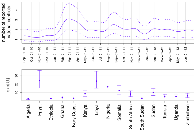
Figure 6: Poisson regression result using MFVB inference for global data on events, location and tone database. The solid curve in the top panel are posterior means and the dashed curves are pointwise 95% credible sets. The lower panel shows 95% credible sets for the estimates of $\exp(U_{i})$ for the fifteen countries with highest posterior means.

6.2.2 Adduct data

Illustrations of Negative Binomial semiparametric regression models have previously been given in Thurston, Wand & Weincke (2000) and Marley & Wand (2010) using data on adducts counts, which are carcinogen-DNA complexes, and smoking variables for 78 former smokers in the lung cancer study (Wiencke et al., 1999). Here we use Algorithm 1 to fit a version of the Bayesian penalized model that Marley & Wand (2010) fitted via MCMC.

Thurston, Wand & Weincke (2000) and Marley & Wand (2010) considered Negative Binomial additive models of the form:

$$\begin{array}[]{rcl}\texttt{adducts}_{i}|\,\boldsymbol{\beta},\boldsymbol{u}_{1},\boldsymbol{u}_{2},\boldsymbol{u}_{3},\boldsymbol{u}_{4},\kappa&\stackrel{{\scriptstyle{\tiny\mbox{ind.}}}}{{\sim}}&\mbox{Negative-Binomial}(\exp\{\beta_{0}+f_{1}(\texttt{ageInit}_{i})\\[8.61108pt] &&+f_{2}(\texttt{yearsSmoking}_{i})+f_{3}(\texttt{yearsSinceQuit}_{i})\\[8.61108pt] &&+f_{4}(\texttt{cigsPerDay}_{i})\},\kappa),\end{array}$$ (14)

with $\texttt{ageInit}_{i}$ the age of smoking initiation, $\texttt{yearsSmoking}_{i}$ the number of years of smoking, $\texttt{yearsSinceQuit}_{i}$ the number of years since quitting and $\texttt{cigsPerDay}_{i}$ the number of cigarettes smoked per day for subject $i$. The $f_{\ell}$, $1\leq\ell\leq 4$, are modelled using mixed-model based penalized splines as in (13), with 20 basis functions each.

Figure 7 displays the fitted functions for model (14). Marley & Wand (2010) reported slow MCMC convergence for this model, so we used burn-in size of 1000000 a retained sample size of 500000, and a thinning factor of 50 The MCMC-based fits are added as a reference to Figure 7.

Fitting of (14) via Algorithm 1 took 2 minutes whilst MCMC fitting in BUGS took 1 hour and 28 minutes. As indicated by Figure 7, the much faster MFVB estimates are quite close to the more accurate MCMC estimates.

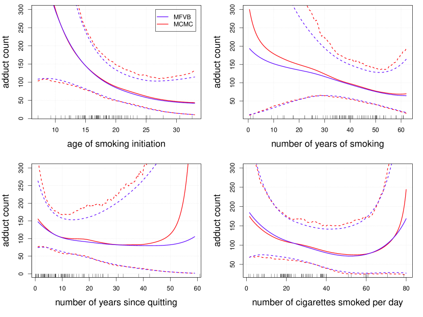
Figure 7: Negative Binomial regression result using MFVB and MCMC inference for adduct data set. Solid curves are posterior means for fitted functions while dashed curves are corresponding pointwise 95% credible sets.

6.3 Real-time Poisson Nonparametric Regression Movie

The web-site realtime-semiparametric-regression.net contains a movie that illustrates Algorithm 2 in the special case of Poisson nonparametric regression with $r=1$ The spline basis functions set-up is analogous to that given in (13).

The data are simulated according to

$$x_{\mbox{{\tiny\mbox{new}}}}\sim\mbox{Uniform}(0,1),\quad y_{\mbox{\tiny\mbox{new}}}|x_{\mbox{{\tiny\mbox{new}}}}\sim\mbox{Poisson}[\exp\{\cos(4\pi x_{\mbox{{\tiny\mbox{new}}}})+2\,x_{\mbox{{\tiny\mbox{new}}}}\}]$$

and the warm-up sample size is $n_{\mbox{\scriptsize warm}}=100$. The movie is under the link titled Poisson nonparametric regression. and shows the efficacy of Algorithm 2 for recovery of the underlying mean function in real time.

Appendix: Derivation of $q^{*}$ density functions

Derivation of $q^{*}(a_{\ell})$ and $q^{*}(\sigma^{2}_{\ell})$ for the Poisson and Negative Binomial response model

Standard manipulations lead to the following full conditional distributions:

$$\begin{array}[]{l}a_{\ell}|\text{rest}\stackrel{{\scriptstyle{\tiny\mbox{ind.}}}}{{\sim}}\mbox{Inverse-Gamma}(1,\sigma_{\ell}^{-2}+A_{\ell}^{-2})\ \ \text{and}\\[12.91663pt] \sigma^{2}_{\ell}|\text{rest}\stackrel{{\scriptstyle{\tiny\mbox{ind.}}}}{{\sim}}\mbox{Inverse-Gamma}(1/2\,(K_{\ell}+1),a^{-1}_{\ell}+1/2\,\|\boldsymbol{u}_{\ell}\|^{2}).\end{array}$$

Derivation of the $(\boldsymbol{\mu}_{q(\boldsymbol{\beta},\boldsymbol{u})},\boldsymbol{\Sigma}_{q(\boldsymbol{\beta},\boldsymbol{u})})$ updates for the Poisson response model

Adaptation of the derivations in Appendix A.3 of Wand (2013) leads to

$$E_{q}\left[\log p(\boldsymbol{y},\boldsymbol{\beta},\boldsymbol{u},\sigma^{2}_{1},\ldots,\sigma^{2}_{r},a_{1},\ldots,a_{r})\right] = E_{q}\bigg{[}\log\,p(\boldsymbol{y}|\boldsymbol{\beta},\boldsymbol{u})+\log\,p(\boldsymbol{\beta},\boldsymbol{u}|\sigma^{2}_{1},\ldots,\sigma^{2}_{r})$$

$$+\sum_{\ell=1}^{r}\log\,p(\sigma_{\ell}^{2}|a_{\ell})+\sum_{\ell=1}^{r}\log\,p(a_{\ell})\bigg{]}$$

$$= S+\mbox{terms not involving $\boldsymbol{\mu}_{q(\boldsymbol{\beta},\boldsymbol{u})}$ or $\boldsymbol{\Sigma}_{q(\boldsymbol{\beta},\boldsymbol{u})}$}$$

where

$$S \equiv \boldsymbol{y}^{T}\boldsymbol{C}\boldsymbol{\mu}_{q(\boldsymbol{\beta},\boldsymbol{u})}-\boldsymbol{1}^{T}\exp\left\{\boldsymbol{C}\boldsymbol{\mu}_{q(\boldsymbol{\beta},\boldsymbol{u})}+{\textstyle{\frac{1}{2}}}\mbox{diagonal}(\boldsymbol{C}\boldsymbol{\Sigma}_{q(\boldsymbol{\beta},\boldsymbol{u})}\boldsymbol{C}^{T})\right\}$$

$$-{\textstyle{\frac{1}{2}}}\mbox{tr}\left(\mbox{blockdiag}(\sigma_{\beta}^{-2}\boldsymbol{I}_{p},\mu_{q(1/\sigma_{1}^{2})}\boldsymbol{I}_{K_{1}},\ldots,\mu_{q(1/\sigma_{r}^{2})}\boldsymbol{I}_{K_{r}})\{\boldsymbol{\mu}_{q(\boldsymbol{\beta},\boldsymbol{u})}\boldsymbol{\mu}_{q(\boldsymbol{\beta},\boldsymbol{u})}^{T}+\boldsymbol{\Sigma}_{q(\boldsymbol{\beta},\boldsymbol{u})}\}\right)$$

$$-{\textstyle{\frac{1}{2}}}P\log(2\pi)-{\textstyle{\frac{1}{2}}}\,p\log(\sigma_{\beta}^{2})-{\textstyle{\frac{1}{2}}}\,\sum_{\ell=1}^{r}K_{\ell}\,E_{q}\{\log(\sigma_{\ell}^{2})\}-\boldsymbol{1}^{T}\log(\boldsymbol{y}!).$$

Then,

$$d_{\boldsymbol{\mu}_{q(\boldsymbol{\beta},\boldsymbol{u})}}\,S = \Big{(}\left[\boldsymbol{y}-\exp\{\boldsymbol{C}\boldsymbol{\mu}_{q(\boldsymbol{\beta},\boldsymbol{u})}+{\textstyle{\frac{1}{2}}}\mbox{diagonal}(\boldsymbol{C}\boldsymbol{\Sigma}_{q(\boldsymbol{\beta},\boldsymbol{u})}\boldsymbol{C}^{T})\}\right]^{T}\boldsymbol{C}$$

$$-\boldsymbol{\mu}_{q(\boldsymbol{\beta},\boldsymbol{u})}^{T}\mbox{blockdiag}(\sigma_{\beta}^{-2}\boldsymbol{I}_{p},\mu_{q(1/\sigma_{1}^{2})}\boldsymbol{I}_{K_{1}},\ldots,\mu_{q(1/\sigma_{r}^{2})}\boldsymbol{I}_{K_{r}})\Big{)}d\boldsymbol{\mu}_{q(\boldsymbol{\beta},\boldsymbol{u})}$$

and by Theorem 6, Chapter 5, of Magnus & Neudecker (1999),

$$\{{\sf D}_{\boldsymbol{\mu}_{q(\boldsymbol{\beta},\boldsymbol{u})}}\,S\}^{T} = \boldsymbol{C}^{T}\left[\,\boldsymbol{y}-\exp\{\boldsymbol{C}\boldsymbol{\mu}_{q(\boldsymbol{\beta},\boldsymbol{u})}+{\textstyle{\frac{1}{2}}}\mbox{diagonal}(\boldsymbol{C}\boldsymbol{\Sigma}_{q(\boldsymbol{\beta},\boldsymbol{u})}\boldsymbol{C}^{T})\}\right]$$

$$-\mbox{blockdiag}(\sigma_{\beta}^{-2}\boldsymbol{I}_{p},\mu_{q(1/\sigma_{1}^{2})}\boldsymbol{I}_{K_{1}},\ldots,\mu_{q(1/\sigma_{r}^{2})}\boldsymbol{I}_{K_{r}})\boldsymbol{\mu}_{q(\boldsymbol{\beta},\boldsymbol{u})}.$$

Next,

$$d_{\mbox{vec}(\boldsymbol{\Sigma}_{q(\boldsymbol{\beta},\boldsymbol{u})})}\,S = -{\textstyle{\frac{1}{2}}}\mbox{vec}\Big{(}\boldsymbol{C}^{T}\mbox{diag}[\exp\{\boldsymbol{C}\boldsymbol{\mu}_{q(\boldsymbol{\beta},\boldsymbol{u})}+{\textstyle{\frac{1}{2}}}\mbox{diagonal}(\boldsymbol{C}\boldsymbol{\Sigma}_{q(\boldsymbol{\beta},\boldsymbol{u})}\boldsymbol{C}^{T})\}]\boldsymbol{C}$$

$$+\mbox{blockdiag}(\sigma_{\beta}^{-2}\boldsymbol{I}_{p},\mu_{q(1/\sigma_{1}^{2})}\boldsymbol{I}_{K_{1}},\ldots,\mu_{q(1/\sigma_{r}^{2})}\boldsymbol{I}_{K_{r}})\Big{)}^{T}d\,\mbox{vec}(\boldsymbol{\Sigma}_{q(\boldsymbol{\beta},\boldsymbol{u})})$$

and

$$\mbox{vec}^{-1}\left(({\sf D}_{\mbox{vec}(\boldsymbol{\Sigma}_{q(\boldsymbol{\beta},\boldsymbol{u})})}\,S)^{T}\right) = -{\textstyle{\frac{1}{2}}}(\boldsymbol{C}^{T}\mbox{diag}[\,\exp\{\boldsymbol{C}\boldsymbol{\mu}_{q(\boldsymbol{\beta},\boldsymbol{u})}+{\textstyle{\frac{1}{2}}}\mbox{diagonal}(\boldsymbol{C}\boldsymbol{\Sigma}_{q(\boldsymbol{\beta},\boldsymbol{u})}\boldsymbol{C}^{T})\}]\,\boldsymbol{C}$$

$$+\mbox{blockdiag}(\sigma_{\beta}^{-2}\boldsymbol{I}_{p},\mu_{q(1/\sigma_{1}^{2})}\boldsymbol{I}_{K_{1}},\ldots,\mu_{q(1/\sigma_{r}^{2})}\boldsymbol{I}_{K_{r}})).$$

The final result follows from plugging in $\{{\sf D}_{\boldsymbol{\mu}_{q(\boldsymbol{\beta},\boldsymbol{u})}}\,S\}^{T}$ and $\mbox{vec}^{-1}\left(({\sf D}_{\mbox{vec}(\boldsymbol{\Sigma}_{q(\boldsymbol{\beta},\boldsymbol{u})})}\,S)^{T}\right)$ in the updating formulas (LABEL:eq:updatesMatt).

Derivation of $q^{*}(g_{i})$ and $q^{*}(\kappa)$ for the Negative Binomial response model

Standard manipulations lead to the following full conditional distribution

$$\begin{array}[]{l}g_{i}|\text{rest}\stackrel{{\scriptstyle{\tiny\mbox{ind.}}}}{{\sim}}\mbox{Gamma}(\kappa+y_{i},1+\kappa\exp\{-\boldsymbol{c}_{i}^{T}[\boldsymbol{\beta}^{T}\ \boldsymbol{u}^{T}]^{T}\})\end{array}$$

such that $q^{*}(g_{i})$ is the Gamma density function specified in (9). In addition, standard distributional results for the Gamma density function lead to

$$\begin{array}[]{ll}\boldsymbol{\mu}_{q(\log(\boldsymbol{g}))}=&\text{digamma}(\boldsymbol{1}\mu_{q(\kappa)}+\boldsymbol{y})-\log(\boldsymbol{1}+\mu_{q(\kappa)}\exp\{-\boldsymbol{C}\boldsymbol{\mu}_{q(\boldsymbol{\beta},\boldsymbol{u})}\\[8.61108pt] &+\frac{1}{2}\,\mbox{diagonal}(\boldsymbol{C}\boldsymbol{\Sigma}_{q(\boldsymbol{\beta},\boldsymbol{u})}\boldsymbol{C}^{T})\}).\end{array}$$

The density function $q^{*}(\kappa)$ can be obtained by adapting the expressions in Appendix A.1 of Wand et al. (2011) and result in

$$\mu_{q(\kappa)}=\exp\left[\log\left\{\mathcal{H}(1,n,C_{1},\kappa_{\text{min}},\kappa_{\text{max}})\right\}-\log\left\{\mathcal{H}(0,n,C_{1},\kappa_{\text{min}},\kappa_{\text{max}})\right\}\right].$$

Derivation of the $(\boldsymbol{\mu}_{q(\boldsymbol{\beta},\boldsymbol{u})},\boldsymbol{\Sigma}_{q(\boldsymbol{\beta},\boldsymbol{u})})$ updates for the Negative Binomial response model

Note that

$$E_{q}[\log p(\boldsymbol{y},\boldsymbol{g},\boldsymbol{\beta},\boldsymbol{u},\kappa,\sigma^{2}_{1},\ldots,\sigma^{2}_{r},a_{1},\ldots,a_{r})] = E_{q}\bigg{[}\log\,p(\boldsymbol{y}|\boldsymbol{g})+\log\,p(\boldsymbol{g}|\boldsymbol{\beta},\boldsymbol{u},\kappa)$$

$$+\log\,p(\boldsymbol{\beta},\boldsymbol{u}|\sigma^{2}_{1},\ldots,\sigma^{2}_{r})+\log\,p(\kappa)$$

$$+\sum_{\ell=1}^{r}\log\,p(\sigma_{\ell}^{2}|a_{\ell})+\sum_{\ell=1}^{r}\log\,p(a_{\ell})\bigg{]}$$

$$= S+\mbox{terms not involving $\boldsymbol{\mu}_{q(\boldsymbol{\beta},\boldsymbol{u})}$ or $\boldsymbol{\Sigma}_{q(\boldsymbol{\beta},\boldsymbol{u})}$}$$

where

$$\begin{array}[]{lll}S&\equiv&nE_{q}[\kappa\log\left(\kappa\right)]-\mu_{q(\kappa)}\boldsymbol{1}^{T}\boldsymbol{C}\boldsymbol{\mu}_{q(\boldsymbol{\beta},\boldsymbol{u})}-nE_{q}[\log\left(\Gamma(\kappa)\right)]+(\mu_{q(\kappa)}-1)\boldsymbol{1}^{T}E_{q}[\log\left(\boldsymbol{g}\right)]\\[8.61108pt] &&-\mu_{q(\kappa)}\boldsymbol{\mu}^{T}_{q(\boldsymbol{g})}\exp\{-\boldsymbol{C}\boldsymbol{\mu}_{q(\boldsymbol{\beta},\boldsymbol{u})}+{\textstyle{\frac{1}{2}}}\mbox{diagonal}(\boldsymbol{C}\boldsymbol{\Sigma}_{q(\boldsymbol{\beta},\boldsymbol{u})}\boldsymbol{C}^{T})\}\\[8.61108pt] &&-{\textstyle{\frac{1}{2}}}\mbox{tr}\left(\mbox{blockdiag}(\sigma_{\beta}^{-2}\boldsymbol{I}_{p},\mu_{q(1/\sigma_{1}^{2})}\boldsymbol{I}_{K_{1}},\ldots,\mu_{q(1/\sigma_{r}^{2})}\boldsymbol{I}_{K_{r}})\{\boldsymbol{\mu}_{q(\boldsymbol{\beta},\boldsymbol{u})}\boldsymbol{\mu}_{q(\boldsymbol{\beta},\boldsymbol{u})}^{T}+\boldsymbol{\Sigma}_{q(\boldsymbol{\beta},\boldsymbol{u})}\}\right)\\[8.61108pt] &&-{\textstyle{\frac{1}{2}}}P\log(2\pi)-{\textstyle{\frac{1}{2}}}\,p\log(\sigma_{\beta}^{2})-{\textstyle{\frac{1}{2}}}\,\sum_{\ell=1}^{r}K_{\ell}\,E_{q}\{\log(\sigma_{\ell}^{2})\}.\end{array}$$

Then,

$$\{{\sf D}_{\boldsymbol{\mu}_{q(\boldsymbol{\beta},\boldsymbol{u})}}\,S\}^{T} = \mu_{q(\kappa)}\boldsymbol{C}^{T}\left[\,\boldsymbol{\mu}_{q(\boldsymbol{g})}\odot\exp\{-\boldsymbol{C}\boldsymbol{\mu}_{q(\boldsymbol{\beta},\boldsymbol{u})}+{\textstyle{\frac{1}{2}}}\mbox{diagonal}(\boldsymbol{C}\boldsymbol{\Sigma}_{q(\boldsymbol{\beta},\boldsymbol{u})}\boldsymbol{C}^{T})\}-\boldsymbol{1}\right]$$

$$-\mbox{blockdiag}(\sigma_{\beta}^{-2}\boldsymbol{I}_{p},\mu_{q(1/\sigma_{1}^{2})}\boldsymbol{I}_{K_{1}},\ldots,\mu_{q(1/\sigma_{r}^{2})}\boldsymbol{I}_{K_{r}})\boldsymbol{\mu}_{q(\boldsymbol{\beta},\boldsymbol{u})}$$

and

$$d_{\mbox{vec}(\boldsymbol{\Sigma}_{q(\boldsymbol{\beta},\boldsymbol{u})})}\,S = -{\textstyle{\frac{1}{2}}}\mbox{vec}\Big{(}\mu_{q(\kappa)}\boldsymbol{C}^{T}\mbox{diag}[\boldsymbol{\mu}_{q(\boldsymbol{g})}\odot\exp\{-\boldsymbol{C}\boldsymbol{\mu}_{q(\boldsymbol{\beta},\boldsymbol{u})}$$

$$+{\textstyle{\frac{1}{2}}}\mbox{diagonal}(\boldsymbol{C}\boldsymbol{\Sigma}_{q(\boldsymbol{\beta},\boldsymbol{u})}\boldsymbol{C}^{T})\}]\boldsymbol{C}$$

$$+\mbox{blockdiag}(\sigma_{\beta}^{-2}\boldsymbol{I}_{p},\mu_{q(1/\sigma_{1}^{2})}\boldsymbol{I}_{K_{1}},\ldots,\mu_{q(1/\sigma_{r}^{2})}\boldsymbol{I}_{K_{r}})\Big{)}^{T}d\,\mbox{vec}(\boldsymbol{\Sigma}_{q(\boldsymbol{\beta},\boldsymbol{u})})$$

such that

$$\mbox{vec}^{-1}\left(({\sf D}_{\mbox{vec}(\boldsymbol{\Sigma}_{q(\boldsymbol{\beta},\boldsymbol{u})})}\,S)^{T}\right) = -{\textstyle{\frac{1}{2}}}(\mu_{q(\kappa)}\boldsymbol{C}^{T}\mbox{diag}[\boldsymbol{\mu}_{q(\boldsymbol{g})}\odot\exp\{-\boldsymbol{C}\boldsymbol{\mu}_{q(\boldsymbol{\beta},\boldsymbol{u})}$$

$$+{\textstyle{\frac{1}{2}}}\mbox{diagonal}(\boldsymbol{C}\boldsymbol{\Sigma}_{q(\boldsymbol{\beta},\boldsymbol{u})}\boldsymbol{C}^{T})\}]\,\boldsymbol{C}$$

$$+\mbox{blockdiag}(\sigma_{\beta}^{-2}\boldsymbol{I}_{p},\mu_{q(1/\sigma_{1}^{2})}\boldsymbol{I}_{K_{1}},\ldots,\mu_{q(1/\sigma_{r}^{2})}\boldsymbol{I}_{K_{r}})).$$

The final result follows from plugging in these expressions in the updating formulas (LABEL:eq:updatesMatt).

References

• Albert &ย Chib (1993) Albert, JH &ย Chib, S (1993). โ€˜Bayesian analysis of binary and polychotomous response dataโ€™, Journal of the American Statistical Association, 88, 669โ€“679.
• Consonni &ย Marin (2007) Consonni, G &ย Marin, J-M (2007). โ€˜Mean-field variational approximate Bayesian inference for latent variable modelsโ€™, Computational Statistics and Data Analysis, 52, 790โ€“798.
• Girolami & Rogers (2006) Girolami, M. &ย Rogers, S. (2006). โ€˜Variational Bayesian multinomial probit regressionโ€™, Neural Computation, 18, 1790โ€“1817.
• Jaakkola & Jordan (2000) Jaakkola, TS &ย Jordan, MI (2000). โ€˜Bayesian parameter estimation via variational methodsโ€™, Statistics and Computing 10, 25โ€“37.
• Knowles & Minka (2011) Knowles, DA & Minka, TP (2011), โ€˜Non-conjugate message passing for multinomial and binary regressionโ€™, In J. Shawe-Taylor, R.S. Zamel, P. Bartlett, F. Pereira and K.Q. Weinberger, editors, Advances in Neural Information Processing Systems, 24, 1701โ€“1709.
• Lawless (1987) Lawless, JF (1987), โ€˜Negative Binomial and mixed Poisson regressionโ€™, Canadian Journal of Statistics, 15, 209โ€“225.
• Leetaru & Schrodt (2013) Leetaru, KH & Schrodt, PA (2013), โ€˜A 30-year georeferenced global event database: The Global Database of Events, Language, and Tone (GDELT)โ€™, International Studies Association Conference, April 2013, San Francisco, USA.