Electric charge susceptibility in 2+1 flavour QCD on an anisotropic lattice

Abstract:

The FASTSUM Collaboration presents its first results for the electric charge susceptibility in QCD using $2+1$ dynamical flavours of Wilson quark on anisotropic lattices. Spatial volumes of $(2.94\ \mbox{fm})^{3}$ are used at fixed cut-off with temperatures ranging from below $T_{c}$ to $\sim 2T_{c}$.

1 Introduction

The measurement of fluctuations of conserved charges can probe both the thermal state of the medium and its critical behaviour. The fluctuations are quantified by the susceptibilities, defined as second (and higher) derivatives of the free energy with respect to the chemical potential associated with the investigated charge. In QCD, taking into account the three light flavours, usually three charges are studied in the literature: baryon number, electric charge, strangeness. Their susceptibilities probe the actual degrees of freedom that carry such charges, i.e. quarks or their bound states.

QCD shows a very interesting phase structure [1]. The main characteristic, at zero baryon chemical potential ($\mu_{B}$), is a crossover transition from a confined, chirally broken phase at low temperature ($T$) to a deconfined, chirally symmetric phase at high temperature called quark-gluon plasma (QGP) around $T_{c}\approx 150$MeV. Fluctuations can be used to probe quark deconfinement [2] by studying event-by-event fluctuations of charged particle ratios [3]. Susceptibilities show a rapid rise in the crossover region: at low temperature they are small since quarks are confined; at high temperature they are large and they approach the ideal gas limit.

There are many specific reasons why physicists are interested in studying these quantities; here we recall the following:

• the QCD transition is today reproduced in the heavy ion collision experiments at BNL (RHIC) and at CERN (LHC) where the fluctuations can be studied [4]: it is clearly very important for our understanding of the strong interaction to compare their measurements with lattice QCD determinations;

• susceptibilities can be seen as coefficients of the Taylor expansion of the free energy with respect to the chemical potentials; in this form they can be used to perform numerical studies at finite density QCD [5, 6];

• QCD may have a critical point, an endpoint of a line of first order phase transitions which extends from the $\mu_{B}$-axis into the ($\mu_{B}$,$T$) plane. Susceptibilities can probe its presence and, in particular, the baryon number susceptibility is expected to diverge at the critical point. Its position can be estimated studying the radius of convergence [7] of the Taylor series introduced in the previous paragraph;

• the susceptibilities of the conserved charges enter the study of the transport properties of the QGP via Kubo formulae [8], e.g. the electric charge susceptibility $\chi_{Q}$ connects the charge diffusion coefficient $D$ with the electrical conductivity $\sigma$: $\sigma=\chi_{Q}D$.

Among the available theoretical tools, lattice calculations are probably the best for calculating the properties of QGP and in particular the susceptibilities from first principles: this approach is followed in this work. Nearly all lattice studies of susceptibilities have so far been carried out using staggered fermions. In this study we employ instead clover-improved Wilson fermions (for an earlier study using Wilson fermions see Ref. [9]).

2 Simulation details

The action that we have used is, for the gauge sector, Symanzik-improved with tree-level tadpole-improved coefficients and for the fermion sector, a $2+1$ flavour anisotropic clover action with stout-link smearing; for details see Ref. [10]. The configurations have been generated using the Chroma Library [11] on IBM Blue Gene/P and Blue Gene/Q supercomputers.

The volumes we have used are $24^{3}\times N_{t}$, where the values of $N_{t}$, together with the corresponding temperature and the number of configurations generated, are given in Table 1.

$N_{t}$	40	36	32	28	24	20	16
$T$ [MeV]	141	156	176	201	235	281	352
$N_{\text{cfg}}$	500	500	1000	1000	1000	1000	1000

Table 1: Some simulation parameters.

We used anisotropic lattices with a physical anisotropy $\xi\equiv a_{s}/a_{t}=3.5$: the temporal lattice spacing, measured using $M_{\Omega}$ to set the scale, is $a_{t}=0.03506(23)$ fm ($a_{t}^{-1}=5.63(4)$ GeV) and $a_{s}=0.1227(8)$ fm; for details see Ref. [12]. Moreover, $M_{\pi}/M_{\rho}=0.446(3)$ and $M_{\pi}=392(4)$ MeV, i.e. 2.9 times bigger than the physical value.

3 Definitions and observables

Introducing the quark chemical potentials $\mu_{u},\mu_{d},\mu_{s}$ and the charges $q^{u}=+\frac{2}{3}$, $q^{d}=q^{s}=-\frac{1}{3}$, for each flavour (we use also here the correspondence: $1\leftrightarrow$up, $2\leftrightarrow$down, $3\leftrightarrow$strange and also in the following $l\rightarrow$ light, $s\rightarrow$ strange) we define the following quantities:

• quark number densities: $n_{i}=\frac{T}{V}\frac{\partial\ln{Z}}{\partial\mu_{i}}$;

• quark number susceptibilities: $\chi_{ij}=\frac{T}{V}\frac{\partial^{2}\ln{Z}}{\partial\mu_{i}\partial\mu_{j}}$.

Introducing the electric charge chemical potential $\mu_{Q}$, the electric charge $Q$ and its susceptibility $\chi_{Q}$ are given by:

$$Q=\frac{T}{V}\frac{\partial\ln{Z}}{\partial\mu_{Q}}=\sum_{i=1}^{3}q^{i}n_{i}\ ,\quad\quad\chi_{Q}=\frac{\partial Q}{\partial\mu_{Q}}=\sum_{i=1}^{3}(q^{i})^{2}\chi_{ii}+\sum_{i\neq j}^{3}q^{i}q^{j}\chi_{ij}.$$ (1)

We now introduce the following terms ($M$ is the fermion matrix):

$$T_{1}^{i}=\langle\frac{T}{V}\mbox{Tr}{\left[M^{-1}\frac{\partial M}{\partial\mu_{i}}\right]}\rangle\ ,\quad T_{2}^{i}=\langle\frac{T}{V}\mbox{Tr}{\left[M^{-1}\frac{\partial^{2}M}{\partial\mu_{i}^{2}}\right]}\rangle\ ,$$

$$T_{3}^{ij}=\langle\frac{T}{V}\mbox{Tr}{\left[M^{-1}\frac{\partial M}{\partial\mu_{i}}\right]}\mbox{Tr}{\left[M^{-1}\frac{\partial M}{\partial\mu_{j}}\right]}\rangle\ ,\quad T_{4}^{i}=\langle\frac{T}{V}\mbox{Tr}{\left[M^{-1}\frac{\partial M}{\partial\mu_{i}}M^{-1}\frac{\partial M}{\partial\mu_{i}}\right]}\rangle\ ,$$ (2)

which we can be used to determine the quantities:

$$n_{i} = T_{1}^{i}\ ;$$ (3)

$$\chi_{ii} = -(T_{1}^{i})^{2}+T_{2}^{i}+T_{3}^{ii}-T_{4}^{i}\ ;$$ (4)

$$\chi_{ij} = -T_{1}^{i}T_{1}^{j}+T_{3}^{ij}\quad\mbox{(here $i\neq j$)}\ .$$ (5)

Note that $T_{1}^{i}=0$ for zero chemical potentials, in fact $n_{i}=0$ and $Q=0$; therefore there is no need to compute this quantity numerically.

The simplest quantity we can determine is the isospin susceptibility (defining $\mu_{I}=\mu_{d}-\mu_{u}$):

$$\chi_{I}=\frac{T}{V}\frac{\partial^{2}\ln{Z}}{\partial\mu_{I}^{2}}=\frac{1}{4}\frac{T}{V}\left[\frac{\partial^{2}\ln{Z}}{\partial\mu_{u}^{2}}+\frac{\partial^{2}\ln{Z}}{\partial\mu_{d}^{2}}-2\frac{\partial^{2}\ln{Z}}{\partial\mu_{u}\partial\mu_{d}}\right]=\frac{1}{4}\sum_{i=1}^{2}\left[T_{2}^{i}-T_{4}^{i}\right].$$ (6)

We note that it depends only on the terms $T_{2}$ and $T_{4}$ but not $T_{3}$ which, from a numerical point of view, is the most expensive quantity to determine since it comes from a disconnected diagram.

Below we compare our results at high temperature with the expressions for free massless fermions in the continuum limit, which read:

$$\chi_{I} \rightarrow \frac{T^{2}}{2};$$ (7)

$$\chi_{Q} \rightarrow T^{2}\sum_{i=1}^{3}q_{i}^{2}\ ,$$ (8)

where $\sum_{i=1}^{3}q_{i}^{2}=2/3$.

Moreover, we also compare the susceptibilities with those obtained from free Wilson fermions, which can be determined analytically starting from the following expression for the baryon density, valid for $N_{f}$ flavours and $N_{c}$ colours:

$$n^{free}_{B}(\mu)=\frac{8N_{f}N_{c}}{N_{s}^{3}N_{t}}\sum_{k_{4},k_{i}}\frac{iP_{4}\sin{(k_{4}+i\mu)}\left[1-2P_{s}\sum_{i}\cos{k_{i}}\right]}{\left[1-2P_{s}\sum_{i}\cos{k_{i}}-2P_{4}\cos{(k_{4}+i\mu)}\right]^{2}+4P_{s}^{2}\sum_{i}\sin^{2}{k_{i}}+4P_{4}^{2}\sin^{2}{(k_{4}+i\mu)}}\ ,$$

where $i=1,2,3$, $\ k_{i}$ are the discretised momenta, the coefficients $P_{4}$ and $P_{s}$ are given by:

$$P_{4}=\nu_{t}/(m+\nu_{t}+3/\gamma_{f})\ ,\quad P_{s}=\nu_{s}/\left[2\ \xi_{0}\ (m+\nu_{t}+3/\gamma_{f})\right],$$

and $\nu_{t}=1$, $\nu_{s}=\gamma_{g}/\gamma_{f}$ and $\xi_{0}=\gamma_{g}$ ($\gamma_{g}$ is the bare gauge anisotropy and $\gamma_{f}$ is the bare fermion anisotropy). Note that when we compare with our data, $\gamma_{f}$ has to be replaced with $\xi$, the physical value. This relation was determined following the approach discussed in Sec. 4.2.4 of Ref. [13].

4 A few technical aspects

We estimated the traces of Eq. (2) using $N_{v}$ noise vectors $\eta_{i}$; for connected terms, i.e. $T_{2},T_{4}$, we used just $N_{v}=9$ noise vectors but for the disconnected term, i.e. $T_{3}$, we used $N_{v}=200$ noise vectors for $N_{t}=40$ and $N_{v}=100$ for the others. As discussed in Ref. [14] the term $T_{3}$, which contain two traces, has a significantly larger variance than the other terms and therefore needs a larger number of random vectors. It is worth noting that in this case the standard error of the mean falls like the inverse of the number of noise vectors (not like the square root of it) so that increasing $N_{v}$ has an evident effect in the final result.

As discussed in Ref. [15] the most efficient way to determine the square of a trace is by the following relation:

$$(\mbox{Tr}{A})^{2}=\frac{2}{N_{v}(N_{v}-1)}\sum_{i>j=1}^{N_{v}}\eta^{\dagger}_{i}A\eta_{i}\ \eta^{\dagger}_{j}A\eta_{j}\ ,$$ (9)

i.e. the diagonal terms are not taken into account because they would introduce a bias in the final result given by a term whose relative significance is $O(1/N_{v})$.

We tested the effect of dilution [16, 17] in the colour and Dirac space but we did not see any improvement in the final results. A dilution test done with $N_{t}=40$ has brought the following results: we have noted a reduction of the errors in the real part of $T_{1}$ by a factor $\sim 2$, and in the imaginary part of $T_{2}$ by a factor $\sim 3$; in all other cases the effect of dilution has been counterproductive. This is not a surprise because dilution has a positive effect only if the off-diagonal elements of a matrix dominate the diagonal ones, therefore the effect depends strongly on the observable under consideration.

5 Results

In this Section we present our preliminary results. In Figure 1 (Left) we present the result for the isospin susceptibility, normalising it with respect to the continuum expectation at high temperature, Eq. (7). As can be seen for $T\gtrsim 270$MeV the value is systematically higher than the expected one, i.e. unity, for free massless fermions living in a continuum spacetime. This is a lattice artefact which is a consequence of combined effect of our fixed cut-off approach and the small number of effective sites in the temporal direction ($N_{t}/\xi=4.6,5.7,6.8,\ldots$). This is evident looking at the dashed-red line which shows the same quantity for free massless lattice fermions, i.e. taking into account the effect of discretisation of the spacetime.

In Figure 1 (Right) we compare directly the result with that of massless free Wilson fermions. Here the discretisation effects are clearly taken into account and for $T\gtrsim 250$MeV the value of $\chi_{I}$ is above 85% of the Stefan-Boltzmann value. In the figure we plot moreover the result with two values of the fermion anisotropy: the physical one, $\gamma_{f}=\xi=3.5$, and the bare one, $\gamma_{f}=3.4$. The importance of using the correct value for the parameter $\gamma_{f}$ to compare our results with the Stefan-Boltzmann limit is evident.

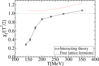
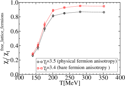
Figure 1: (Left) $\chi_{I}$ normalised using the high temperature expected behaviour (for free massless fermions living in a continuum spacetime). For comparison the same quantity for free massless lattice fermions is plotted. (Right) $\chi_{I}$ normalised with respect to the same quantity calculated for free massless lattice fermions using two values for the fermion anisotropy.

The contribution of the different terms to the susceptibilities are shown in Figure 2 (Left). We can see that the main contribution to the final value of the susceptibilities is given by the terms $T_{2}$ and $T_{4}$; note also the appreciable difference between the light and the strange quarks.

From Figure 2 (Left) we can see moreover the contribution of the disconnected term $T_{3}$. As discussed in Ref. [14] it is expected that this term is negative, basically as a consequence of hopping parameter expansion analysis. Hard thermal loop (HTL) perturbation theory showed a decade ago [19] that $\chi_{ij}=T_{3}^{ij}$ should be different from zero, showing a clear correlation between different flavours. Recent lattice calculations [18] have shown a clear dip for the off-diagonal term (in the crossover region). Our results, both for diagonal and off-diagonal contributions, show that it is compatible with zero, either at low and high temperature: this is probably a consequence of our relatively large pion mass.

The electric charge susceptibility is presented in Figure 2 (Right). Here we present this quantity normalised with respect to the high temperature behaviour expected for free massless fermions living in a continuum spacetime, Eq. (8). The cut-off effects are clearly present at high temperature as for Figure 1 (Left). The rapid rise of $\chi_{Q}$, signalling the transition from the confined phase to the deconfined phase, is evident around $T_{c}\sim 150$MeV.

In this preliminary figure, we have included all terms of Eq. (2) only for a few values of the temperature (see legend). Taking into account the results of Figure 2 (Left) and the fact that the disconnected contribution has had little effect at those temperatures where the electric charge susceptibility has been calculated, we can infer it will also have little affect for the other temperatures.

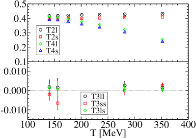
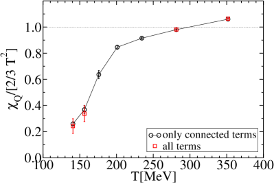
Figure 2: (Left) Terms $T_{2}$, $T_{4}$ and $T_{3}$. (Right) $\chi_{Q}$ normalised using the expected high temperature behaviour (for free massless fermions living in a continuum spacetime).

6 Conclusion and outlook

We have presented here our preliminary calculations of isospin and electric charge susceptibility in $2+1$ flavour QCD on anisotropic lattices using a fixed cut-off approach to explore a range of temperature which goes from below $T_{c}$ to $\sim 2T_{c}$. We are completing the determination of the susceptibilities on the volume $24^{3}$ on all the configurations at our disposal. When this is complete, we plan to combine these results with the measurement of the electrical conductivity, see Refs. [20], to determine the charge diffusion coefficient $D$. Moreover, by an appropriate combination of the terms of Eq. (2), we will determine the other relevant susceptibilities, in particular the one associated with the baryon number, $\chi_{B}$.

References

- [1] K. Fukushima and T. Hatsuda, Rept. Prog. Phys. 74 (2011) 014001 [arXiv:1005.4814 [hep-ph]].
- [2] M. Asakawa, U. W. Heinz and B. Muller, Phys. Rev. Lett. 85 (2000) 2072 [hep-ph/0003169].
- [3] M. Bleicher, S. Jeon and V. Koch, Phys. Rev. C 62 (2000) 061902 [hep-ph/0006201].
- [4] B. Abelev et al. [ALICE Collaboration], Phys. Rev. Lett. 110 (2013) 152301 [arXiv:1207.6068 [nucl-ex]].
- [5] C. R. Allton, M. Doring, S. Ejiri, S. J. Hands, O. Kaczmarek, F. Karsch, E. Laermann and K. Redlich, Phys. Rev. D 71 (2005) 054508 [hep-lat/0501030].
- [6] C. Miao et al. [RBC-Bielefeld Collaboration], PoS LATTICE 2008 (2008) 172 [arXiv:0810.0375 [hep-lat]].
- [7] R. V. Gavai and S. Gupta, Phys. Rev. D 78 (2008) 114503 [arXiv:0806.2233 [hep-lat]].
- [8] H. B. Meyer, Eur. Phys. J. A 47 (2011) 86 [arXiv:1104.3708 [hep-lat]].
- [9] S. Borsanyi, S. Durr, Z. Fodor, C. Hoelbling, S. D. Katz, S. Krieg, D. Nogradi and K. K. Szabo et al., JHEP 1208 (2012) 126 [arXiv:1205.0440 [hep-lat]].
- [10] R. G. Edwards, B. Joo and H. -W. Lin, Phys. Rev. D 78 (2008) 054501 [arXiv:0803.3960 [hep-lat]].
- [11] R. G. Edwards et al. [SciDAC and LHPC and UKQCD Collaborations], Nucl. Phys. Proc. Suppl. 140 (2005) 832 [hep-lat/0409003].
- [12] H. -W. Lin et al. [Hadron Spectrum Collaboration], Phys. Rev. D 79 (2009) 034502 [arXiv:0810.3588 [hep-lat]].
- [13] I. Montvay and G. Munster, Cambridge, UK: Univ. Pr. (1994) 491 p. (Cambridge monographs on mathematical physics).
- [14] S. A. Gottlieb, W. Liu, D. Toussaint, R. L. Renken and R. L. Sugar, Phys. Rev. Lett. 59 (1987) 2247; Phys. Rev. D 38 (1988) 2888.
- [15] R. V. Gavai, S. Gupta and P. Majumdar, Phys. Rev. D 65 (2002) 054506 [hep-lat/0110032].
- [16] W. Wilcox, hep-lat/9911013.
- [17] J. Foley, K. Jimmy Juge, A. O’Cais, M. Peardon, S. M. Ryan and J. -I. Skullerud, Comput. Phys. Commun. 172 (2005) 145 [hep-lat/0505023].
- [18] S. Borsanyi, Z. Fodor, S. D. Katz, S. Krieg, C. Ratti and K. Szabo, JHEP 1201 (2012) 138 [arXiv:1112.4416 [hep-lat]].
- [19] J. P. Blaizot, E. Iancu and A. Rebhan, Phys. Lett. B 523 (2001) 143 [hep-ph/0110369].
- [20] A. Amato, G. Aarts, C. Allton, P. Giudice, S. Hands and J. -I. Skullerud, arXiv:1307.6763 [hep-lat]; PoS LATTICE 2013 (2013) 176.