The local limit of unicellular maps in high genus

Abstract

We show that the local limit of unicellular maps whose genus is proportional to the number of edges is a supercritical geometric Galton-Watson tree conditioned to survive. The proof relies on enumeration results obtained via the recent bijection given by the second author together with Féray and Fusy.

1 Introduction

Recently, the last author of this note studied the large scale structure of random unicellular maps whose genus grows linearly with their size [11]. Our goal here is to identify explicitly the local limit of the latter as a super-critical geometric Galton-Watson tree conditioned to survive.

Motivated by the theory of two-dimensional quantum gravity, the study of local limits (also known as Benjamini-Schramm limits [4]) of random planar maps and graphs has been rapidly developing over the last years, since the introduction of the Uniform Infinite Planar Triangulation (UIPT) by Angel & Schramm [2]. The UIPT is defined as the local limit in distribution (see definition below) of uniform random triangulations of the sphere, when their size tends to infinity.

It is natural to expect (see [8]) that, for any fixed $g\geq 1$, the UIPT is also the local limit of uniform random triangulations of a surface of genus $g$ when their size tends to infinity (note that the situation is totally different for scaling limits, where the genus affects the topology of the limiting surface [5]). However, one expects to obtain a totally different picture if one lets the genus of the maps grow linearly with their size. In this case, the limiting average degree is strictly greater than in the planar case, so that some kind of “hyperbolic” behavior is expected, see [1, 3, 11]. In this note, we take a step in the study of this hyperbolic regime, by studying the local limit of unicellular maps whose genus is proportional to their size.

Recall that a map is a proper embedding of a finite connected graph into a compact orientable surface considered up to oriented homeomorphisms, and such that the connected components of the complement of the embedding (called faces) are topological disks. Loops and multiple edges are allowed, i.e. our graphs are actually multigraphs. As usual, all the maps considered here are rooted, that is given with a distinguished oriented edge.

Alternatively, a (rooted) map can be seen as a (rooted) graph together with a cyclic orientation of the edges around each vertex. This allows us to view any connected subgraph of a map as a map structure, obtained by restriction of the cyclic order. (This can also be done in terms of the embedding, but the surface must be modified to make all faces topological discs.) In particular, we can define the ball $B_{r}(m)$ to be the rooted map obtained from $m$ by keeping all the edges and vertices which are at distance less than or equal to $r$ from the origin of the root edge of $m$. One can then define the local topology [2, 4] between two maps $m,m^{\prime}$ (of arbitrary genera) using the metric

$$d_{\mathrm{loc}}(m,m^{\prime})=e^{\displaystyle-\sup\{r:B_{r}(m)\approx B_{r}(m^{\prime})\}},$$

where we write $M\approx M^{\prime}$ if $M$ is isomorphic to $M^{\prime}$ as maps.

A unicellular map (or: one-face map) is a map with only one face. This class attracted much attention, both because of its remarkable enumerative and combinatorial properties (see, e.g. [6] and references therein), and because unicellular maps are the fundamental building blocks in the study of general maps on surfaces and their scaling limits (see, e.g. [7, 5]). In the planar case $g=0$, unicellular maps are nothing more than trees. For $n\geq 1$ and $g\geq 0$ denote by $\mathcal{U}_{g,n}$ the set of all unicellular maps with $n$ edges and genus $g$. An application of Euler’s characteristic formula shows that $v=n+1-2g$, where $v$ is the number of vertices of the map. In particular $\mathcal{U}_{g,n}=\varnothing$ as soon as $2g>n$. For $g\leq n/2$ we shall denote by $U_{g,n}$ a random map, uniformly distributed over $\mathcal{U}_{g,n}$.

We write $\operatorname{Geom}(\xi)$ to denote a random variable which follows the geometric distribution with parameter $\xi\in(0,1)$. In other words,

$$\mathbb{P}(\operatorname{Geom}(\xi)=k)=(1-\xi)^{k-1}\xi\qquad\text{ for }k\geq 1.$$

For any $\xi\in(0,1)$ we shall use $T_{\xi}$ to denote the Galton-Watson tree with offspring distribution $\operatorname{Geom}(\xi)-1$. For $\xi<1/2$ this tree is super-critical. We denote by $T^{\infty}_{\xi}$ the tree $T_{\xi}$ conditioned to be infinite.

Theorem 1.

Assume $g_{n}$ is such that $g_{n}/n\to\theta$ with $\theta\in[0,1/2)$. Then we have the following convergence in distribution for the local topology:

$$U_{g_{n},n}\xrightarrow[n\to\infty]{(d)}T^{\infty}_{\xi_{\theta}},$$

where $\xi_{\theta}=\frac{1-\beta_{\theta}}{2}$, and $\beta_{\theta}$ is the unique solution in $\beta\in[0,1)$ of

$$\frac{1}{2}\left(\frac{1}{\beta}-\beta\right)\log\frac{1+\beta}{1-\beta}=(1-2\theta).$$ (1.1)

Note that the mean of the geometric offspring distribution in Theorem 1 is given by $(1+\beta_{\theta})/(1-\beta_{\theta})>1$ and in particular the Galton-Watson tree is supercritical.

In order to prove Theorem 1 we first determine the root degree distribution of unicellular maps using the bijection of [6]. This is done in Section 2, where we also obtain an asymptotic formula for $\#\mathcal{U}_{g,n}$. This enables us to compute in Section 3.1 the probability that the ball of radius $r$ around the root in $U_{g_{n},n}$ is equal to any given tree. In [11] it is shown that the local limit of unicellular maps is supported on trees. However, we do not rely on this result. In Section 3.2 we show that the probabilities computed below are sufficient to characterize the local limit of $U_{g,n}$.

2 Enumeration and root degree distribution

We begin be describing a bijection from [6] between unicellular maps and trees with some additional structure. A $C$-decorated tree is a plane tree together with a permutation on its vertices whose cycles all have odd length, carrying an additional sign $\{\pm 1\}$ associated with each cycle. The underlying graph of a $C$-decorated tree is the graph obtained from the tree by identifying the vertices in each cycle of the permutation to a single vertex. Hence if the tree has $n$ edges and the permutation has $v$ cycles, the underlying graph has $n$ edges and $v$ vertices (recall that we allow loops and multiple edges). We also note that at any vertex $v$ of the tree which is a fixed point of the permutation, the cyclic order on the edges around $v$ in the tree and in the resulting unicellular map are the same. This will be of use in our analysis of the case $g=o(n)$.

Theorem 2 ([6]).

Unicellular maps with $n$ edges and genus $g$ are in $2^{n+1}$ to $1$ correspondence with $C$-decorated trees with $n$ edges and $s=n+1-2g$ cycles. This correspondence preserves the underlying graph.

Using this correspondence we will obtain the two main theorems of this section, Theorems 4 and 3. Before stating these theorems we introduce a probability distribution on the odd integers that will play an important role in the sequel. For $\beta\in(0,1)$, we let $X_{\beta}$ be a random variable taking its values in the odd integers, whose law is given by:

$$\mathbb{P}(X_{\beta}=2k+1):=\frac{1}{Z_{\beta}}\frac{\beta^{2k+1}}{2k+1},$$

where

$$Z_{\beta}=\sum_{k\geq 0}\frac{\beta^{2k+1}}{2k+1}=\frac{1}{2}\log\frac{1+\beta}{1-\beta}=\operatorname{arctanh}\beta.$$

It is easy to check that eq. 1.1 is equivalent to

$$\mathbb{E}[X_{\beta}]=\frac{1}{Z_{\beta}}\frac{\beta}{1-\beta^{2}}=\frac{1}{1-2\theta}.$$ (2.1)

Theorem 3.

Assume $g_{n}\sim\theta n$. Let $\beta_{n}$ be such that $\mathbb{E}[X_{\beta_{n}}]=\frac{n}{s}+o\left(n^{-1/2}\right)$ and $s_{n}=n+1-2g_{n}$. As $n$ tends to infinity we have

$$\#\mathcal{U}_{g_{n},n}\sim A_{\theta}\,\frac{(2n)!}{n!s_{n}!\sqrt{s_{n}}}\,\frac{(Z_{\beta_{n}})^{s_{n}}}{4^{g_{n}}{\beta_{n}^{n+1}}},$$

where $A_{\theta}=\frac{2}{\sqrt{2\pi\operatorname{Var}(X_{\beta_{\theta}})}}$.

Note that $\beta_{n}\to\beta_{\theta}$. If $g=\theta n+o(\sqrt{n})$ we may take $\beta_{n}$ to be just $\beta_{\theta}$ and not depend on $n$.

Proof.

For $s,n\geq 1$, let $\mathcal{L}_{s}(n+1)$ be the set of partitions of $n+1$ having $s$ parts, all of odd size. Recall that if $\lambda$ is a partition of $n+1$, the number of permutations having cycle-type $\lambda$ is given by

$$\frac{(n+1)!}{\prod_{i}m_{i}!i^{m_{i}}},$$

where for $i\geq 1$, $m_{i}=m_{i}(\lambda)$ is the number of parts of $\lambda$ equal to $i$. Therefore by Theorem 2, the number of unicellular maps of genus $g_{n}$ with $n$ edges is given by

$$\#\mathcal{U}_{g_{n},n}=\mathrm{Cat}(n)\frac{2^{s_{n}}}{2^{n+1}}\sum_{\lambda\in\mathcal{L}_{s_{n}}(n+1)}\frac{(n+1)!}{\prod_{i}m_{i}!i^{m_{i}}},$$ (2.2)

where $\mathrm{Cat}(n)=\frac{(2n)!}{n!(n+1)!}$ is the $n$th Catalan number, i.e. the number of rooted plane trees with $n$ edges, the sum counts permutations, and the powers of $2$ are from the signs on cycles of the permutation and since the correspondence is $2^{n+1}$ to $1$. This is known as the Lehman-Walsh formula ([12]).

Now, let $\beta\in(0,1)$ and let $X_{1},X_{2},\dots,X_{s}$ be i.i.d. copies of $X_{\beta}$. By the local central limit theorem [10, Chap.7], if $n+1=s\mathbb{E}[X_{\beta}]+o(\sqrt{s})$ has the same parity as $s$, then $\mathbb{P}(\sum_{i\leq s}X_{i}=n+1)\sim As^{-1/2}$ where $A=2/\sqrt{2\pi\mathrm{Var}(X_{\beta})}$. The additional factor of $2$ comes from the parity constraint since $X_{i}$ is odd. On the other hand, we have

$$\mathbb{P}\left(\sum_{i\leq s}X_{i}=n+1\right) =\sum_{\stackrel{{\scriptstyle k_{1}+\dots+k_{s}=n+1}}{{k_{i}\text{ odd}}}}\prod_{i}\frac{\beta^{k_{i}}}{Z_{\beta}\cdot k_{i}}$$

$$=\frac{\beta^{n+1}}{(Z_{\beta})^{s}}\sum_{\lambda\in\mathcal{L}_{s}(n+1)}\frac{s!}{\prod_{i}m_{i}!i^{m_{i}}},$$

since $\frac{s!}{\prod_{i}m_{i}!}$ is the number of distinct ways to order of the parts of the partition $\lambda$.

Therefore if, as in the statement of the theorem, we pick $\beta_{n}$ so that $\mathbb{E}[X_{\beta_{n}}]=(n+1)/s+o(1/\sqrt{n})$, noticing that $\beta_{n}\to\beta_{\theta}$ and $\mathrm{Var}(X_{\beta_{n}})\to\mathrm{Var}(X_{\beta_{\theta}})$, it follows from eq. 2.2 and the last considerations that

$$\#\mathcal{U}_{g_{n},n}\sim\frac{1}{2^{2g_{n}}}\mathrm{Cat}(n)\frac{(n+1)!}{s!}\frac{(Z_{\beta_{n}})^{s}}{\beta^{n+1}_{n}}A_{\theta}s^{-1/2}.\qed$$

The following theorem gives an asymptotic enumeration of unicellular maps of high genus with a prescribed root degree.

Theorem 4 (Root degree distribution).

Assume $g_{n}\sim\theta n$ with $\theta\in(0,1/2)$, and let $\beta_{\theta}$ be the solution of eq. 1.1. Then for every $d\in\mathbb{N}$ we have

$$\mathbb{P}\left(U_{g_{n},n}\mbox{ has root degree }d\right)\xrightarrow[n\to\infty]{}\left(\frac{1-\beta_{\theta}^{2}}{4}\right)\frac{(1+\beta_{\theta})^{d}-(1-\beta_{\theta})^{d}}{2^{d}\beta_{\theta}}.$$

Equivalently, the degree of the root of $U_{g_{n},n}$ converges in distribution to an independent sum $\operatorname{Geom}(\frac{1+\beta_{\theta}}{2})+\operatorname{Geom}(\frac{1-\beta_{\theta}}{2})-1$.

Proof.

As in the proof of Theorem 3, we see that the length of a uniformly chosen cycle in a uniform random $C$-decorated tree with $n$ edges and $n+1-2g_{n}$ cycles is distributed as the random variable $X_{1}$ conditioned on the fact that $X_{1}+\dots+X_{s}=n+1$, where the $X_{i}$’s are i.i.d. copies of $X_{\beta}$ for any choice of $\beta\in(0,1)$, and $s=n+1-2g_{n}$. Using the local central limit theorem, we see that with $\beta_{n}$ chosen according to Theorem 3, when $n$ tends to infinity, this random variable converges in distribution to $X_{\beta_{\theta}}$.

Since the permutation is independent of the tree, the probability that a cycle contains the root vertex is proportional to its size. Therefore the size of the cycle containing the root vertex converges in distribution to a size-biased version of $X_{\beta_{\theta}}$, which is a random variable $K$ with distribution $\mathbb{P}(K=2k+1)=(1-\beta_{\theta}^{2})\beta_{\theta}^{2k}$, i.e. $K=2\operatorname{Geom}(1-\beta_{\theta}^{2})-1$.

Now by Theorem 2, conditionally on the fact that the cycle containing the root vertex has length $2k+1$, the root degree in $U_{g_{n},n}$ is distributed as $\sum_{i=0}^{2k}D_{i}$, where $D_{0}$ if the degree of the root of a random plane tree of size $n$, and $(D_{i})_{i>0}$ are the degrees of $2k$ uniformly chosen distinct vertices the tree. It is classical, and easy to see, that when $n$ tends to infinity the variables $(D_{i})_{i>0}$ converge in distribution to independent $\operatorname{Geom}(1/2)$ random variables, while $D_{0}$ converges to $Y+Y^{\prime}-1$, where $Y,Y^{\prime}$ are further independent $\operatorname{Geom}(1/2)$ variables. All geometric variables here are also independent of $K$.

From this it is easy to deduce that when $n$ tends to infinity, the root degree in $U_{g_{n},n}$ converges in law to $\sum_{i=0}^{K}Y_{i}-1$ where $K$ is as above and the $Y_{i}$’s are independent $\operatorname{Geom}(1/2)$ variables. Since the probability that the sum of $\ell$ i.i.d. $\operatorname{Geom}(1/2)$ random variables equals $m$ is $2^{-m}\binom{m-1}{\ell-1}$, we thus obtain that for all $d\geq 1$, the probability that the root vertex has degree $d$ tends to:

$$\frac{1-\beta_{\theta}^{2}}{\beta_{\theta}}\sum_{k\geq 0}\beta_{\theta}^{2k+1}2^{-d-1}\binom{d}{2k+1}=\frac{1-\beta_{\theta}^{2}}{4\beta_{\theta}}\frac{(1+\beta_{\theta})^{d}-(1-\beta_{\theta})^{d}}{2^{d}}.\qed$$

Remark 5.

It may be possible to prove Theorem 4 using the enumeration results for unicellular maps by vertex degrees found in [9], although this would require some computations. Here we prefer to prove it using the bijection of [6], since the proof is quite direct and gives a good understanding of the probability distribution that arises. This is also the reason we prove Theorem 3 from the bijection, rather than starting directly from the Lehman-Walsh formula (2.2).

We now comment on a “paradox” that the reader may have noticed. For any rooted graph $G$ and any $r\geq 0$ we denote by $V_{r}(G)$ the set of vertices which are at distance less than $r$ from the origin of the graph. In $U_{g,n}$ the mean degree can be computed as

$$\lim_{r\to\infty}\frac{1}{\#V_{r}(U_{g,n})}\sum_{u\in V_{r}(U_{g,n})}\mathrm{deg}(u)=\frac{2n}{v}\xrightarrow[n\to\infty]{}2(1-2\theta)^{-1}.$$

However, if one interchanges $\lim_{n\to\infty}$ and $\lim_{r\to\infty}$ a different larger result appears. Indeed, easy arguments about Galton-Watson processes show that in $T_{\xi_{\theta}}^{\infty}$ we have

$$\lim_{r\to\infty}\frac{1}{\#V_{r}(T_{\xi_{\theta}}^{\infty})}\sum_{u\in V_{r}(T_{\xi_{\theta}}^{\infty})}\mathrm{deg}(u)=\frac{2}{1-\beta_{\theta}}.$$

2.1 The low genus case

Proof of Theorem 1 for $\theta=0$.

As noted, the case $g=0$ is well known. We argue here that the local limit for $g=o(n)$ is the same as for $g=0$. Indeed, the permutation on the tree contains $n+1-2g$ cycles, and so has at most $2g$ non-fixed points. (If cycles of length $2$ were allowed this would be $4g$.) Since the permutation is independent of the tree, and since the ball of radius $r$ in the tree distance is tight, the probability that any vertex in the ball is in a non-trivial cycle is $o(1)$ (with constant depending on $r$). In particular, the local limit of the unicellular map and of the tree are the same. ∎

3 The local limit

3.1 Surgery

Throughout this subsection, we fix integers $n,g\geq 0$. Let $t$ be a rooted plane tree of height $r\geq 1$ with $k$ edges and exactly $d$ vertices at height $r$.

Lemma 6.

For any $n,g,k,d,r\geq 0$ we have

$$\#\big{\{}m\in\mathcal{U}_{g,n}:B_{r}(m)=t\big{\}}=\#\big{\{}m\in\mathcal{U}_{g,n-k+d}\mbox{ with root degree }d\big{\}}.$$

Proof.

The lemma follows from a surgical argument illustrated in Fig. 1: if $m\in\mathcal{U}_{g,n}$ is such that $B_{r}(m)=t$ we can replace the $r$-neighborhood of the root by a star made of $d$ edges which dimishes the number of edges of the map by $k-d$ and turn it into a map of $\mathcal{U}_{g,n-k+d}$ having root degree $d$. To be precise, consider the leaf of $t$ first reached in the contour around $t$. The edge to this leaf is taken to be the root of the new map.

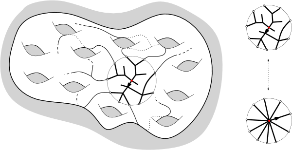
Figure 1: Illustration of the surgical operation

It is clear that this operation is invertible. To see that it is a bijection between the two sets in question we need to establish that it does not change the genus or number of faces in a map. One way to see this is based on an alternative description of the surgery, namely that it contracts every edge of $t$ except those incident to the leaves, and it is easy to see that edge contraction does not change the number of faces or genus of a map.

∎

3.2 Identifying the limit

Recall that for $\xi\in(0,1)$ we denote by $T_{\xi}$ the law of a Galton-Watson tree with $\operatorname{Geom}(\xi)-1$ offspring distribution. Note that when $\xi\in(0,1/2)$ the mean offspring is strictly greater than $1$ and so the process is supercritical, and recall that $T^{\infty}_{\xi}$ is $T_{\xi}$ conditioned to survive. Plane trees can be viewed as maps, rooted at the edge from the root to its first child. For every $r\geq 0$, if $t$ is a (possibly infinite) plane tree we denote by $B_{r}(t)$ the rooted subtree of $t$ made of all the vertices at height less than or equal to $r$.

Proposition 7.

Fix $\xi\in(0,1/2)$. For any tree $t$ of height exactly $r$ having $k$ edges and exactly $d$ vertices at maximal height, we have

$$\mathbb{P}\big{(}B_{r}(T^{\infty}_{\xi})=t\big{)}=\frac{\big{(}\xi(1-\xi)\big{)}^{k+1-d}\big{(}(1-\xi)^{d}-\xi^{d}\big{)}}{1-2\xi}.$$

Note that the probability of observing $t$ does not depend on $r$, but only on the number of edges and vertices where $t$ is connected to the rest of $T_{\xi}$.

Proof.

Since $\xi\in(0,1/2)$ the Galton-Watson process is supercritical and by standard result the extinction probability $p_{\mathrm{die}}$ is strictly less than $1$ and is the root of $x=\sum_{k\geq 0}x^{k}(1-\xi)^{k}\xi$ in $(0,1)$. Hence

$$p_{\mathrm{die}}=\frac{\xi}{1-\xi}.$$

Next, fix a tree $t$ of height exactly $r$ with $k$ edges and $d$ vertices at height $r$. By the definition of $T_{\xi}$ if $k_{u}$ denotes the number of children of the vertex $u$ in $t$ we have

$$\mathbb{P}(B_{r}(T_{\xi})=t)=\prod_{u}(1-\xi)^{k_{u}}\xi=(1-\xi)^{k}\xi^{k+1-d}$$

where the product is taken over all the vertices of $t$ which are at height less than $r$. Conditioned on the event $\{B_{r}(T_{\xi})=t\}$, by the branching property, the probability that the tree survives forever is $(1-p_{\mathrm{die}}^{d})$. Combining the pieces, we get the statement of the proposition. ∎

Proof of Theorem 1 for $\theta\in(0,1/2)$.

Under the assumptions of Theorem 1, fix $r$ and let $t$ be a rooted oriented tree of height exactly $r$ having $k$ edges and exactly $d$ vertices at height $r$. By Lemma 6 we have

$$\mathbb{P}(B_{r}(U_{n,g_{n}})=t) =\frac{\#\{m\in\mathcal{U}_{g_{n},n-k+d}\mbox{ with root degree }d\}}{\#\mathcal{U}_{g_{n},n}}$$

$$=\frac{\#\mathcal{U}_{g_{n},n-k+d}}{\#\mathcal{U}_{g_{n},n}}\cdot\mathbb{P}(\text{root degree of }U_{g_{n},n-k+d}=d).$$

Applying Theorem 4 we have

$$\mathbb{P}(\text{root degree of }U_{g_{n},n-k+d}=d)\xrightarrow[n\to\infty]{}\left(\frac{1-\beta_{\theta}^{2}}{4\beta_{\theta}}\right)\frac{(1+\beta_{\theta})^{d}-(1-\beta_{\theta})^{d}}{2^{d}}.$$ (3.1)

On the other hand, since $n/s=(n-k+d)/(s-k+d)+o(1/\sqrt{n})$ we can apply Theorem 3 for the asymptotic of $\#\mathcal{U}_{g_{n},n-k+d}$ and $\#\mathcal{U}_{g_{n},n}$ with the same sequence $(\beta_{n})$ and get that

$$\frac{\#\mathcal{U}_{g_{n},n-k+d}}{\#\mathcal{U}_{g_{n},n}}\sim\frac{(2n+2d-2k)!n!s!Z_{\beta_{n}}^{d-k}}{(2n)!(n+d-k)!(s+d-k)!\beta_{n}^{d-k}}.$$

Since $d,k$ are fixed, and using the facts that $\beta_{n}\to\beta_{\theta}$, $Z_{\beta_{n}}\to Z_{\beta_{\theta}}$ and $s/n\to(1-2\theta)$, the last display is also equivalent to

$$\frac{\#\mathcal{U}_{g_{n},n-k+d}}{\#\mathcal{U}_{g_{n},n}}\sim\left(\frac{\beta_{\theta}(1-2\theta)}{4Z_{\beta_{\theta}}}\right)^{k-d}=\left(\frac{1-\beta_{\theta}^{2}}{4}\right)^{k-d},$$ (3.2)

by the definition of $\beta_{\theta}$ in eq. 2.1. Plugging (3.1) and (3.2) together and using Proposition 7 we find that

$$\mathbb{P}(B_{r}(U_{g_{n},n})=t)\xrightarrow[n\to\infty]{}\mathbb{P}(B_{r}(T^{\infty}_{\xi_{\theta}})=t),$$

with $\xi_{\theta}=(1-\beta_{\theta})/2$.

Finally, note that the law of $B_{r}(T^{\infty}_{\xi_{\theta}})$ is a probability measure on the set of finite plane trees. It follows that $B_{r}(U_{g_{n},n})$ is tight, and converges in distribution to $B_{r}(T^{\infty}_{\xi_{\theta}})$. Since $r$ is arbitrary, this completes the proof of the Theorem. ∎

4 Questions and remarks

Planarity.

A consequence of Theorem 1 is that $U_{g_{n},n}$ is locally a tree (hence planar) near its root. More precisely, the length of a minimal non-trivial cycle containing the root edge diverges in probability as $n\to\infty$. A much stronger statement has been proved in [11] where quantitative estimates on cycle lengths are obtained. As noted above, our proof does not rely on this result and our approach is softer. Note that our method of proof only requires to prove convergences of the quantities $\mathbb{P}(B_{r}(U_{g_{n},n})=t)$ when $t$ is a tree since we were able to identify these limits as coming from a probability measure on infinite trees.

Open questions.

We gather here a couple of possible extensions of our work.

Question 1.

Find more precise asymptotic formulae for $\#\mathcal{U}_{g,n}$ as $g,n\to\infty$. Theorem 3 gives a first order approximation.

Question 2.

Quantitatify the convergence of $U_{g_{n},n}$ to $T_{\xi_{\theta}}$. In particular, let $r_{n}=o(\log n)$. Is it possible to couple $U_{g_{n},n}$ with $T_{\xi_{\theta}}$ so that $B_{r_{n}}(U_{g_{n},n})=B_{r_{n}}(T_{\xi_{\theta}})$ with high probability?

Omer Angel, Gourab Ray
Department of Mathematics, University of British Columbia, Canada
{angel,gourab}@math.ubc.ca

Guillaume Chapuy
CNRS and LIAFA Université Paris Diderot - Paris 7, France
guillaume.chapuy@liafa.univ-paris-diderot.fr

Nicolas Curien
CNRS and LPMA Université Pierre et Marie Curie - Paris 6, France
nicolas.curien@gmail.com

References

- [1] O. Angel and G. Ray, Classification of half planar maps, arXiv:1303.6582, (2013).
- [2] O. Angel and O. Schramm, Uniform infinite planar triangulations, Comm. Math. Phys., 241 (2003), pp. 191–213.
- [3] I. Benjamini, Random planar metrics, Proceedings of the ICM 2010, (2010).
- [4] I. Benjamini and O. Schramm, Recurrence of distributional limits of finite planar graphs, Electron. J. Probab., 6 (2001), pp. no. 23, 13 pp. (electronic).
- [5] J. Bettinelli, The topology of scaling limits of positive genus random quadrangulations, Ann. Probab., 40 (2012), pp. 1897–1944.
- [6] G. Chapuy, V. Féray, and É. Fusy, A simple model of trees for unicellular maps, J. Combin. Theory Ser. A, 120 (2013), pp. 2064–2092.
- [7] G. Chapuy, M. Marcus, and G. Schaeffer, A bijection for rooted maps on orientable surfaces, SIAM J. Discrete Math., 23 (2009), pp. 1587–1611.
- [8] B. Gosztonyi, Uniform infinite triangulations on the sphere and on the torus., MSc thesis ELTE TTK, (2012).
- [9] A. Goupil and G. Schaeffer, Factoring -cycles and counting maps of given genus, European J. Combin., 19 (1998), pp. 819–834.
- [10] V. V. Petrov, Sums of independent random variables, Springer-Verlag, New York, 1975. Translated from the Russian by A. A. Brown, Ergebnisse der Mathematik und ihrer Grenzgebiete, Band 82.
- [11] G. Ray, Large unicellular maps in high genus. arXiv:1307.1224.
- [12] T. R. S. Walsh and A. B. Lehman, Counting rooted maps by genus, J. Combin. Theory Ser. B., 13 (1972), pp. 192–218.