Emergent Newtonian dynamics and the geometric origin of mass

Abstract

We consider a set of macroscopic (classical) degrees of freedom coupled to an arbitrary many-particle Hamiltonian system, quantum or classical. These degrees of freedom can represent positions of objects in space, their angles, shape distortions, magnetization, currents and so on. Expanding their dynamics near the adiabatic limit we find the emergent Newton’s second law (force is equal to the mass times acceleration) with an extra dissipative term. In systems with broken time reversal symmetry there is an additional Coriolis type force proportional to the Berry curvature. We give the microscopic definition of the mass tensor relating it to the non-equal time correlation functions in equilibrium or alternatively expressing it through dressing by virtual excitations in the system. In the classical (high-temperature) limit the mass tensor is given by the product of the inverse temperature and the Fubini-Study metric tensor determining the natural distance between the eigenstates of the Hamiltonian. For free particles this result reduces to the conventional definition of mass. This finding shows that any mass, at least in the classical limit, emerges from the distortions of the Hilbert space highlighting deep connections between any motion (not necessarily in space) and geometry. We illustrate our findings with four simple examples.

1 Introduction

Newton’s second law, $F=m\ddot{X}$, applies to a wide range of phenomena and it is the cornerstone of the classical physics. This equation certainly describes the motion of particles in free space but it also predicts the dynamics of macroscopic objects like rotating bodies where $X$ represents the angle and $m$ is the moment of inertia or the behavior of the electrical current in a LC circuits where $X$ is a current and $m$ is a combination of capacitance and inductance.

However, as we all know, when an object moves through a medium it dissipates energy into the surrounding environment increasing its entropy and, as a result, it slows down and eventually stops. In this case, to properly describe the object’s dynamics, Newton’s law need to be supplemented with a dissipative (drag) term:

$$m\ddot{X}+\eta\dot{X}=F.$$ (1)

Drag is not specific to the motion in real space and it is present every time a physical quantity changes in time. For example, when the magnetic flux through a coil is increased in time, the environment (electrons in the coil) will react by producing a drag force which opposes this change (i.e. the Faraday’s law). Likewise coherent spin oscillations always decay in time due to dissipation in the spin environment and so on.

A pragmatic and very successful approach consists in seeing the mass $m$ and the dissipation $\eta$ in Eq. (1) as emergent properties (i.e. phenomenological parameters) which need to be fitted to reproduce the correct dynamics of macroscopic degrees of freedom. This approach is conceptually unsatisfactory and, for this reason, a lot of research effort has been focused on trying to derive the mass and the dissipation from a more fundamental theory (see e.g. Refs. [1, 2, 3, 4]). Normally one starts from the microscopic approach for both the object and the medium and using various approximations derives effective equations of motion for the macroscopic degree of freedom (d.o.f.) [5, 6, 7, 8, 9]. From this approach one finds both renormalization of the bare mass by dressing with elementary excitations and the drag force (see for example [10]). For example, in the Landau-Fermi Liquid theory [11, 12] the electron-electron interaction lead to a renormalization of the bare electron mass (and other dynamical properties).

In this work we take a different approach (see [2] and references therein), where we use statistical equilibrium of a complex system as a starting point. Namely we consider an arbitrary many-body system with possibly infinitely many degrees of freedom interacting with few macroscopic parameters $\vec{\lambda}(t)$, which are allowed to slowly change in time (see Fig.1). We assume that if $\vec{\lambda}$ is constant the system equilibrates at some temperature (as we will discuss later this assumption can be further relaxed). By extending the Kubo linear response theory [13] to such setups we provide a framework to compute the energy exchange between the many-body system and macroscopic d.o.f. in time derivatives of $\vec{\lambda}(t)$. In the first two orders (for systems with time-reversal invariance) the resulting expression takes the form of the Newton’s second law with the additional drag term:

$$\kappa_{\nu\mu}\ddot{\lambda}_{\mu}+\eta_{\nu\mu}\dot{\lambda}_{\mu}=M_{\nu},$$ (2)

where $\kappa_{\nu\mu}$ is the mass tensor, $\eta_{\nu\mu}$ is the drag tensor, and $M_{\nu}$ is the force (we choose this notation to reserve the letter $F$ for the Berry curvature). In the absence of symmetries all three coefficients can explicitly depend on $\vec{\lambda}$ predicting nontrivial dynamics. We express $\kappa$ and $\eta$ through the non-equal time equilibrium correlation functions and show that in general the mass is related to virtual (off-shell) excitations while the drag coefficient is determined by real (on-shell) processes. The expansion in derivatives of $\dot{\lambda}_{\mu}$ used to derive Eqs. (2) relies on the time scale separation between slow dynamics of the microscopic parameters $\vec{\lambda}$ and the fast dynamics of the system coupled to $\vec{\lambda}$. In the situations where this time scale separation does not hold, e.g. near phase transitions or low dimensional gapless system the validity of the expansion in time derivatives of $\vec{\lambda}$ should be checked on the case by case basis (see Sec. 3.2.2).

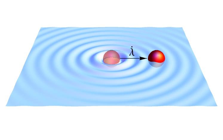
Figure 1: (Color on-line) Schematic setup considered. A macroscopic d.o.f. is initially at equilibrium (light red ball) with a complex environment (indicated by the wave-background). Then it starts moving with velocity $\dot{\lambda}$ through the environment, which has to rearrange, and generates both a drag force and a renormalization of the mass of the d.o.f.. The drag coefficient is related to real transitions between eigenstates of the environment (see Eq. (24)) while the mass is related to virtual transitions which describe dressing of the d.o.f. by the virtual exvitations of the environment (see Eq. (26)).

Our result for the drag coefficient in Eq. (2) agrees with the recent classical result of Ref. [14] and, as shown there, can be used to define the dissipative metric. In addition we find that in the high-temperature or classical limit the mass tensor $\kappa$ is equal to the product of the inverse temperature and the thermally averaged Fubini-Study metric tensor $g_{\mu\nu}$. The latter characterizes deformations of the eigenstates of the systems to the change of $\vec{\lambda}$ [15, 16, 17]:

$$\kappa_{\nu\mu}=\beta g_{\nu\mu}$$ (3)

This result allows one to interpret the (inertial) mass as an emergent property deriving from the response of the Hilbert space to the change of $\vec{\lambda}$. This statement echoes the result in general relativity in which the mass is seen as an emergent property which stems from the curvature of space-time. Let us point that the metric tensor $g_{\mu\nu}$ is equal to the covariance matrix of the gauge potentials $\mathcal{A}_{\mu}=i\partial_{\mu}$  responsible for the translations in the parameter space [17]: $2g_{\mu\nu}=\langle\mathcal{A}_{\mu}\mathcal{A}_{\nu}\rangle_{c}+\mu\leftrightarrow\nu\equiv\langle\mathcal{A}_{\nu}\mathcal{A}_{\mu}\rangle-\langle\mathcal{A}_{\nu}\rangle\langle\mathcal{A}_{\mu}\rangle+\mu\leftrightarrow\nu$, where $\langle\dots\rangle$ implies averaging with respect to the equilibrium density matrix. For translations in real space this gauge potential is nothing but the momentum operator $\mathcal{A}_{x}=p_{x}$, for rotations in $xy$ plain it is the angular momentum operator $\mathcal{A}_{\phi}=L_{z}$. In general these gauge potentials are complicated many-body operators, which however satisfy properties of locality [17]. For simple setups like a free particle in a vacuum our result $m=\kappa_{xx}=\beta\langle p_{x}^{2}\rangle$ reduces to a conventional equipartition theorem $\langle p_{x}^{2}\rangle=mT$ (see Sec 5.1 for a detailed example). So this finding shows that even ordinary mass of a particle has a direct geometric interpretation and is related to the distortion of the Hilbert space surrounding the particle as it moves in space. At arbitrary temperatures instead of Eq. (3) we obtain

$$2\kappa_{\nu\mu}=\int_{0}^{\beta}d\tau\,\,\langle\mathcal{A}_{H,\nu}(-i\tau)\mathcal{A}_{H,\mu}(0)+\nu\leftrightarrow\mu\rangle_{0,c},$$ (4)

where $\mathcal{A}_{H,\mu}(-i\tau)$ is the imaginary time Heisenberg representation of the gauge potential. In the high-temperature limit Eq. (4) obviously reduces to Eq. (3). This general expression can serve as the formal definition of the mass tensor for an arbitrary system. It also can be thought of as an extension of the equipartition theorem to quantum systems.

In less trivial situations of interacting systems and motion in the parameter space rather than the real space our results suggest an experimentally feasible way to indirectly measure the Fubini-Study metric and to directly analyze the quantum geometry of the system including various singularities and geometric invariants [17]. We illustrate how this can be done by analyzing three simple examples (Sec. 5).

2 Setup and main results

We consider the following Hamiltonian:

$$H_{tot}(\vec{\lambda})=H_{0}(\vec{\lambda})+H(\vec{\lambda}),$$ (5)

where $H_{0}(\vec{\lambda})$ is the Hamiltonian describing the bare motion of the macroscopic d.o.f. $\vec{\lambda}$, which can be multi-component and $H(\vec{\lambda})$ is the Hamiltonian of the interacting system of interest which depends on $\vec{\lambda}$. The choice of splitting $H_{tot}$ between $H_{0}$ and $H$ is somewhat arbitrary and we can well choose $H_{0}=0$ so that $H_{tot}=H$, however, for an intuitive interpretation of the results, it is convenient to assume that $H_{0}(\vec{\lambda})$ represents a massive degree of freedom in some external potential $V(\vec{\lambda})$:

$$H_{0}(\vec{\lambda})=\frac{\vec{p}_{\lambda}^{\,2}}{2m}+V(\vec{\lambda}).$$

In the infinite mass limit ($m\rightarrow\infty$), $\vec{\lambda}$ represents an external (control) parameter whose dynamics is specified a priori. When $m$ is finite, $\vec{\lambda}$ is a dynamical variable and its dynamics needs to be determined self-consistently.

One can identify two different sources of the energy change in the system. The first contribution is related to the dependence of the energy eigenstates of the system on $\vec{\lambda}$. This contribution does not vanish in the adiabatic limit and it is reversible. The second contribution is related to the excitations created in the system and, as we shall see, it contains both reversible and irreversible terms. To shorten the notation we term the first contribution as the adiabatic work and the second one as the heat.

Formally these two contributions can be defined as:

$$\partial_{t}\langle H\rangle(t)\equiv Tr\left\{\partial_{t}\left(H(t)\rho(t)\right)\right\}=\dot{W}(t)+\dot{Q}(t)$$

where $\rho(t)$ is the density matrix and the adiabatic work rate, $\dot{W}(t)$, and the heat rate, $\dot{Q}(t)$, are defined as:

$$\dot{W}(t)=\dot{\vec{\lambda}}\sum_{n}\frac{\partial\epsilon_{n}}{\partial\vec{\lambda}}\,\rho_{n}(t)=\dot{\vec{\lambda}}\cdot\nabla_{\vec{\lambda}}E(\vec{\lambda})\equiv-\dot{\vec{\lambda}}\,\cdot M_{\vec{\lambda}},$$ (6)

$$\dot{Q}(t)=\sum_{n}\dot{\rho}_{n}(t)\,\epsilon_{n},$$ (7)

where $E=\sum_{n}\epsilon_{n}\rho_{n}$ is the total energy of the system, $\rho_{n}(t)$ is the probability of occupying the $n$-th instantaneous energy eigenstate, $\epsilon_{n}$ is the instantaneous energy and $M_{\vec{\lambda}}=-\nabla_{\vec{\lambda}}E(\vec{\lambda})$ is the conventional generalized force which we introduced in Eq. (2) [18]. This force appears, for example, in the Born-Oppenheimer approximation schemes in which the energy of the electrons, calculated for fixed ions’ positions, acts as a potential for the (classical) motion of the ions.

In the strictly adiabatic limit, according to the quantum adiabatic theorem, there are no transitions between the instantaneous energy levels and $\dot{Q}=0$.  Using time-dependent perturbation theory to second order in $\dot{\lambda}$, we have computed $\dot{\rho}(t)$, and obtained the leading non-adiabatic contributions to the heat production rate (see Appendix A):

$$\begin{split}\dot{Q}(t)&=\dot{\lambda}_{\nu}(t)\int_{0}^{t}dt^{\prime}\int_{0}^{\beta}d\tau\,\dot{\lambda}_{\mu}(t-t^{\prime})\langle\mathcal{M}_{H,\nu}(t)\mathcal{M}_{H,\mu}(t-t^{\prime}+i\tau)\rangle_{0,c}\\ &=\dot{\lambda}_{\nu}(t)\int_{0}^{t}dt^{\prime}\,\dot{\lambda}_{\mu}(t-t^{\prime})\sum_{n\neq m}\frac{\rho^{0}_{n}-\rho^{0}_{m}}{\epsilon_{m}-\epsilon_{n}}e^{i(\epsilon_{m}-\epsilon_{n})t^{\prime}}\langle m_{\lambda}|\mathcal{M}_{\nu}|n_{\lambda}\rangle\langle n_{\lambda}|\mathcal{M}_{\mu}|m_{\lambda}\rangle\end{split}$$ (8)

where we imply summation over repeated indices, $|n_{\lambda}\rangle$ denote the (many-body) eigenstates of the Hamiltonian $H(\vec{\lambda}(t))$ with energies $\epsilon_{n}$, $\rho^{0}_{n}$ is the initial stationary occupation probability which, for the most of the paper, we assume to be thermal $\rho_{n}=\exp[-\beta\epsilon_{n}]/Z$, $c$ implies the connected part of the correlation function and

$$\mathcal{M}_{H,\nu}(t)=-\exp[iHt]\left(\partial_{\lambda_{\nu}}H\right)\exp[-iHt]$$ (9)

is the Heisenberg representation (for time-independent Hamiltonian) of the conjugate force coupled to $\lambda_{\nu}$. The equilibrium expectation value of this force $\langle\mathcal{M}_{\lambda}\rangle_{0}=M_{\lambda}=-\nabla_{\vec{\lambda}}E(\vec{\lambda})$ is the conventional generalized force introduced earlier. Note that $\epsilon_{n}$ and $|n\rangle$ are the many-body levels and many-body eigenstates of the full interacting system (including the bath if it is present). If the system is weakly coupled to the bath then Eq. (8) can be simplified using standard tools of the many-body perturbation theory [19]. For simplicity in Eq. (8) and (9) we assume that the energy spectrum $\epsilon_{n}$ does not change with $\vec{\lambda}$ but in the Appendix A we show a complete derivation without such an assumption. Then essentially by energies $\epsilon_{n}$ and the matrix elements one needs to understand instantaneous values taken at time $t$ (see Appendix A). Eq. (8) applies to arbitrary times $t$ and as such describes both transient and the long time regimes. It is clear that if $t$ becomes longer than the relaxation time then the heat production rate becomes insensitive to the initial time $t=0$ but, for small isolated systems and at low temperatures, transients can be important (see Sec. 5.3 for an example). This expression generalizes an earlier result by D. A. Sivak and G. E. Crooks [14] to quantum systems at arbitrary temperatures. In the high temperature (or classical) limit the integration over the imaginary time component $\tau$ reduces to a factor of the inverse temperature $\beta$ and we recover Eq. (11) from Ref. [14].

If the rate $\dot{\vec{\lambda}}$ changes slowly in time on the scales determined by the relaxation rate in the system then we can expand Eq. (8) to the leading order in time derivatives of $\vec{\lambda}$. For systems with the Hamiltonian $H$ obeying time-reversal symmetry we get (terms proportional to higher time derivatives of $\vec{\lambda}$ are discussed in Appendix B)

$$\dot{Q}(t)=\dot{\lambda}_{\nu}\eta_{\nu\mu}\dot{\lambda}_{\mu}+\dot{\lambda}_{\nu}\kappa_{\nu\mu}\ddot{\lambda}_{\mu}$$ (10)

The first term represents the usual drag or friction tensor and the second term (as we will see below) amounts to the mass renormalization of the external parameter. At zero temperature the first dissipative term generically vanishes as required by the fluctuation-dissipation relations while the second contribution remains finite. Both tensors $\eta$ and $\kappa$ are symmetric under $\nu\leftrightarrow\mu$ and positive semi-definite (assuming positive temperature). Before describing the friction and mass tensors in details we discuss some consequences of our main result (10).

3 Implications of Eq.(10).

3.1 Energy absorption in a driven system

As the first implication of our results, we discuss qualitative features of energy absorption in systems driven by the external parameter $\vec{\lambda}(t)$. We will be interested in protocols longer than the relaxation time in the system such that susceptibilities $\eta$ and $\kappa$ become effectively time independent (at shorter times one expects transients, which can be analyzed using the short time expansion of Eq. (8)). To avoid possible singularities we assume that the protocol starts smoothly in time, i.e. $\dot{\vec{\lambda}}(0)=0$. Integrating Eq. (10) we find

$$Q(t)\approx\eta_{\mu\nu}\int_{0}^{t}dt^{\prime}\dot{\lambda_{\mu}}(t^{\prime})\dot{\lambda}_{\nu}(t^{\prime})+\frac{\kappa_{\mu\nu}}{2}\dot{\lambda}_{\mu}(t)\dot{\lambda}_{\nu}(t)+\dots$$ (11)

From this expression we see that indeed $\eta$ plays the role of dissipation while $\kappa$ plays the role of the additional mass associated with the dressing of the parameter $\lambda$ by excitations. It is clear that the first (dissipative) term gives a contribution proportional to the total duration of the process and it is dominant at long times $t\to\infty$. However, at low temperatures or nearly isolated small systems the coefficient $\eta$ can be very small and the second (mass) term can be dominant for long times. In particular, if $\dot{\lambda}(t)$ approaches a constant value, after an initial transient, $Q(t)$ will display a plateau for $t\lesssim t^{\ast}=\kappa/\eta$.

3.2 Emergent equations of motion

Next we consider $\vec{\lambda}$ to be a dynamic d.o.f. describing a “particle” coupled to a many-body system and study its dynamics.

3.2.1 Dynamics of a scalar particle.

First let us assume that $\vec{\lambda}$ is a single component scalar object. The Hamiltonian is given by Eq. (5). Noting that the total energy of the particle and the system is conserved and using Eq. (6) and Eq. (10) we find

$$\begin{split}&\frac{d}{dt}\left[\frac{m\dot{\lambda}^{2}}{2}+V(\lambda)+E(\lambda)\right]=0\,\Rightarrow\,m\dot{\lambda}\ddot{\lambda}+\dot{\lambda}\partial_{\lambda}V+\dot{W}+\dot{Q}=0,\\ &\Rightarrow\,m\dot{\lambda}\ddot{\lambda}+\dot{\lambda}\partial_{\lambda}V-\dot{\lambda}M_{\lambda}+\eta\dot{\lambda}^{2}+\kappa\dot{\lambda}\ddot{\lambda}=0.\end{split}$$ (12)

Dividing this equation by $\dot{\lambda}$ we find

$$(m+\kappa)\ddot{\lambda}+\dot{\lambda}\eta=-\frac{\partial V}{\partial\lambda}+M_{\lambda}$$ (13)

i.e. we find that near the slow limit the dynamics of $\lambda$ is given by the classical Newton’s equations of motion with an additional dissipative term. Note that the Newtonian form of the equation of motion (13) was not postulated. It rather emerges from the leading non-adiabatic expansion of the density matrix describing the system coupled to $\vec{\lambda}$. Thus the effect of the system on the dynamics of the macroscopic d.o.f. reduces to three contributions: mass renormalization ($\kappa$), drag coefficient ($\eta$), and an extra force ($M_{\lambda}$). As mentioned earlier, $M_{\lambda}$ is the force which appears in the Born-Oppenheimer approximation in which the only effect of the system is to lead to an effective (conservative) potential for the motion of the macroscopic d.o.f.. For example in this approximation schemes the electrons in a solid lead to an effective potential for the motion of the ions. By considering the non-adiabatic correction to the energy of the system, which we named heat (see Eq. (8)), we go beyond the Born-Oppenheimer approximation and find the emergent Newton’s equation (13). Note that in general $\kappa$, $\eta$ and $M_{\lambda}$ depend on $\lambda$ and Eq. (13) can predict non-trivial dynamics. As we pointed earlier the Hamiltonian $H_{0}$ can be absorbed into the definition of $H$. In this case $m=0$ and $\partial_{\lambda}V=0$ and Eq. (13) reduces to the scalar version of Eq. (2). Moreover when $H_{0}=0$ the total mass and the total force are entirely determined by the interactions with the system. Let us note that when $\kappa$ depends on $\vec{\lambda}$ it is more accurate to write the mass term in Eq. (13) as $\frac{d}{dt}(\kappa\dot{\lambda})$. The difference between this term and $\kappa\ddot{\lambda}$ is of order $\dot{\lambda}^{2}$ and it is beyond the accuracy of our expansion. However a more careful analysis shows that this term is energy conserving, which implies that it comes from the full derivative of $\kappa\dot{\lambda}^{2}$.

3.2.2 Berry curvature and Coriolis force.

The previous derivation of the equations of motion was based on using the conservation of the total energy conservation leading to Eq. (12) and dividing it by $\dot{\lambda}$. For a multicomponent parameter energy conservation is not sufficient to fix the equations of motion, since, as it is well known in the case of rotations or magnetic field, the Coriolis or the Lorentz forces affect the dynamics but not the energy. To proceed within the same framework of non-adiabatic response we can evaluate the expectation value of the generalized force $\langle\mathcal{M}_{\nu}\rangle(t)\equiv Tr\left[\rho(t)\mathcal{M}_{\nu}\right]$. We give the details of the derivation in Appendix A and here only quote the final result obtained using the same approximation as Eq. (8):

$$\langle\mathcal{M}_{\nu}\rangle(t)=M_{\nu}-\int_{0}^{t}dt^{\prime}\dot{\lambda}_{\mu}(t-t^{\prime})\,\sum_{n\neq m}\frac{\rho_{n}^{0}-\rho_{m}^{0}}{\epsilon_{m}-\epsilon_{n}}\mathrm{e}^{i(\epsilon_{m}-\epsilon_{n})t^{\prime}}\langle m_{\lambda}|\mathcal{M}_{\nu}|n_{\lambda}\rangle\langle n_{\lambda}|\mathcal{M}_{\mu}|m_{\lambda}\rangle.$$ (14)

We remind that the generalized force $M_{\nu}$ is by definition the equilibrium expectation value of $\mathcal{M}_{\nu}$. If we now do the expansion of $\dot{\lambda}_{\mu}(t-t^{\prime})$ near $t^{\prime}=0$ up to the second derivative we find [20]

$$\langle\mathcal{M}_{\nu}(t)\rangle=M_{\nu}+F_{\nu\mu}\dot{\lambda}_{\mu}-\eta_{\nu\mu}\dot{\lambda}_{\mu}-\kappa_{\nu\mu}\ddot{\lambda}_{\mu}-F^{\prime}_{\nu\mu}\ddot{\lambda}_{\mu},$$ (15)

where

$$F_{\nu\mu}=i\langle[\mathcal{A}_{\nu},\mathcal{A}_{\mu}]\rangle=i\sum_{n}\rho^{0}_{n}\langle n_{\lambda}|\overleftarrow{\partial}_{\nu}\overrightarrow{\partial}_{\mu}-\overleftarrow{\partial}_{\mu}\overrightarrow{\partial}_{\nu}|n_{\lambda}\rangle$$ (16)

is the Berry curvature and

$$F^{\prime}_{\mu\nu}=i\pi\sum_{n\neq m}\,\frac{\rho_{n}^{0}-\rho_{m}^{0}}{\epsilon_{n}-\epsilon_{m}}\langle m_{\lambda}|\mathcal{M}_{\nu}|n_{\lambda}\rangle\langle n_{\lambda}|\mathcal{M}_{\mu}|m_{\lambda}\rangle\,\delta^{\prime}(\epsilon_{n}-\epsilon_{m})$$ (17)

is another on-shell antisymmetric tensor ($\delta^{\prime}(x)$ stands for the derivative of the delta-function) and $\eta$ and $\kappa$ are the friction and the mass tensors discussed before. Without the acceleration terms Eq. (15) extends earlier results on the dynamical Hall response [21, 22, 23] to finite temperatures and possibly open systems without extra assumptions about the Lindbladian dynamics [4]. As in the familiar situation of the current response to the electric field (time dependent vector potential) the transverse Hall like response determined by the Berry curvature is non-dissipative (off-shell) while the longitudinal on-shell response proportional to the drag $\eta$ is directly related to dissipation [19].

We can now self-consistently combine Eq. (15) with the classical (Lagrangian) equations of motion for the parameter $\vec{\lambda}$:

$$m_{\nu\mu}\frac{d\lambda_{\nu}}{dt}=p_{\nu},\quad\frac{dp_{\nu}}{dt}=-\frac{\partial V}{\partial\lambda_{\nu}}+\langle\mathcal{M}_{\nu}(t)\rangle$$ (18)

and get the multicomponent dissipative Newton’s equations:

$$(m_{\nu\mu}+\kappa_{\nu\mu}+F^{\prime}_{\nu\mu})\ddot{\lambda}_{\mu}+(\eta_{\nu\mu}-F_{\nu\mu})\dot{\lambda}_{\mu}=-\frac{\partial V}{\partial\lambda_{\nu}}+M_{\nu}.$$ (19)

which generalize Eq. (13). The first term in this equation represents the renormalized mass (as we discussed we can choose the bare mass to be zero by absorbing $H_{0}$ into $H$). The term $\eta_{\nu\mu}\dot{\lambda}_{\mu}$ is the dissipative term also appearing in the single component case. And finally there are two new antisymmetric terms, one proportional to the Berry curvature is clearly the analogous of the Coriolis force and the other antisymmetric on-shell contribution encoded in $F^{\prime}$ is effectively antisymmetric mass term. This suggests that the Berry curvature can be indirectly measured via the Coriolis force acting upon a macroscopic d.o.f. [24]. In systems with time-reversal symmetry the two tensors $F,F^{\prime}$ vanish [25] and therefore, by fitting the long time dynamics of $\vec{\lambda}(t)$ to Eq. (19) with the additional knowledge of equilibrium generalized force one can extract both the drag tensor, $\eta_{\nu\mu}$, and the mass tensor, $\kappa_{\nu\mu}$. We emphasize again that, at high temperatures, the mass tensor reduces to the Fubini-Study metric tensor which is a covariance matrix of the gauge potential, or the momentum operator, which translates the Hamiltonian eigenstates in the parameter space. Therefore the very notion of the mass is related to the distance between eigenstates of the Hamiltonian $H(\vec{\lambda})$ induced by the change of the parameter $\vec{\lambda}$. Let us point that Eq. (26) [see below] essentially guarantees UV convergence of the mass as long as the variance of the generalized force is finite. On the contrary in gapless systems or near singularities like continuous phase transitions or glassy systems where correlation functions slowly decay in time the mass can acquire infra-red divergences and the energy absorption becomes non-analytic function of the rate as discussed in Ref. [26].

Equation (19) has another interesting implication. At zero temperature both dissipative tensors ($\eta$ and $F^{\prime}$) vanish (unless the system is tuned to a critical point or if it has gapless low-dimensional excitations [26]). In this case Eq. (19) can be viewed as a Lagrangian equations of motion. If fact, it is easy to see that the Lagrangian:

$$\mathcal{L}=\frac{1}{2}\,\dot{\lambda}_{\nu}\,(m+\kappa)_{\nu\mu}\,\dot{\lambda}_{\mu}+\dot{\lambda}_{\mu}\,A_{\mu}(\vec{\lambda})-V(\vec{\lambda})-E_{0}(\vec{\lambda})$$ (20)

reproduces Eq. (19) where $A_{\mu}(\vec{\lambda})=\langle 0_{\lambda}|\mathcal{A}_{\mu}|0_{\lambda}\rangle$ and $E_{0}(\vec{\lambda})=\langle 0_{\lambda}|H(\vec{\lambda})|0_{\lambda}\rangle$ are the value of the Berry connection and Hamiltonian (see (5)) in the instantaneous ($\vec{\lambda}$-dependent) ground state and we have used (see Eq. (16)):

$$\frac{\partial A_{\mu}}{\partial\lambda_{\nu}}-\frac{\partial A_{\nu}}{\partial\lambda_{\mu}}=i\left[\partial_{\nu}\langle 0_{\lambda}|\partial_{\mu}0_{\lambda}\rangle-\partial_{\mu}\langle 0_{\lambda}|\partial_{\nu}0_{\lambda}\rangle\right]=i\langle 0_{\lambda}|\overleftarrow{\partial}_{\nu}\overrightarrow{\partial}_{\mu}-\overleftarrow{\partial}_{\mu}\overrightarrow{\partial}_{\nu}|0_{\lambda}\rangle=F_{\nu\mu}.$$

From the Lagrangian (20) we can define the canonical momenta conjugate to the coordinates $\lambda_{\nu}$:

$$p_{\nu}\equiv\frac{\partial\mathcal{L}}{\partial\dot{\lambda}_{\nu}}=(m_{\nu\mu}+\kappa_{\nu\mu})\dot{\lambda}_{\mu}+A_{\nu}(\vec{\lambda})$$ (21)

and the emergent Hamiltonian:

$$\mathcal{H}\equiv\dot{\lambda}_{\nu}\,p_{\nu}-\mathcal{L}=\frac{1}{2}(p_{\nu}-A_{\nu})(m+\kappa)_{\nu\mu}^{-1}(p_{\mu}-A_{\mu})+V(\vec{\lambda})+E_{0}(\vec{\lambda}).$$ (22)

Clearly the Berry connection term plays the role of the vector potential. Thus we see that the whole formalism of the Hamiltonian dynamics for arbitrary macroscopic degrees of freedom is actually emergent. Without mass renormalization this Hamiltonian was first derived in Ref. [27] in which it was also shown that when the slow d.o.f. is quantum, there is an addittional force proportional to the Fubini-Study metric tensor $g_{\nu\mu}$. Away from the ground state the dissipative tensors ($\eta$ and $F^{\prime}$) are, in general, non-zero and it is not possible to reformulate Eq. (19) via Hamiltonian dynamics.

3.2.3 Dynamics of a conserved degree of freedom. Emergent equilibrium from dynamics.

It is straightforward to apply the results above to the setup where two systems are coupled by a single conserved degree of freedom, i.e. $H=H_{1}(\lambda_{1})+H_{2}(\lambda_{2})$ with the additional constraint $\lambda_{1}+\lambda_{2}={\rm const}$. Then using the additivity of the mass $\kappa$ and drag $\eta$, which are obvious from the microscopic expressions (see Eq. (24) and (26) below) and invariance of Eq. (10) under $\lambda\to-\lambda$, we obtain the dissipative non-Markovian dynamics for $\lambda_{1}(t)$:

$$(\kappa_{1}+\kappa_{2})\ddot{\lambda}_{1}+(\eta_{1}+\eta_{2})\dot{\lambda}_{1}=M^{(1)}_{\lambda_{1}}-M^{(2)}_{\lambda_{2}}$$ (23)

We note that the Markovian limit of Eq. (23) is obtained by setting $\kappa_{1}=\kappa_{2}=0$. As expected from basic thermodynamics, the equilibrium between two systems ($\lambda_{1}=\text{const}$) is only possible when the generalized forces between two systems are equal to each other. Unlike in statistical mechanics, where this statement follows from the maximum entropy principle, here we explicitly derive this condition from the dynamical equilibrium. Note that this condition for the dynamical equilibrium does not require the two systems to be ergodic. In our derivation we only relied on starting from a stationary state, thermal or not.

4 Detailed description of friction and mass tensor

We now discuss the friction and mass tensors in details. The friction tensor can be expressed as [28]

$$\begin{split}\eta_{\nu\mu}&=\frac{1}{2}\int_{0}^{t}\,dt^{\prime}\int_{0}^{\beta}\,d\tau\langle\mathcal{M}_{H,\nu}(t^{\prime}-i\tau)\mathcal{M}_{H,\mu}(0)+\nu\leftrightarrow\mu\rangle_{c}\\ &=\sum_{n\neq m}\,\,\frac{\rho^{0}_{n}-\rho^{0}_{m}}{\epsilon_{m}-\epsilon_{n}}\,\langle m_{\lambda}|\mathcal{M}_{\nu}|n_{\lambda}\rangle\langle n_{\lambda}|\mathcal{M}_{\mu}|m_{\lambda}\rangle\,\frac{\sin\left((\epsilon_{m}-\epsilon_{n})t\right)}{\epsilon_{m}-\epsilon_{n}}\end{split}$$ (24)

from which it is clear that at positive temperatures (or more generally for any passive density matrix such that $(\rho^{0}_{n}-\rho^{0}_{m})(\epsilon_{m}-\epsilon_{n})>0$) the friction tensor is positive semi-definite and can therefore be used to define a metric. In particular, the metric associated with the friction $\eta$ was used in Ref. [29] for finding the paths of minimal dissipation in the parameter space. At long times, $t\rightarrow\infty$, we have

$$\frac{\sin(\epsilon_{m}-\epsilon_{n})t}{\epsilon_{m}-\epsilon_{n}}\to\pi\delta(\epsilon_{n}-\epsilon_{m}),\;\frac{\rho^{0}_{n}-\rho^{0}_{m}}{\epsilon_{m}-\epsilon_{n}}\,\to\beta\,\rho^{0}_{m}.$$

Therefore the friction tensor is defined by the on-shell processes, which is expected since we are dealing with slow, zero frequency, driving

$$\eta_{\nu\mu}=\pi\beta\sum_{n\neq m}\,\,\rho^{0}_{m}\langle m_{\lambda}|\mathcal{M}_{\nu}|n_{\lambda}\rangle\langle n_{\lambda}|\mathcal{M}_{\mu}|m_{\lambda}\rangle\delta(\epsilon_{n}-\epsilon_{m}).$$

So at $t\to\infty$ the drag is always determined by the high temperature asymptote of Eq. (8) (and thus the result of Ref. [14] always holds). At finite times, the expression for $\eta$ has different high temperature and low temperature asymptotes.

Similarly we can analyze the mass tensor $\kappa$

$$\kappa_{\nu\mu}=-\frac{1}{2}\int_{0}^{t}\,dt^{\prime}\,t^{\prime}\int_{0}^{\beta}\,d\tau\langle\mathcal{M}_{H,\nu}(t^{\prime}-i\tau)\mathcal{M}_{H,\mu}(0)+\nu\leftrightarrow\mu\rangle_{c},$$ (25)

which in the long time limit can be written as

$$\begin{split}\kappa_{\nu\mu}&=\sum_{n\neq m}\frac{\rho^{0}_{n}-\rho^{0}_{m}}{\left(\epsilon_{m}-\epsilon_{n}\right)^{3}}\,\langle m_{\lambda}|\mathcal{M}_{\nu}|n_{\lambda}\rangle\langle n_{\lambda}|\mathcal{M}_{\mu}|m_{\lambda}\rangle\\ &=\sum_{n\neq m}\frac{\rho^{0}_{n}-\rho^{0}_{m}}{\epsilon_{m}-\epsilon_{n}}\,\langle m_{\lambda}|\overleftarrow{\partial_{\lambda_{\nu}}}|n_{\lambda}\rangle\langle n_{\lambda}|\overrightarrow{\partial_{\lambda_{\mu}}}|m_{\lambda}\rangle\end{split}$$ (26)

where we have used the identity (see e.g. Ref. [30])

$$\left(\epsilon_{m}-\epsilon_{n}\right)\langle n_{\lambda}|\overrightarrow{\partial_{\lambda_{\mu}}}|m_{\lambda}\rangle=\langle n_{\lambda}|\mathcal{M}_{\mu}|m_{\lambda}\rangle$$

We emphasize again that we put aside the issue of convergence of the sum in Eq. (26) when we deal with macroscopic ergodic systems at finite temperatures. This convergence is essentially guaranteed if the non-equal time correlation functions entering Eq. (25) decay fast in time, which was our key assumption. Unlike for the friction tensor $\eta$, the mass tensor $\kappa_{\nu\mu}$ has, in the infinite time limit, non-vanishing asymptotes both in the high and zero-temperature limits. At low temperatures, $\beta\to\infty$,

$$\kappa_{\nu\mu}\approx\sum_{m\neq 0}\frac{\langle 0_{\lambda}|\mathcal{M}_{\nu}|m_{\lambda}\rangle\langle m_{\lambda}|\mathcal{M}_{\mu}|0_{\lambda}\rangle+\nu\leftrightarrow\mu}{\left(\epsilon_{m}-\epsilon_{0}\right)^{3}}.$$ (27)

At high temperatures (or near the classical limit) we find

$$\kappa_{\nu\mu}\approx\frac{\beta}{2}\sum_{m}\rho_{m}\,\left(\langle m_{\lambda}|\overleftarrow{\partial_{\lambda_{\nu}}}\,\overrightarrow{\partial_{\lambda_{\mu}}}|m_{\lambda}\rangle_{c}+\nu\leftrightarrow\mu\right)=\beta\,g_{\nu\mu}$$ (28)

where $g_{\nu\mu}$ is the finite temperature version Fubini-Study metric tensor characterizing statistical average of the distance between many-body eigenstates [17]. Let us mention that in traditional units the expressions for the mass Eqs. (26) - (28) should be multiplied by $\hbar^{2}$, which follows from the correct definition of the Gauge potentials $i\partial_{\lambda_{\mu}}\to i\hbar\partial_{\lambda_{\mu}}$. We also point that the mass tensor $\kappa$ can be written through the integrated connected imaginary time correlation function of the gauge potentials $\mathcal{A}_{\nu}$ and $\mathcal{A}_{\mu}$:

$$\kappa_{\nu\mu}=\frac{1}{2}\int_{0}^{\beta}d\tau\langle\mathcal{A}_{H,\nu}(-i\tau)\mathcal{A}_{H,\mu}(0)+\nu\leftrightarrow\mu\rangle_{0,c}$$ (29)

At high temperatures the imaginary time integral reduces to a factor $\beta$ and this result clearly reduces to Eq. (28). We point that the expressions for $\eta$ in the second line of (24) and for $\kappa$ in (26) apply to arbitrary stationary distributions $\{\rho^{0}_{n}\}$, not necessarily thermal.

It is interesting to note that short time transient dynamics also bears the geometric information. Thus integrating Eq. (8) over short times (and again assuming high temperature or classical limit) gives

$$Q(t)\approx\frac{\beta}{2}\,\delta\lambda_{\nu}(t)\,{f}_{\nu\mu}\,\delta\lambda_{\mu}(t),$$

where $\delta\lambda_{\nu}(t)\equiv\lambda_{\nu}(t)-\lambda_{\nu}(0)$ and

$$f_{\nu\mu}=\frac{1}{2}\langle\mathcal{M}_{\nu}\mathcal{M}_{\mu}+\mathcal{M}_{\mu}\mathcal{M}_{\nu}\rangle_{0,c}=\frac{\partial^{2}\ln(Z)}{\partial\lambda_{\mu}\partial\lambda_{\nu}}$$ (30)

is the thermodynamic metric tensor defined through the second derivative matrix of the partition function [32, 31].

5 Examples

5.1 Mass Renormalization of a particle interacting with identical quantum oscillators.

We now show explicitly how the mass of a classical object coupled to a quantum environment is renormalized. Let us consider the Hamiltonian (5) where

$$H_{0}=\frac{P_{\lambda}^{2}}{2\mu}+V(\lambda),\,\,\,H(\lambda)=\sum_{j=1}^{N}\left(\frac{\hat{p}_{j}^{2}}{2m}+\frac{k}{2}(\hat{x}_{j}-\lambda)^{2}\right)+\sum_{i>j}U(\hat{x}_{i}-\hat{x}_{j})$$

describes a macroscopic d.o.f. interacting with a collection of coupled quantum oscillators (QOs). We note that the coupling between the oscillators, $U(\hat{x}_{i}-\hat{x}_{j})$, does not need to be harmonic so instead of oscillators we can deal with interacting particles. Here, for simplicity we consider the $1$-dimensional case and $\hat{x}_{j}$ and $\hat{p}_{j}$ are quantum operators satisfying the usual commutation relations $\left[\hat{x}_{j},\hat{p}_{l}\right]=i\delta_{j,l}$ and we assume that the macroscopic d.o.f is subject to a constant external force, i.e. $-\partial_{\lambda}V(\lambda)=F_{0}$.

The basic expectation is that, due to the interaction between the macroscopic d.o.f. and the QOs, the macroscopic d.o.f. will drag the QOs with itself as it moves and as a consequence its mass will be renormalized. This expectation can be confirmed by analyzing the evolution of the center of mass of the system which, by definition, is determined only by the external forces $m_{eff}\ddot{X}_{cm}(t)=F_{0}$, where $m_{eff}=\mu+Nm$ is the total mass. The position of the macroscopic d.o.f. is the vector sum of the position of the center of mass and the relative coordinate (which will in general have an oscillatory behavior) $\lambda(t)=X_{cm}(t)+X_{\lambda}(t)$. We therefore conclude that, up to the oscillations of the relative coordinate, the macroscopic d.o.f. evolves with the renormalized mass $m_{eff}=\mu+Nm$ which can be several times larger than its bare mass $\mu$. If the coupling between oscillators is zero, $U=0$, the dynamics of the macroscopic d.o.f. can be solved exactly and it can be verified that our argument is correct and that the oscillations of the relative coordinate have frequency $\Omega\sim N^{1/2}$ and amplitude $B\sim N^{-1/2}$, which can be neglected for $N\gg 1$.

We now show how this behavior is reproduced using the emergent Newton’s law Eq. (13). Let’s first analyze the case of $N$ independent Harmonic Oscillators (HO), i.e. $U=0$. Then the drag term $\eta$ is zero since the harmonic oscillators have a discrete spectrum and there are not gapless excitations [33]. Moreover the extra force term $M_{\lambda}\equiv\sum_{n}\rho_{n}\partial_{\lambda}\epsilon_{n}$ is also zero since $\epsilon_{n}=\omega(n+\frac{1}{2})$ is independent on $\lambda$. Therefore we only need the mass tensor $\kappa$ which can be computed via Eq. (26) where $\mathcal{M}_{\lambda}\equiv-\partial_{\lambda}H=k(\hat{x}-\lambda)$. Expressing the position via the ladder operators $\hat{x}=\sqrt{\frac{1}{2m\omega}}(a+a^{\dagger})$ and using the standard properties $a|n\rangle=\sqrt{n}|n-1\rangle$ and $a^{\dagger}|n\rangle=\sqrt{n+1}|n+1\rangle$ together with the thermal occupations $\rho_{n}=e^{-\beta\omega n}\left(1-e^{-\beta\omega}\right)$ it is straightforward to show that $\kappa=m$. Since there are $N$ independent HOs each contributing equally to the renormalization of the mass Eq. (13) becomes:

$$(\mu+Nm)\ddot{\lambda}=F_{0}$$ (31)

in perfect agreement with our discussion above.

We can extend the above analysis to arbitrary interaction by using the equipartition theorem (see Eq. (26)): $\kappa=\beta\langle(\sum_{j}p_{j})(\sum_{l}p_{l})\rangle_{0}=\beta\langle p_{tot}^{2}\rangle_{0}=Nm$ where $p_{tot}=\sum_{j}p_{j}$ is the total momentum of the oscillators. Therefore even when $U\neq 0$ we find that the renormalized mass is $m_{eff}=\mu+Nm$.

5.2 Mass renormalization in a quantum piston.

Let us consider a massless spring connected to the potential wall. In this section we will explicitly insert all factors of $\hbar$. We also imagine that a quantum particle of mass $m$ is initially prepared in the ground state of the confining potential (see panel “a” in Fig. 2). As in the previous example we will compute how the mass of a classical object (the spring) coupled to a quantum environment (the potential well) is renormalized.

According to Eq. (27) the mass renormalization is given by

$$\kappa_{R}=2\hbar^{2}\sum_{n\neq 0}\frac{|\langle n_{\lambda}|\mathcal{M}|0_{\lambda}\rangle|^{2}}{(\epsilon_{n}-\epsilon_{0})^{3}},$$ (32)

where $\lambda=X_{R}$ is the position of the right potential wall. We approximate the confining potentail as a very deep square well potential. Then $\mathcal{M}\equiv-\partial_{\lambda}H=-V\delta(x-X_{R})$ and we find

$$\kappa_{R}=2\hbar^{2}\sum_{n\neq 0}\frac{V^{2}|\psi_{0}(X_{R})|^{2}|\psi_{n}(X_{R})|^{2}}{(\epsilon_{n}-\epsilon_{0})^{3}}.$$ (33)

Using the well known result for a finite (and deep) square well potentail

$$|\psi_{n}(X_{R})|=\sqrt{\frac{2}{L}}\,\,\sqrt{\frac{\epsilon_{n}}{V}}$$

where the factor of $\sqrt{2/L}$ comes from the normalizazion of the wave-function in a square potential of lenght $L$, we obtain

$$\kappa_{R}=2\hbar^{2}\left(\frac{2}{L}\right)^{2}\sum_{n\neq 0}\frac{\epsilon_{0}\epsilon_{n}}{(\epsilon_{n}-\epsilon_{0})^{3}}.$$ (34)

Substituting

$$\epsilon_{n}=\frac{\hbar^{2}k_{n}^{2}}{2m},\quad k_{n}=\frac{n+1}{L}\,\pi,\quad\forall n\geq 0$$

we arrive at

$$\kappa_{R}=m\,\frac{16}{\pi^{2}}\sum_{n\geq 1}\frac{(n+1)^{2}}{[(n+1)^{2}-1]^{3}}=m\,\frac{2\pi^{2}-3}{6\pi^{2}}\approx 0.28m$$

The result is identical if we connect the piston to the left wall, i.e. $\kappa_{L}=\kappa_{R}$.

Now let us consider a slightly different setup where the spring connects to the whole potential well (see panel “b” in Fig. 2) so that $\lambda$ now indicates the center of mass of the well. From the Galilean invariance we expect $\kappa=m$. In fact, since now both potentials walls are moving, our expression gives

$$\mathcal{M}=-\partial_{\lambda}H=-V(\delta(x-X_{R})-\delta(x-X_{L})),$$

where $X_{L}$ and $X_{R}$ are the left and right positions of the walls. Thus using Eq. (32) we obtain

$$\kappa_{+}=2\hbar^{2}\sum_{n\neq 0}\frac{V^{2}(\psi_{0}(X_{L})\psi_{n}(X_{L})-\psi_{0}(X_{R})\psi_{n}(X_{R}))^{2}}{(\epsilon_{n}-\epsilon_{0})^{3}}$$ (35)

Since in a symmetric potential well $\psi_{n}(X_{R})=(-1)^{n}\psi_{n}(X_{L})$ only the odd terms contribute in the equation above. Following the same line of reasoning as before we arrive at (note the extra factor of $4$ with respect to Eq. (34))

$$\kappa_{+}=2\hbar^{2}\left(\frac{2}{L}\right)^{2}4\sum_{n=odd}\frac{\epsilon_{0}\epsilon_{n}}{(\epsilon_{n}-\epsilon_{0})^{3}}\\ =m\frac{64}{\pi^{2}}\sum_{n=odd}\frac{(n+1)^{2}}{[(n+1)^{2}-1]^{3}}=m$$

So indeed we recover the expected result. This simple calculation illustrates that indeed we can understand the notion of the mass as a result of virtual excitations created due to the acceleration of the external coupling (position of the wall(s) in this case). If instead we analyze the setup where the two walls are connected to a spring and move towards each other so that $\lambda$ is the (instantaneous) length of the potential well we find

$$\begin{split}\kappa_{-}&=2\hbar^{2}\sum_{n\neq 0}\frac{V^{2}(\psi_{0}(X_{L})\psi_{n}(X_{L})+\psi_{0}(X_{R})\psi_{n}(X_{R}))^{2}}{(\epsilon_{n}-\epsilon_{0})^{3}}\\ &=m\frac{64}{\pi^{2}}\sum_{\begin{subarray}{c}n=even\\ n\neq 0\end{subarray}}\frac{(n+1)^{2}}{[(n+1)^{2}-1]^{3}}=m\frac{\pi^{2}-6}{3\pi^{2}}\approx 0.13m.\end{split}$$ (36)

Let us point another peculiar property of the mass. Clearly $\kappa_{L}+\kappa_{R}\approx 0.56m\neq\kappa_{+},\kappa_{-}$, i.e. the mass renormalization of the two walls is not the same as the sum of the mass renormalization of each wall measured separately. This is the result of quantum interference, which is apparent in Eqs. (35) and (36). Note that $(\kappa_{+}+\kappa_{-})/2=\kappa_{L}+\kappa_{R}$. Thus the mass behaves similarly to the intensity in the double pass interferometer, where the sum of intensities in the symmetric and antisymmetric channels is conserved. At a high temperature or in the classical limit the interference term will disappear and we will find $\kappa_{L}=\kappa_{R}\approx 0.5m$.

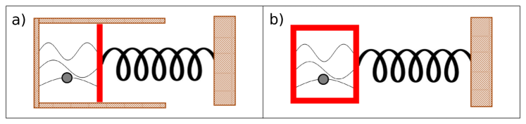
Figure 2: (Color on-line) Schematic of a quantum piston. a) The spring is connected to a wall of the potential in which a quantum particle of mass $m$ is initially confined into the ground state. b) As in a) but now the spring is connected to the whole potential well which moves rigidly. The wave-lines in a) and b) represent the low energy wavefunctions of the quantum particle in the confining potential.

5.3 Energy absorption of a spin in a rotating magnetic field.

As a next example we consider a system of independent spin-$\frac{1}{2}$ in a rotating magnetic field in the xz plane. Here we assume that the magnetic filed is an external parameter whose dynamics is given a priori. First we assume that these spins are isolated and later add a weak coupling to a bath. The Hamiltonian of each of the spins reads

$$H\left(\lambda(t)\right)=-\Delta\left(\cos(\lambda)\,\sigma_{z}+\sin(\lambda)\,\sigma_{x}\right)+H_{SB},$$ (37)

where $H_{SB}$ is the part of the Hamiltonian representing possible coupling to the bath and which does not depend on the angle $\lambda$. The instantaneous eigenstates change during the dynamics described by the protocol $\lambda(t)$ while the energy levels remain unchanged. The eigenstates of this Hamiltonian (excluding the bath) are trivially

$$|gs_{\lambda}\rangle=\left(\begin{array}[]{c}\cos\left(\frac{\lambda}{2}\right)\\ \sin\left(\frac{\lambda}{2}\right)\end{array}\right),\quad|ex_{\lambda}\rangle=\left(\begin{array}[]{c}\sin\left(\frac{\lambda}{2}\right)\\ -\cos\left(\frac{\lambda}{2}\right)\end{array}\right)$$ (38)

corresponding to the energies $E_{gs}=-\Delta$ and $E_{ex}=\Delta$ respectively. It is straightforward to compute the mass $\kappa$ using Eq. (26):

$$\kappa=\frac{\tanh(\beta\Delta)}{4\Delta}\$$ (39)

In the high temperature limit $\kappa\approx\beta/4$, which is indeed a product of the inverse temperature and the single component metric tensor, also known as the fidelity susceptibility of the spin. Because this expression is non-singular, a small coupling to the bath can at most introduce small corrections to $\kappa$. However, this is not the case with dissipative coefficient $\eta$, which clearly vanishes in the long time limit without the bath because there are no gapless excitations. For typical coupling to the bath the transverse spin-spin correlation functions entering Eq. (24) oscillate with frequency $2\Delta$ and decay with the relaxation time $\tau_{c}$ set by the bath [34, 35] so

$$\begin{split}\eta&=\Delta\tanh(\beta\Delta)\int_{0}^{\infty}dt^{\prime}\cos(2\Delta t^{\prime})\exp\left[-\frac{t^{\prime}}{\tau_{c}}\right]\\ &=\tanh(\beta\Delta)\,\frac{\Delta\tau_{c}}{1+(2\Delta\tau_{c})^{2}}\end{split}$$ (40)

Within the same approximation the mass $\kappa$ is also modified:

$$\begin{split}\kappa&=\Delta\tanh(\beta\Delta)\int_{0}^{\infty}dt^{\prime}(-t^{\prime})\cos(2\Delta t^{\prime})\exp\left[-\frac{t^{\prime}}{\tau_{c}}\right]\\ &=\tanh(\beta\Delta)\,\Delta\tau_{c}^{2}\frac{(2\Delta\tau_{c})^{2}-1}{((2\Delta\tau_{c})^{2}+1)^{2}}\end{split}$$ (41)

which reduces to Eq. (39) for $\tau_{c}\Delta\gg 1$. In the high temperature limit $\beta\Delta\ll 1$ this expression for the mass is equal to the inverse temperature times the metric tensor but now of the full system including bath degrees of freedom. These expressions Eq.(40) and (41) do not apply for $\tau_{c}<\Delta^{-1}$ since the simple approximation to the exponentially decaying correlation function breaks in this limit due to the Zeno effect. Therefore we only consider the situation $\Delta\tau_{c}\gg 1$. In Fig. 3 we show the spin energy obtained by numerically integrating the expression $\dot{Q}(t)=\dot{\lambda}(t)\int_{0}^{t}dt^{\prime}\dot{\lambda}(t-t^{\prime})\cos(2\Delta t^{\prime})\exp[-t^{\prime}/\tau_{c}]$ for the protocol $\dot{\lambda}(t)=v_{0}\tanh^{2}(t/\tau_{v})$. Note that $\dot{\lambda}(t)$ starts smoothly and approaches the constant value $v_{0}$ for $t\gtrsim 2\tau_{v}$. For $t<\Delta^{-1}$ the heat $Q(t)$ is well approximated by the short time expansion (see Eq. (30)) while for $\Delta^{-1}<t\lesssim t^{\ast}=\kappa/\eta\approx\tau_{c}$ we observe a plateau in agreement with the general discussion in 3.1.

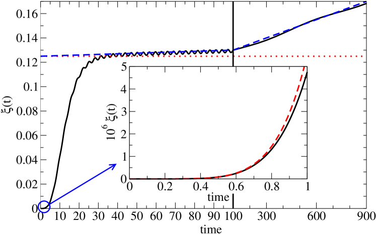
Figure 3: (Color on-line) Rescaled heat, $\xi(t)\equiv\frac{Q(t)}{v_{0}^{2}\Delta\tanh(\beta\Delta)}$, for the protocol $\dot{\lambda}(t)$ discussed in the main text. (Main graph) At long time, $t\gg\tau_{v},\Delta^{-1}$,the heat is well approximated by the sum of the mass renormalization and dissipative contributions (dashed blue line) (see Eq. (11)). The horizontal (dotted red) line is the (constant) contribution from the mass renormalization. (Inset) At short time, $t<\Delta^{-1}$ the heat is well approximated by $Q(t)=\Delta\tanh(\beta\Delta)\frac{(\delta\lambda(t))^{2}}{2}$ (see Eq. 30) (red dashed line). In both panels $\Delta=1,\,\tau_{v}=10,\,\tau_{c}=10^{3}$ so that the condition $\tau_{c}\gg\tau_{v}>\Delta^{-1}$ is well satisfied and the the plateau is well visible.

5.4 Central spin model. Extracting the Chern number from the Coriolis force.

As a third example let us consider a macroscopic rotator (angular momentum) interacting with independent spin-$\frac{1}{2}$ particles. If instead of the rotator we use the quantum spin operator, this model is known as the central spin model. Because dynamics of a spin in any external field is always classical (the evolution of the Wigner function is exactly described by classical trajectories) there is no difference between quantum and classical dynamics in this case and we do not need to assume that the rotator is macroscopic. The Hamiltonian describing the system is (5) with

$$H_{0}=\frac{\vec{L}^{2}}{2I}+V(\vec{n}),\quad H=-\vec{n}\cdot\sum_{i=1}^{N}\Delta_{i}\,\vec{\sigma}_{i},$$ (42)

where $I$ is the momentum of inertia, $V(\vec{n})$ is a time-dependent external potential, $\vec{L}$ is the angular momentum and $\vec{n}$ is the three-dimensional unit vector which can be parameterized using spherical angles: $\vec{n}=(n_{x},n_{y},n_{z})=(\sin\theta\cos\phi,\sin\theta\sin\phi,\cos\theta)$. This example is similar to the previous one except that the effective magnetic field is no longer confined to the $xz$ plane and we no longer assume that it is given by an external protocol. The time evolution of this system needs to be found self-consistently. On the one hand, each spin evolves according to the von Neumann equation with the time-dependent Hamiltonian $H(\vec{n}(t))$:

$$i\partial_{t}\rho=\left[H(\vec{n}(t)),\rho\right]$$ (43)

and, on the other hand, the rotator evolves according to the Hamilton equations of motion

$$I\dot{\vec{n}}=\vec{L}\times\vec{n},\,\quad\dot{\vec{L}}=\vec{n}\times\left(\vec{M}_{ext}+\langle-\frac{\partial H}{\partial\vec{n}}\rangle\right)=\vec{n}\times\left(\vec{M}_{ext}+\sum_{i}\Delta_{i}\langle\vec{\sigma}_{i}\rangle\right)$$ (44)

where $\vec{M}_{ext}=-\frac{\partial V(\vec{n})}{\partial\vec{n}}$ is the external force and $\langle\dots\rangle$ indicates the quantum average over the density matrix $\rho(t)$ (see Eq. (43)). We assume that initially $\vec{n}_{0}=(0,0,1)$ and the spins are in thermal equilibrium with respect the Hamiltonian $H(\vec{n}_{0})$, i.e. $\langle\sigma^{x}_{i}\rangle_{0}=\langle\sigma^{y}_{i}\rangle_{0}=0$ and $\langle\sigma^{z}_{i}\rangle_{0}=\tanh(\beta\Delta_{i})$.

For the toy model proposed here these coupled equations can be easily solved numerically. In fact, according to the Ehrenfest theorem, the evolution of the expectation values follow the classical equation of motion and the von Neumann equation (43) can be replaced with the much simpler equation $\dot{\vec{m}}_{i}=2\Delta_{i}\,\vec{m}_{i}\times\vec{n}$ where $\vec{m_{i}}=\langle\vec{\sigma}_{i}\rangle$. Therefore the exact dynamics of the system consists of the vectors ($\vec{L},\vec{n},\{\vec{m}_{i}\})$ precessing around each other.

We now compare the exact dynamics with the emergent Newton’s law. First, we note that the form of the equations (44) immediately implies

$$\begin{split}&\dot{\vec{n}}\cdot\vec{L}=0,\,\,\vec{n}\cdot\dot{\vec{L}}=0\rightarrow\vec{n}\cdot\vec{L}=\text{const}\\ &\dot{\vec{n}}\cdot\vec{n}=0\rightarrow|\vec{n}|^{2}=\text{const},\,\,\ddot{\vec{n}}\cdot\vec{n}=-|\dot{\vec{n}}|^{2}\end{split}$$ (45)

Next we need to compute the generalized force $\langle\vec{\mathcal{M}}\rangle=\langle-\frac{\partial H}{\partial\vec{n}}\rangle$, and the tensors $\kappa$ and $F$. The drag term $\eta$ and the anti-symmetric mass $F^{\prime}$ are zero since there are no gapless excitations. Therefore Eq. (15) reduces to:

$$\langle\vec{\mathcal{M}}\rangle=\langle\vec{\mathcal{M}}\rangle_{0}+F_{\nu,\mu}\dot{n}_{\mu}-\kappa_{\nu,\mu}\ddot{n}_{\mu}$$

where $\nu,\mu=x,y,z$. The ground and excited states of each spin-$\frac{1}{2}$ are:

$$|gs^{i}_{\theta,\phi}\rangle=\left(\begin{array}[]{c}\cos\left(\frac{\theta}{2}\right)\mathrm{e}^{-i\phi/2}\\ \sin\left(\frac{\theta}{2}\right)\mathrm{e}^{+i\phi/2}\end{array}\right),\quad|ex^{i}_{\theta,\phi}\rangle=\left(\begin{array}[]{c}\sin\left(\frac{\theta}{2}\right)\mathrm{e}^{-i\phi/2}\\ -\cos\left(\frac{\theta}{2}\right)\mathrm{e}^{+i\phi/2}\end{array}\right)$$ (46)

with energy $\pm\Delta_{i}$ respectively from which it follows

$$\langle\vec{\mathcal{M}}\rangle_{0}=0,\quad F=F_{0}\left(\begin{array}[]{ccc}0&n_{z}&-n_{y}\\ -n_{z}&0&n_{x}\\ n_{y}&-n_{x}&0\end{array}\right),$$

$$\kappa=\kappa_{0}\left(\begin{array}[]{ccc}1-n_{x}^{2}&-n_{x}n_{y}&-n_{x}n_{z}\\ -n_{y}n_{x}&1-n_{y}^{2}&-n_{y}n_{z}\\ -n_{z}n_{x}&-n_{z}n_{y}&1-n_{z}^{2}\end{array}\right).$$

where $F_{0}\equiv\frac{1}{2}\sum_{i}\tanh(\beta\Delta_{i})$ and $\kappa_{0}\equiv\sum_{i}\frac{\tanh(\beta\Delta_{i})}{4\Delta_{i}}$. Substituting these expressions in Eq. (44) we find

$$I\dot{\vec{n}}=\vec{L}\times\vec{n},\,\,\dot{\vec{L}}=\vec{n}\times\vec{M}_{ext}+F_{0}\,\dot{\vec{n}}-\kappa_{0}\,(\vec{n}\times\ddot{\vec{n}})$$

where we have used standard properties of the vector triple product together with Eqs. (45). In the equations above we can substitute $\vec{L}\rightarrow\vec{L}_{\perp}$ where by definition $\vec{L}_{\perp}=\vec{L}-(\vec{L}\cdot\vec{n})\vec{n}$. We now compute $I\ddot{\vec{n}}=\dot{\vec{L}}_{\perp}\times\vec{n}+\vec{L}_{\perp}\times\dot{\vec{n}}$ and using standard properties of the vector triple product together with $\vec{L}_{\perp}=I\,(\vec{n}\times\dot{\vec{n}})$ and Eqs. (45) we arrive at:

$$I_{eff}\ddot{\vec{n}}=\left(\vec{n}\times\vec{M}_{ext}\right)\times\vec{n}+F_{0}(\dot{\vec{n}}\times\vec{n})-I_{eff}|\dot{\vec{n}}|^{2}\vec{n}$$ (47)

where we have defined the renormalized momentum of inertia is $I_{eff}=I+\kappa_{0}$.

From this equation we see that the moment of inertia of the rotator is renormalized by the interaction with the spin-$\frac{1}{2}$ particles. Moreover we see that, even when the external force is absent ($\vec{M}_{ext}=0$), the Berry curvature ($F_{0}$) causes the Coriolis type force tilting the rotation plane of the rotator. Indeed if we start with uniform rotations of the rotator in the $xz$ plane, i.e. $\vec{n},\,\dot{\vec{n}}$ lie in the $xz$ plane, we immediately see that the Berry curvature causes acceleration orthogonal to the rotation plane. The physics behind the Coriolis force is intuitively simple. At any finite rotator’s velocity, the spins will not be able to follow adiabatically the rotator and thus will be somewhat behind. As a result there will be a finite angle between the instantaneous direction of the spins and the rotator so the spins will start precessing around the rotator. This precession will result in a finite tilt of the spin orientation with respect to the rotation plane proportional to the Berry curvature [23]. In turn this tilt will result in precession of the rotator around the spins and cause the tilt of the rotation plane. It is interesting that despite the motion of the rotator is completely classical the Coriolis force given by the Berry curvature is quantum in nature. In particular, at zero temperature the integral of the Berry curvature over the closed manifold ($4\pi$ spherical angle is this case) is quantized. Therefore by measuring the Coriolis force and averaging it over the angles $\theta$ and $\phi$ one should be able to accurately see a quantized value:

$$\int_{0}^{\pi}d\theta\int_{0}^{2\pi}d\phi\,F_{\theta,\phi}=2\pi N.$$ (48)

It is interesting that this result remains robust against any small perturbations in the system, which do not close the gap in the spectrum. Similarly the origin of the extra mass (moment of inertia) $\kappa$ in this simple example is purely quantum, i.e. despite this mass describes the classical Newtonian motion, it can not be computed within the classical framework.

We now analyze the approximated Equation (47) in detail. We consider the situation in which $\vec{M}_{ext}(t)$ is slowly turned on (off) at time $t=0$ ($t=t_{c}$). When $\vec{M}_{ext}(t)=0$ Eq. (47) describes a uniform circular motion whose solution can be written as:

$$\vec{n}_{ap}(t)=\sqrt{1-A_{ap}^{2}}\,\,\hat{r}+A_{ap}\,\,\left[\cos(\omega_{ap}t+\phi)\,\,\hat{c}_{1}+\sin(\omega_{ap}t+\phi)\,\,\hat{c}_{2}\right]$$ (49)

where $A_{ap}$ is the amplitude, $\omega_{ap}$ is the angular frequency, $\hat{r}$ is the vector orthogonal to the plane of motion (see Fig. 4) and $\hat{c}_{1}$, $\hat{c}_{2}$ are two orthogonal unit vectors spanning the plane of motion. Substituting the ansatz (49) in Eq. (47) (with $\vec{M}_{ext}=0$) we obtain

$$\omega_{ap}=-\frac{F_{0}}{I_{eff}\sqrt{1-A_{ap}^{2}}}.$$ (50)

The amplitude and the orientation of the plane of motion can not be computed from the initial conditions of Eq. (47) since this equation is only valid after a transient time. We therefore extract them from the exact numerical solution:

$$\sqrt{1-A_{ap}^{2}}\,\,\hat{r}=\lim_{T\rightarrow\infty}\frac{1}{T}\int_{t_{c}}^{t_{c}+T}dt^{\prime}\,\vec{n}_{ex}(t^{\prime})$$

and compute $\omega_{ap}$ via Eq. (50). In Fig. 4 we compare the exact trajectory $\vec{n}_{ex}(t)$ obtained by numerically solving Eq. (43) and Eq. (44) for the rotator coupled to $N=20$ spins with gaps $\Delta_{i}$ uniformly distributed between $(1,2)$ to the approximated trajectory $\vec{n}_{ap}(t)$ (49). We note that the frequency of the approximated motion (estimated via Eq.(50)) underestimates the exact frequency by $8\%$ however if we had used the bare momentum of inertia in (50) with the chosen simulation parameters ($I_{eff}/I\approx 1.5$) we would have overestimated the exact frequency by $28\%$. The accuracy will be higher if we increase the number of spins $N$.

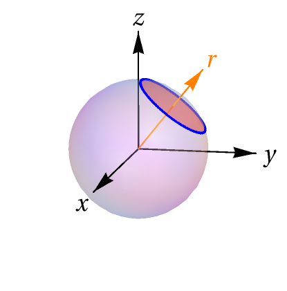
Figure 4: (Color on-line) Dynamics of a rotator coupled to $N=20$ spins-$\frac{1}{2}$. (Left panel) The exact trajectory of the rotator obtained by numerically solving Eq. (43) and (44) (blue line) coincides with the approximated trajectory Eq. (49) which delimits the shaded red plane. (Right panel) Behavior of $n_{z}(t)$ for the exact (continuous blue) and approximated evolution (dashed red) versus time. The parameters of the exact simulations are: $N=20$, $\beta=0.1$, $I=1$, $\Delta_{i}$ are randomly distributed in $(1,2)$. For these parameters $F_{0}\approx 1.5$, $\kappa_{0}\approx 0.5$ and $I_{eff}/I\approx 1.5$. The initial conditions are $\vec{n}_{0}=(0,0,1)$ and $\vec{L}_{0}=(0,0,0)$ and initially the spins are in thermal equilibrium (see main text). We chose the time-dependent external force to be $\vec{M}_{ext}(t)=250\left[\frac{t}{t_{c}}\left(1-\frac{t}{t_{c}}\right)\right]^{4}\,\hat{x}$ for $0\leq t\leq t_{c}=3$ and zero otherwise.

6 Conclusions

In this paper we showed how macroscopic Newtonian dynamics for slow degrees of freedom coupled to an arbitrary system emerges in the leading order of expansion about the adiabatic limit. Our results apply to open and closed systems, quantum and classical. In particular, we found closed microscopic expressions for the friction tensor and for the mass tensor due to dressing of the macroscopic parameter with excitations. We showed that the mass tensor is directly related to the changing geometry of the Hilbert space of the system due to the adiabatic motion of the degree of freedom. In this sense its origin is similar in nature to the origin of the dynamical Casimir force [36, 37]. At a high temperature (or in the classical) limit the mass term becomes equal to the product of the inverse temperature and the Fubini-Study metric tensor describing the system. While we focused on coupling to ergodic systems, which equilibrate at finite temperatures in the absence of motion, our results are more general. In particular, they will apply to non-ergodic, e.g. integrable or glassy systems, as long as they reach some steady state (or approximately steady state). In this case the mass and the friction will be different from the equilibrium values. Thus the mass of the object coupled to a weakly non-integrable system can change in time as the latter slowly equilibrates.

Our results are non perturbative in the coupling between the macroscopic parameter and the (classical or quantum) system and can therefore be applied to situations in which mass renormalization of the macroscopic parameter is large [38]. This is in contrast with the standard many-body Green function approach [19] in which the real and imaginary part of the self energy (which are responsible of the mass renormalization and dissipation respectively) are perturbative in the coupling. Moreover our integral equations  (8) and (14) contain non-Markovian effects and are valid even when the relaxation time in the system is long. Our results are based on the adiabatic perturbation theory which is based on a separation of time-scales between the dynamics of the (slow) macroscopic parameter and the (fast) dynamics of the system [2]. Therefore our approach is different and complementary to the usual Born-Markov scheme of open quantum systems [7, 8, 9].

7 Acknowledgments

We gratefully acknowledge M. Kolodrubetz and E. Katz for many stimulating conversations and M. V. Berry for providing valuable feedback to this work and for pointing to us Ref. [27]. This work was partially supported by BSF 2010318, NSF DMR-0907039, AFOSR FA9550-10- 1-0110

Appendix A Appendix: Microscopic derivation of Eqs. (8) and (14)

Let us show the details of the derivation of Eq. (8) and Eq. (14). We start from the generic Hamiltonian $H(\lambda)$ with eigenstates $|m_{\lambda}\rangle$. Both the Hamiltonian and the eigenstates depend on time through the parameter $\lambda(t)$ which can be multicomponents. For brevity we use the notation $H(t)\equiv H(\lambda(t))$ and $|m_{t}\rangle\equiv|m_{\lambda(t)}\rangle$. Our goal is to compute the evolution of the density matrix $\rho(t)$ subject to the initial condition $\left[\rho^{0},H(\lambda_{0})\right]=0$, i.e. the initial density matrix is stationary with respect the initial Hamiltonian. In the course of our derivation we will implement a sequence of two unitary transformations.

First we make a unitary (time-dependent) transformation, $R(\lambda)$, from the fixed (lab) frame to a new frame which is co-moving with the Hamiltonian. In the following we reserve the tilda sign to the quantities in the co-moving frame. In the co-moving frame the Hamiltonian $\tilde{H}(\lambda)\equiv R^{\dagger}(\lambda)H(\lambda)R(\lambda)$ assumes a diagonal form and its eigenstates $|\tilde{m}\rangle$ are $\lambda$-independent:

$$\langle n_{\lambda}|H(\lambda)|m_{\lambda}\rangle=\langle\tilde{n}|\tilde{H}(\lambda)|\tilde{m}\rangle=\epsilon_{n}(\lambda)\,\delta_{n,m}.$$ (51)

where $|m_{\lambda}\rangle\equiv R(\lambda)|\tilde{m}\rangle$. We note that $|\tilde{m}\rangle=|m_{\lambda_{0}}\rangle$ where $|m_{\lambda_{0}}\rangle$ is the static basis, which diagonalizes the Hamiltonian at the initial value of $\lambda=\lambda_{0}$. In the co-moving frame the wave-function is $|\tilde{\psi}\rangle=R^{\dagger}(\lambda)|\psi\rangle$ and the density matrix is:

$$\tilde{\rho}=R^{\dagger}(\lambda)\rho R(\lambda).$$

We assume that the dynamical process starts at $t=0$ so that $R(0)$ is the identity operator and thus $\rho^{0}$ and $\tilde{\rho}^{0}$ coincide (this condition can be relaxed). The Hamiltonian which governs the time-evolution in the co-moving frame is $\tilde{H}_{eff}$:

$$\tilde{H}_{eff}\equiv\tilde{H}-\dot{\lambda}_{\nu}\tilde{\mathcal{A}}_{\nu}$$ (52)

The first term $\tilde{H}$ is diagonal and it is therefore only responsible for phase accumulation. The second “Galilean” type term (see e.g. Ref. [30]) originates from the fact that the basis transformation, $R(\lambda)$ is time-dependent and plays the role of translation operator in the parameter space [17]. The operator

$$\tilde{\mathcal{A}}_{\nu}(\lambda)\equiv iR^{\dagger}(\lambda)\partial_{\lambda_{\nu}}R(\lambda)$$ (53)

is a gauge potential. Clearly it can be also written as $\mathcal{A}_{\nu}=i\partial_{\lambda_{\nu}}$ in a sense that

$$i\langle n_{\lambda}|\overrightarrow{\partial}_{\lambda_{\nu}}|m_{\lambda}\rangle=\langle\tilde{n}|\tilde{\mathcal{A}}_{\nu}(\lambda)|\tilde{m}\rangle.$$ (54)

Gauge potentials are generally very complicated many-particle operators. For systems coupled to a bath they involve both the system’s and bath’s degrees of freedom as well as the system-bath interactions. In the co-moving basis this term has off-diagonal components and is responsible for the transition between the energy levels.

Before proceeding let us illustrate this formalism with the example used in the main text (see Sec. 5.3). The Hamiltonian in the fixed (lab) frame is:

$$H\left(\lambda\right)=-\Delta\left(\cos(\lambda)\,\sigma_{z}+\sin(\lambda)\,\sigma_{x}\right)$$

with eigenstates

$$|gs_{\lambda}\rangle=\left(\begin{array}[]{c}\cos\left(\frac{\lambda}{2}\right)\\ \sin\left(\frac{\lambda}{2}\right)\end{array}\right),\quad|ex_{\lambda}\rangle=\left(\begin{array}[]{c}-\sin\left(\frac{\lambda}{2}\right)\\ \cos\left(\frac{\lambda}{2}\right)\end{array}\right)$$

The unitary transformation, which diagonalizes the instantaneous Hamiltonian, $H(\lambda)$, is the rotation around the $y$-axis by the angle $\lambda$:

$$R(\lambda)=\exp[-i\frac{\sigma_{y}}{2}\lambda]=\left(\begin{array}[]{cc}\cos\left(\lambda/2\right)&-\sin\left(\lambda/2\right)\\ \sin\left(\lambda/2\right)&\cos\left(\lambda/2\right)\end{array}\right)$$

Note that $R(\lambda_{0}=0)=\text{Identity}$. In the rotated (co-moving) frame we have:

$$\tilde{H}\equiv R^{\dagger}(\lambda)H(\lambda)R(\lambda)=-\Delta\sigma_{z}$$

which is diagonal and (in this case) $\lambda$-independent. The eigenstates are trivially:

$$|\tilde{gs}\rangle=\left(\begin{array}[]{c}1\\ 0\end{array}\right),\quad|\tilde{ex}\rangle=\left(\begin{array}[]{c}0\\ 1\end{array}\right)$$

which are identical to the eigenstates at $\lambda_{0}=0$:

$$|\tilde{gs}\rangle=|gs_{\lambda_{0}}\rangle,\,\,|\tilde{ex}\rangle=|ex_{\lambda_{0}})\rangle$$

Finally the Gauge potential is:

$$\tilde{A}\equiv iR^{\dagger}(\lambda)\left(\partial_{\lambda}R(\lambda)\right)=\frac{\sigma_{y}}{2},$$

which in this example is also $\lambda$-independent. Then Eq. (54) is verified by direct inspection.

Next, to derive Eq. (8) and Eq. (14), we solve the von Neumann’s equation

$$i\frac{d\tilde{\rho}}{dt}=\left[\tilde{H}-\dot{\lambda}_{\nu}\tilde{\mathcal{A}}_{\nu},\tilde{\rho}\right]$$

using standard time-dependent perturbation theory with the Galilean term being the perturbation. The easiest way to do so is to go to the interaction picture (the Heisenberg representation with respect to $\tilde{H}$), where the von Neumann’s equation becomes

$$i\,\frac{d\tilde{\rho}_{H}}{dt}=-\dot{\lambda}_{\nu}\left[\tilde{\mathcal{A}}_{H,\nu}(t),\tilde{\rho}_{H}\right],$$ (55)

which is equivalent to the integral equation

$$\tilde{\rho}_{H}(t)=\tilde{\rho}_{H}(0)+i\int_{0}^{t}dt^{\prime}\dot{\lambda}_{\nu}(t^{\prime})\left[\tilde{\mathcal{A}}_{H,\nu}(t^{\prime}),\tilde{\rho}_{H}(t^{\prime})\right]$$

Note that if the moving Hamiltonian $\tilde{H}$ is time dependent (which is the case when the energy spectrum depends explicitly on $\lambda$, see Eq. (51)) the Heisenberg picture is different from the conventional one. But because $\tilde{H}$ is always diagonal in the co-moving basis the difference appears only in the phase factor:

$$\begin{split}\langle\tilde{n}|\tilde{O}_{H}(\lambda(t))|\tilde{m}\rangle&=\exp\left[i\int_{0}^{t}dt^{\prime}(\epsilon_{n}(t^{\prime})-\epsilon_{m}(t^{\prime}))\right]\langle\tilde{n}|\tilde{O}(\lambda(t))|\tilde{m}\rangle\\ &=\exp\left[i\int_{0}^{t}dt^{\prime}(\epsilon_{n}(t^{\prime})-\epsilon_{m}(t^{\prime}))\right]\langle n_{t}|O(\lambda(t))|m_{t}\rangle\end{split}$$ (56)

which follows from the definition

$$\tilde{O}_{H}(t)\equiv\left(e^{i\int_{0}^{t}\,d\tau\tilde{H}(\tau)}\right)R^{\dagger}(t)O(t)R(t)\left(e^{-i\int_{0}^{t}\,d\tau\tilde{H}(\tau)}\right)$$

We emphasize that this expression is not the same as the Heisenberg representation with respect to the original Hamiltonian $H(\lambda(t))$. The representation we use is perhaps more correctly termed as the adiabatic Heisenberg representation since it uses adiabatic energy levels $\epsilon_{n}(t)$, while all the transitions (off-diagonal terms) are treated perturbatively. Clearly if $\epsilon_{n}$ is time independent the expression (56) reduces to the conventional Heisenberg representation of the operator $O(\lambda(t))$ which can depend on time through the parameter $\lambda(t)$. We can now solve Eq. (55) iteratively to the second order in $\dot{\lambda}$:

$$\begin{split}\partial_{t}\tilde{\rho}_{H}(t)&=i\dot{\lambda}_{\nu}(t)\left[\tilde{\mathcal{A}}_{H,\nu}(t),\rho^{0}\right]\\ &-\dot{\lambda}_{\nu}(t)\int_{0}^{t}dt^{\prime}\dot{\lambda}_{\mu}(t^{\prime})\left[\tilde{\mathcal{A}}_{H,\nu}(t),\left[\tilde{\mathcal{A}}_{H,\mu}(t^{\prime}),\rho^{0}\right]\right]+\mathcal{O}(|\dot{\lambda}|^{3}),\end{split}$$

where we used $\tilde{\rho}_{H}^{0}=\tilde{\rho}^{0}=\rho^{0}$.

To derive Eq. (8) we analyze the energy generation rate

$$\partial_{t}\langle H\rangle=\partial_{t}\left({\rm Tr}\left\{\tilde{\rho}_{H}(t)\,\tilde{H}(t)\right\}\right)=\dot{W}(t)+\dot{Q}(t),$$

where

$$\dot{W}(t)={\rm Tr}\left\{\tilde{\rho}_{H}(t)\,(\partial_{t}\tilde{H})\right\},\;\dot{Q}(t)={\rm Tr}\left\{(\partial_{t}\tilde{\rho}_{H})\,\tilde{H}(t)\right\}$$

The adiabatic work rate, related to the change of the spectrum in the Hamiltonian, in turn can be rewritten as

$$\dot{W}(t)=-\dot{\lambda}_{\nu}M_{\nu}+\mathcal{O}\left(|\dot{\lambda}|^{3}\right),$$

where

$$M_{\nu}=-\sum_{n}\langle n_{0}|\rho^{0}|n_{0}\rangle\left(\partial_{\lambda_{\nu}}\epsilon_{n}(\lambda)\right)\equiv-\langle\partial_{\lambda_{\nu}}H\rangle_{0}\equiv\langle\mathcal{M}_{\nu}\rangle_{0}$$

is the generalized force with respect the initial (stationary) density matrix and we have defined $\mathcal{M}_{\nu}\equiv-\partial_{\lambda_{\nu}}H$. For an initially stationary density matrix, $\left[\rho^{0},H(\lambda_{0})\right]=0$, it is easy to see that $\left[\tilde{\rho}^{0},\partial_{t}\tilde{H}\right]=0$ (recall that $\tilde{H}(t)$ is diagonal for any time $t$) and there is no second order contribution in $\dot{\lambda}$ to the work rate. In general we find that for an initially stationary density matrix the work rate (heat rate) is odd (even) in $\dot{\lambda}$. Then the leading contribution to the heat rate $\dot{Q}$ , related to the change of occupation of the instantaneous eigenstates of the Hamiltonian, is quadratic in $\dot{\lambda}$ and we find

$$\begin{split}\dot{Q}(t)&=-\dot{\lambda}_{\nu}(t)\int_{0}^{t}dt^{\prime}\dot{\lambda}_{\mu}(t^{\prime})\times{\rm Tr}\left\{\tilde{H}(t)\left[\tilde{\mathcal{A}}_{H,\nu}(t),\left[\tilde{\mathcal{A}}_{H,\mu}(t^{\prime}),\rho^{0}\right]\right]\right\}\\ &=\dot{\lambda}_{\nu}(t)\int_{0}^{t}dt^{\prime}\dot{\lambda}_{\mu}(t^{\prime})\,\,\left<\left[\left[\tilde{\mathcal{A}}_{H,\nu}(t),\tilde{H}(t)\right],\tilde{\mathcal{A}}_{H,\mu}(t^{\prime})\right]\right>_{0}\end{split}$$ (57)

Note that in this expression the Hamiltonian $\tilde{H}(t)$ depends on time only through the spectrum and it is diagonal for any time $t$. From the definition of $\tilde{\mathcal{A}}_{\nu}\equiv iR^{\dagger}\left(\partial_{\lambda_{\nu}}R\right)$ and $\tilde{H}\equiv R^{\dagger}HR$ it follows that:

$$\left[\tilde{\mathcal{A}}_{\nu}(t),\tilde{H}(t)\right]=-i\tilde{\mathcal{M}}_{\nu}-i\partial_{\lambda_{\nu}}\tilde{H}$$ (58)

where

$$\tilde{\mathcal{M}}_{\nu}\equiv R^{\dagger}\mathcal{M}_{\nu}R\equiv-R^{\dagger}\left(\partial_{\lambda_{\nu}}H\right)R$$

is the generalized force in the co-moving basis and we have used the identity $\left(\partial_{\lambda_{\nu}}R\right)R^{\dagger}=-R\left(\partial_{\lambda_{\nu}}R^{\dagger}\right)$. Eq. (58) naturally follows from the interpretation of the gauge potential $\mathcal{A}_{\nu}$ as the (negative) momentum operator along the direction $\lambda_{\nu}$: $\mathcal{A}_{\nu}=i\partial_{\lambda_{\nu}}$ (see Eq. (54)). The second term in the RHS of Eq. (58) is diagonal in the co-moving basis and does not contribute to Eq. (57), which then simplifies to

$$\dot{Q}=-i\dot{\lambda}_{\nu}(t)\int_{0}^{t}dt^{\prime}\dot{\lambda}_{\mu}(t^{\prime})\,\,\left<\left[\tilde{\mathcal{M}}_{H,\nu}(t),\tilde{\mathcal{A}}_{H,\mu}(t^{\prime})\right]\right>_{0}$$ (59)

And finally, evaluating this expression in the co-moving basis (see Eq. (56)), and using the identity

$$\langle\tilde{n}|\tilde{\mathcal{A}}_{\mu}(\lambda)|\tilde{m}\rangle=i\langle n_{\lambda}|\partial_{\lambda_{\mu}}|m_{\lambda}\rangle=-i\frac{\langle n_{\lambda}|\mathcal{M}_{\mu}(\lambda)|m_{\lambda}\rangle}{\epsilon_{m}(\lambda)-\epsilon_{n}(\lambda)}=-i\frac{\langle\tilde{n}|\tilde{\mathcal{M}}_{\mu}(\lambda)|\tilde{m}\rangle}{\epsilon_{m}(\lambda)-\epsilon_{n}(\lambda)}$$ (60)

we arrive at

$$\dot{Q}(t)=\dot{\lambda}_{\nu}(t)\int_{0}^{t}dt^{\prime}\,\dot{\lambda}_{\mu}(t^{\prime})$$

$$\times\sum_{n\neq m}\,\frac{\rho_{n}^{0}-\rho_{m}^{0}}{\epsilon_{m}(t^{\prime})-\epsilon_{n}(t^{\prime})}\mathrm{e}^{i\int_{t^{\prime}}^{t}d\tau(\epsilon_{m}(\tau)-\epsilon_{n}(\tau))}\langle m_{t}|\mathcal{M}_{\nu}(\lambda(t))|n_{t}\rangle\langle n_{t^{\prime}}|\mathcal{M}_{\mu}(\lambda(t^{\prime}))|m_{t^{\prime}}\rangle$$

$$=\dot{\lambda}_{\nu}(t)\int_{0}^{t}dt^{\prime}\,\dot{\lambda}_{\mu}(t^{\prime})$$

$$\times\sum_{n\neq m}\,\frac{\rho_{n}^{0}-\rho_{m}^{0}}{\epsilon_{m}(t^{\prime})-\epsilon_{n}(t^{\prime})}\mathrm{e}^{i\int_{t^{\prime}}^{t}d\tau(\epsilon_{m}(\tau)-\epsilon_{n}(\tau))}\langle\tilde{m}|\tilde{\mathcal{M}}_{\nu}(\lambda(t))|\tilde{n}\rangle\langle\tilde{n}|\tilde{\mathcal{M}}_{\mu}(\lambda(t^{\prime}))|\tilde{m}\rangle$$

$$=\dot{\lambda}_{\nu}(t)\int_{0}^{t}dt^{\prime}\,\dot{\lambda}_{\mu}(t^{\prime})\sum_{n\neq m}\,\frac{\rho_{n}^{0}-\rho_{m}^{0}}{\epsilon_{m}(t^{\prime})-\epsilon_{n}(t^{\prime})}\langle\tilde{m}|\tilde{\mathcal{M}}_{H,\nu}(t)|\tilde{n}\rangle\langle\tilde{n}|\tilde{\mathcal{M}}_{H,\mu}(t^{\prime})|\tilde{m}\rangle$$

$$=\dot{\lambda}_{\nu}(t)\int_{0}^{t}dt^{\prime}\,\int_{0}^{\beta}\,d\tau\,\,\dot{\lambda}_{\mu}(t^{\prime})\sum_{n\neq m}\,\rho_{m}^{0}\langle\tilde{m}|\tilde{\mathcal{M}}_{H,\nu}(t)|\tilde{n}\rangle\langle\tilde{n}|\tilde{\mathcal{M}}_{H,\mu}(t^{\prime}+i\tau)|\tilde{m}\rangle$$

$$=\dot{\lambda}_{\nu}(t)\int_{0}^{t}dt^{\prime}\,\int_{0}^{\beta}\,d\tau\,\,\dot{\lambda}_{\mu}(t^{\prime})\,\,\langle\tilde{\mathcal{M}}_{H,\nu}(t)\tilde{\mathcal{M}}_{H,\mu}(t^{\prime}+i\tau)\rangle_{0},$$ (61)

Eq. (61) gives the microscopic heat production rate in the most general form and in the last two lines we have used the fact that, for thermal distribution, $\rho^{0}_{m}=Z^{-1}\exp[-\beta\epsilon_{m}]$, we have

$$\int_{0}^{\beta}\,d\tau\,\,\rho^{0}_{m}\,\,e^{-(\epsilon_{n}-\epsilon_{m})\tau}=\frac{\rho^{0}_{n}-\rho^{0}_{m}}{\epsilon_{m}-\epsilon_{n}}$$ (62)

The derivation of Eq. (14) is even simpler since it requires only going to the first order perturbation theory:

$$\tilde{\rho}_{H}(t)\approx\rho_{0}+i\int_{0}^{t}dt^{\prime}\,\dot{\lambda}_{\mu}(t^{\prime})\left[\tilde{\mathcal{A}}_{H,\mu}(t^{\prime}),\rho_{0}\right].$$ (63)

Therefore

$$\langle\mathcal{M}_{\nu}(t)\rangle=M_{\nu}(t)+i\int_{0}^{t}dt^{\prime}\,\dot{\lambda}_{\mu}(t^{\prime})\langle[\tilde{\mathcal{M}}_{H,\nu}(t),\tilde{\mathcal{A}}_{H,\mu}(t^{\prime})]\rangle_{0},$$

where we recall that by definitions $M_{\nu}(t)\equiv\langle\mathcal{M}_{\nu}(t)\rangle_{0}$. Evaluating this expression in the co-moving basis (see Eq. (56)) and using the identity (60) we arrive at

$$\langle\mathcal{M}_{\nu}(t)\rangle=M_{\nu}(t)-\int_{0}^{t}dt^{\prime}\,\dot{\lambda}_{\mu}(t^{\prime})$$

$$\times\sum_{n\neq m}\,\frac{\rho_{n}^{0}-\rho_{m}^{0}}{\epsilon_{m}(t^{\prime})-\epsilon_{n}(t^{\prime})}\mathrm{e}^{i\int_{t^{\prime}}^{t}d\tau(\epsilon_{m}(\tau)-\epsilon_{n}(\tau))}\langle m_{t}|\mathcal{M}_{\nu}(\lambda(t))|n_{t}\rangle\langle n_{t^{\prime}}|\mathcal{M}_{\mu}(\lambda(t^{\prime}))|m_{t^{\prime}}\rangle$$

$$=M_{\nu}(t)-\int_{0}^{t}dt^{\prime}\,\dot{\lambda}_{\mu}(t^{\prime})$$

$$\times\sum_{n\neq m}\,\frac{\rho_{n}^{0}-\rho_{m}^{0}}{\epsilon_{m}(t^{\prime})-\epsilon_{n}(t^{\prime})}\mathrm{e}^{i\int_{t^{\prime}}^{t}d\tau(\epsilon_{m}(\tau)-\epsilon_{n}(\tau))}\langle\tilde{m}|\tilde{\mathcal{M}}_{\nu}(\lambda(t))|\tilde{n}\rangle\langle\tilde{n}|\tilde{\mathcal{M}}_{\mu}(\lambda(t^{\prime}))|\tilde{m}\rangle$$

$$=M_{\nu}(t)-\int_{0}^{t}dt^{\prime}\,\dot{\lambda}_{\mu}(t^{\prime})\sum_{n\neq m}\,\frac{\rho_{n}^{0}-\rho_{m}^{0}}{\epsilon_{m}(t^{\prime})-\epsilon_{n}(t^{\prime})}\langle\tilde{m}|\tilde{\mathcal{M}}_{H,\nu}(t)|\tilde{n}\rangle\langle\tilde{n}|\tilde{\mathcal{M}}_{H,\mu}(t^{\prime})|\tilde{m}\rangle$$

$$=M_{\nu}(t)-\int_{0}^{t}dt^{\prime}\int_{0}^{\beta}\,d\tau\,\,\dot{\lambda}_{\mu}(t^{\prime})\sum_{n\neq m}\,\rho_{m}^{0}\langle\tilde{m}|\tilde{\mathcal{M}}_{H,\nu}(t)|\tilde{n}\rangle\langle\tilde{n}|\tilde{\mathcal{M}}_{H,\mu}(t^{\prime}+i\tau)|\tilde{m}\rangle$$

$$=M_{\nu}(t)-\int_{0}^{t}dt^{\prime}\int_{0}^{\beta}d\tau\,\,\dot{\lambda}_{\mu}(t^{\prime})\langle\tilde{\mathcal{M}}_{H,\nu}(t)\tilde{\mathcal{M}}_{\mu}(t^{\prime}+i\tau)\rangle_{0},$$ (64)

which gives the microscopic force in the most general form.

In Eqs. (61) and (64) we now perform a change of dummy integration variable $t^{\prime}\rightarrow t-t^{\prime}$ and observe that the leading order in $|\dot{\lambda}|$ corresponds to evaluate the spectrum, the eigenstates and the force at the final time of the evolution, i.e. at $t^{\prime}=0$. This is because the energies, the forces and the eigenstates depend on time only through the parameter $\lambda(t)$ and can therefore be expanded in powers of $|\dot{\lambda}|$. For example

$$\epsilon_{m}(t-t^{\prime})\equiv\epsilon_{m}(\lambda(t-t^{\prime}))=\epsilon_{m}(t)-t^{\prime}\dot{\lambda}(t)\partial_{\lambda}\epsilon_{m}+\dots\approx\epsilon_{m}(t)$$

We then obtain the leading contributions:

$$\dot{Q}(t)=\dot{\lambda}_{\nu}(t)\int_{0}^{t}dt^{\prime}\,\dot{\lambda}_{\mu}(t-t^{\prime})$$

$$\times\sum_{n\neq m}\,\,e^{i(\epsilon_{m}(t)-\epsilon_{n}(t))t^{\prime}}\frac{\rho_{n}^{0}-\rho_{m}^{0}}{\epsilon_{m}(t)-\epsilon_{n}(t)}\langle m_{t}|\mathcal{M}_{\nu}(\lambda(t))|n_{t}\rangle\langle n_{t}|\mathcal{M}_{\mu}(\lambda(t))|m_{t}\rangle$$ (65)

$$\langle\mathcal{M}_{\nu}(t)\rangle=M_{\nu}(t)-\int_{0}^{t}dt^{\prime}\,\dot{\lambda}_{\mu}(t-t^{\prime})$$

$$\times\sum_{n\neq m}e^{i(\epsilon_{m}(t)-\epsilon_{n}(t))t^{\prime}}\frac{\rho_{n}^{0}-\rho_{m}^{0}}{\epsilon_{m}(t)-\epsilon_{n}(t)}\langle m_{t}|\mathcal{M}_{\nu}(\lambda(t))|n_{t}\rangle\langle n_{t}|\mathcal{M}_{\mu}(\lambda(t))|m_{t}\rangle$$ (66)

which for time independent spectrum, $\epsilon_{m}(\lambda(t))=\epsilon_{m}$, and time independent force, $\mathcal{M}_{\mu}(\lambda(t))=\mathcal{M}_{\mu}$ can be rewritten as the equations in the main text (see Eqs. (8) and (14)):

$$\begin{split}\dot{Q}(t)&=\dot{\lambda}_{\nu}(t)\int_{0}^{t}dt^{\prime}\,\int_{0}^{\beta}\dot{\lambda}_{\mu}(t-t^{\prime})\langle\mathcal{M}_{H,\nu}(t^{\prime})\mathcal{M}_{H,\mu}(i\tau)\rangle_{0}\\ \langle\mathcal{M}_{\nu}\rangle&=M_{\nu}-\int_{0}^{t}dt^{\prime}\,\int_{0}^{\beta}\dot{\lambda}_{\mu}(t-t^{\prime})\langle\mathcal{M}_{H,\nu}(t^{\prime})\mathcal{M}_{H,\mu}(i\tau)\rangle_{0}\end{split}$$ (67)

where we have used the fact that, for thermal distribution, $\rho^{0}_{m}=Z^{-1}\exp[-\beta\epsilon_{m}]$, we have

$$\int_{0}^{\beta}\,d\tau\,\,\rho^{0}_{m}\,\,e^{-(\epsilon_{n}-\epsilon_{m})\tau}=\frac{\rho^{0}_{n}-\rho^{0}_{m}}{\epsilon_{m}-\epsilon_{n}}$$

The expressions (67) are correct even if the spectrum and force are time dependent but vary slowly on the scale of the relaxation time in the system.

Appendix B Appendix: General structure of expansion of Eq. (8) and Eq. (14) in time derivatives of $\vec{\lambda}$

Here we analyze the full Taylor expansion of Eq. (8) and and Eq. (14), which we rewrite in the Lehmann’s representation (see Eq. (66)). In order for the following expansion to be valid both the velocity and the energy spectrum need to change slowly compared to the relaxation time scale on the system, i.e. the relaxation time must be the shortest time scale. For times $t$ longer than the relaxation time we can set the upper limit of integration in Eq. (66) to infinity, i.e. $t\to\infty$. Expanding $\dot{\lambda_{\mu}}(t-t^{\prime})$ into the Taylor series

$$\dot{\lambda_{\mu}}(t-t^{\prime})=\sum_{k=1}^{\infty}\lambda_{\mu}^{(k)}(t)\frac{(-t^{\prime})^{k-1}}{(k-1)!}$$

we find:

$$\begin{split}\dot{Q}(t)&=\dot{\lambda}_{\nu}(t)\left(\sum_{k=1}^{\infty}\,\chi_{\nu,\mu}^{k}(t)\,\lambda_{\mu}^{(k)}(t)\right)\\ \langle\mathcal{M}_{\nu}(t)\rangle&=M_{\nu}(t)-\sum_{k=1}^{\infty}\,\chi_{\nu,\mu}^{k}(t)\,\lambda_{\mu}^{(k)}(t)\end{split}$$ (68)

where we have defined:

$$\chi_{\nu,\mu}^{k}(t)\equiv\int_{0}^{\infty}dt^{\prime}\,\frac{(-t^{\prime})^{k-1}}{(k-1)!}\sum_{n\neq m}\mathrm{e}^{i(\epsilon_{m}(t)-\epsilon_{n}(t))t^{\prime}-|\varepsilon|t^{\prime}}\times\\ \frac{\rho_{n}^{0}-\rho_{m}^{0}}{\epsilon_{m}(t)-\epsilon_{n}(t)}\,\langle m_{t}|\mathcal{M}_{\nu}(\lambda(t))|n_{t}\rangle\langle n_{t}|\mathcal{M}_{\mu}(\lambda(t))|m_{t}\rangle$$ (69)

and we have added an infinitesimal imaginary energy $|\varepsilon|$ for convergence. Performing time integration over $t^{\prime}$ we immediately find:

$$\chi_{\nu,\mu}^{k}(t)=\sum_{n\neq m}\frac{(-1)^{k}}{\left(|\varepsilon|+i(\epsilon_{n}(t)-\epsilon_{m}(t))\right)^{k}}\,\times\\ \frac{\rho_{n}^{0}-\rho_{m}^{0}}{\epsilon_{n}(t)-\epsilon_{m}(t)}\langle m_{t}|\mathcal{M}_{\nu}(\lambda(t))|n_{t}\rangle\langle n_{t}|\mathcal{M}_{\mu}(\lambda(t))|m_{t}\rangle$$ (70)

Using the identities

$$\frac{1}{|\varepsilon|+ix}=\pi\delta(x)-\frac{i}{x},\quad\frac{1}{(|\varepsilon|+ix)^{2}}=i\pi\delta^{\prime}(x)-\frac{1}{x^{2}}$$ (71)

eq. (70) can be used to write explicitly the Lehmann representation of the tensors $\eta$, $\kappa$, $F$ and $F^{\prime}$:

$$\begin{split}&\eta_{\nu,\mu}(t)\equiv\frac{\chi_{\nu,\mu}^{1}(t)+\chi_{\mu,\nu}^{1}(t)}{2},\quad F_{\nu,\mu}(t)\equiv-\frac{\chi_{\nu,\mu}^{1}(t)-\chi_{\mu,\nu}^{1}(t)}{2}\\ &\kappa_{\nu,\mu}(t)\equiv\frac{\chi_{\nu,\mu}^{2}(t)+\chi_{\mu,\nu}^{2}(t)}{2},\quad F^{\prime}_{\nu,\mu}(t)\equiv\frac{\chi_{\nu,\mu}^{2}(t)-\chi_{\mu,\nu}^{2}(t)}{2}\end{split}$$

The extra minus sign in the definition of $F_{\nu,\mu}$ is conventional and it is chosen to reproduce known expression for the Berry curvature.

To shorten the notation we now drop the time label but in all the following expressions the energy, the force and the eigenstates should be understood as (slowly) depending on time through the parameter $\lambda(t)$. Equation (70) can be rewritten as

$$\chi_{\nu,\mu}^{k}=\int_{-\infty}^{\infty}d\omega\,\sum_{n\neq m}\,\delta(\epsilon_{n}-\epsilon_{m}-\omega)\frac{(-1)^{k}}{\left(|\varepsilon|+i\omega)\right)^{k}}\frac{\rho_{n}^{0}-\rho_{m}^{0}}{\omega}\langle m|\mathcal{M}_{\nu}|n\rangle\langle n|\mathcal{M}_{\mu}|m\rangle.$$

Expressing

$$\delta(\epsilon_{n}-\epsilon_{m}-\omega)=\int_{-\infty}^{\infty}\frac{dt}{2\pi}\,\mathrm{e}^{-i(\epsilon_{n}-\epsilon_{m}-\omega)t}$$

we obtain the compact expression:

$$\chi_{\nu,\mu}^{k}=-\int_{-\infty}^{\infty}d\omega\,\frac{(-1)^{k}}{\left(|\varepsilon|+i\omega)\right)^{k}}\,\left(\frac{\mathcal{S}_{\nu,\mu}(\omega)}{\omega}\right)$$ (72)

where we have defined the spectral density $\mathcal{S}_{\nu,\mu}(t)$ and its Fourier Transform:

$$\begin{split}\mathcal{S}_{\nu,\mu}(t)&\equiv\frac{1}{2\pi}\,\langle\left[\mathcal{M}_{H,\nu}(t),\mathcal{M}_{H,\mu}(0)\right]\rangle_{0}\\ \mathcal{S}_{\nu,\mu}(\omega)&\equiv\int_{-\infty}^{\infty}dt\,\mathrm{e}^{i\omega t}\,\mathcal{S}_{\nu,\mu}(t)\end{split}$$

From the Lehmann representation

$$\mathcal{S}_{\nu,\mu}(\omega)=-\sum_{n\neq m}\delta(\epsilon_{n}-\epsilon_{m}-\omega)(\rho_{n}^{0}-\rho_{m}^{0})\langle m|\mathcal{M}_{\nu}|n\rangle\langle n|\mathcal{M}_{\mu}|m\rangle$$

it is clear that

$$\mathcal{S}_{\nu,\mu}(\omega)=-\mathcal{S}_{\mu,\nu}(-\omega)$$ (73)

Moreover the fluctuation-dissipation relation can be written as

$$\Phi_{\nu,\mu}(\omega)=\coth\left(\frac{\beta\omega}{2}\right)\mathcal{S}_{\nu,\mu}(\omega)$$

where we have defined

$$\begin{split}\Phi_{\nu,\mu}(\omega)&\equiv\frac{1}{2\pi}\int_{-\infty}^{\infty}dt\,\mathrm{e}^{i\omega t}\,\langle\left\{\mathcal{M}_{H,\nu}(t),\mathcal{M}_{H,\mu}(0)\right\}\rangle_{0}\\ &=\sum_{n\neq m}\delta(\epsilon_{n}-\epsilon_{m}-\omega)(\rho_{n}^{0}+\rho_{m}^{0})\langle m|\mathcal{M}_{\nu}|n\rangle\langle n|\mathcal{M}_{\mu}|m\rangle\end{split}$$

which satisfy the symmetry relation

$$\Phi_{\nu,\mu}(\omega)=\Phi_{\mu,\nu}(-\omega).$$

Finally using the identities (71) we obtain:

$$\begin{split}\chi_{\nu,\mu}^{1}&=\pi\sum_{n\neq m}\,\frac{\rho_{n}^{0}-\rho_{m}^{0}}{\epsilon_{m}-\epsilon_{n}}\langle m|\mathcal{M}_{\nu}|n\rangle\langle n|\mathcal{M}_{\mu}|m\rangle\,\delta(\epsilon_{n}-\epsilon_{m})\\ &+i\sum_{n\neq m}\,\frac{\rho_{n}^{0}-\rho_{m}^{0}}{(\epsilon_{n}-\epsilon_{m})^{2}}\langle m|\mathcal{M}_{\nu}|n\rangle\langle n|\mathcal{M}_{\mu}|m\rangle\\ &=\pi\mathcal{G}_{\nu,\mu}(\omega=0)-i\mathcal{P}\int_{-\infty}^{+\infty}d\omega\,\frac{\mathcal{S}_{\nu,\mu}(\omega)}{\omega^{2}}\\ &=\frac{\pi}{2}\left(\mathcal{G}_{\nu,\mu}(\omega=0)+\mathcal{G}_{\mu,\nu}(\omega=0)\right)-\frac{i}{2}\mathcal{P}\int_{-\infty}^{+\infty}\frac{d\omega}{\omega^{2}}\,\left(\mathcal{S}_{\nu,\mu}(\omega)-\mathcal{S}_{\mu,\nu}(\omega)\right)\\ \chi_{\nu,\mu}^{2}&=i\pi\sum_{n\neq m}\,\frac{\rho_{n}^{0}-\rho_{m}^{0}}{\epsilon_{n}-\epsilon_{m}}\langle m|\mathcal{M}_{\nu}|n\rangle\langle n|\mathcal{M}_{\mu}|m\rangle\,\delta^{\prime}(\epsilon_{n}-\epsilon_{m})\\ &+\sum_{n\neq m}\,\frac{\rho_{n}^{0}-\rho_{m}^{0}}{(\epsilon_{m}-\epsilon_{n})^{3}}\langle m|\mathcal{M}_{\nu}|n\rangle\langle n|\mathcal{M}_{\mu}|m\rangle\\ &=i\pi\partial_{\omega}\mathcal{G}_{\nu,\mu}|_{\omega=0}+\mathcal{P}\int_{-\infty}^{+\infty}d\omega\,\frac{\mathcal{S}_{\nu,\mu}(\omega)}{\omega^{3}}\\ &=\frac{i\pi}{2}\left(\partial_{\omega}\mathcal{G}_{\nu,\mu}|_{\omega=0}-\partial_{\omega}\mathcal{G}_{\mu,\nu}|_{\omega=0}\right)+\frac{1}{2}\mathcal{P}\int_{-\infty}^{+\infty}\frac{d\omega}{\omega^{3}}\,\left(\mathcal{S}_{\nu,\mu}(\omega)+\mathcal{S}_{\mu,\nu}(\omega)\right)\end{split}$$

where $\mathcal{P}$ indicates the principal value, used the symmetry of $\mathcal{S}$ (see Eq. (73)) and we have defined the auxiliary function $\mathcal{G}_{\nu,\mu}(\omega)\equiv\frac{\mathcal{S}_{\nu,\mu}(\omega)}{\omega}=\mathcal{G}_{\mu,\nu}(-\omega)$.

We note that:

$$F_{\nu,\mu}\equiv i\langle\overleftarrow{\partial}_{\lambda_{\nu}}\overrightarrow{\partial}_{\lambda_{\mu}}-\overleftarrow{\partial}_{\lambda_{\mu}}\overrightarrow{\partial}_{\lambda_{\nu}}\rangle_{0}$$

and that when the occupations are thermal we can write:

$$\begin{split}&\eta_{\nu,\mu}=\pi\beta\sum_{n\neq m}\,\rho_{m}^{0}\langle m|\mathcal{M}_{\nu}|n\rangle\langle n|\mathcal{M}_{\mu}|m\rangle\,\delta(\epsilon_{n}-\epsilon_{m})\\ &F^{\prime}=-i\pi\sum_{n\neq m}\,\rho_{m}^{0}\,\left[\beta^{2}\langle m|\mathcal{M}_{\nu}|n\rangle\langle n|\mathcal{M}_{\mu}|m\rangle\right.\\ &-\left.\beta\frac{\partial}{\partial(\epsilon_{n}-\epsilon_{m})}\left(\langle m|\mathcal{M}_{\nu}|n\rangle\langle n|\mathcal{M}_{\mu}|m\rangle\right)\right]\,\delta(\epsilon_{n}-\epsilon_{m}).\end{split}$$

Finally we note that both $\chi^{1}$ and $\chi^{2}$ have a symmetric (under $\nu\leftrightarrow\mu$) and anti-symmetric terms. For $\chi^{1}$ the symmetric part is on-shell and the anti-symmetric part is off-shell. The situation is opposite for $\chi^{2}$. In general, the on-shell terms describe dissipation and vanish for gapped system and zero temperature while the off-shell terms describe the renormalization of the systems’ parameters. For system with time-reversal symmetry all anti-symmetric contributions vanish [25] and, as a result, all odd susceptibilities are dissipative and on-shell while all the even susceptibilities are off-shell and describe renormalization of systems’ parameters. These findings generalize the result of Berry and Robbins [2]. Finally we note that all susceptibilities change sign with the temperature and that for positive temperature ($\beta>0$) the macroscopic degrees of freedom loses energy to the environment in all orders in the derivatives of $\vec{\lambda}(t)$.

References

- [1] F. Wilczek, Physics Today 57, 11 (2004)
- [2] M. V. Berry and J. M. Robbins, Proc. R. Soc. Lond. A 442, 659-672 (1993)
- [3] C. Jarzynski, Phys. Rev. Lett. 74, 2937-2940 (1995)
- [4] J. E. Avron, M. Fraas, G. M. Graf and O. Kenneth, New J. Phys. 13, 053042 (2011)
- [5] R. P. Feynman, Phys. Rev. 94, 262 (1954)
- [6] A. Caldeira and A. J. Leggett, Phys. Rev. Lett. 46, 211-214 (1981)
- [7] G. Lindblad, Commun. Math. Phys. 48, 119-130 (1976)
- [8] G. M. Moy, J. J. Hope and C. M. Savage, Phys. Rev. A 59, 667-675 (1999)
- [9] H.P. Breuer and F. Petruccione, Theory of open quantum systems (Oxford, 2003)
- [10] M. Schecter, D.M. Gangardt, and A. Kamenev, Ann. Phys. (N.Y.) 327, 639 (2012)
- [11] L. D. Landau and E. M. Lifshitz, Statistical Mechanics, part 2 (Butterworth-Heinemann, 1980)
- [12] P. Phillips, Advanced Solid State Physics (Cambridge-University Press, 2008)
- [13] R. Kubo, J. Phys. Soc. Jpn. 12, 570 (1957)
- [14] D. A. Sivak and G. E. Crooks, Phys. Rev. Lett. 108, 190602 (2012).
- [15] J. Provost and G. Vallee, Comm. Math. Phys. 76, 289 (1980).
- [16] L. Campos Venuti and P. Zanardi, Phys. Rev. Lett. 99, 095701 (2007).
- [17] M. Kolodrubetz, V. Gritsev and A. Polkovnikov, arXiv:1305.0568
- [18] Because we are taking the expectation value with the time-dependent density matrix there will be corrections to the generalized force. However, one can show that these corrections are of the order of , which is beyond the accuracy considered in this paper.
- [19] G. Mahan, Many-Particle Physics, 3rd edition (Springer, 2000).
- [20] The minus signs are conventional. The sign of is chosen to reproduce known expressions for the Berry curvature.
- [21] N. Bode, S. Viola Kusminskiy, R. Egger and F. von Oppen, Phys. Rev. Lett. 107, 036804 (2011)
- [22] M. Thomas, T. Karzig, S. Viola Kusminskiy, G. Zarand and F. von Oppen, Phys. Rev. B 86, 195419 (2012)
- [23] V. Gritsev and A. Polkovnikov, Proc. Nat. Acad. USA 109, 6457 (2012)
- [24] H. M. Price and N. R. Cooper, arXiv:1306.4796 [cond-mat.quant-gas]
- [25] Using the Lehmann representation it is easy to write the antisymmetric tensors as differences of two-time correlation functions evaluated at . For system with time-reversal symmetry these correlation functions are identical and all antisymmetric tensors must vanish identically.
- [26] A. Polkovnikov and V. Gritsev, Nature Phys. 4, 477 (2008)
- [27] M. V. Berry, The quantum phase, five years after in “Geometric Phases in Physics”, eds: A Shapere, F Wilczek. (World Scientific) 7-28 (1989).
- [28] M. Campisi, S. Denisov and P. Hänggi, Phys. Rev. A 86, 032114 (2012)
- [29] P. R. Zulkowski, D. A. Sivak, G. E. Crooks, M. R. DeWeese, Phys. Rev. E. 86 0141148 (2012)
- [30] C. De Grandi, A. Polkovnikov, A. Sandvik, arXiv:1301.2329.
- [31] G. E. Crooks, Phys. Rev. Lett. 99, 100602 (2007)
- [32] G. Ruppeiner, Phys. Rev. A 20, 1608 (1979)
- [33] To obtain we need to assume that there are oscillators with vanishingly small frequencies .
- [34] S. Genway, A.F. Ho, D.K.K. Lee, Phys. Rev. Lett. 111, 130408 (2013).
- [35] L. D’Alessio and A. Polkovnikov, unpublished
- [36] G. T. Moore, J. Math. Phys. 11, 2679 (1970)
- [37] C.M. Wilson, G. Johansson, A. Pourkabirian, J.R. Johansson, T. Duty, F. Nori, P. Delsing, Nature 479, 376-379 (2011)
- [38] T. Yefsah, A. T. Sommer, M. J. H. Ku, L. W. Cheuk, W. Ji, W. S. Bakr and M. W. Zwierlin, Nature 499, 426 (2013) connected correlation exponentially, which is usually the case except near singularities like phase transitions.