Sudden Decoherence Transitions for Quantum Discord

Abstract

We investigate the disappearance of discord in 2- and multi-qubit systems subject to decohering influences. We formulate the computation of quantum discord and quantum geometric discord in terms of the generalized Bloch vector, which gives useful insights on the time evolution of quantum coherence for the open system, particularly the comparison of entanglement and discord. We show that the analytical calculation of the global geometric discord is NP-hard in the number of qubits, but a similar statement for global entropic discord is more difficult to prove. We present an efficient numerical method to calculating the quantum discord for a certain important class of multipartite states. In agreement with previous work for 2-qubit cases, (Mazzola et al., Phys. Rev. Lett. 104, 200401 (2010)), we find situations in which there is a sudden transition from classical to quantum decoherence characterized by the discord remaining relatively robust (classical decoherence) until a certain point from where it begins to decay quickly whereas the classical correlation decays more slowly (quantum decoherence). However, we find that as the number of qubits increases, the chance of this kind of transition occurring becomes small.

Keywords: quantum discord, quantum entanglement, quantum decoherence, sudden transition, injective tensor norm, NP-hard problem

1 Introduction

Entanglement is a unique property of composite quantum systems. It is known to be essential for certain quantum communication protocols [1, 2], and it is generally felt to be an essential resource of the exponential speedup of quantum algorithms [3, 4]. For instance, the Deutsch-Josza algorithm (DJA) (the simplest of all quantum algorithms) [5] is designed to figure out if a given function is balanced or not.  Entanglement is unavoidable in the DJA as the number $n$ of qubit increases [6], since the total number of balanced functions scales doubly exponentially: $B(2^{n},2^{n-1})\sim 2^{2^{n}}$, while the number of separable states scales as $2^{n}$. Thus, in order to represent all the balanced function with $n$ qubits, we inevitably introduce entanglement.

On the other hand, there have been questions concerning whether entanglement is the only resource of the power of quantum algorithms [7, 8].  The DJA for the 2- and 3- qubit cases have an advantage over classical algorithm but they do not involve much more than simple interference, not usually thought of as quantum correlation.  Quantum discord has been introduced as another type of quantum correlation [9] that can be present even in separable states.  It might be an additional resource of quantum algorithms giving computational advantages over classical calculation.  Evidence for this point of view comes from the existence of an algorithm (DQC1) that computes the trace of a unitary matrix.  It uses only one pure qubit and exhibits discord but little entanglement [10, 11, 12], and still appears to be more powerful than classical algorithms for the same problem. Since quantum discord is more robust against decoherence than entanglement there is the hope that quantum algorithms dependent only on quantum discord might be more feasible to implement physically than those dependent on the more fragile entanglement.  The true physical resource of quantum computation still has many open issues.

Quantum discord was originally suggested as a quantum measure of correlations between two systems that is analogous to the classical notion of mutual information between two probability distributions in classical information theory.  It can be given an operational meaning as well [13, 14].  The original quantum discord was defined only for bipartite states.  For 2-qubit systems, it has been shown that quantum discord can undergo a transition between quantum and classical decoherence as a function of time on certain physically plausible dynamical trajectories[15, 16, 43, 44].

Our chief focus in this paper is on multipartite systems.  For this purpose, the global quantum discord [17] is defined using distance measures to the nearest classical state. The distance can be defined either by the relative entropy measure [18], or by means of the metric derived from the Hilbert-Schimdt inner product [19, 20, 21]. We will use the latter form in this work, and it is called geometric global quantum discord (GGQD). It facilitates the calculations by removing the nonpolynomial log function from the definition, but at the cost of muddying the information-theoretic interpretation.

The structure of the paper is as follows. The next section briefly introduces the various measures of discord and elucidates their physical meaning. The third section gives an interpretation of quantum discord in terms of Bloch vector geometry, a proof that computing GGCD is NP-hard in the number of qubits, and also treats the problem of 2,3, and N qubits from an algebraic point of view. The fourth section describes a relatively simple heuristic method to calculate GGQD for certain highly symmetric but important classes of multiqubit states, which in turn suggests a condition to obsesrve sudden transition between classical and quantum decoherence [15, 16] in the multiqubit case. This condition appears to be very stringent, meaning that such transitions are not likely to be observed on physical trajectories.

2 Measures of quantum correlation

A good measure of the classical correlation between two probability distributions $\{p_{1,i}\},\{p_{2,j}\}$ with $\{p_{12,ij}\}$ as their joint distribution is given by the mutual information $I_{classical}=H(\{p_{1,i}\})+H(\{p_{2,j}\})-H(\{p_{12,ij}\})$ where $H(\{p_{k}\})\equiv-\sum_{k}p_{k}\log_{2}(p_{k})$ is Shannon entropy. Note that $H(\{p_{12,ij}\})=H(\{p_{1,i}\})+H(\{p_{2,j}\})$ when two distributions are independent so that $I_{classical}=0$. $I_{classical}$ can also be written as

$$I_{classical}=H(\{p_{1,i}\})+H(\{p_{2,j}\})-H(\{p_{12,ij}\})$$

$$=H(\{p_{1,i}\})-(H(\{p_{12,ij}\})-H(\{p_{2,j}\}))$$ (1)

$$=H(\{p_{1,i}\})-\left(-\sum_{ij}p_{12,ij}\log_{2}\left(p_{12,ij}\right)+\sum_{ij}p_{12,ij}\log_{2}(p_{2,i})\right)$$

$$=H(\{p_{1,i}\})-\left(-\sum_{ij}p_{2,j}\left(\frac{p_{12,ij}}{p_{2,j}}\right)\log_{2}(\frac{p_{12,ij}}{p_{2,j}})\right)$$

$$=H\left(\left\{p_{1,i}\right\}\right)-\sum_{j}p_{2,j}H\left(\left\{p_{1|2=j,i}\right\}\right)$$ (2)

Here the conditional probability $p_{1|2=j,i}$ is the probability of event $i$ in system 1, given that event $j$ has been measured in system 2.

This process can be viewed as the partial elimination of uncertainty of system 1 from knowledge of system 2. The classical correlation between two quantum systems can be defined in the light of these equations. In the quantum case, the probability distribution is replaced by the density operator $\rho$, and the Shannon entropy $H$ is replaced by the von Neumann entropy $S(\rho)\equiv H(\{\lambda_{\rho,k}\})=-\sum_{k}\lambda_{\rho,k}$log${}_{2}(\lambda_{\rho,k})$ where ${\lambda_{\rho,k}}$ are singular values of $\rho.$  We see that the classical conditional probability distribution $\{p_{1|2=j,i}\}$ is analogous to $\rho_{1|j}$, the state of system 1 after a projective measurement $\Pi_{j}^{(2)}$ is applied on the second system, thus a reasonable definition of the classical correlation is then given by

$$J_{\{\Pi_{j}^{(2)}\}}=S(\rho_{1})-\left(\sum_{j}p_{j}S(\rho_{1|j}\otimes|j\big{>}\big{<}j|)\right).$$

But this quantity still depends on the measurement choice (the big difference between quantum and classical mechanics).   If we make the best choice, then we finally find the optimized classical correlation $J_{1|2}$ between two quantum systems:

$$J_{1|2}=\max_{\{\Pi_{j}^{(2)}\}}J_{\{\Pi_{j}^{(2)}\}}.$$ (3)

Quantum discord is defined as the difference of the total correlation $I(\rho)=S(\rho_{1})+S(\rho_{2})-S(\rho)$, and the optimized classical correlation [9],

$$D_{1|2}(\rho)=I(\rho)-J_{1|2}(\rho)$$

This original definition of quantum discord has certain drawbacks.  It is asymmetric between systems 1 and 2 so there is ambiguity of which to choose. It is defined only for bipartite systems so an extension of the definition to multipartite systems is needed.  It involves an optimization which can be challenging.

These problems can be alleviated somewhat by noting that $D_{1|2}(\rho)$ vanishes in quantum-classical states, defined as all states of the form

$$\{\sum_{i}p_{i}\rho_{i}\otimes|i\big{>}\big{<}i|;p_{i}\leq 0,\big{<}i|j\big{>}=\delta_{i,j}\}.$$

We can then define the geometric discord of a given state as the distance from that state to the nearest quantum-classical state.  D. Girolami et al. obtained simplified analytic conditions for the optimal value for the 2-qubit case [22].  This definition is still asymmetrical and requires numerical parameter scans.

Rulli et al. suggested that one can make quantum discord into a symmetrical, multipartite by defining the global quantum discord[17]. The original quantum discord can also be written as

$$D_{1|2}=\min_{\{\Pi^{(2)}_{j}\}}\big{[}I(\rho)-S(\Pi^{(2)}(\rho)\parallel\rho_{1}\otimes tr_{1}(\Pi^{(2)}(\rho)))\big{]}$$

where

$$\Pi^{(2)}(\rho)\equiv\sum_{j}(I\otimes\Pi_{j}^{(2)})\rho(I\otimes\Pi_{j}^{(2)})=\sum_{j}p_{j}\rho_{1|j}\otimes|j\big{>}\big{<}j|$$

and

$$S(\hat{x}\parallel\hat{y})=-tr(\hat{x}\log\hat{y})-S(\hat{x})$$

using $S(\sum_{j}p_{j}\rho_{1|j}\otimes|j\big{>}\big{<}j|)=S(\sum_{j}p_{j}|j\big{>}\big{<}j|)+\sum_{j}p_{j}S(\rho_{1|j}\otimes|j\big{>}\big{<}j|)$[18, 21]. Motivated by this observation, the global quantum discord is defined by expanding the measurement $\Pi^{(2)}$ on the second part, to the measurement $\Pi^{(1,2)}$ on both parts.

$$D_{G}=\min_{\{\Pi_{i_{1}}^{(1)}\},\{\Pi_{i_{2}}^{(2)}\}}\bigg{(}I(\rho)-S\big{(}\Pi^{(1,2)}(\rho)\parallel tr_{2}(\Pi^{(1,2)}(\rho))\otimes tr_{1}(\Pi^{(1,2)}(\rho))\big{)}\bigg{)}$$ (4)

$$= \min_{\{\Pi_{i_{1}}^{(1)}\},\{\Pi_{i_{2}}^{(2)}\}}\big{(}I(\rho)-I(\Pi^{(1,2)}(\rho))\big{)}$$

where

$$\Pi^{(1,2)}(\rho)\equiv\sum_{i_{1},i_{2}}(\Pi_{i_{1}}^{(1)}\otimes\Pi_{i_{2}}^{(2)})\rho(\Pi_{i_{1}}^{(1)}\otimes\Pi_{i_{2}}^{(2)})=\sum_{i_{1},i_{2}}p_{i_{1},i_{2}}|i_{1}\big{>}\big{<}i_{1}|\otimes|i_{2}\big{>}\big{<}i_{2}|$$

and $I(\rho)=S(\rho\parallel tr_{2}(\rho)\otimes tr_{1}(\rho))$ was used [18]. Rulli et al.[17] performed analytical calculations for the 2-qubit Werner-GHZ state and X. Jianwei applied it to a multiqubit Werner-GHZ state [20]. Furthermore, we can make an observation that if the state is in the set $Cl$ of classical states defined by

$$\{\sum_{i_{1},i_{2}}p_{i_{1},i_{2}}|i_{1}\big{>}\big{<}i_{1}|\otimes|i_{2}\big{>}\big{<}i_{2}|;p_{i_{1},i_{2}}\leq 0,\big{<}i_{1}|j_{1}\big{>}=\delta_{i_{1},j_{1}},\big{<}i_{2}|j_{2}\big{>}=\delta_{i_{2},j_{2}}\}$$

then $D_{G}=0$.  In this spirit, geometric global quantum discord (GGQD) is defined as the distance to the nearest classical state[20].

$$D_{GG}(\rho)\min_{\chi\in Cl}~{}\left|\rho-\chi\right|^{2},$$

where we use the Hilbert-Schmidt metric:

$$\left|\rho-\chi\right|^{2}=\Tr\left[\left(\rho-\chi\right)^{\dagger}\left(\rho-\chi\right)\right]$$

For two qubit states, the above definition was scaled by the factor of $\frac{1}{2}.$  With this, then $1\geq 2D_{GG}\geq D_{G}$ [23]. The Hilbert-Schmidt metric has many advantages: it is relatively easy to calculate, it can be interpreted in terms of measurements of Pauli operators, and since it is related to the Euclidean metric, it has a simple geometrical interpretation, which allows one to use more powerful optimization methods .  By contrast, the definition of GQD involves logarithms, which complicates the optimization. As GGQD removes the logarithm, we will instead use it, even though its interpretation as a resource for quantum information processing is less clear.

It was shown [21] that GGQD for n qubits state $\rho$ can be evaluated as follows:

$$D_{GG}(\rho)=\frac{1}{2^{n}}(\sum_{a}n_{a}^{2}-\max_{\{\vec{\Theta_{i}}\}}(\sum_{a}n_{a}\Pi_{i=1}^{n}\Theta_{i,a_{i}})^{2})$$ (5)

where measurement on each qubit is along the qubit direction $\vec{\Theta}_{i}$ so that $\Pi_{m=1}^{(i)}=|\vec{\Theta}_{i}\big{>}\big{<}\vec{\Theta}_{i}|$, with $|\vec{\Theta}_{i}\big{>}=\cos(\frac{\theta(\vec{\Theta}_{i})}{2})|0\big{>}+e^{\imath\phi(\vec{\Theta}_{i})}\sin(\frac{\theta(\vec{\Theta}_{i})}{2})|1\big{>}$ where $\theta(\vec{\Theta}_{i})$ and $\phi(\vec{\Theta}_{i})$ are the polar and azimuthal angles of the unit vector $\vec{\Theta}_{i}$, and $\Pi_{m=2}^{(i)}=|\vec{\Theta}_{i}^{\prime}\big{>}\big{<}\vec{\Theta}_{i}^{\prime}|$ with $|\vec{\Theta}_{i}^{\prime}\big{>}=\sin(\frac{\theta(\vec{\Theta}_{i})}{2})|0\big{>}-e^{\imath\phi(\vec{\Theta}_{i})}\sin(\frac{\theta(\vec{\Theta}_{i})}{2})|1\big{>}$.

3 Calculation Of Quantum Discord

3.1 Bloch vector for generalized Bell States

We represent the density matrix $\rho$ for an $N$-qubit system using the generalized Bloch vector $n_{a}:$

$$n_{a}=Tr~{}(\rho O_{a})$$ (6)

where the subscript $a$ labels the generators $O_{a}$ of SU$\left(2^{N}\right),$ taken as tensor products of the Pauli matrices $\sigma_{0}=I,\sigma_{1,2,3}=\sigma_{x,y,z}$.  Thus $a\in\{0,3\}^{N},$ i.e., $a$ is an $N$-digit base-4 number.  The trace condition on $\rho$ gives $n_{\vec{0}}=1$ always, so we omit the index $a=\vec{0}$ in what follows.  Inverting Eq.(6) gives

$$\rho=\frac{1}{2^{n}}(I_{n}+\sum_{a=00..01}^{4^{N}-1}n_{a}O_{a})$$

The $n_{a}$ are the real components of a $(4^{N}-1)$-dimensional vector, which can be thought of as a generalization of the Bloch vector.  Positivity requirements on $\rho$ lead to a state space $\mathcal{M}$ that is a subset of $\mathbb{R}^{4^{N}-1}.$ For given $N,\mathcal{M}$ is compact and convex, but its surface has a complicated shape [24, 25].

As mentioned in the previous section, GQD introduces a measurement on the all parts of the system and in order to calculate $I(\Pi^{(1,2)}(\rho))$ in Eq.(4), we need the eigenvalue spectrum of the state $\Pi^{(1,2)}(\rho)$ after the measurement is applied. In this paper, we focus on a linear subspace of $\mathcal{M}$ (more precisely, the intersection of a $3^{N}$-dimensional linear subspace of $\mathbb{R}^{4^{N}-1}$ with $\mathcal{M}$.)  This subspace is defined by the condition that $n_{a}=0$ if any digit of $a$ is zero.  Then the marginal state of any subsystem is maximally mixed: if we take the partial trace over any subset of the qubits, the remaining marginal state is a state whose density matrix is proportional to identity matrix.  From that point of view, these $N$-qubit states can be thought of as generalizations of the 2-qubit Bell states.  Unlike the 2-qubit Bell states, these states are not known to be maximally entangled in any sense, but they are good candidates for highly entangled states with relatively few parameters.

We now perform measurements along the angles given by $\{\vec{\Theta}_{i}\}$, a set of unit vectors, given $\rho$ in this described subspace. The eigenvalues of $\rho$ after the measurements are what we need for the calculation of the discord. There are only two distinct eigenvalues given by $2^{-N}[1\pm C(\{\vec{\Theta}_{i}\})]$, and each is $2^{N-1}-$fold degenerate. Here $C(\{\vec{\Theta}{{}_{i}}\})\equiv\sum_{\vec{a}}n_{a_{1},\cdots,a_{N}}\Theta_{1,a_{1}}\cdots\Theta_{N,a_{N}}$.  The global quantum discord and geometric global quantum discord are, from Eq.(4) and Eq.(5),

$$D_{G}(\rho) = I(\rho)+\min_{\{\vec{\Theta}_{i}\}}H(\{\frac{1}{2}(1+C),\frac{1}{2}(1-C)\})-(N-1)$$ (7)

$$= I(\rho)+H(\{\frac{1}{2}(1+\max_{\{\vec{\Theta}_{i}\}}C),\frac{1}{2}(1-\max_{\{\vec{\Theta}_{i}\}}C)\})-(N-1)$$

and

$$D_{GG}(\rho) = \frac{1}{2^{n}}(\sum_{a}n_{a}^{2}-\max_{\left\{\vec{\Theta}_{i}\right\}}(\sum_{a}n_{a}\Pi_{i=1}^{n}\Theta_{i,a_{i}})^{2})$$ (8)

$$= \frac{1}{2^{n}}(\sum_{a}n_{a}^{2}-\max_{\{\vec{\Theta}_{i}\}}C^{2})$$

The Shannon entropy function $H$, the measure of randomness, is larger when the probability is more evenly distributed, so the optimization problem for both GQD and GGQD becomes the task of finding maximum $C$.  $C$ is the contraction of the tensors $n$ and the product of the 1-tensors $\vec{\Theta}_{i}$  For two qubits, $\max_{\left\{\vec{\Theta}_{i}\right\}}C$ is the operator norm of the matrix $n$ whose calculation is essentially an eigenvalue problem, but even for three qubits, an analytic expression for $\max_{\{\vec{\Theta}_{i}\}}\sum_{ijk}n_{ijk}\Theta_{1,i}~{}\Theta_{2,j}~{}\Theta_{3,k}$ is not available in general.

3.2 NP-hardness of quantum discord calculation

$$\max_{\{\vec{\Theta}_{i}\}}C(\{\vec{\Theta}_{i}\})\equiv\max_{\{\vec{\Theta}_{i}\}}\sum_{a_{1}\cdots a_{N}\in\{1,2,3\}^{\otimes N}}n_{a_{1}\cdots a_{N}}\Pi_{i=1}^{N}\Theta_{i,a_{i}}$$ (9)

is called the injective tensor norm of the tensor $n_{a}$ with $N$ indices[37]. There are various ways to define a norm on tensors, the injective tensor norm is the most straightforward generalization of the operator norm, to which it reduces when $N=2$. Physically one may think of it as the ground state energy of a classical spin glass with unit vector spins, with arbitrary $N$-spin interactions and a Hamiltonian $H=-\sum_{a}n_{a}~{}\Theta_{1,a_{1}}\cdots~{}\Theta_{N,a_{N}}$.

For the general state, the geometric global quantum discord (GGQD, Eq.(5)) involves the calculation of $\max_{\{\vec{\Theta_{i}}\}}(\sum_{a\in\{0,\cdots,3\}^{\otimes N}}n_{a}\Pi_{i=1}^{N}\Theta_{i,a_{i}})$. It is similar to the injective tensor norm Eq.(9), but now $n_{a}$ is not necessarily zero when some digit of $a$ is zero. It can be shown that GGQD calculation is NP-hard by converting an NP-hard MAX-k-SAT problem to GGQD calculation.

In a MAX-k-SAT problem, we have M clauses, $\{C_{i}:i=1,\cdots M\}$ where each clause $C_{i}$ involves k boolean variables, $V_{i}\equiv\{v_{c(i,j)}:j=1,\cdots k,c(i,j)\in\mathbb{N}\}$ and the whole problem involves N variables, $V\equiv\cup_{i}V_{i}=\{v_{i}:i=1,\cdots,N\}$. For each clause $C_{i}$, there is a set of assignments for variables in $V_{i}$ that satisfy $C_{i}$, $A_{i}=\{A_{i,l}:A_{i,l}=\{v_{c(i,j)}=a_{c(i,j),l}\},a_{c(i,j),l}\in\{T,F\},l=1,\cdots,|A_{i}|\}$. The problem is to find an assignment $A^{\ast}=\{v_{i}=a_{i}^{\ast}\}$ of the all variables that maximizes the number of the satisfied clauses: $A^{\ast}=\arg\max_{A}$k-SAT$(A)$ where k-SAT$(A)$ is the number of clauses.

To make the connection between the GGQD calculation and MAX-k-SAT problem, define a measurement angle $\vec{\Theta}_{i}$ for each variable $v_{i}$ in V. For an assignment of a variable, we define the corresponding measurement angle such that $\vec{\Theta}(T)=(0,0,1)^{T}$ and $\vec{\Theta}(F)=(0,0,-1)^{T}$. For each clause $C_{i}$, define the corresponding Hamiltonian $H_{i}$ such that $H_{i}$ has the value of $-1$ for the assignments that satisfy the clause and $0$ otherwise: $H_{i}=-\sum_{l}\Pi_{j=1}^{k}\{\frac{1}{2}(1+\Theta(a_{c(i,j),l})_{z}\Theta_{j,z})\}$. The total Hamiltonian is the sum of all $H_{i}$ and $n_{a}$ is defined accordingly: $H_{tot}=\sum_{i=1}^{N}H_{i}=-\sum_{a\in\{0,\cdots,3\}^{\otimes N}}n_{a}\Pi_{i=1}^{N}\Theta_{i,a_{i}}$. The measurement angles $\{\vec{\Theta}_{i}^{\ast}\equiv\vec{\Theta}(a_{i}^{\ast}):i=1,\cdots,N\}$ corresponding to $A^{\ast}$ also make $H_{tot}$ to have the lowest value.

As a simple example, for $C_{1}=v_{1}\vee v_{2}$, $C_{2}=v_{1}\vee\lnot v_{2}$, we have

$$H_{1} =-\frac{(1+\Theta_{1,z})}{2}\frac{(1+\Theta_{2,z})}{2}$$

$$-\frac{(1+\Theta_{1,z})}{2}\frac{(1-\Theta_{2,z})}{2}-\frac{(1-\Theta_{1,z})}{2}\frac{(1+\Theta_{2,z})}{2}$$

and

$$H_{2} =-\frac{(1+\Theta_{1,z})}{2}\frac{(1+\Theta_{2,z})}{2}$$

$$-\frac{(1+\Theta_{1,z})}{2}\frac{(1-\Theta_{2,z})}{2}-\frac{(1-\Theta_{1,z})}{2}\frac{(1-\Theta_{2,z})}{2}$$

so that

$$H_{tot} =-2\frac{(1+\Theta_{1,z})}{2}\frac{(1+\Theta_{2,z})}{2}-2\frac{(1+\Theta_{1,z})}{2}\frac{(1-\Theta_{2,z})}{2}$$

$$-\frac{(1-\Theta_{1,z})}{2}\frac{(1+\Theta_{2,z})}{2}-\frac{(1-\Theta_{1,z})}{2}\frac{(1-\Theta_{2,z})}{2}$$

$$=-\frac{3}{2}-\frac{1}{2}\Theta_{1,z}$$

and the ground state is obtained with $\vec{\Theta}_{1}=\vec{\Theta}(T)$ which means $\Theta_{2,z}$ can either be $+1$ or $-1$. It corresponds to the assignments of $\{v_{1}=T,v_{2}=T\}$ or $\{v_{1}=T,v_{2}=F\}$.

Therefore, by being able to calculate $\max_{\{\vec{\Theta_{i}}\}}(\sum_{a\in\{0,\cdots,3\}^{\otimes N}}n_{a}\Pi_{i=1}^{N}\Theta_{i,a_{i}})$ which is a part of GGQD calculation, we can solve the NP-hard, MAX-k-SAT problem. The NP-hardness of MAX-k-SAT is in the number of the total variables $N$, which is the number of the measurement angles in the corresponding GGQD calculation. Thus, the GGQD calculation is NP-hard in the number of qubits as well.

As for the (non-geometric) global quantum discord calculation (Eq.(4)), we did not get the conclusive proof that its calculation is NP-hard. Nonetheless, we suggest that the injective tensor norm calculation is also NP-hard as the NP-hardness essentially comes from the exponentially large dimension of the space of the measurement angles and the global quantum discord calculation involves $log$ functions which is generally more difficult to calculate than the polynomials which appear in the calculation of the GGQD.

3.3 Two Qubits

For the case of two qubits, the Bloch vector has two indices and thus can be viewed as matrix. The GQD can be efficiently and exactly calculated via singular value decomposition (SVD).

$$\rho=\frac{1}{4}(I+\sum_{i\neq 0}n_{i0}\sigma_{i}\otimes I+\sum_{j\neq 0}n_{0j}I\otimes\sigma_{j}+\sum_{i,j\neq 0}n_{ij}\sigma_{i}\otimes\sigma_{j})$$

$$=\frac{1}{4}(I+\sum_{i\neq 0}n_{i0}\sigma_{i}\otimes I+\sum_{j\neq 0}n_{0j}I\otimes\sigma_{j}+\sum_{i,j\neq 0,a=1,2,3}\sigma_{i}\otimes\sigma_{j}R_{1,ia}R_{2,ja}d_{a})$$

$$=\frac{1}{4}(I+\sum_{i\neq 0,a}R_{1,ai}n_{i0}\sigma_{a}^{\prime}\otimes I+\sum_{j\neq 0,a}R_{2,aj}n_{0j}I\otimes\sigma_{a}^{\prime\prime}+\sum_{a}d_{a}\sigma_{a}^{\prime}\otimes\sigma_{a}^{\prime\prime})$$ (10)

where $\vec{\sigma}^{\prime}\equiv U_{R_{1}}\vec{\sigma}U_{R_{1}}^{\dagger},\vec{\sigma}^{\prime\prime}\equiv U_{R_{2}}\vec{\sigma}U_{R_{2}}^{\dagger}$. This corresponds to a local change of basis via local unitary transformation so it does not change the correlation measure. Since we consider the special case where the marginalized partial states are maximally mixed ($n_{i0}=n_{0j}=0,i,j\neq 0$), the first two terms are zero, and the state becomes a Bell diagonal state after SVD is applied.

$$\rho=\frac{1}{4}(I+\sum_{i,j\neq 0}n_{ij}\sigma_{i}\otimes\sigma_{j})$$ (11)

Now with SVD, $n_{ij}=\delta_{ij}d_{i}$, and the $C$ in Eq.(7) is $C=d_{1}\theta_{1,1}\theta_{2,1}+d_{2}\theta_{1,2}\theta_{2,2}+d_{3}\theta_{1,3}\theta_{2,3},$ ordered so that $d_{1}\geq d_{2}\geq d_{3}$, ($d_{i}\in$ $\mathbb{R}$ and $n_{ij}\in\mathbb{R}$).  The maximum value of $C$ is attained by choosing the largest $d_{i}$ and setting the corresponding $\theta_{1,i}=1$. This is much simpler than other methods that have been used [26, 27].

With $n_{ij}=\delta_{ij}d_{i}$, the geometric quantum discord as in Eq.(8) now simplifies as

$$D_{GG} =\frac{1}{4}(d_{1}^{2}+d_{2}^{2}+d_{3}^{2}-\max_{i}d_{i}^{2})=\frac{1}{4}(d_{2}^{2}+d_{3}^{2})$$ (12)

$D_{GG}$ is the sum of the squares of the singular values excluding the largest one [40, 41, 42].

The (original) quantum discord is defined as $D=I-J=($total correlation) - (classical correlation).  This allows us to interpret this expression for the geometric quantum discord as follows. The largest singular value of the Bloch vector quantifies the classical correlation, and the basis vectors that diagonalize the corresponding density matrix give us the measurement direction that teases out this correlation.  If the other directions are uncorrelated, as they would be in a classical state, then $D=0.$  In a quantum-correlated state, there is residual correlation over and above this classical correlation in the other directions.  This additional correlation is the discord and it is measured by the size of the other singular values. In other words, the other singular values are how large the off-diagonal terms of the density matrix would be in the ”classical” basis.

The fact that the geometric quantum discord is a function only of the 2nd and 3rd largest singular values is in sharp contrast to entanglement. For the Bell diagonal states, the entropy of formation $E$ was calculated can be computed analytically [28].  A Bell diagonal state is parametrized by three parameters $c_{1},c_{2},c_{3}$, whose physically allowed values (by positivity arguments) form a tetrahedron and the four corners of the tetrahedron are the maximally entangled Bell states $\psi^{+},\psi^{-},\phi^{+},\phi^{-}$ given by $(c_{1},c_{2},c_{3})_{Bell}=(1,1,1),(1,-1,-1),(-1,1,-1),(-1,-1,1).$ $E$ is a monotonic function of the distance to the closest corner $E(c_{1},c_{2},c_{3})=(c_{1},c_{2},c_{3})\cdot(c_{1},c_{2},c_{3})_{Bell}$. Unlike geometric quantum discord, entanglement depends mostly on the radius (distance from the fully mixed state).  It depends only weakly on the direction in the vector space of the $c_{i}$.  This feature of $E$ is manifests itself in the possibility of entanglement sudden death which is due to the fact that there exists a finite radius within which all states are separable and the entanglement is zero [29, 30, 31, 25]. For Bell diagonal states, an octahedron of separable states resides inside the tetrahedron, inside which the state is separable[28].  Thus, $E$ is more fragile: more sensitive to external noise.

3.4 N Qubits

Turning to the $N$-qubit case, Tucker decomposition can be applied to the tensor $n.$ For example, for three indices, $n$ may be written as $n_{ijk}=\sum_{abc}D_{abc}R_{ai}^{(1)}R_{bj}^{(2)}R_{ck}^{(3)}$, where $R^{(\alpha)}\in$ SO(3) but $D_{abc}$ is not in any sense diagonal. No simple criterion seems to be available to determine whether $D_{abc}$ is of the form $D_{abc}=D_{a}\delta_{ab}\delta_{bc}$, in which case the decomposition is called higher order singular value decomposition (HOSVD)[32, 33]. For more than three qubits, HOSVD would be $n_{i_{1}\cdots i_{N}}=\sum_{a}D_{a}\Pi_{k=1}^{N}R_{ai_{k}}^{(k)}$. In this case, we have three principal values and the GGQD can be calculated as in the two qubit case, as in Eq.(12).

4 Sudden transitions of classical and quantum decoherence

4.1 Numerical method

In this section we will be considering low-dimensional symmetric $n$’s.

$$\rho=\frac{1}{2^{N}}(I+\sum_{\vec{a},a_{i}\neq 0}n_{\vec{a}}\sigma_{a_{1}}\otimes\cdots\otimes\sigma_{a_{N}})$$ (13)

In these cases, it is reasonable to employ a heuristic algorithm used in other physical contexts to compute $D.$  This algorithm demonstrably works for some simple cases, but we will apply it without proof.  We regard $-n_{ijk...}$as an interaction energy among classical spins $\vec{\Theta}_{i}$ located at sites labeled by $i.$  The method starts with a trial set $\left\{\vec{\Theta}_{i}^{\left(0\right)}\right\},$ and uses it to compute a mean field on each of the sites.  $\left\{\vec{\Theta}_{i}^{\left(1\right)}\right\}$ is computed by minimizing the energy at each site $i$ individually.  $\left\{\vec{\Theta}_{i}^{\left(1\right)}\right\}$ is used to compute a new mean field that determines $\left\{\vec{\Theta}_{i}^{\left(2\right)}\right\}$ and the iteration is repeated to convergence.  In practice, the convergence may be improved by introducing a damping factor $\alpha$ with $0<\alpha<1$ and computing $\left\{\vec{\Theta}_{i}^{\left(j\right)}\right\}^{\prime},$ where

$$\left\{\vec{\Theta}_{i}^{\left(0\right)}\right\}^{\prime} =\left\{\vec{\Theta}_{i}^{\left(0\right)}\right\},$$

$$\left\{\vec{\Theta}_{i}^{\left(1\right)}\right\}^{\prime} =\left(1-\alpha\right)\left\{\vec{\Theta}_{i}^{\left(0\right)}\right\}+\alpha\left\{\vec{\Theta}_{i}^{\left(1\right)}\right\}$$

$$\left\{\vec{\Theta}_{i}^{\left(2\right)}\right\}^{\prime} =\left(1-\alpha\right)\left\{\vec{\Theta}_{i}^{\left(1\right)}\right\}^{\prime}+\alpha\left\{\vec{\Theta}_{i}^{\left(2\right)}\right\},$$

$$...$$

where $\left\{\vec{\Theta}_{i}^{\left(2\right)}\right\}$ is computed by minimizing the energy in the mean field of $\left\{\vec{\Theta}_{i}^{\left(1\right)}\right\}^{\prime},$ not $\left\{\vec{\Theta}_{i}^{\left(1\right)}\right\}.$  This method has been used for spin glasses and it is analogous to calculation methods that have been used for geometric entanglement [34].

As a simple example, consider $n=(n_{11},n_{22},...)=(1,\frac{1}{2},0,...)$ with initial guess $\vec{\Theta}_{1}^{(0)}=\vec{\Theta}_{2}^{(0)}=(\frac{1}{\sqrt{2}},\frac{1}{\sqrt{2}},0)$, during the first iteration, update $\vec{\Theta}_{1}$ to $\vec{\Theta}_{1}^{(1)}=n\cdot\vec{\Theta}_{2}^{(0)}=(n_{11}~{}\vec{\Theta}_{2,1}^{(0)}+n_{12}~{}\vec{\Theta}_{2,2}^{(0)}+\cdots,~{}n_{21}~{}\vec{\Theta}_{2,1}^{(0)}+\cdots,~{}\cdots)$

$=(\frac{1}{2\sqrt{2}},\frac{1}{4\sqrt{2}},0)\rightarrow(\frac{2}{\sqrt{5}},\frac{1}{\sqrt{5}},0)$ (normalized), update $\vec{\Theta}_{2}$ to $\vec{\Theta}_{2}^{(1)}=n\cdot\vec{\Theta}_{1}^{(1)}=(n_{11}~{}\vec{\Theta}_{1,1}^{(1)}+n_{12}~{}\vec{\Theta}_{1,2}^{(1)}+\cdots,~{}n_{21}\vec{\Theta}_{1,1}^{(1)}+\cdots,\cdots)=(\frac{1}{\sqrt{5}},\frac{1}{4\sqrt{5}},0)\rightarrow(\frac{4}{\sqrt{17}},\frac{1}{\sqrt{17}},0)$ (normalized). We can see $\vec{\Theta}_{1}^{(n)},\vec{\Theta}_{2}^{(n)}$ gradually move to the optimal values of (1,0,0), (1,0,0) as $n$ increases.

This mean-field method is not as accurate or as general as, say, the branch and bound method[35].  Indeed, the general problem is very similar to the calculation of the ground state of a spin glass, and it is unlikely that mean-field approaches will be effective.  For the relatively symmetrical cases we will consider it seems to be adequate.

4.2 Dynamics of Discord

Having achieved some insight into the geometrical structure of quantum discord, we can make some statements about its dynamics.  Sudden death of quantum discord does not occur in a generic system evolution because the concordant space (where the quantum discord is zero) has measure zero and is nowhere dense[36, 23].  Thus a state picked out at random has positive discord with very high probability and an arbitrarily small perturbation can always be found that will take a state with zero discord to a state of strictly positive discord.  By the same token, the phenomenon of frozen geometric discord (in which the geometric discord is constant for a finite interval of time) is also not generic.  It occurs in highly symmetric situations when the trajectory in state space parallels the nearest surface of the concordant set.

The stronger anisotropy in the state space (as it depends only on the 2nd and 3rd singular value as shown in the previous section) of the quantum discord as compared to the entanglement implies that it can be less sensitive to decoherence than entanglement, if the decoherence takes the trajectory in the proper direction.  We now consider these effects as manifested in the observation of sudden transitions in the quantum discord.

The type of sudden transition we consider is when the quantum discord $D_{GG}\left(t\right)$ decays at first slowly (classical decoherence) until a certain time $t_{c}$ when it begins to decay more quickly (quantum decoherence), the transition point being defined by a discontinuous change of the derivative $dD_{GG}\left(t\right)/dt$ at $t=$ $t_{c}$. The sudden transition for two qubits was demonstrated for states of the form: $\rho=\frac{1}{4}(I+n_{11}\sigma_{11}+n_{22}\sigma_{22}+n_{33}\sigma_{33})$, and a dynamical model that included only phase flips: $\rho\rightarrow p\rho+(1-p)\sigma_{z}\rho\sigma_{z},$ where $p\left(t\right)$ is a monotonically increasing function of time.   Under these circumstances the $z$-like components of the generalized Bloch vector do not decay, while the $x$- and $y$-like components elements do decay.  This suggests that the observation of the transition is connected with the existence of decoherence-free subspaces.

It was shown that the condition of the sudden transition with quantum discord for the state of the form $\rho=\frac{1}{4}(I+n_{11}\sigma_{11}+n_{22}\sigma_{22}+n_{33}\sigma_{33})$ is either $|n_{11}(p=0)|\geq|n_{33}(p=0)|$ or $|n_{22}(p=0)|\geq|n_{33}(p=0)|$[15]. We have the identical condition for geometric global quantum discord as is clearly seen from Eq.(12). The discontinuous change in the slope of geometric global quantum discord occurs if and only if the first $\left(d_{1}\right)$ and second largest $\left(d_{2}\right)$ singular values cross as a function of $p.$  In this case $d_{1}$ has a discontinuous derivative as a function of $p$ (or $t).$ The discontinuity in the derivative of GGQD and its connection with the behavior of the singular values is shown in Figure.1.  The crossing is observed because the $n_{33}$, which is supposed to be either the second or the third largest initial singular value, does not change due to the aforementioned symmetry of the system.   The same behavior occurs for a state of the form: $\rho=\frac{1}{4}(I+\sum_{i,j=1,2}n_{ij}\sigma_{ij}+n_{33}\sigma_{33})$ where the discontinuous change of derivative is also observed.

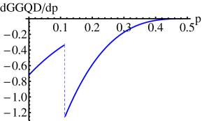
(a) Discontinuous derivative

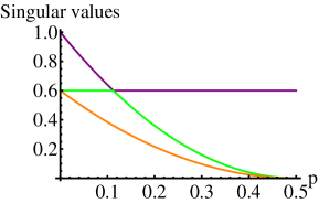
(b) Level crossing

Figure 1: (a) The sudden transition is characterized by a discontinuous change in the time derivative of the discord.  Here this phenomenon is shown for a model in which decoherence comes from phase flips.  p is the probability that a flip has taken place, so p is a monotonically increasing function of time. (b) The transition may be traced back to the a level crossing of singular values f the density matrix.  Here we show the three largest singular values as a function of time.

However, when we have non zero $n_{i3}$, $n_{3i}$ ($i=1,2$) elements, the symmetry is violated and the level crossing goes away.  The singular value evolution is completely smooth and the crossing does not occur.  The contrast between the nearly discontinuous and the smooth behavior is shown in Figure.2.

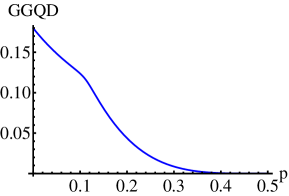
(a) Geometric Global QD

(b) Singular values

Figure 2: (a) The sudden transition is smoothed when the level crossing is avoided.  Here the discord as a function of time shows a smooth crossover from slow to fast decay.   (b) The three largest singular values of the density matrix. The crossing of the two largest singular values is now avoided.  The symmetry that allowed the level crossing in Figure 1(b) has been removed.  

Thus the qualitative conclusion is that the sudden transition is due to a level crossing, which is essentially always a consequence of symmetry; level repulsion due to a small symmetry breaking smooths the crossing, giving rise to a smooth but rapid change, and generic level movement without any symmetry destroys the transition entirely.  Similar conclusions have been reached in [38]. It is important to note that if entropic definitions of discord are used, then rapid changes may still be observed, but the behavior of the discord is always continuous, as pointed out in [39]. This allows us to formulate more quantitatively the conditions for the observation of the sudden transition, for which sudden but not discontinuous change in the slope of geometric global quantum discord is observed, i.e., the level crossing is avoided, but the gap is small. It is motivated by observing that each singular value has contributions from various parts of the generalized Bloch vector, of which only the one from the protected part $n_{33}$ is preserved: $d_{a}=\sum_{ij}n_{ij}R_{ia}^{(1)}R_{ja}^{(2)}=n_{\alpha\alpha}R_{\alpha a}^{(1)}R_{\alpha a}^{(2)}+\sum_{(i,j)\neq(\alpha,\alpha)}n_{ij}R_{ia}^{(1)}R_{ja}^{(2)}$, where $d_{a,robust}\equiv n_{\alpha\alpha}R_{\alpha a}^{(1)}R_{\alpha a}^{(2)}$ is the contribution to $d_{a}$ from the conserved part of Bloch vector. Contributions from other parts vanish as decoherence proceeds (with $p$ approaching $1/2$). Therefore, we model the behavior of each singular value $d_{a}$ to monotonically decrease to $d_{a,robust}$ and the heuristic argument for the sudden transition is that the largest singular value crosses a smaller one as $p$ increases. In this picture, the criteria for the crossing of the largest singular value and the one of the smaller ones is either $|d_{2,robust}(p=0)|>|d_{1,robust}(p=0)|$ or $|d_{3,robust}(p=0)|>|d_{1,robust}(p=0)|$. But this model does not accurately describe the actual behavior, as it does not capture that the $R^{(i)}$s change over time as well and the only one singular value has nonzero value of $n_{33}$ at full decoherence ($p=1/2$). However, if the size of the off-diagonal terms are small enough compared to the other parts, above argument still gives reasonable condition for sudden transition and it converges to the accurate condition as $\epsilon\rightarrow 0$. The previously shown condition of [15] is a special case for $\epsilon\rightarrow 0$ case where $n_{ij}$ is diagonal.

In order to estimate the chance of observing the sudden transition from arbitrary states of the form of Eq.(11), we assume the axis of each rotation $R^{(i)}$ is uniformly distributed over the unit spheres: Pr$(\theta=\theta_{0},\phi=\phi_{0})~{}d\theta~{}d\phi=\frac{1}{4\pi}\sin(\theta_{0})~{}d\theta~{}d\phi$. It corresponds to the random choice of SU(2) unitary matrix according to Haar measure, and we choose the state at random given the three singular values $d_{a},a=1,2,3$. The rotation matrix without nonzero off-diagonal entries corresponds to a rotation in two dimensional space, and the volume of the sets of 2-dimensional rotation matrices in the space of 3-dimentional rotation matrices of course has zero measure. Even if we loosen the condition by allowing a small deviation from the 2-dimensional rotation which results in small probability $\epsilon\ll 1$ for the rotation matrix to have the desired character, the probability of the sudden transition for the 2-qubit system is proportional to $\epsilon^{2}$. For the three or more qubits case where subsystems are maximally mixed ($\rho=\frac{1}{2^{N}}(I+\sum_{a_{1}=1}^{3}\cdots\sum_{a_{N}=1}^{3}n_{\vec{a}}\sigma_{\vec{a}})$) and HOSVD can be applied to the generalized Bloch vector as mentioned earlier ($n_{i_{1}\cdots i_{N}}=\sum_{a}d_{a}\Pi_{k=1}^{N}R_{ai_{k}}^{(k)}$), each rotation matrix $R^{(i)}$ independently gives a additional factor of $\epsilon$ to the chance of the sudden transition so the chance of the transition decays exponentially as $\epsilon^{N}$, as $N,$ the number of qubits, increases.

5 Conclusion

We proposed the use of the generalized Bloch vector for calculation of quantum discord. It makes calculation easier for previously known cases and provides some useful insights on quantum correlation. We showed (under certain weak assumptions) that the calculation of the geometric global quantum discord is an NP-hard problem by considering a certain interesting class of multi-qubit states. It appears to be significantly more difficult to prove corresponding statements for other, non-geometric measures of discord, since they involve more complicated functions.

For states of the form of Eq.(13), we suggested a numerical method to calculate geometric global quantum discord, which appears to be give good results for many interesting models.  When higher-order singular value decomposition is applicable, we proposed a condition to observe the sudden transitions in the geometric global quantum discord, assuming the part preserved by the symmetry of the system and the other parts do not mix significantly. For randomly chosen states, the sharp sudden transition has only a small chance of being observed in the 2-qubit case and it becomes exponentially rarer as the number of qubits increases, because the number of restrictive symmetry conditions needed for this phenomenon to occur increases rapidly with system size.

References

References

• [1] Cleve R and Buhrman H 1997 Phys. Rev. A 56 1201
• [2] Prevedel R, Lu Y, Matthews W, Kaltenbaek R and Resch KΒ J 2011 Phys. Rev. Lett. 106 110505
• [3] Jozsa R and Linden N 2003 R. Soc. London, Ser. A 459 2011
• [4] Vidal G 2003 Phys. Rev. Lett. 91 147902
• [5] Deutsch D and Jozsa R 1992 R. Soc. London, Ser. A 439 553
• [6] Bruß D and Macchiavello C 2011 Phys. Rev. A 83 052313
• [7] Lloyd S 1999 Phys. Rev. A 61 010301
• [8] Meyer D A 2000 Phys. Rev. Lett. 85 2014
• [9] Ollivier H and Zurek W H 2001 Phys. Rev. Lett. 88 017901
• [10] Datta A, Flammia S T and Caves C M 2005 Phys. Rev. A 72 042316
• [11] Datta A, Shaji A and Caves CΒ M 2008 Phys. Rev. Lett. 100 050502
• [12] Passante G, Moussa O and Laflamme R 2012 Phys. Rev. A 85 032325
• [13] Cavalcanti D, Aolita L, Boixo S, Modi K, Piani M and Winter A 2011 Phys. Rev. A 83 032324
• [14] Gu M, Chrzanowski HΒ M, Assad SΒ M, Symul T, Modi K, Ralph TΒ C, Vedral V and Lam PΒ K 2012 Nature Physics 8 671–675
• [15] Maziero J, CΓ¨leri LΒ C, Serra RΒ M and Vedral V 2009 Phys. Rev. A 80 044102
• [16] Mazzola L, Piilo J and Maniscalco S 2010 Phys. Rev. Lett. 104 200401
• [17] Rulli CΒ C and Sarandy MΒ S 2011 Phys. Rev. A 84 042109
• [18] Modi K, Paterek T, Son W, Vedral V and Williamson M 2010 Phys. Rev. Lett. 104 080501
• [19] Luo S and Fu S 2010 Phys. Rev. A 82 034302
• [20] Xu J 2012 Phys. Lett. A 376 320–324
• [21] Xu J 2012 J. Phys. A-Math. Theor. 45 405304
• [22] Girolami D and Adesso G 2011 Phys. Rev. A 83 052108
• [23] Nguyen N and Joynt R 2013 arXiv 1310.5286
• [24] Byrd MΒ S and Khaneja N 2003 Phys. Rev. A 68 062322
• [25] Zhou D and Joynt R 2012 Quantum Inf. Process. 11 571–583
• [26] Luo S 2008 Phys. Rev. A 77 042303
• [27] Ali M, Rau AΒ RΒ P and Alber G 2010 Phys. Rev. A 81 042105
• [28] Lang MΒ D and Caves CΒ M 2010 Phys. Rev. Lett. 105 150501
• [29] Schack R and Caves CΒ M 2000 J. Mod. Optic 47 387–399
• [30] Braunstein SΒ L, Caves CΒ M, Jozsa R, Linden N, Popescu S and Schack R 1999 Phys. Rev. Lett. 83 1054
• [31] Gurvits L and Barnum H 2003 Phys. Rev. A 68 042312
• [32] Bergqvist G and Larsson E 2010 IEEE Signal Proc. Mag. 27 151–154
• [33] DeΒ Lathauwer L, DeΒ Moor B and Vandewalle J 2000 SIAM J. Matrix. Anal. A 21 1253Γ’β‚¬β€œ1278
• [34] Streltsov A, Kampermann H and Bruß D 2011 Phys. Rev. A 84 022323
• [35] Thoft-Christensen P and Murotsu Y 1986 The branch-and-bound method Β Application of Structural Systems Reliability Theory (Berlin, Heidelberg: Springer Berlin Heidelberg) pp 215–265
• [36] Ferraro A, Aolita L, Cavalcanti D, Cucchietti FΒ M and AcΓ¬n A 2010 Phys. Rev. A 81 052318
• [37] Harrow A, Montanaro A 2012 arXiv1001.0017
• [38] Yu C, Li B and Fan H 2013 arXiv1309.0934
• [39] Pinto J, Karpat G and Fanchini F 2013 Phys. Rev. A 88 034304
• [40] Dakic B, Vedral V and Brukner C 2010 Phys. Rev. Lett. 105 190502
• [41] Bellomo B, Giorgi G, Galve F, Franco R, Compagno G and Zambrini R 2012 Phys. Rev. A. 86 012312
• [42] Franco R, Bellomo B, Maniscalco S, and Compagno G 2013 Int. Journ. of Modern Physics B 27 1245053
• [43] Bellomo B, Compagno G, Franco R, Ridolfo A and Savasta S 2011 Journ. of Quant. Inf 9 1665
• [44] Aaronson B, Franco R, and Adesso G 2013 Phys. Rev. A 88 012120
• [45] Huang Y 2014 New J. Phys. 16 033027