Are gamma-ray bursts the same at high redshift and low redshift?

Abstract

The majority of Swift gamma-ray bursts (GRBs) observed at $z\gtrsim 6$ have prompt durations of $T_{90}\lesssim 30$ s, which, at first sight, is surprising given that cosmological time-dilation means this corresponds to $\lesssim 5$ s in their rest frames. We have tested whether the high-redshift GRBs are consistent with being drawn from the same population as those observed at low-redshift by comparing them to an artificially red-shifted sample of 114 $z<4$ bursts. This is accomplished using two methods to produce realistic high-$z$ simulations of light curves based on the observed characteristics of the low-$z$ sample. In Method 1 we use the Swift/BAT data directly, taking the photons detected in the harder bands to predict what would be seen in the softest energy band if the burst were seen at higher-$z$. In Method 2 we fit the light curves with a model, and use that to extrapolate the expected behaviour over the whole BAT energy range at any redshift. Based on the results of Method 2, a K-S test of their durations finds a $\sim$1% probability that the high-z GRB sample is drawn from the same population as the bright low-z sample. Although apparently marginally significant, we must bear in mind that this test was partially a posteriori, since the rest-frame short durations of several high-z bursts motivated the study in the first instance.

1 Introduction

Gamma–ray bursts (GRBs) are identified as short-lived (seconds to minutes in most cases) transient flashes of gamma-rays (Klebesadel et al., 1973). Their light curves show great diversity in behaviour, ranging from the very smooth to the highly erratic (Paciesas et al., 2012; Sakamoto et al., 2011, 2008; Paciesas et al., 1999). Much effort has been expended over the decades in trying to classify and understand this diversity (Bromberg et al., 2013; Kann et al., 2011; Zhang et al., 2007; Norris & Bonnell, 2006; Gehrels et al., 2006; Reichart et al., 2001; Norris et al., 2000; Kouveliotou et al., 1993), although arguably the most useful observables remain the comparatively gross properties of duration and average spectral hardness. In particular, these properties serve to separate out the two classical sub-classes of GRB, namely the long-duration/soft-spectrum and the short-duration/hard-spectrum (Bromberg et al., 2013; Kouveliotou et al., 1993).

An important question is whether the populations of GRBs change with redshift, which in principle might be reflected in the typical prompt behaviour. In fact, it does seem that the short-GRBs (Nakar, 2007) are on average fainter and visible at lower redshifts than the long-GRBs. Beyond this, the only tentative evidence for an evolution in the population of long-GRBs is that several of the highest redshift GRBs found to-date have apparently rather short durations, $T_{90}\lesssim 5$ s, in their rest frames (Gorbovskoy et al., 2012; Cucchiara et al., 2011a; Tanvir et al., 2009; Greiner et al., 2009). Several works have argued that these are most likely not misclassified short-bursts (e.g., Lü et al., 2012; Zhang et al., 2009; Belczynski et al., 2010), so it is natural to ask whether their unusual properties could be indicating some change in the typical long-GRB progenitors, possibly due to their having very low metallicity. The difficulty in assessing the significance of this finding is firstly that samples remain rather small, and secondly that measured duration is actually dependent on detector sensitivity and band-pass, in addition to the underlying behaviour of the given GRB and indeed the chosen operational definition of “duration”. Hence even when using the same instrument, inferring rest-frame duration by simply dividing the observed duration by the cosmological time-dilation factor may well produce misleading results.

In a previous study Kocevski & Petrosian (2013) simulated GRBs as they would be observed by the Burst and Transient Source Experiment (BATSE; Meegan et al. 1992) instrument, to find whether signatures of time dilation might be detected in properties such as $T_{90}$ (see §2). In that work the authors used prescriptions for the shape and time evolution of GRB spectra to produce single-pulse prompt high-energy light curves. These simulations showed that cosmological time dilation is often not reflected in the measured duration of a burst. In some instances the duration of a synthetic burst could be seen to decrease as a function of the simulated redshift, particularly when the signal to noise ratio became poor. A limitation of the work presented in Kocevski & Petrosian (2013) is that the simulated light curves all contained only a single morphological feature: one Fast Rise Exponential Decay (FRED) pulse. The authors suggested that time dilation might be more apparent in GRB temporal profiles that contained narrow pulses separated by periods of quiescence. In such a situation, it would be the increasing duration between peaks that would provide the signature of this time dilation.

In this paper we seek to make a more robust comparison of observed low- and high-redshift GRB populations, by taking a large sample of the former and artificially “redshifting” them to see how they would appear if they had occurred at high-$z$. This procedure is amenable to simulation since signal-to-noise tends to reduce with increasing redshift, largely masking uncertainties introduced in the band-shifting. We develop two methods of simulation, which are presented in § 4, along with our recipe to emulate the Swift Burst Alert Telescope (BAT; Barthelmy et al. 2005) “rate triggering” (only) algorithm, and descriptions of the various duration measures we consider. In § 5 we study in detail the evolution of 16 bright bursts with simulated redshift. Finally in § 6 we analyse the simulated prompt light curves of 114 ($z<4$) GRBs and compare the detectable fraction to the currently known high-redshift Swift bursts, assessing whether they are consistent with being drawn from the same parent population.

2 Measures of duration

2.1 $T_{90}$

The durations of the high–energy prompt emission of GRBs are commonly parameterised by $T_{90}$ which is defined as the time between which 5% and 95% of the total fluence received in the observer-frame is measured (similarly $T_{50}$, for example, is the time between which 25% and 75% of the total fluence is received). In Figure 1 we plot the $T_{90}\left(15-350~{}{\rm keV}\right)$ distribution as a function of redshift for the 203 GRBs detected by Swift (Gehrels et al., 2004) since launch that were seen prior to the 2012 July 15^th and have a measured redshift (either from emission lines, absorption lines or a photometric redshift). We use the values for $T_{90}$ available from the Swift ground analysis, which are obtained by running the Bayesian blocks algorithm battblocks as part of the batgrbproducts script. battblocks is run on light curves of several different bin sizes (4 ms, 16 ms, 1 s and 16 s), before applying a set of criteria to determine the best $T_{90}$ duration estimate (Sakamoto et al., 2011).

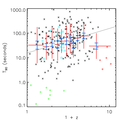
Figure 1: The observed distribution of $T_{90}$ for the 203 Swift bursts with a redshift estimate prior to 2012 July 15^th (note this includes a mixture of redshifts determined directly from afterglows and those inferred via host galaxy spectroscopy). Also included are GRB 120521C and GRB 120923A which both are candidates for high-redshift. The red crosses show geometric averages of bursts taken with 20 bursts in each bin (except in the final bin which has 16 bursts). The red error bars shown in the vertical direction show the root mean square (RMS) scatter calculated logarithmically. Also shown are the standard errors on the mean for each bin in blue. The dotted black line shows the expected evolution due to simple cosmological time dilation, namely $T_{90}\propto 1+z$. Short GRBs are denoted by the green diamonds. The high-redshift subset of six GRBs shown in Figure 13 are indicated by red diamonds. The low-redshift, bright subset introduced in §3.1 are denoted by blue squares. Redshift were obtained from http://swift.gsfc.nasa.gov/docs/swift/archive/grb_table/.

The calculated means do not include short GRBs, as these tend to be observed in the more local Universe. As such they reduce the averages of the lowest redshift bins in a manner that could be mistaken for time dilation.

Whilst the geometric RMS scatter in Figure 1 is large, it is interesting that the mean values can be seen to increase slightly over almost the entire redshift range of the observed population, broadly in line with the expected effect of cosmological time dilation i.e., $T_{90}\propto 1+z$. The standard-errors on these means are shown as shorter error bars, suggesting that the trend is no more than moderately significant, and, indeed, that a no-evolution model cannot be ruled out. To test this we fitted two models: one with no evolution, finding $T_{90}=45.8\pm 5.4$ seconds, and another where $T_{90}\propto 1+z$ ($T_{90}=11.7\pm 1.6\left(1+z\right)$ seconds). For the no-evolution model we obtained a $\chi^{2}=10.39$, for 10 degrees of freedom ($\chi^{2}_{\nu}=1.04$), whilst the $T_{90}\propto 1+z$ model had a $\chi^{2}=5.93$ for 9 degrees of freedom (reduced $\chi^{2}$=0.66). Of the two, the $T_{90}\propto 1+z$ has the lower $\chi^{2}_{\nu}$ fit statistic, by $\Delta\chi^{2}_{\nu}=0.38$. Only for the final bin, containing the highest redshift bursts with $4.65$ $\leqslant$ $z$ $\leqslant$ $9.4$, does the geometric mean $T_{90}$ fall significantly below either trend.

Shown in Figure 2 are the distributions all Swift burst $T_{90}$ values when divided according to whether a redshift was measured for each. As can be seen, the two distributions agree with one another to a reasonable extent. To test this we performed a Kolmogorov-Smirnov (K-S) test on the two samples. This statistical test compared the cumulative distributions of two data sets to find whether the two arise from a common parent population. From the K-S test, we derived a probability of $p=0.1$, which is large enough that the two samples cannot be distinguished with any statistical significance. This implies that the two populations shown in Figure 2 are not markedly different and that no duration bias is introduced by only considering bursts with available redshifts.

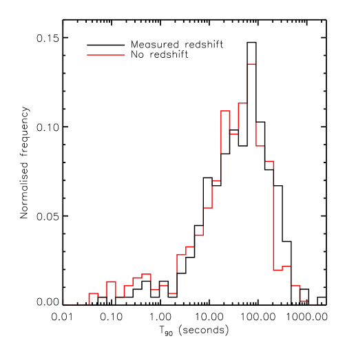
Figure 2: $T_{90}$ distributions for Swift bursts with and without redshifts. The black line corresponds to bursts with a measured redshift, whilst the red distribution is for those bursts which don’t. The total population extends from the launch of Swift, including 224 bursts with a redshift and 459 without one.

2.2 An alternative measure of duration

In an attempt to diminish the effect of background noise we also adopted an alternative measure of prompt duration. From a dynamic binning routine that bins the 64 ms light curves to a minimum significance threshold, we found the brightest bin in the re-binned light curve. We used this value to define a brightness threshold of half of this maximum flux ($F_{\rm thresh}$ $=$ 0.5$F_{\rm max}$). We summed the duration of all bins which were above this threshold. This was termed the “core time” $T_{\rm c}$, and measures the period of time over which the source can be considered to be most active. Measures such as $T_{90}$, which are defined over contiguous bins, may include quiescent periods between regions of activity, whereas $T_{\rm c}$ will remain insensitive to such times. A plot of $T_{\rm c}$ versus redshift is shown in Figure 3, and again demonstrates a weak trend of increasing duration with redshift, up to $z\sim 5$. A similar measure has previously been used in works such as Reichart et al. (2001): specifically they considered the duration of the brightest bins in the light curve that accounted for 50% of the observed fluence.

As for $T_{90}$, we fitted both a no-evolution model ($T_{c}=5.23\pm 0.38$ seconds) and one which was proportional to $1+z$ ($T_{c}=1.30\pm 0.11(1+z)$ seconds), as expected from cosmological time dilation. For the no-evolution model, we found $\chi^{2}=30.26$, with 9 degrees of freedom ($\chi^{2}_{\nu}=3.36$), whilst the $T_{c}\propto\left(1+z\right)$ model had $\chi^{2}=26.25$ for 8 degrees of freedom ($\chi^{2}_{\nu}=3.28$). In terms of $\chi^{2}_{\nu}$, the $T_{c}\propto\left(1+z\right)$ proved a better fit with $\Delta\chi^{2}_{\nu}=0.08$, although this improvement is marginal due to the nature of the data. The $T_{c}\propto\left(1+z\right)$ model is the dotted line plotted in Figure 3.

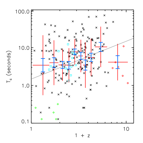
Figure 3: The observed distribution of $T_{\rm c}$ versus redshift. The high-redshift burst sample are shown by red diamonds, whilst the low redshift sample are shown by blue squares. Short bursts ($T_{90}<0.8$ seconds) are denoted by green diamonds. The dashed line shows the $T\propto 1+z$ expected from simple cosmological time dilation. As with $T_{90}$ (Figure 1) the binned averages show a weak trend of increasing duration with redshift up to $z\sim 5$.

3 Data

As a basis for our simulations of high-redshift bursts, we considered GRBs observed by Swift prior to 2011 May 3^rd for which redshifts have been reported.

3.1 Selection of low-redshift bursts

This work aims specifically to predict the morphology of the prompt high-energy light curves, and key parameters such as $T_{90}$, of high-redshift GRBs based on the properties of those at low-redshift. To maximise the baseline in redshift, we considered only the 175 Swift bursts prior to 2011 May 3^rd with observed redshift, $z_{\rm orig}$ $<$ 4. Of these, we retained those fitted with the Willingale et al. (2010) pulse model (essentially these were all Swift GRBs observed before 2011 May 3^rd, for which the satellite was able to execute a prompt slew and hence gather early X-ray data; see also §3.3). This yielded 114 GRBs which were simulated at high-redshift, as detailed in §6.

To also effect a detailed case study of the evolution of measured durations with increased simulated redshift, we identified a smaller sample of bursts, bright enough to have a realistic possibility that they would have been detected (see also § 4.3) had they occurred at $z\sim 6$. We identified these as having at least one pulse with a peak bolometric luminosity $L_{\rm pk}$ $>$ $1.0\times 10^{52}{\rm{\rm\thinspace erg}{\rm\thinspace s}^{-1}}$. This value was chosen to ensure that we simulated all bursts that produced detectable structure using both simulation methods at $z_{{\rm sim}}\sim 6$, but to also avoid the simulations of a larger sample of bursts that would not be detected at high-redshifts.

This peak luminosity made use of the model fits described in § 4.2, and was calculated using Equation 1, where $D_{L,orig}$ is the luminosity distance to the burst as observed, $S_{pk}$ is the brightest pulse normalisation across the BAT band as defined in Willingale et al. (2010) and $K_{\rm orig}$ is the $K$-correction required to convert this 15 – 350 keV fluence normalisation to a bolometric fluence.

$$L_{\rm pk}=4\pi D_{\rm L,orig}^{2}K_{\rm orig}S_{\rm pk}.$$ (1)

This selection produced 16 bursts, some with multiple pulses that satisfied the luminosity threshold. These GRBs and the properties of their brightest pulses are detailed in Table 1. It is important to emphasise that since we are dealing with just the brightest $z_{{\rm orig}}<2$ GRBs it is unlikely that any selection effects, such as the requirement for a redshift determination, will introduce any bias in the distribution of durations.

Table 1: The bright GRB subset identified for our detailed morphological case study. Values of $T_{90}$ are those obtained from the standard BAT analysis. $N_{p}$ denotes the number of modelled pulses used for fitting the light curves, $b_{1}$, $S_{pk}$ and $L_{pk}$ all correspond to the relevant values of the brightest pulse in each burst. (Redshifts obtained from: 1. Foley et al. (2005), 2. Vreeswijk et al. (2007), 3. Fynbo et al. (2009), 4. Page et al. (2007), 5. Racusin et al. (2008), 6. Wiersema et al. (2008), 7. Krühler et al. (2012), 8. Gendre et al. (2010), 9. Chornock et al. (2009), 10. McBreen et al. (2010), 11. Xu et al. (2009), 12. O’Meara et al. (2010), 13. Gorbovskoy et al. (2012), 14. Cucchiara et al. (2011b), 15. de Ugarte Postigo et al. (2011) and 16. D’Avanzo et al. (2011))

GRB	Redshift	$T_{90}(z_{\rm orig})$	$N_{\rm p}$	$b_{1}$	$S_{\rm pk}$	$L_{pk}$
		(s)			(keV cm${}^{{\rm-2}}\,{\rm s}^{-1}$)	(${\rm{\rm\thinspace erg}{\rm\thinspace s}^{-1}}$)
GRB 050525A	0.6061	8.86 $\pm 0.07$	7	0.06	4441.78	1.08 $\times$ 1052
GRB 060418	1.4892	109.17 $\pm 46.73$	9	-0.38	576.42	1.32 $\times$ 1052
GRB 060908	1.8843	18.78 $\pm 1.30$	4	0.11	256.88	1.05 $\times$ 1052
GRB 061121	1.3144	81.22 $\pm 46.40$	7	0.48	2619.25	4.39 $\times$ 1052
GRB 080319B	0.9375	124.86 $\pm 3.10$	17	1.11	2757.78	1.98 $\times$ 1052
GRB 080319C	1.9506	29.55$\pm 9.41$	3	0.01	538.89	2.40 $\times$ 1052
GRB 080605	1.6407	29.55 $\pm 9.41$	9	0.29	2622.20	7.63 $\times$ 1052
GRB 090102	1.5478	29.30 $\pm 3.23$	3	0.20	512.07	1.29 $\times$ 1052
GRB 090424	0.5449	49.47 $\pm 2.27$	6	0.12	5744.63	1.08 $\times$ 1052
GRB 090510	0.90310	5.66 $\pm 1.88$	1	0.52	1761.86	1.16 $\times$ 1052
GRB 091020	1.71011	38.92 $\pm 4.89$	4	-0.24	354.11	1.14 $\times$ 1052
GRB 100814A	1.44012	174.72 $\pm 9.47$	17	0.57	482.72	1.01 $\times$ 1052
GRB 100906A	1.72713	114.34 $\pm 1.59$	14	0.00	636.66	2.10 $\times$ 1052
GRB 110213A	1.46014	48.00 $\pm 16.00$	6	-0.95	498.70	1.08 $\times$ 1052
GRB 110422A	1.77015	25.77 $\pm 0.60$	7	0.03	2167.60	7.60 $\times$ 1052
GRB 110503A	1.61316	10.05 $\pm 3.41$	1	-0.05	2799.08	7.81 $\times$ 1052

3.2 BAT data

BAT data are used in both simulation methods detailed in §4. The data, including auxiliary data and the Tracking and Delay Relay Satellite System (TDRSS) data, were downloaded from the UK Swift Science Data Centre (UKSSDC; http://www.swift.ac.uk/swift_portal/). These raw data were processed using the standard Swift routine batgrbproduct.

One of the resulting outputs of batgrbproduct is a series of GRB light curves taken at multiple temporal resolutions in either one total (15–350 keV) band or the four individual bands (15–25 keV, 25–50 keV, 50–100 keV and 100–350 keV) as used in typical BAT analysis. The observed BAT light curves for the bright ($z_{{\rm orig}}<2$) sample are shown in Figure 4, where the light curves shown are those obtained when the four bands are summed for each burst.

Figure 4: High-energy 15–350 keV BAT light curves of the low redshift bright burst sample. The light curves are binned at 256 ms to allow clear identification of structure within each. There is also a dashed line in each panel to show a zero count rate.

3.3 XRT data

Swift X-Ray Telescope (XRT; Burrows et al. 2005) data have not been simulated in this work, however, as discussed in §4.2 below, the second method used to simulate BAT light curves does involve modelling of both BAT and XRT data following the method of Willingale et al. (2010). Therefore an additional criterion for inclusion in the sample is that Swift executed a prompt slew to the burst, thus providing the necessary early-time X-ray observations, although we emphasise that there is no requirement that the X-ray data overlap the period of activity detected by BAT. The speed at which Swift slews its narrow–field instruments to a new GRB is determined solely by observing constraints; including, for example, the proximity of the source to the Sun or Moon, or whether such a source is occulted by the Earth. Thus this selection criterion does not bias our sample.

4 Modelling

Two different methods of simulation were developed. The first uses the observed BAT data in the spectral range that would fall within the 15–25 keV band if the burst in question had occur at the simulated higher redshift ($z_{{\rm sim}}$). The second method uses the prompt pulse model detailed in Willingale et al. (2010), as fitted to the observed BAT and XRT data, evolving the characteristic times, energies and normalizing fluxes that describe each pulse. We describe each in the following sections (with further details in the appendices).

In both cases, creation of the simulated light curves required accounting for the effects of cosmological time dilation; of band-shifting, as individual photons are redshifted (this included consideration of the BAT response and changes in background as a function of energy); and of declining flux due to increased luminosity distance as defined in Equation 2.

$$F(E_{1}\mapsto E_{2})=\frac{L(E_{1}(1+z)\mapsto E_{2}(1+z))}{4\pi(D_{L}(z))^{2}}.$$ (2)

Here $F(E_{1}\mapsto E_{2})$ is the flux of the bin in a specified observing band between photon energies $E_{1}$ and $E_{2}$, $L(E_{1}(1+z)\mapsto E_{2}(1+z))$ is the corresponding luminosity in the same de-redshifted band and $D_{L}(z)$ is the luminosity distance of the source at redshift $z$. To calculate luminosity distances we adopted a standard $\Lambda CDM$ cosmology with $H_{0}$ = 71 km s^-1 Mpc^-1, $\Omega_{m}$ $=$ $0.27$ and $\Omega_{\Lambda}$ $=$ 0.73.

4.1 Method 1: High-redshift simulations made directly from BAT data

In our first method (Method 1 hereafter) we aimed to produce a simulated 15–25 keV observer-frame light curve for a GRB located at $z_{\rm sim}$. To do so, we extracted a light curve from the observed BAT data for a burst at $z_{\rm orig}$ at 64 ms resolution using the standard batbinevt routine, which also subtracts the background. Specifically, we produced the light curve in the 15${F_{\rm z}}$–25${F_{\rm z}}$  keV range, where for convenience we have defined ${F_{\rm z}}$ as shown in Equation 3.

$${F_{\rm z}}=\frac{1+z_{\rm sim}}{1+z_{\rm orig}}.$$ (3)

So, in an instance where $z_{{\rm orig}}=1$ and $z_{{\rm sim}}=3$, ${F_{\rm z}}=2$ and we were required to use batbinevt to extract both a 15–25 keV and 30–50 keV light curve.

Figure 5: The BAT effective area per detector as a function of energy. The vertical dotted lines show the energy ranges of the four standard BAT channels as described is §3.2.

We needed to account for the energy dependence of the BAT sensitivity, $A(E)$, which is shown in Figure 5. As can be seen, for higher energies the integrated effective area is small. For simplicity we assumed that the effective area of the detector over the energy band of interest could be taken simply as an average of $A(E)$ over that band (strictly speaking one should weight by the spectral energy distribution of the source, but this will usually not be a large correction, and we neglect it at this stage so as to avoid introducing any model fitting). Hence, for each bin in the original light curve, defined by start and end times $T_{1}$ and $T_{2}$, we can relate the photon counts in the simulation to the original counts via:

$$\begin{array}[]{lll}C_{\rm sim}(T_{1}{F_{\rm z}}\mapsto T_{2}{F_{\rm z}})&=&{F_{\rm z}}^{2}\left(\frac{D_{\rm L,orig}}{D_{\rm L,sim}}\right)^{2}\frac{\int\limits_{15}^{25}A\left(E\right).dE}{\int\limits_{15{F_{\rm z}}}^{25{F_{\rm z}}}A\left(E\right).dE}\\ &&\times C_{\rm orig}(T_{1}\mapsto T_{2}),\\ &=&QC_{\rm orig}(T_{1}\mapsto T_{2}).\end{array}$$ (4)

Thus the quantity $Q$ provides the factor by which the observed counts in the 15${F_{\rm z}}$–25${F_{\rm z}}$ light curve at $z_{\rm orig}$ must be reduced to calculate the 15–25 keV light curve at $z_{\rm sim}$. $Q$ is dependent on three contributions: the change in luminosity distance, the redshifting of the photons and the change in sensitivity of the BAT instrument between the two energy bands. Providing $Q<1$, we can therefore produce a new simulated light curve with the right noise characteristics by simply losing an appropriate number of the original counts from each bin, prior to rebinning back to an observed 64 ms time resolution.

Finally, we ensured that the background noise was adjusted to match that expected in the 15–25 keV band, as measured in the original data. These steps are described in more detail in Appendix A.

4.2 Method 2: Simulations using the prompt pulse model

The disadvantage in using the BAT data directly, as we did in Method 1, is the restriction imposed by the finite energy response. Consequently, we required that 25${F_{\rm z}}$ $<$ 350 keV for the simulation to be within the BAT coverage. Aside from this, the uncertainties due to the shape of the BAT spectral response increase significantly at the upper end of this energy range, reducing confidence in the simulations conducted at the highest redshifts. In practice, then, we are limited to ${F_{\rm z}}\lesssim 10$.

An alternative and more flexible approach is to fit models to the temporal and spectral behaviour of the real GRBs, and use these models as the basis for simulations. Specifically, we followed Willingale et al. (2010) who fit both the observed BAT and XRT light curves simultaneously using a combination of the pulse model of Genet & Granot (2009), first proposed to explain the steep decay phase (SDP) as a result of high latitude emission, and a phenomenological afterglow model (Willingale et al., 2007). The Genet & Granot (2009) model includes spectral evolution, and so being able to fit the SDP, which is not seen in the BAT light curves, helps constrain the decay of all pulses. This is the reason that availability of early-time XRT data was one of the criteria used to select our sample (see §3.3).

Using this methodology (Method 2 hereafter) we calculated the flux light curves of all four primary BAT and the two XRT channels (the BAT channels being as described in §3.2 and the XRT channels being 0.3–15 keV and 1.5–10 keV), allowing a more extensive analysis of the high-energy characteristics of the prompt emission. To conduct such simulations the parameters of each prompt pulse, and also the X-ray afterglow, needed to be evolved to the values that would be observed by placing the burst progenitor at a higher redshift. Figure 1 of Willingale et al. (2010), which is a representation of a single pulse temporal profile, shows the characteristic times associated with each pulse. These include the time over which a pulse rises ($T_{\rm r}$), the time at which the pulse peaks ($T_{\rm pk}$) and the arrival times of the first and last photons ($T_{0}$ and $T_{\rm f}$). The values of these at the simulated redshift were calculated using time dilation as shown in Equation 5, where $T_{\rm sim}$ and $T_{\rm orig}$ correspond to any of the characteristic timescales at the simulated and observed redshifts respectively.

$$T_{\rm sim}={F_{\rm z}}\times T_{\rm orig}.$$ (5)

In this model, the spectrum of each of the pulses is a time evolving exponentially cut–off power-law. The peak energy of the $\nu F_{\nu}$ spectrum is defined at the time when the pulse peaks in the light curve of the GRB, $T_{\rm pk}$. When a pulse is simulated at a higher redshift, time dilation causes $T_{\rm pk}$ to occur later. Furthermore, the photon energy at the peak of the spectrum, $E_{\rm pk,sim}$, reduces as a pulse is placed at a higher luminosity distance.

$$E_{\rm pk,sim}=\frac{E_{\rm pk,orig}}{{F_{\rm z}}}.$$ (6)

Finally, each pulse has a normalizing flux, $S_{\rm pk,sim}$, which was calculated from the original normalisation, $S_{\rm pk,orig}$, using Equation 7.

$$S_{\rm pk,sim}=\left(\frac{K_{\rm orig}}{K_{\rm sim}}\right)\left(\frac{D_{\rm L,orig}}{D_{\rm L,sim}}\right)^{2}S_{\rm pk,orig}.$$ (7)

As previously discussed, the k–correction, $K$, is used to convert the fluence in either the observed or simulated energy band to the bolometric fluence of the pulse.

Once the pulse parameters were adjusted, we ran the models through the same software used to produce light curves such as those shown in Willingale et al. (2010). This provided smooth 64 ms light curves that were background subtracted in each of the four BAT bands. These model light curves formally contain no statistical noise from either the source or the background, so finally we added artificial scatter to account for both, as elaborated in Appendix B.

4.3 Rate triggering algorithm

To provide a fair comparison to the observed high-redshift GRBs it is essential to establish whether or not a given simulated light curve would actually have triggered Swift/BAT. This requires an algorithm that emulates the BAT trigger process. In practice, that is very hard to do fully realistically, so we restrict ourselves to only considering “rate” triggers.

For each rate-trigger we considered two durations measured by BAT: a trigger and background duration. Of those background regions measured by BAT, we took that which occurs prior to the region of the light curve during which the burst is active. The trigger duration is a narrower window that constantly runs through the on-board BAT data. The total fluence within this window is cumulated and if the signal to noise ratio of the total fluence exceeds a predefined threshold, the algorithm reports a trigger to begin normal Swift GRB observations.

To define the trigger durations used in our algorithm, we considered all Swift bursts which triggered BAT. For each burst we looked at the durations of the trigger and the background, as well as the energy ranges used to find the standard combinations for typical BAT triggers. These real combinations of trigger and background durations are shown in Figure 6.

Figure 6: Background duration as a function of trigger duration used in the BAT detection algorithm for all bursts that triggered the Swift/BAT (excluding GRB 041228, as discussed).

The BAT algorithm has a well defined set of combinations of background and trigger durations. We exclude GRB 041228 (with a trigger duration of 64 ms and a background duration of 40 seconds) due to having an unusual trigger, not successfully used in any subsequent burst. The majority of bursts trigger on a 1024 ms trigger and 8 second background duration, in the 25 – 100 keV range. This corresponds to channels 2 and 3 of BAT.

We selected a background region that occurred before the trigger time, which was chosen to maximise the total fluence within the trigger duration. Using these regions, we applied Equation 8, taken from Fenimore et al. (2003), to calculate the trigger significance.

$$S=\frac{\left(C_{j}-2^{j-10}B\right)^{2}}{2^{j-10}B+\sigma_{min}^{2}}.$$ (8)

In Equation 8, $C_{j}$ is the total number of counts in the region of the light curve containing the most counts, whilst $B$ is the number of background counts expected in 1024 ms. $j$ is defined by the binning of the light curve, with each bin being $2^{j}$ ms in duration. In effect, the numerator of Equation 8 is the background corrected number of counts within the trigger duration. $\sigma_{min}$ ensures there is always a minimum value of variance. However, as we specified a realistic, non-negligible background, we did not include $\sigma_{min}$ when calculating $S$. It was $S$ that we used to judge whether the detectability of a given light curve using BAT.

Only the combinations shown in Figure 6 (discounting that for GRB 041228) were used to define background and trigger times. Additionally, to further mimic Swift and also minimise processing time, the triggers were ordered by how often they had occurred within the real burst population. Once a trigger was successfully satisfied at 6.4$\sigma$ the algorithm stopped checking further triggers.

It is important to note that our rate-triggering algorithm is conservative, in the sense that, while it may designate some simulations “undetected” when the real BAT would have triggered on them (since the Swift in-flight software includes more elaborate criteria, such as image triggers), it is unlikely that any light curves we claim are “detected” would have been missed by BAT. Thus our simulations should provide a fair comparison to the Swift high-$z$ sample, which all would have triggered BAT based upon this algorithm.

4.4 Measuring $T_{90}$

The simulated light curves produced files in the standard template used by the routine battblocks for calculating $T_{90}$. battblocks uses a Bayesian analysis to find robust duration measures (Scargle, 1998) including the time intervals $T_{90}$, $T_{50}$ and, if required, any duration specified by the user.

Aside from modifying the values of flux, time and error, key parameters within the data files, such as the start, stop and exposure times of the significant proportions of the light curve had to be altered. These were adjusted using the temporal factor shown in Equation 5.

We ran battblocks at a temporal resolution of 1024 ms. Binning the simulated light curves at such a resolution, rather than directly from the 64 ms output, proved useful, as when the signal became weak, the coarser temporal binning allowed for more reliable calculation of $T_{90}$.

5 A detailed case study of 16 bright bursts

Taking the 16 bursts identified with bright pulses, we simulated each at a variety of redshifts in the range 2 $\leqslant$ $z$ $\leqslant$ 12. The simulations were conducted at small increments in redshift of $\Delta z$ $=$ $0.125$ up to $z$ $=$ 5, and in steps of $\Delta z$ $=$ $0.5$ thereafter.

Both simulation methods used these values for $z_{\rm sim}$, however, Method 1 was restricted in some cases due to the limited spectral coverage from BAT. In these cases the simulations could not be performed past ${F_{\rm z}}$ $=$ 6. This affected four of the bright bursts: GRB 050525A, GRB 080319B, GRB 090424 and GRB 090510, although in all cases the triggering algorithm failed to detect structure prior to the cut off in the simulations.

In practice, at higher redshifts the measured durations become very uncertain, so for each burst we ran 100 simulations at each redshift. The measured durations (where the burst still satisfied the trigger criteria) were then averaged, using the geometric mean.

5.1 Results of Method 1

Using Method 1 to simulate the 15–25 keV light curves of the bright subset revealed that only six bursts would be detected in at least 90% of the simulations at $z_{\rm sim}$ $=$ 6. Example light curves at this simulated redshift are shown in Figure 7.

Figure 7: 15–25 keV BAT light curves of the bright burst subset when simulated at $z_{\rm sim}$ $=$ 6 using Method 1. The light curves are binned at 1024 ms to allow clearer identification of structure within each. Only those bursts which were detected using the BAT algorithm at $z_{\rm sim}$ $=$ 6 are shown. There is also a dashed line in each panel to show a zero count rate.

The standard battblocks algorithm was run on all simulated light curves. The BAT triggering algorithm was then used to identify which of the light curves contained detectable structure in the 15–25 keV range. The geometric average of the triggered light curves was then taken at each $z_{\rm sim}$ for each burst. These are shown in the left panels of Figure 8, which also shows the measured $T_{90}$ for the observed high-redshift bursts.

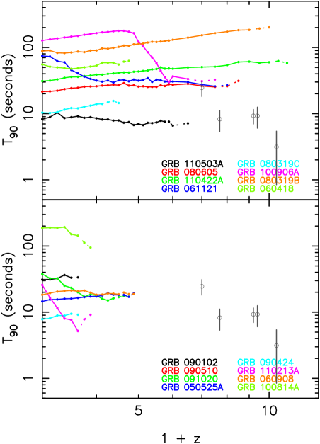
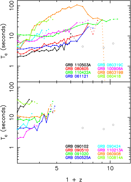
Figure 8: Predictions of observed durations using Method 1 ($T_{90}$ and $T_{c}$ on the left and right, respectively) of bright bursts as they would have been seen if they had occurred at higher redshift. Each coloured line corresponds to simulations of a single GRB in the bright sample, with each duration being averaged over 100 repeated simulations. The sample has been split according to the luminosity of the brightest pulse in each burst (see Table 1), with the most luminous 8 being shown in the top panel. Solid lines show where the burst was detected in a minimum 90% of the repeated simulations, the dotted lines show where the burst was detected in less than 90% but greater than 50% of these repeats. The grey open circles correspond to the 15–25 keV $T_{90}$ and $T_{c}$ values of the observed high-redshift bursts in the left and right panels respectively.

In Figures 8 and 10 the simulated bursts have been divided into two subsets based on their peak luminosities to make it easier to see the evolution of each. The eight bursts with the brightest peak luminosities are in the top panel, with the remaining eight shown in the bottom panel.

The same process was repeated for $T_{c}$. The results of this are shown in the right panels of Figure 8. Once more the same analysis has been conducted on the observed 15–25 keV light curves of the high-redshift sample for reference. Only three of the six bursts were bright enough to define a bright core exclusively in the 15–25 keV range.

5.2 Results of Method 2

Using Method 2 there were 12 bursts in the bright sample that were detected when simulated at $z_{\rm sim}$ $=$ 6. Examples of the 15–350 keV light curves produced for these bursts are shown in Figure 9, where the light curves are binned at 1024 ms to make the presence of structure easier to discern by eye.

Figure 9: 15–350 keV BAT light curves of the bright burst subset when simulated at $z_{\rm sim}$ $=$ 6 using Method 2. The light curves are binned at 1024 ms to allow clearer identification of structure within each. Only those bursts which were detected using the BAT algorithm at $z_{\rm sim}$ $=$ 6 are shown. There is also a dashed line in each panel to show a zero count rate.

We also plotted the evolution of $T_{90}$ with redshift for all the bright bursts. This is shown in the left panels of Figure 10, where the four channel 15–350 keV simulations obtained using Method 2 were summed to create a single channel. This 15 -350 keV light curve was analysed using battblocks in an identical manner to both Method 1 and the regular Swift/BAT analysis. Once more the observed $T_{90}$ values of the high-redshift sample are also shown in the left panels of Figure 10.

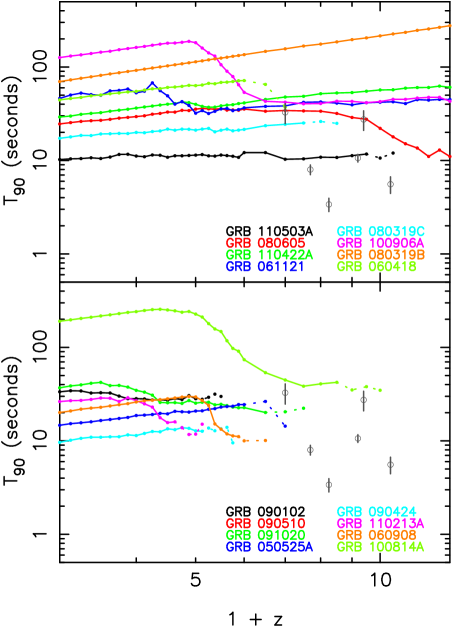
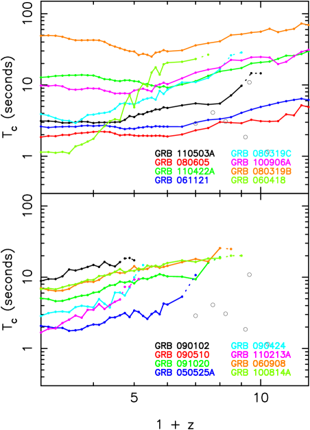
Figure 10: Predictions of observed durations using Method 2 ($T_{90}$ and $T_{c}$ on the left and right, respectively) of bright bursts as they would have been seen if they had occurred at higher redshift. Each coloured line corresponds to simulations of a single GRB in the bright sample, with each duration being averaged over 100 repeated simulations. The sample has been split according to the luminosity of the brightest pulse in each burst (see Table 1), with the most luminous 8 being shown in the top panel. Solid lines show where the burst was detected in a minimum 90% of the repeated simulations, the dotted lines show where the burst was detected in less than 90% but greater than 50% of these repeats. The grey open circles correspond to the 15–350 keV $T_{90}$ and $T_{c}$ values of the observed high-redshift bursts in the left and right panels respectively..

We derived $T_{c}$ for all the simulated light curves produced using Method 2. The averages of the light curves with structure that would trigger BAT are shown in the right panels of Figure 10. Method 2 allowed us to find $T_{c}$ over the entire 15–350 keV range. All six of the observed high-redshift sample were bright enough to define a bright core across this spectral range.

5.3 Evolution of $T_{90}$

The behaviour of each burst in the left-hand panels of Figures 8 and 10 can be reasonably well understood by considering the effects of cosmological time dilation leading to an increase in duration (seen most clearly for GRB 080319B), together with the opposing tendency for declining signal-to-noise and band-shifting to reduced duration. The latter effects depend on the morphology of the light curve: in particular the fact that GRB prompt emission often shows hard-to-soft evolution means that later peaks are likely to become undetected before earlier peaks resulting in the conspicuous decline in observed duration seen in some cases (e.g., GRB 100906A beyond $z_{\rm sim}$ $=$ 5; see also Figure 11). In some cases, such as GRB 110503A and GRB 080319C, the duration is almost independent of redshift, due to the loss of detected flux in the wings of the prompt emission approximately cancelling out the effects of time dilation.

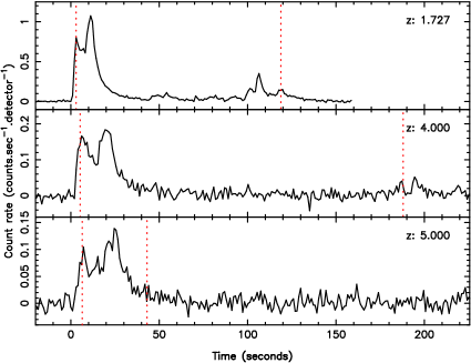
Figure 11: 15 – 350 keV light curve simulations of GRB 100906A at three redshifts. From top to bottom these redshifts are $z$ $=$ 1.727, 4, and 5. $z$ $=$ 1.727 is the observed redshift of the burst. The binning of this light curve is 1024 ms and the red dotted lines show the start and end of the identified $T_{90}$ period. Note that the vertical scaling is different in the three panels. The figure illustrates how the observed duration can decrease rapidly with redshift when some phase of the emission, in this case the second major peak, drops below detectability.

As can be seen in Figure 11, as $z_{\rm sim}$ increases the signal to noise ratio of structure within the light curve significantly reduces. As such, it is expected that the uncertainty in the average values obtained for $T_{90}$ at high-redshift will be high. These uncertainties have not been included on Figures 8 and 10 as it was felt this would further crowd each panel.

Instead to give an estimate of the scatter, we include Figure 12, which shows histograms of the values obtained for all 100 repeated simulations of GRB 080319B at $z_{\rm sim}$ $=$ 6. Both methods are shown, with Method 1 yielding a greater scatter (Method 1: 153.1 seconds, Method 2: 156.6 seconds). This is expected as Method 1 only provides data on a single BAT channel, and therefore has fewer counts in each light curve. As such the signal to noise ratio is poorer when compared to a corresponding simulation of the same burst using Method 2.

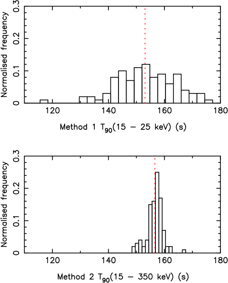
Figure 12: Histograms showing the scatter in $T_{90}$ estimates from repeated simulations at $z_{\rm sim}$ $=$ 6 for GRB 080319B, using both Method 1 (top panel) and Method 2 (bottom panel). Using both methods, all 100 repeats yielded detections using the BAT triggering algorithm. The red dotted line shows the average T₉₀ found in both cases.

The net result shown in Figures 8 and 10 is that the bulk of the simulations lie between $15\,{\rm s}<T_{90}<50\,{\rm s}$ at both $z=2$ and $z=6$, consistent with the mild evolution in $T_{90}$ seen in the observed Swift sample with redshifts (Figure 1). Note that at higher redshifts the reduced signal-to-noise ratio means that bursts may become undetected in some simulations. In the left panels of Figures 8 and 10 this is illustrated by the lines being plotted as solid while the burst remained detected in 90% of cases, and dotted for detection rates between 50% and 90%. Not surprisingly, this increased noise can lead to somewhat erratic evolution in the measured $T_{90}$ in some cases near the detection limit.

5.4 Evolution of $T_{c}$

The evolution of $T_{\rm c}$ with redshift is shown in the right-hand panels of Figures 8 and 10. As with $T_{90}$, the evolution can be tracked for a broader range in $z_{\rm sim}$ using Method 2, due to the improved signal to noise ratio of each light curve. In most instances $T_{\rm c}$ can be seen to increase even for bursts where $T_{90}$ reduces with increasing redshift. In some cases this rate of increase is significantly greater than would naively be expected due to time dilation: this can arise if the brightest peak happens to have a relatively soft spectrum, and hence declines more rapidly than the majority of the light curve due to band shifting as we simulate the burst at higher redshift.

Overall there are fewer instances of a decline in duration with redshift than was the case for $T_{90}$, supporting the proposition that $T_{\rm c}$ is less sensitive to the loss of pulses in the background noise.

Finally, the evolution with $z_{\rm sim}$ is smoother for Method 2 than Method 1. This is again largely due to the improved statistics of higher count rates.

6 Comparison with the known high-redshift population

Figure 13 shows the observed light curves of the known high-redshift population. Using the triggering algorithm described in §4.3 we verified that all six would have triggered BAT in both the 15–25 keV and 15–350 keV range. As our trigger algorithm only accounts for “rate triggers”, and does not implement an “image trigger” search, we are being conservative in comparison to BAT. It is likely that for a small range in simulated redshift shortly after a burst becomes too faint to cause a “rate trigger”, “image triggers” would be detected therefore recovering a higher fraction of the simulated burst population. The measured durations, $T_{90}$ and $T_{c}$, obtained for the high-redshift burst sample are included in Table 2. It is important to note at this point that we have not included GRB 050904, which was identified as an “image trigger” by BAT. We verified using our trigger algorithm that the BAT light curve could not have reached a “rate trigger” threshold using any combination of background and trigger durations.

Figure 13: 15–350 keV BAT light curves of the high-redshift subset. The light curves are binned at 1024 ms to allow clearer identification of structure within each. There is also a dashed line in each panel to show the zero count rate.

Table 2: The high-redshift GRB subset. Values of $T_{90}$ are those obtained from the standard BAT analysis in the energy ranges stated. $T_{c}$ was obtained using the algorithm described in §2.2. Missing entries in this Table are due to failure of the software to identify necessary bright structure in the light curves. (Redshifts from: 1. (Greiner et al., 2009), 2. (Tanvir et al., 2009), 3. (Cucchiara et al., 2011a), 4. (Tanvir et al., 2012), 5. (Levan et al., 2012))

GRB	Redshift	$T_{90}(15-25~{}{\rm keV})$	$T_{90}(15-350~{}{\rm keV})$	$T_{c}(15-25~{}{\rm keV})$	$T_{c}(15-25~{}{\rm keV})$
		(s)	(s)	(s)	(s)
GRB 080913	6.6951	8.26 $\pm$2.90	8.00 $\pm$0.95	…	4.10
GRB 090423	8.22	9.28 $\pm$2.29	10.62 $\pm$1.00	4.10	1.86
GRB 090429B	9.43	3.14 $\pm$2.29	5.57 $\pm$1.12	1.15	5.563
GRB 100905A	$\sim$7.25	…	3.39 $\pm$7.96	…	3.07
GRB 120521C	$\sim$64	24.64 $\pm$6.48	32.70 $\pm$7.96	4.42	2.88
GRB 120923A	$\sim$8.45	9.28 $\pm$3.24	27.46 $\pm$6.49	…	10.88

Should time dilation be considered to be the only mechanism affecting the observed high-redshift GRB sample, the durations of these bursts when moved to the local Universe would be considerably shorter. If a naïve factor of $1+z$ is applied, it can be shown that all six would have a rest frame duration of $T_{90}<5$ seconds.

We have already shown, however, that the evolution of duration is the result of several effects, not just time dilation. It is also important to note that one short GRB was included in the bright subset of bursts considered in detail. GRB 090510 may only be a single example, however it conforms with observational trends and the expectation that short bursts are not sufficiently bright to be detected at even moderate redshifts. This suggests that the high-redshift subset are unlikely to be short GRBs which have been misidentified due to time dilation of their prompt durations.

The prompt light curves of high-redshift GRBs are often considered to be the “tip of the iceberg” with weaker structure being undetectable. This makes it impossible to simulate high-redshift GRBs by blueshifting them into local Universe where this faint emission would become visible. To affect a successful comparison between GRBs at high- and low-redshifts, we therefore did the reverse: we simulated observed low-redshift GRBs at high-redshifts.

We took the average observed redshift of the high-redshift sample, $\bar{z}_{\rm high}=7.66$ (this excludes the image trigger GRB 050904, which would reduce the value to $\bar{z}_{\rm high}=7.46$). We then imposed an upper limit in redshift for those low-redshift bursts we would simulate at $\bar{z}_{\rm high}$. We included this upper limit ($z_{\rm orig}<4$) to mitigate the effects of any redshift dependent change in observed light curve morphology due to evolution in the progenitor population.

We then simulated all 114 bursts within the pulse-fitted sample meeting our redshift criterion ($z_{\rm orig}<4$) at $z_{\rm sim}=\bar{z}_{\rm high}$. Using the same process adopted for the bright subset, we repeated the simulation of each burst 100 times using Methods 1 and 2. We checked which of the simulated light curves for the 114 bursts would have caused a BAT trigger, using our triggering algorithm. Those light curves which were bright enough to trigger BAT at $z_{\rm sim}=\bar{z}_{\rm high}$ were then analysed to find both $T_{90}$ and $T_{c}$. For each simulated burst we averaged the values of $T_{90}$ and $T_{c}$ over the repeats which garnered a detection. These averages were then used in the statistical tests outlined below. It is important to note that only those bursts with detections in a minimum of 50% of their repeated simulations were retained.

To quantify whether the observed high-redshift population differs significantly from simulations of low-redshift bursts at comparable redshifts we performed K-S tests to compare the measured durations described in this work.

We were able to perform a K-S test on three of the four measures of duration. We were unable to compare the $T_{c}\left(15-25{\rm~{}keV}\right)$ values obtained via Method 1 as only three bursts in the high-redshift sample had sufficient signal to noise in the 15–25 keV band to yield a $T_{c}$ value. The results for these tests are reported as the top four lines of Table 3, whilst histograms corresponding to the three successfully tested durations are shown in Figure 14.

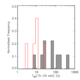
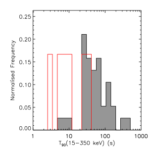
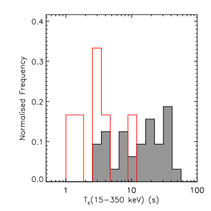
Figure 14: Histograms showing the normalised duration distributions of low-redshifts GRBs simulated at $\bar{z}_{\rm high}$ (filled grey) and the observed high-redshift (open red) samples for $T_{90}\left(15-25{\rm keV}\right)$ measured from Method 1 simulations (left), $T_{90}\left(15-350{\rm keV}\right)$ measured from Method 2 simulations (middle) and $T_{c}\left(15-350{\rm keV}\right)$ measured from Method 2 simulations (right) K-S tests.

Table 3: Results from K-S tests. The Method used (1 or 2) is shown in the first column. The second shows the duration being compared and the corresponding spectral range over which it was measured. $z_{\rm orig}$ describes the range of observed low-redshift GRBs that were simulated at $z_{\rm sim}$ for comparison with the high-redshift sample. For the last four tests, comparisons were being made to a moderate redshift sample, for which the $N_{2}$ population spanned $3<z_{\rm high}<4$. $N_{1}$ denotes the number of bursts in the simulated sample with a minimum of 50% detections at $\bar{z}_{\rm high}$ and successful output from the associated duration algorithm. $N_{2}$ corresponds to the number of observed high-redshift bursts with a measurable value of the relevant duration. $D$ is the K-S statistic, which measures the maximum distance between the cumulated distributions of the samples being compared, and $p$ is the resulting probability that the two samples arise from a common population. Rows in which the probability and maximum distance are missing are due to either $N_{1}$ or $N_{2}$ being too small to allow a K-S test.

Method	Duration	$z_{\rm orig}$	$z_{\rm sim}$	$N_{1}$	$N_{2}$	$D$	$p$
1	$T_{90}\left(15-25~{}{\rm keV}\right)$	$<4$	7.66	9	5	0.689	4.95 $\times$ $10^{-2}$
1	$T_{c}\left(15-25~{}{\rm keV}\right)$	$<4$	7.66	8	3	…	…
2	$T_{90}\left(15-350~{}{\rm keV}\right)$	$<4$	7.66	38	6	0.649	1.30 $\times$ $10^{-2}$
2	$T_{c}\left(15-350~{}{\rm keV}\right)$	$<4$	7.66	32	6	0.677	9.45 $\times$ $10^{-3}$
1	$T_{90}\left(15-25~{}{\rm keV}\right)$	$<2$	7.66	2	5	…	…
1	$T_{c}\left(15-25~{}{\rm keV}\right)$	$<2$	7.66	1	3	…	…
2	$T_{90}\left(15-350~{}{\rm keV}\right)$	$<2$	7.66	11	6	0.667	3.33 $\times$ $10^{-2}$
2	$T_{c}\left(15-350~{}{\rm keV}\right)$	$<2$	7.66	9	6	0.667	4.35 $\times$ $10^{-2}$
1	$T_{90}\left(15-25~{}{\rm keV}\right)$	$3<z_{\rm orig}<4$	7.66	2	5	…	…
1	$T_{c}\left(15-25~{}{\rm keV}\right)$	$3<z_{\rm orig}<4$	7.66	3	3	…	…
2	$T_{90}\left(15-350~{}{\rm keV}\right)$	$3<z_{\rm orig}<4$	7.66	12	6	0.667	2.98 $\times$ $10^{-2}$
2	$T_{c}\left(15-350~{}{\rm keV}\right)$	$3<z_{\rm orig}<4$	7.66	9	6	0.833	5.05 $\times$ $10^{-3}$
1	$T_{90}\left(15-25~{}{\rm keV}\right)$	$<2$	3.5	13	17	0.222	8.11 $\times$ $10^{-1}$
1	$T_{c}\left(15-25~{}{\rm keV}\right)$	$<2$	3.5	9	15	0.267	7.49 $\times$ $10^{-1}$
2	$T_{90}\left(15-350~{}{\rm keV}\right)$	$<2$	3.5	31	17	0.421	2.81 $\times$ $10^{-2}$
2	$T_{c}\left(15-350~{}{\rm keV}\right)$	$<2$	3.5	10	17	0.641	5.62 $\times$ $10^{-3}$

The results of the K-S tests in Table 3 show the statistics for comparison between the observed and simulated samples are better when using Method 2. This is simply due to the larger spectral range of BAT considered, as Method 2 allowed us to model all four of the standard BAT bands. Typically, the count rate for BAT GRBs peaks in channels 2 and 3, whilst Method 1 only simulates the softest channel. As a result the signal to noise ratios for Method 1 light curves were always poorer than their Method 2 counterparts.

Our null hypothesis, $H_{0}$, was that the measured durations of $T_{90}$ and $T_{c}$ for both the observed high-redshift GRB sample and simulations of all bursts with $z_{\rm orig}<4$ were drawn from the same parent population. Table 3 shows low values of $p$ for all performed K-S tests, indicating it unlikely that $H_{0}$ is true with significances between 2$\sigma$ and 3$\sigma$. Our most statistically significant result was for the Method 2 $T_{c}$ K-S test, where $p=9.45\times 10^{-3}$, indicating less than a 1% chance that the two samples are drawn from the same population. A 1% probability, for a high tail only test, corresponds to a 2.33$\sigma$ result. This is well below the standard 3$\sigma$ usually implemented, which corresponds to a probability of 0.13%.

Our initial K-S tests aimed to compare GRBs observed at $z\gtrsim 6$ to the largest possible sample of low-redshift events simulated at $z_{\rm sim}$. However, also displayed in Table 3 are further K-S tests where smaller subsets of the low-redshift sample are considered. Namely those where $z_{\rm orig}<2$ and $3<z_{\rm orig}<4$. In both cases the number of low-redshift GRBs that remained detectable when simulated at $\bar{z}_{\rm high}$ were too low to perform K-S tests on either the $T_{90}$ or $T_{c}$ durations as obtained via Method 1. For Method 2 simulated light curves, the additional K-S tests performed on measured $T_{90}$ have chance probabilities that are approximately a factor of two less significant than the original $z_{\rm orig}<4$ comparison. These increased probabilities are most likely due to the much decreased sample size, $N_{1}$, for both.

The light curves simulated via Method 2 have an increased chance probability when restricting the low-redshift sample to only $z_{\rm orig}<2$. Conversely, when only using busts for which $3<z_{\rm orig}<4$ the chance probability reduces by a factor of two, showing $p\sim 5\times 10^{-3}$. Both these and the $T_{90}$ K-S tests cast further doubt on any statistically significant difference between the low- and high-redshift samples, as none approach a 3$\sigma$ significance.

To further explore the evolution of measured durations as a function of redshift we also considered a more moderate change in redshift. We took all GRBs from our sample with $z_{\rm orig}<2$ and simulated them at $z_{\rm sim}=3.5$. These were then compared to the observed properties of all bursts in the redshift range $3<z<4$. The results of the statistical tests for both $T_{90}$ and $T_{c}$ measured from Method 1 and Method 2 light curves are shown in the bottom four lines of Table 3. As shown, the results from the Method 1 light curves have probabilities which firmly show we cannot reject $H_{0}$. The results from the Method 2 simulated light curves are similar to the previous K-S tests, chance probabilities $p\sim$2% and $p\sim$0.6% for $T_{90}$ and $T_{c}$, respectively.

While this draft was in an advanced state, GRB 130606A was discovered at $z=5.91$ (Chornock et al., 2013). The measured BAT $T_{90}\left(15-350~{}{\rm keV}\right)$ $\sim$280s with notable quiescent periods in the $\gamma$-ray light curve, which is much more in line with the expectations of what a time-dilated burst should be like (although we note this was intrinsically a particularly bright event). Were we to include GRB 130606A in our high-z sample the KS-test for $T_{90}$ from simulations produced using Method 2 would have produced a less significant probability of 3% that the observed and simulated high-z populations are from the same parent distribution. The corresponding K-S test for $T_{90}$ using Method 1 simulations result in a similarly increased probability of 8%.

Conversely, as the $T_{90}$ of GRB 130606A is largely comprised of quiescent times, $T_{c}$ remains short containing only fluence from the pulse complex at approximately 160 seconds after the initial trigger time. The K-S test using Method 2 simulations therefore has a reduced chance probability of 0.3%. This shows that while the traditional $T_{90}$ duration of GRB 130606A is longer, the bright core of emission denoting the time when the bursts is most active remains shorter and consistent with the other bursts in the high-redshift sample.

7 Discussion and conclusions

We first studied in detail the simulated evolution of a sample of 16 Swift GRBs at $z<2$ with high peak luminosities. By simulating their gamma-ray light curves as they would have been seen if the bursts had occurred at a range of redshifts ($z_{{\rm sim}}>2$), we have studied the primary mechanisms responsible in defining the measured prompt durations of GRBs.

We considered two methods of simulation, both of which are detailed in §4. Method 1 takes photons received by BAT, and considers those that would fall in the observed 15–25  keV band as the burst is moved to successively higher redshifts. This method has the advantage of being model independent, since it simply depends on the detected rate of hard photons. On the other hand, this reduced band-width is much less than the full energy range of BAT (15–350 keV) that is normally used to trigger and characterise GRB light curves, and the method is, of course, limited by the high-energy cut-off of BAT in the maximum redshift a given GRB can be re-simulated at.

Method 2 overcomes these deficiencies by modelling each light curve using the prompt pulse approach discussed in Willingale et al. (2010). From these models, high-energy BAT light curves can be simulated to arbitrarily high redshifts using the pulse temporal and spectral properties and typical background noise characteristics. This allows for more flexible and wider ranging comparisons, although is limited by the validity of the model.

With light curves in hand, we first determined whether the bursts would have triggered the BAT “rate-triggering” algorithm. Similarly, in comparing to the observed sample of high-redshift bursts we took care to ensure that they also exceeded one of the rate-trigger thresholds (in this work “image trigger” only bursts were discounted from consideration). If a burst satisfied the condition for triggering, we then determined its duration, using both the traditional $T_{90}$ and an alternative measure of the total duration of bright periods, so-called “core-time”, $T_{c}$.

Our implementation of the BAT trigger algorithm is not fully realistic, and in particular some bursts may be found using more elaborate BAT algorithms such as “image triggers”, which would be considered non-detections by us. However, because we apply our analysis consistently to all of the bursts (both known high-z, and bright bursts at low-z), rejecting any from either subset which fail our criteria, that should not introduce any major biases in our conclusions.

In general terms, we found that the measured durations of the simulated bursts varied with redshift in a way that depended on the initial structure of the light curve. While cosmological time-dilation always works to lengthen duration of the prompt emission, it is sometimes countered by the loss of some pulses as they drop below detectability, combined with the differing (and generally shorter) rest-frame duration measured in harder energy bands. Thus we might expect to find comparatively short durations for the simulated high-redshift bursts. This helps to explain the observed trend in the population average shown in Figure 1.

One concern in analyses of this sort is that Swift could be biased against finding highly redshifted bursts with time-dilated light curves due to the restricted periods (typically $<1000$ s) that the space-craft dwells in one location. This has been highlighted by the recent discoveries of a class of ultra-long GRBs at moderate redshifts (Gendre et al., 2013; Levan et al., 2013; Gruber et al., 2011). Those studies suggested that some ultra-long bursts ($T_{90}>$ 1500 s) could easily have be missed due to their emission being spread out in time. However, one important conclusion from our work is that the normal, bright LGRB population should not have observed durations of more than a few hundred seconds, even when time-dilated at high redshift, suggesting this potential bias is unlikely to be significant.

Both methods allowed us to make comparisons with the observed sample of very high-redshift Swift GRBs and bursts occurring in the more local Universe. By simulating all bursts for which the Willingale et al. (2010) pulse-fitting methodology had been applied, we considered a sample of 114 low-redshift ($z_{\rm orig}$) GRBs. These were simulated at $\bar{z}_{\rm high}$ to allow direct statistical comparison to the high-redshift subset. The results of the implemented K-S do suggest a marginally significant (99%) rejection of the hypothesis of no evolution of the GRB population duration distribution. Thus we have shown that the apparently short durations of high-z bursts to-date cannot simply be explained by band shifting and sensitivity considerations. On the other hand, the test we have performed is partially a posteriori in the sense that the short durations of the first few $z\gtrsim 6$ bursts was one of the motivating factors for conducting this study in the first place, and clearly it will require a larger sample in future to make completely robust statements.

We note that 31% (5/16) of bursts in our bright simulated sample were easily detectable at $z>10$. If such a population exists at high red shift instruments like the Swift/BAT can and may already have detected them although we were unable to follow-up the detection with a measurement of the redshift.

Appendix A Method 1 detailed description

To simulate BAT light curves, we obtained the event lists extracted for each burst using batgrbproduct. The additional required information included the BAT Ancillary Response File (ARF) and the actual observed redshift of the GRB in question, $z_{\rm orig}$.

As well as the number of source counts within each bin being reduced, the duration over which they are received is time dilated. Specifically, each simulated bin now has a duration of 64${F_{\rm z}}$ ms. As the arrival of each photon is a Poisson process we could not simply derive which fraction of the new bin size falls within a single 64 ms bin. Instead we took the extracted 15${F_{\rm z}}$–25${F_{\rm z}}$ light curve and calculated the total number of counts observed in each bin (by correcting for the bin size and the number of fully illuminated detectors). We also required a background. To find this we looked at the RMS scatter on the light curve, and added an offset equal to the square of this value, appropriate for Poisson noise.

Having the total number of counts, we then used $Q$ (where by definition, $Q\leqslant 1$) to consider whether each would remain in the light curve when the source was moved to $z_{\rm sim}$. To do so, we generated a random number $R_{1}$ from a uniform distribution ranging between 0 and 1. The value of $Q$ also took this range, with 1 corresponding to simulating the light curve at the redshift it was observed at. Any count for which $R_{1}$ $\leqslant$ $Q$ was retained in the light curve.

At this point we re–binned the light curve to the original 64 ms. To do so, we generated another random number, $R_{2}$. This was again drawn from a uniform distribution, ranging between 0 and 1. This number corresponded to the fraction of bin duration which had elapsed when the count arrived. The time of each event, $t_{\rm evt}$, is given as expressed in Equation 9, where $t_{\rm st}$ is the time at which the bin begins.

$$t_{\rm evt}={F_{\rm z}}\left(t_{\rm st}+0.064R_{2}\right).$$ (9)

Given a time for each count, they were re–sampled to 64 ms temporal binning, the background offset was removed, and the light curve was returned to the units of cts.s^-1.det^-1. This new light curve now contained the correct number of source counts. By scaling the total number of counts by a factor of $Q$, we also scaled the background was by the same quantity. This meant the total range in the fluctuations in the new background subtracted light curve was underestimated, and therefore an additional noise component was added. To correct the background, we calculated the variance on quiescent, non–slew times of both the transformed light curve and the original observed 15–25 keV light curve. The latter was also extracted from the available BAT data using the batbinevt routine. We compared these two variances, and found the difference, as shown in Equation 10.

$$\sigma_{\rm diff}^{2}=\sigma_{\rm orig}^{2}-\sigma_{\rm sim}^{2}.$$ (10)

A further series of random numbers was then generated. These were taken from a Gaussian distribution with mean of zero and standard deviation $\sigma_{\rm diff}$. We drew one random number per bin in the 64 ms simulated light curve. Each of these random numbers were added to their associated bin to increase the scatter on the simulated light curve to the level as seen in the observed 15–25  keV light curve. Having added this additional scatter, the resultant light curve contained the correct count rate and noise characteristics due to both the source and background.

Appendix B Simulating noise for Method 2

In this case the simulated light curves initially have no noise, so this must be added in a realistic way. To do so, the light curve was converted into a photon count rate per bin, then for each bin a Poisson distribution was randomly sampled, using the modelled number of counts as the expectation value of the distribution. This random number was then taken to be the simulated number of counts. This accounts for noise due to the source and to this we must add a background contribution. To achieve this we considered the observed light curve data from BAT in each of the four bands at the time during which the GRB was defined as active. We then considered the RMS value of errors on the light curve (excluding bright active regions) to find an average value of noise. This average noise was used as the standard deviation for a Gaussian distribution which had a mean of zero. Random numbers were drawn from this distribution and added to each bin of the four BAT channels. In principle the background variations could be both shot-noise and variations in, for example, astrophysical sources in the field. Our procedure accounts for any such variations that are reasonably fast, but not any slower variations (which would be correlated from bin to bin).

References

- Barthelmy et al. (2005) Barthelmy S. D., et al., 2005, Space Sci. Rev., 120, 143
- Belczynski et al. (2010) Belczynski K., Holz D. E., Fryer C. L., Berger E., Hartmann D. H., O’Shea B., 2010, ApJ, 708, 117
- Bromberg et al. (2013) Bromberg O., Nakar E., Piran T., Sari R., 2013, ApJ, 764, 179
- Burrows et al. (2005) Burrows D. N., et al., 2005, Space Sci. Rev., 120, 165
- Chornock et al. (2013) Chornock R., Berger E., Fox D. B., Lunnan R., Drout M. R., Fong W.-f., Laskar T., Roth K. C., 2013, ApJ, 774, 26
- Chornock et al. (2009) Chornock R., Perley D. A., Cenko S. B., Bloom J. S., 2009, GRB Coordinates Network, 9243, 1
- Cucchiara et al. (2011a) Cucchiara A., et al., 2011a, ApJ, 736, 7
- Cucchiara et al. (2011b) Cucchiara A., et al., 2011b, ApJ, 743, 154
- D’Avanzo et al. (2011) D’Avanzo P., D’Elia V., di Fabrizio L., Gurtu A., 2011, GRB Coordinates Network, 11997, 1
- de Ugarte Postigo et al. (2011) de Ugarte Postigo A., Castro-Tirado A. J., Gorosabel J., 2011, GRB Coordinates Network, 11978, 1
- Fenimore et al. (2003) Fenimore E. E., Palmer D., Galassi M., Tavenner T., Barthelmy S., Gehrels N., Parsons A., Tueller J., 2003, in Ricker G. R., Vanderspek R. K., eds, Gamma-Ray Burst and Afterglow Astronomy 2001: A Workshop Celebrating the First Year of the HETE Mission Vol. 662 of American Institute of Physics Conference Series, The Trigger Algorithm for the Burst Alert Telescope on Swift. pp 491–493
- Foley et al. (2005) Foley R. J., Chen H.-W., Bloom J., Prochaska J. X., 2005, GRB Coordinates Network, 3483, 1
- Fynbo et al. (2009) Fynbo J. P. U., et al., 2009, ApJS, 185, 526
- Gehrels et al. (2004) Gehrels N., et al., 2004, ApJ, 611, 1005
- Gehrels et al. (2006) Gehrels N., et al., 2006, Nature, 444, 1044
- Gendre et al. (2010) Gendre B., et al., 2010, MNRAS, 405, 2372
- Gendre et al. (2013) Gendre B., et al., 2013, ApJ, 766, 30
- Genet & Granot (2009) Genet F., Granot J., 2009, MNRAS, 399, 1328
- Gorbovskoy et al. (2012) Gorbovskoy E. S., et al., 2012, MNRAS, 421, 1874
- Greiner et al. (2009) Greiner J., et al., 2009, ApJ, 693, 1610
- Gruber et al. (2011) Gruber D., et al., 2011, A&A, 528, A15
- Kann et al. (2011) Kann D. A., et al., 2011, ApJ, 734, 96
- Klebesadel et al. (1973) Klebesadel R. W., Strong I. B., Olson R. A., 1973, ApJ, 182, L85
- Kocevski & Petrosian (2013) Kocevski D., Petrosian V., 2013, ApJ, 765, 116
- Kouveliotou et al. (1993) Kouveliotou C., Meegan C. A., Fishman G. J., Bhat N. P., Briggs M. S., Koshut T. M., Paciesas W. S., Pendleton G. N., 1993, ApJ, 413, L101
- Krühler et al. (2012) Krühler T., et al., 2012, A&A, 546, A8
- Levan et al. (2013) Levan A. J., et al., 2013, ArXiv e-prints
- Levan et al. (2012) Levan A. J., Perley D. A., Tanvir N. R., Cucchiara A., 2012, GRB Coordinates Network, 13802, 1
- Lü et al. (2012) Lü H.-J., Zhang B., Liang E.-W., Zhang B.-B., Sakamoto T., 2012, ArXiv e-prints
- McBreen et al. (2010) McBreen S., et al., 2010, A&A, 516, A71
- Meegan et al. (1992) Meegan C. A., Fishman G. J., Wilson R. B., Horack J. M., Brock M. N., Paciesas W. S., Pendleton G. N., Kouveliotou C., 1992, Nature, 355, 143
- Nakar (2007) Nakar E., 2007, Phys. Rep., 442, 166
- Norris & Bonnell (2006) Norris J. P., Bonnell J. T., 2006, ApJ, 643, 266
- Norris et al. (2000) Norris J. P., Marani G. F., Bonnell J. T., 2000, ApJ, 534, 248
- O’Meara et al. (2010) O’Meara J., Chen H. W., Prochaska J. X., 2010, GRB Coordinates Network, 11089, 1
- Paciesas et al. (1999) Paciesas W. S., et al., 1999, ApJS, 122, 465
- Paciesas et al. (2012) Paciesas W. S., et al., 2012, ApJS, 199, 18
- Page et al. (2007) Page K. L., et al., 2007, ApJ, 663, 1125
- Racusin et al. (2008) Racusin J. L., et al., 2008, Nature, 455, 183
- Reichart et al. (2001) Reichart D. E., Lamb D. Q., Fenimore E. E., Ramirez-Ruiz E., Cline T. L., Hurley K., 2001, ApJ, 552, 57
- Sakamoto et al. (2008) Sakamoto T., et al., 2008, ApJS, 175, 179
- Sakamoto et al. (2011) Sakamoto T., et al., 2011, ApJS, 195, 2
- Scargle (1998) Scargle J. D., 1998, ApJ, 504, 405
- Tanvir et al. (2009) Tanvir N. R., et al., 2009, Nature, 461, 1254
- Tanvir et al. (2012) Tanvir N. R., et al., 2012, GRB Coordinates Network, 13348, 1
- Vreeswijk et al. (2007) Vreeswijk P. M., et al., 2007, A&A, 468, 83
- Wiersema et al. (2008) Wiersema K., Tanvir N., Vreeswijk P., Fynbo J., Starling R., Rol E., Jakobsson P., 2008, GRB Coordinates Network, 7517, 1
- Willingale et al. (2007) Willingale R., et al., 2007, ApJ, 662, 1093
- Willingale et al. (2010) Willingale R., Genet F., Granot J., O’Brien P. T., 2010, MNRAS, 403, 1296
- Xu et al. (2009) Xu D., Fynbo J. P. U., Tanvir N. R., Hjorth J., Leloudas G., Malesani D., Jakobsson P., Wilson P. A., Andersen J., 2009, GRB Coordinates Network, 10053, 1
- Zhang et al. (2009) Zhang B., et al., 2009, ApJ, 703, 1696
- Zhang et al. (2007) Zhang B., Zhang B.-B., Liang E.-W., Gehrels N., Burrows D. N., Mészáros P., 2007, ApJ, 655, L25