Robust Quantification of Galaxy Cluster Morphology Using Asymmetry and Central Concentration

Abstract

We present a novel quantitative scheme of cluster classification based on the morphological properties that are manifested in X-ray images. We use a conventional radial surface brightness concentration parameter ($\rm{c_{SB}}$) as defined previously by others, and a new asymmetry parameter, which we define in this paper. Our asymmetry parameter, which we refer to as photon asymmetry ($\rm{A_{phot}}$), was developed as a robust substructure statistic for cluster observations with only a few thousand counts. To demonstrate that photon asymmetry exhibits better stability than currently popular power ratios and centroid shifts, we artificially degrade the X-ray image quality by: (a) adding extra background counts, (b) eliminating a fraction of the counts, (c) increasing the width of the smoothing kernel, and (d) simulating cluster observations at higher redshift. The asymmetry statistic presented here has a smaller statistical uncertainty than competing substructure parameters, allowing for low levels of substructure to be measured with confidence. $\rm{A_{phot}}$ is less sensitive to the total number of counts than competing substructure statistics, making it an ideal candidate for quantifying substructure in samples of distant clusters covering wide range of observational S/N. Additionally, we show that the asymmetry-concentration classification separates relaxed, cool core clusters from morphologically-disturbed mergers, in agreement with by-eye classifications. Our algorithms, freely available as Python scripts ({https://github.com/ndaniyar/aphot}) are completely automatic and can be used to rapidly classify galaxy cluster morphology for large numbers of clusters without human intervention.

1. Introduction

Clusters of galaxies are complex objects where many astrophysical processes are taking place. Cluster classification based on their X-ray morphology can help us understand the dominant physical processes in particular types of clusters, shed light on their formation histories, and give new insights into the evolution of both the large scale structure of the Universe (Allen et al., 2011) and the baryonic component of galaxy clusters (Böhringer & Werner, 2010).

Two distinctive features of galaxy clusters that are detectable in X-ray images are 1) cool cores and 2) departure from axial symmetry, presumed to arise from galaxy cluster mergers. Cool cores exhibit sharp central peaks in X-ray emission, while asymmetry manifests as secondary peaks, filaments, and clumps in X-ray surface brightness. It is believed that these features emerge at different stages of cluster evolution, and are outcomes of completely different physical processes that affect the entire intracluster medium (ICM). One important reason to classify cluster morphology is that we can explore any correlations between morphology and residuals in various cluster scaling relations, resulting in more robust estimates of, for example, galaxy cluster mass (M₅₀₀).

The substructure clumps in the X-ray emission are often associated with active processes of dynamical relaxation after mergers. For such clusters (with a high amount of substructure) the characteristic processes are turbulence (Vazza et al., 2011; Hallman & Jeltema, 2011), shocks, and cold fronts in the ICM (Markevitch & Vikhlinin, 2007; Hallman et al., 2010; Blanton et al., 2011), giant and mini radio halos (Cassano et al., 2010) and relics (Ferrari et al., 2008). After the process of relaxation is over, cool cores start to develop (Fabian et al., 1994; Peterson & Fabian, 2006; Hudson et al., 2010; McDonald et al., 2013), and the evolution of the ICM is governed by the processes of gas cooling and heating, AGN feedback (McNamara & Nulsen, 2007) and thermal conduction (Voit, 2011). We are still far from a detailed understanding of these processes, but their correlation with morphology is established both from observations and simulations. For example, observations suggest that more dynamically disturbed systems have weaker cool cores (Sanderson et al., 2009).

In this work, we propose a new classification scheme, based on the arrangement of galaxy clusters in the 2-dimensional plane of disturbance and cool core strength. As explained above, this choice of fundamental morphological parameters is observationally well-motivated. To choose the parameters that best quantify cool core strength and disturbance, we first formulate some requirements:

1. These parameters need to be objective, quantitative and reproducible.

2. The parameters should be model independent.

3. They should allow substructure analysis for low signal-to-noise (S/N) observations.

4. These parameters should be relatively insensitive to exposure time, the level of the X-ray background or a cluster’s angular size on the sky. A composite test that checks all these sensitivities together is simulating observations of a cluster at higher redshift.

5. The substructure parameters should agree with the human expert judgement.

The radial surface brightness profile of X-ray emission can be used to quantify the extent to which a cool core is present, although assigning clusters to categories (cool core vs. non cool core) is still a topic of discussion (Hudson et al., 2010; McDonald et al., 2013). We adopt here the concentration prescription of Santos et al. (2008), who showed that their implementation can discriminate between “strong”, “medium” and “no” cool cores. Importantly, in the context of the requirements listed earlier, the Santos et al. (2008) concentration parametrization is robust even for low S/N observations and is roughly model independent.

The quantification of “disturbance” is significantly harder. There is no simple physical (or mathematical) quantity that can measure “disturbance” or as it is usually called, the amount of substructure. Pinkney et al. (1996) list 30 different substructure tests and conclude that no single one is good in all cases. Two substructure statistics have, nevertheless, became popular recently: centroid shifts (Mohr et al., 1993) and power ratios (Buote & Tsai, 1995, 1996). Their popularity can be explained by their model-independence and ease of computation. They also satisfy, reasonably well, the requirements formulated above. For a more detailed review of various substructure statistics see Buote (2002); Böhringer et al. (2010); Rasia (2013); Weißmann et al. (2013). We present below a new substructure statistic that is superior based on the above requirements.

We stress that any substructure statistic should be suitable for high redshift clusters, with observations of poor quality. This is an area where the other substructure tests do not perform very well. Most morphological studies have been carried out for nearby clusters with high S/N X-ray images ($10^{5}$ counts per cluster being the typical value for these studies). However, large surveys or serendipitous discoveries of high-redshift clusters will yield images with, typically, only several hundred counts (e.g., McDonald et al., 2013). Thus, a reliable next-generation substructure statistic must perform equally well on low-S/N, high-redshift observations.

Here, we present a new substructure statistic, photon asymmetry ($\rm{A_{phot}}$), which quantifies how much the X-ray emission deviates from the idealized axisymmetric case. This statistic is somewhat similar to existing efforts to use the residuals after subtracting a beta-model fit (e.g. Neumann & Bohringer, 1997; Böhringer et al., 2000; Andrade-Santos et al., 2012) or double beta-model (Mohr et al., 1999). However, $\rm{A_{phot}}$ is model independent and specially designed to work well for observations with low photon counts.

In §2, we present the X-ray sample that has been used to develop our approach. §3 defines the various morphology measures that are compared in this work, while §4 explores performance using simulated data sets. Our results and conclusions are presented in §5 and §6, respectively. We defer an analysis of how these morphological parameters correlate with the scaling relations residuals to a future publication.

2. Sample and data reduction

2.1. Sample

To test our classification method and compare the properties of photon asymmetry to the properties of previously known substructure statistics, we used the high-z subsample of the 400 square degree galaxy cluster survey (abbreviated as 400d), which is a quasi mass-limited sample of galaxy clusters at $z>0.35$ serendipitously detected in ROSAT PSPC data (Burenin et al., 2007). The high-redshift subsample of 400d was published in Vikhlinin et al. (2009a) and consists of 36 clusters with $z>0.35$ which exceed a certain luminosity threshold which corresponds to $\approx 10^{14}M_{\sun}$ in mass (see Vikhlinin et al. (2009a) for details).

All clusters in the sample have been observed with the Chandra X-ray Observatory and used to constrain cosmological parameters in Vikhlinin et al. (2009a, b).

The reasons for choosing this cluster sample are:

1. A redshift range that covers $0.3\leq z\leq 0.9$, and is similar to the redshift range of both SZ surveys and next-generation X-ray surveys (e.g., eRosita), allowing extension to larger samples in the future.

2. High-resolution Chandra imaging which is very suitable for substructure detection. As we show in the paper, telescope resolution is very important to detect and quantify substructure.

3. A range of photon counts. Since our goal is to develop a substructure statistic that is maximally applicable to high-z clusters with low S/N observations, the high-z part of the 400d catalog is perfect for testing our substructure statistic.

4. The basic selection criterion is X-ray luminosity, which adequately samples the range of cluster morphologies and core properties. Thus the sample should be representative with respect to cluster morphological types.

2.2. Data reduction

We perform all industry-standard X-ray data reduction steps. We start with flare cleaned event2 files that are identical to those used by Vikhlinin et al. (2009a). Following many other cluster studies (e.g. Santos et al., 2008), we apply a 0.5 - 5.0 keV band filter which optimizes the ratio of the cluster to background flux. We chose to use a higher upper cut-off than what was used in many other studies (2 keV), because for massive clusters there is significant emission above 2 keV.

We detect point sources with an algorithm similar to wavdetect from the CIAO package (Fruscione et al., 2006) and replace the regions of point sources with a Poisson distribution with a mean value equal to the local background density of counts. In most cases this means that we add no counts in the region of the removed point source because the typical local background level is $\sim 10^{-2}$ counts per pixel.

We estimate the global background level from regions on the chip free of point sources, away from chip gaps, and sufficiently far away from cluster center (2-4 R₅₀₀ annulus)

We compute all morphological parameters directly from the raw event2 band-filtered files without additional binning or smoothing. All substructure statistics that we consider in this paper can be formulated in terms of sums over counts instead of integrals over surface brightness distributions as they are usually presented. We believe that this is the best way to perform statistical tests because any post-processing may distort and bias the statistic’s distributions.

We use exposure maps that include corrections for CCD gaps, spatial variations of the effective area, ACIS contamination, bad pixels and detector quantum efficiency.

We produce smoothed images of the clusters using an algorithm similar to asmooth (Ebeling et al., 2006), which chooses the appropriate smoothing scale adaptively for each count based on the local density of counts. These smoothed images are used for two (and only two) purposes:

1. Visualization for by-eye classification and by-eye comparison of the cluster’s relative ranking produced by various substructure statistics,

2. Generation of simulated cluster observations. See Section 5.2 for more details.

All the steps in the data reduction pipeline are automatic, but the results of each step were visually inspected. For the clusters that had several observations, we merged all observations that had the entire $R_{500}$ aperture on the CCD.

3. Classical morphological parameters/ substructure statistics

3.1. Power ratios

Power ratios were introduced in Buote & Tsai (1995, 1996) and have been widely used ever since (e.g. Jeltema et al., 2005; Ventimiglia et al., 2008; Cassano et al., 2010). They are able to distinguish a large range of morphologies, physically motivated and easy to compute (Jeltema et al., 2005). The method consists of a multipole expansion of the surface brightness and computes the powers in different orders of the expansion. The corresponding formulas are usually quoted as integrals over surface brightness, but since we prefer to work with individual counts and not smooth the surface brightness in any way, we replaced all the integrals with appropriately weighted sums over counts.

The powers are given by:

$$P_{0}=\left[a_{0}\ln(R_{ap})\right]^{2}$$ (1)

$$P_{m}=\frac{1}{2m^{2}R_{ap}^{2m}}\left(a_{m}^{2}+b_{m}^{2}\right),$$ (2)

where $R_{ap}$ is the aperture radius. The moments $a_{m}$ and $b_{m}$ are calculated using

$$a_{m}(R)=\sum_{r_{i}\leq R_{ap}}w_{i}r_{i}^{m}\cos(m\phi_{i})$$ (3)

and

$$b_{m}(R)=\sum_{r_{i}\leq R_{ap}}w_{i}r_{i}^{m}\sin(m\phi_{i}),$$ (4)

where $r_{i},\phi_{i}$ are the coordinates of the detected photon in polar coordinates and $w_{i}$ is its “weight” which is inversely proportional to the effective exposure at the given CCD location. The center of that polar coordinate system is chosen to set $P_{1}$ to zero.

In order to render the morphological information insensitive to overall X-ray flux, each of the angular moments $P_{m},m=1,2,3...$ is normalized by the value of $P_{0}$, forming the power ratios, $P_{m}/P_{0}$. The power ratios $P_{2}/P_{0}$, $P_{3}/P_{0}$, $P_{4}/P_{0}$ have been used to characterize cluster substructure (Jeltema et al., 2005). $P_{3}/P_{0}$ has been found to be the best characterization of “disturbance”.

Aperture choice is very important for power ratios as they are most sensitive to the substructure at the maximum radius. Values of 1 Mpc, 0.5 Mpc, $R_{500}$ have been used as aperture radii. We use $R_{500}$ as it allows more consistent comparison of clusters of different mass than a fixed physical scale as $R_{500}$ is a natural scale for clusters of all masses and redshifts. The other substructure statistics are also based on an $R_{500}$ aperture, therefore, our comparison of various substructure statistics is consistent.

As many authors have noted, the power ratios calculated by the formulas above give values for $P_{m}$ biased high due to photon noise. This can be easily seen in the case of a perfectly symmetrical cluster - the random distribution of the angles $\phi_{i}$, and nonnegativity of $P_{m}$, lead to a distribution of $P_{m}$ with nonzero mean. Different authors used different methods to account for these biases. We based our method of bias correction on the work of Böhringer et al. (2010), where the bias was computed by randomizing the polar angles for all collected photons, but keeping their radial distance fixed. The mean of the power $P_{m}$ of the mock observations obtained this way is interpreted as the typical photon noise contribution to the measurements of $P_{m}$ and subtracted from the $P_{m}$ of the real observation. We did not perform Monte-Carlo simulations for randomizing polar angles, because the mean of $P_{m}$ with randomized angles (uniformly distributed $\phi_{i}$) can be easily calculated analytically:

$$\begin{gathered}n_{m}=\langle a_{m}^{2}\rangle=\left\langle\left[\sum w_{i}r_{i}^{m}\cos(m\phi_{i})\right]^{2}\right\rangle\\ =\sum w_{i}^{2}r_{i}^{2m}\langle\cos^{2}(m\phi_{i})\rangle=\frac{1}{2}\sum w_{i}^{2}r_{i}^{2m}\\ \end{gathered}$$ (5)

We need to subtract this value from both $a_{m}^{2}$ and $b_{m}^{2}$ which results in the following formula for $P_{m}$.

$$P_{m}=\frac{1}{2m^{2}R_{ap}^{2m}}\left(a_{m}^{2}+b_{m}^{2}-2n_{m}\right),$$ (6)

After bias correction the background counts do not contribute to the powers $m\neq 0$, but still contribute to $a_{0}=\sum w_{i}$. To make $P_{0}$ and, consequently the ratios background independent, we need to also subtract the background contribution from $a_{0}$:

$$a_{0}=\sum w_{i}-w_{\mathrm{bkgr}}(R_{ap}),$$ (7)

where $w_{bkgr}(R_{ap})$ is the expected total weight of all background photons within the aperture $R_{ap}$.

3.2. Centroid shifts

Centroid shift is another popular measure of “disturbance” of clusters. It is defined by the variance of “centroids” obtained by minimization of $P_{1}$ within 10 apertures($r\leq n\times 0.1\,R_{500}$, with n = 1,2..10). The value of centroid shifts is expressed in units of $R_{500}$ which makes it a dimensionless quantity. Centroid shifts are defined slightly differently by different authors (See Mohr et al., 1995; Poole et al., 2006; O’Hara et al., 2006; Böhringer et al., 2010). Here we used

$$w=\left[{1\over N-1}\sum_{i}\left(x_{i}-\langle x\rangle\right)^{2}\right]^{1/2}\times{1\over R_{500}},$$ (8)

where $x_{i}$ is the position of the centroid of a given aperture.

3.3. Concentration

Concentration parameter is defined as the ratio of the peak over the ambient surface brightness. Concentration has been widely applied to X-ray images (Kay et al., 2008; Santos et al., 2008, 2010; Cassano et al., 2010; Hallman & Jeltema, 2011; Semler et al., 2012) and proved useful in distinguishing cool-core (CC) from non-cool-core (NCC) clusters.

We adopted the definition of concentration provided by Santos et al. (2008):

$$c_{SB}=\frac{\mathrm{Flux}(r<40\mathrm{kpc},\;0.5\mathrm{keV}<E<5\mathrm{keV})}{\mathrm{Flux}(r<400\mathrm{kpc},\;0.5\mathrm{keV}<E<5\mathrm{keV})}$$ (9)

The radii 40 and 400 kpc were chosen to maximize the separation between CC and NCC clusters. We computed concentration around the brightness peak as defined in Section 4.4, the same center that we used for photon asymmetry. Complete details on the stability of the concentration parameter can be found in Santos et al. (2008).

4. Photon asymmetry

In this section we will describe our proposed morphological classifier, namely photon asymmetry.

4.1. Optical asymmetry and the motivation for photon asymmetry

In optical astronomy the asymmetry parameter is a part of the “CAS” galaxy classification scheme which stands for concentration (C), asymmetry (A) and clumpiness (S) (Conselice, 2003). Asymmetry quantifies the degree to which the light of an object (galaxy) is rotationally symmetric. It is measured by subtracting the galaxy image $I_{180}$ rotated by $180^{\circ}$ from the original image $I_{0}$ (Conselice, 2003):

$$A=\frac{|I_{0}-I_{180}|}{I_{0}}$$ (10)

This definition tests central (or mirror) asymmetry, i.e. whether the image is invariant under a “point reflection” transformation (which is equivalent to rotation by $180^{\circ}$ around the central point). Although this definition of asymmetry has been applied to X-ray images of clusters before (e.g. Rasia, 2013), it is only reliable for observations where the number of counts in each (binned) pixel is $\gg 1$. This condition is not satisfied for most cluster observations.

One can come up with a similar definition of circular or axial asymmetry which would test whether the image is invariant under rotation by arbitrary angle around the central point. That would involve finding the average intensity of the image in concentric annuli, and comparing local intensity with the average intensity in the annulus.

$$A=\int_{0}^{R}rdr\int d\phi\left(I(r,\phi)-\overline{I(r)}\right)^{2}$$ (11)

This could also be a good measure of substructure and indeed people have tried to apply similar ideas for substructure statistics (e.g. Andrade-Santos et al., 2012).

The above definitions of asymmetry, both (10) and (11), are hard to implement for distant clusters whose observations have fewer counts. We could generate smoothed images of clusters and apply the above definitions to these images, but that can generate biases. The large radial variations in surface brightness and the presence of substructure deny the ability to choose a single, global optimal smoothing scale. We cannot use an adaptive scale either, because asymmetry is then strongly dependent on the details of the adaptive smoothing algorithm. Also, by producing smoothed images (with either a fixed or adaptive scale), we effectively introduce some model-dependent prior on cluster structure. We would prefer, however, to only use objective information: the positions (and possibly energies) of the detected photons.

Fortunately, there is a way to adapt the definition of asymmetry so that it can be computed efficiently in the limit of low photon counts, which we present in this paper. This adaptation is possible for both central and axial asymmetry. Central asymmetry might seem preferable, because it would have a zero value for a relaxed, but elliptical cluster. However, in our sample with few counts and ill-defined ellipticities, the values of axial and central asymmetries correlate strongly. Additionally, axial asymmetry is conceptually simpler for our statistical framework, so we concentrate on it for this paper.

Our strategy for adapting Eq. (11) to the case of few counts with known coordinates is the following. We split the image into a few annuli, and check whether the surface brightness is uniform in each of these annuli. In the limit of few counts, this is the same as checking whether these counts are uniformly distributed in the annulus. This amounts to checking that their polar angles are uniformly distributed in the $0\leq\phi<2\pi$ range.

4.2. Photon asymmetry within an annulus

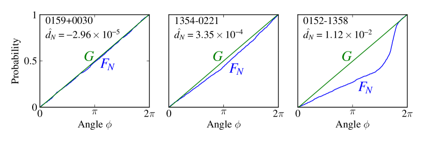
Figure 1.— The method described in this paper compares the observed cumulative probability distributions of the angular positions of photons (F_N), to that of a uniform distribution (G). This Figure shows empirical $F_{N}$ and uniform $G$ distribution functions in the outermost annulus for 3 progressively more disturbed clusters (0159+0030, 1354-0221, and 0152-1358). The more disturbed clusters manifest greater differences between $F_{N}$ and $G$ and correspondingly higher values of distance metric $d_{N}$.

To assess the degree of nonuniformity of the angular distribution of the counts, we use Watson’s test (Watson, 1961). Watson’s test compares 2 cumulative distribution functions. Other members of this family of non-parametric tests for the equality of distribution functions include the well-known Kolmogorov-Smirnov test as well as less well-known Cramer-von Mises and Kuiper’s tests. For the reasons explained in the Appendix, Watson’s test is the only one that works in our specific situation. Unfortunately, Watson’s test is only able to test the null hypothesis, i.e. compute the probability that the given sample is drawn from the assumed distribution. Our case is slightly different - we know that our sample (of counts as function of polar angles) is not drawn from the uniform distribution, so, in principle, goodness of fit tests are not applicable to our case. However, as we show in the Appendix, we can interpret the value of Watson’s test as the estimate of the distance between the true underlying distribution function and the assumed distribution function.

Let us consider the photons that arrive in an annulus $R_{in}<r<R_{out}$ relative to the cluster center. The specific definition of these annuli will be discussed in Section 4.3. Let $\Phi$ be a polar angle (random variable) of a cluster photon in the chosen coordinate system, centered on the cluster, and $\phi_{1},\phi_{2},\cdots,\phi_{N}$ are the polar angles of the observed photons in the annulus ($N$ = total number of observed photons in the annulus). Then we will define:

$$F(\phi)=\mathrm{Prob}(\Phi\leq\phi)$$ (12)

as the true angular (cumulative) distribution function and

$$\begin{gathered}F_{N}(\phi)=\frac{1}{N}\sum\left\{\begin{array}[]{ll}1,&\textrm{ if }\phi_{i}\leq\phi\\ 0,&\textrm{ otherwise}\end{array}\right.\end{gathered}$$ (13)

as the measured (empirical) distribution function. Being distribution functions on a circle, $F$ and $F_{N}$ also depend on the arbitrary starting point $\phi_{0}$ which we write as

$$\begin{gathered}F=F(\phi;\phi_{0})\\ F_{N}=F_{N}(\phi;\phi_{0}).\end{gathered}$$ (14)

We can now introduce Watson’s statistic $U_{N}^{2}[F_{N},F]$ as

$$\begin{gathered}U_{N}^{2}[F_{N},F;\phi_{0}]=N\int\Big{(}F_{N}(\phi;\phi_{0})-F(\phi;\phi_{0})\Big{)}^{2}dF\\ U_{N}^{2}[F_{N},F]=\min_{\phi_{0}}U_{N}^{2}[F_{N},F;\phi_{0}],\end{gathered}$$ (15)

i.e. $U_{N}$ is the minimum value of integrated squared difference between $F_{N}$ and $F$ over possible starting points $\phi_{0}$.

The greater the value of $U_{N}^{2}$ the less likely that $F_{N}$ is produced by drawing from $F$. In our case $F$ is unknown, but we can test how likely it is that $F_{N}$ is drawn from another distribution $G$ which represents an idealized axisymmetric source. ($G$ would be uniform in the absence of instrumental imperfections)

$$U_{N}^{2}[F_{N},G]=N\min_{\textrm{origin on the circle}}\int(F_{N}-G)^{2}dG.$$ (16)

Interestingly, it is possible to interpret $U_{N}^{2}[F_{N},G]/N$ as the distance between $F$ and $G$:

$$U_{N}^{2}[F_{N},G]/N=\textrm{distance}(F,G)+\frac{1}{12N}+\textrm{Noise},$$ (17)

where the bizarre term $1/12N$ comes from the properties of the statistic distribution under the null hypothesis. The detailed derivation of (17) is presented in the Appendix. Here we would like to note that the mean value of Noise is smaller than $1/12N$ for the relevant values of $N$, therefore

$$\hat{d}_{N}=U_{N}^{2}/N-1/12N$$ (18)

is an estimator of $\textrm{distance}(F,G)$, the distance between the observed and uniform distributions of photons in the annulus. The variance of this estimator scales as $1/N$, so that we can get better estimate of the distance as N increases.

The method is illustrated in Fig. 1 where we show $F_{N}$, $G$, and the value of $\hat{d}_{N}$ in the outermost annulus for 3 progressively more disturbed clusters. The more disturbed clusters manifest greater differences between $F_{N}$ and $G$ and, consequently, higher values of $\hat{d}_{N}$.

As we are interested in the distance between the observed and a uniform distribution of cluster-only photons (as opposed to cluster and background photons), we additionally need to multiply that distance by the squared ratio of total counts $N$ to cluster counts $C$ in that annulus. As the number of cluster counts $C$ is not directly observable, we estimate it by subtracting the expected number of background counts in the annulus from the total counts $N$. The resulting background-corrected expression

$$\hat{d}_{N,C}=\frac{N}{C^{2}}\bigg{(}U_{N}^{2}-\frac{1}{12}\bigg{)},$$ (19)

is an estimate of the distance between the true photon distribution and the uniform distribution. (see Appendix for details)

4.3. How to choose the optimal annuli

The first step in choosing optimal annuli is to select the maximum aperture radius. $R_{500}$ is a good choice, because cluster X-ray emission is typically indistinguishable from the background beyond this radius. Also, we exclude the region $r<0.05R_{500}$ from the analysis because pixelation artefacts at small radii distort Watson’s statistic.

Second, we need to choose the number of annuli inside this $0.05R_{500}<r<R_{500}$ region. One can use any number of annuli for the computation of asymmetry. The tradeoff is between the asymmetry S/N in each individual annulus and radial resolution. We found that it is desirable to have at least a few hundred counts in each annulus, so we used 4 annuli for our sample of clusters. This optimization may be different for a cluster sample with different number of counts.

Finally, we need to choose the radii of these annuli. The relative uncertainty of asymmetry is estimated to be $\sqrt{N}/C$, where $N$ is the total number of counts, and $C$ is the number of cluster counts. The radial binning should be chosen carefully, because low numbers of $N$ or $C$ in any bin inflate the uncertainty. This is a nontrivial task as the radial brightness profile is very different between clusters. We choose the radial binning to achieve a uniform relative uncertainty in asymmetry, for each annulus, across the clusters in our training set. The following choice of boundaries in units of $R_{500}$: 0.05, 0.12, 0.2, 0.30, 1, leads to the most uniform uncertainty across bins. We caution that applying this technique to X-ray survey instruments or data sets that exhibit a broader PSF than Chandra’s 0.5 arcsec FWHM will require a careful reevaluation of radial binning, sence we desire annuli widths $dr\gg\rm{FWHM}$.

The last step in the computation of photon asymmetry is to combine the values of asymmetry from the 4 annuli. We use a weighted sum of distances from each annulus $\hat{d}_{N_{k},C_{k}}$ (see Eq. (19), $k$ numbers the annuli, $N_{k}$ and $C_{k}$ are the total and cluster counts in $k$-th annulus) with a weight equal to the estimated number of cluster counts $C_{k}$ in that annulus.

$$A_{phot}=100\sum_{k=1}^{4}C_{k}\hat{d}_{N_{k},C_{k}}/\sum_{k=1}^{4}C_{k}$$ (20)

We introduced a multiple of 100 into the definition of $\rm{A_{phot}}$ to bring all the asymmetries to a convenient range $0<\rm{A_{phot}}\lesssim 3$. The resulting quantity is independent of exposure and background level.

4.4. Cluster centroid determination

The standard prescription for optical asymmetry is to choose the center that minimizes asymmetry. However this method is prone to producing values of asymmetry that are biased low. This effect is especially noticeable in our resamplings with very low number of counts.

We based our choice of centroiding on three considerations: 1) we favor a centroid choice that is independent of the asymmetry computation, 2) if the cluster possesses a strong core, we use that feature to define the cluster center, and 3) by assigning the cluster center to a high S/N region of the image, we can compute asymmetry in annuli at high S/N.

Based on these requirements, we chose the center to be the brightest pixel after convolution with a Gaussian kernel with $\sigma=40$ kpc. At $z=1$, a single Chandra pixel corresponds to about 4 kpc, and the Chandra PSF FWHM is of order 2 pixels, so the smoothing scale is much coarser than Chandra angular resolution.

The centroid defined as a convolution with a Gaussian kernel is not very sensitive to the size of this Gaussian kernel. We chose the kernel size to be 40kpc to be consistent with our definition of concentration. We use this centroid for both asymmetry and concentration. We stress that the Gaussian-convolved image is used only for centroiding, not for computation of any substructure statistics.

4.5. Additional remarks

The $A_{phot}$ parameter can be applied beyond X-ray observations. In fact, a quantity defined exactly the same way can be used for optical observations of clusters if we replace the coordinates of each photon with the coordinates of a member galaxy. Additionally, each galaxy can be given a weight that depends on its optical luminosity (e.g. w $\sim\log$ luminosity). These weights can replace the ones in eq.(13), so that F remains a proper distribution function. In this case the equations (13)-(20) remain valid yielding a parameter that describes the asymmetry of the galaxy distribution within a cluster derived from optical observations.

5. Simulated observations and determination of uncertainties

5.1. Simulated observations

We now address the questions of 1) sensitivities of substructure statistics to observation parameters, and 2) uncertainties of these substructure statistics, by calculating them for simulated observations with the desired parameters (such as exposure or background level). The idea of using simulated observations in similar ways goes back to the works of Buote & Tsai (1996); Jeltema et al. (2005); Hart (2008); Böhringer et al. (2010). Generating these simulated observations is straightforward if we have the map of the true cluster surface brightness (or, more precise, cluster brightness multiplied by CCD exposure map) - we would draw each pixel value from the Poisson distribution with the mean equal to that brightness. As we don’t know that true underlying brightness distribution, we use instead our best approximation to it, which is the result of an adaptive smoothing algorithm.

To simulate changing the exposure, before drawing from Poisson distribution, we need to multiply the surface brightness map by a constant; to change the level of background, we need to add a constant to the surface brightness map; to change the telescope PSF, we need to convolve the existing brightness map with the new PSF (the real Chandra PSF is negligibly small).

To simulate how the clusters would look if they were moved to a greater redshift, we need to calculate the expected X-ray flux from that cluster, rescale the number of observed counts accordingly, change the image spatial scale (which is a small correction as angular diameter distance doesn’t change much from z = 0.3 to 1), and then increase the amount of the background to its old value. The only tricky part in this process is the calculation of the new cluster flux which should include the change in the luminosity distance, and the K-correction (Hogg et al., 2002) that compensates for the shift in the cluster emission in the observed frame.

$$\frac{\mathrm{Flux}_{\mathrm{new}}}{\mathrm{Flux}_{\mathrm{old}}}=\frac{D_{L,\mathrm{old}}^{2}}{D_{L,\mathrm{new}}^{2}}\frac{K(z_{\mathrm{new}})}{K(z_{\mathrm{old}})}$$ (21)

Since we don’t need to simulate this very precisely – we only want to get an idea of how it affects the substructure measures – we use a simple approximation to Santos et al. (2008) results for 0.5-5 keV energy band:

$$K(z)=\frac{1}{1+2z}$$ (22)

5.2. Uncertainties

To estimate the uncertainties of the various substructure statistics, we used the above-described algorithm to generate 100 mock observations with exactly the same exposure and background level as in the original observations, but varied noise realization. Then we computed the substructure statistics for these samples, and found the median, the 16th lowest and the 16th highest observed value in the sample. We treat the median as the characteristic central value of statistic for this set of mock observations, and the interval between 16th lowest and the 16th highest observed value as the 1$\sigma$, or 68% confidence interval. Using order statistics for the central value and the confidence interval is the most sensible choice for us, because the distributions for any substructure statistic values are asymmetric and extremely heavy tailed. The statistic value obtained from the real observation didn’t always fall within this confidence interval for two reasons. First, as this is only a 68% confidence interval, we expect approximately $1/3$ of all points to be outside of the $1\sigma$ range. Second, the resampling process tends to overestimate the cluster substructure. This arises because our smoothed surface brightness maps do contain some residual noise due to Poisson statistics from the cluster and the background, and we then inject an additional component of shot noise when computing a fake cluster observations. Thus, the value of the statistic for mock observations may be biased, and the confidence intervals for the mock observations and the real ones are not expected to coincide. However, we expect that the true surface brightness and the inferred one would produce the samples of statistic values with similar variances. Therefore, we can use the variability of the simulated sample to determine the size of the error bars, but should center the error bars on the statistic value obtained for the real observation instead of the mean of the sample. A similar method of calculating uncertainties from simulated observations was used by Böhringer et al. (2010).

The method described above provides robust uncertainty estimates, but requires complicated machinery that generates adaptively smoothed maps and mock observations. We have used this machinery to perform substructure sensitivity tests, but one may want to use simpler uncertainty estimation methods when only interested in the uncertainty of asymmetry for a given observation. Therefore, we developed a simplified uncertainty estimation method which does not use the adaptive smoothing algorithm. We used subsampling method to determine the scatter in the measured asymmetry values. We generated mock observations that take a random half of the counts from the original observation and computed substructure statistics from them. The scatter in the resulting asymmetry values is expected to $\sqrt{2}$ larger than what we would obtained for the full sample, so we need to reduce these error bars by $\sqrt{2}$. This method avoids additional assumptions about clusters introduced by the adaptive smoothing algorithm, and is significantly simpler in implementation. We compared the error bars produced with both methods (Fig. 2), and found them to be similar.

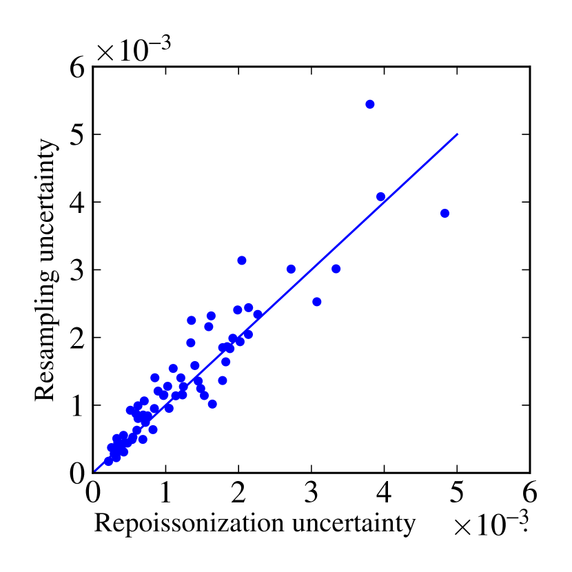
Figure 2.— Comparison of A_phot uncertainties computed by two different methods. The horizontal axis represents uncertainties estimated by “repoissonization” (Weißmann et al., 2013). The vertical axis represents uncertainties estimated by resampling half of the observation photons with replacement. The two methods agree well, suggesting that the simpler of the two (resampling) is a sufficient representation of the “true” uncertainty.

We also produced samples of 100 mock observations each where we changed one parameter of observation (such as exposure) for our sensitivity tests. In these tests, we viewed the adaptively smoothed images of clusters as the true surface brightness distributions in the sky. Unlike the previous group of simulations, here the true value of the statistic is not relevant. The median and the 68% confidence interval for each such sample represent how the statistic reacts to the corresponding change in the parameter of observation (such as exposure).

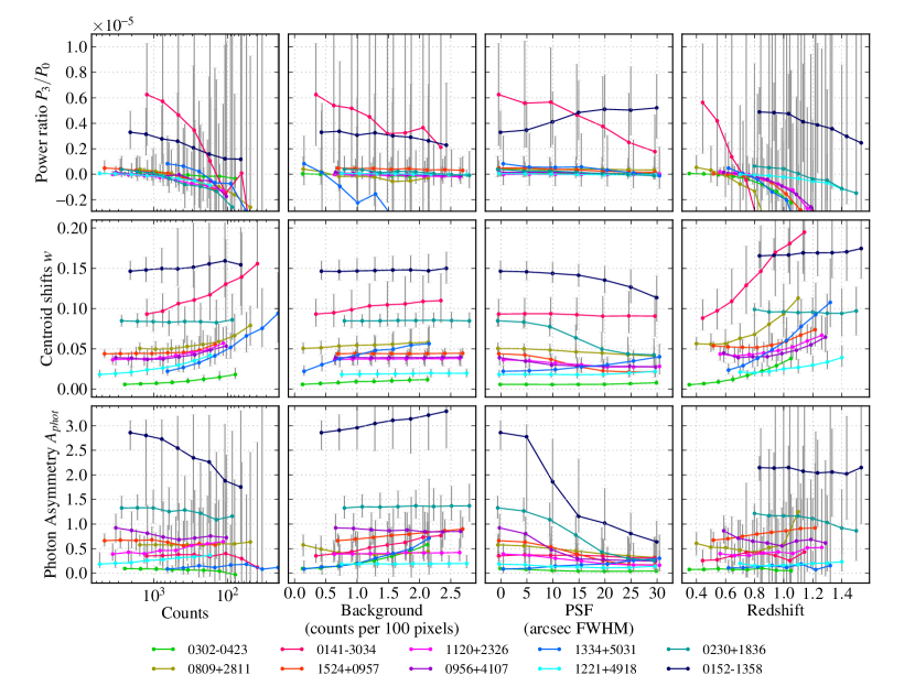
Figure 3.— Sensitivity of 3 substructure statistics: power ratios, $P_{3}/P_{0}$ (1st row), centroid shifts, $w$ (2nd row), and photon asymmetry, $\rm{A_{phot}}$ (3rd row) to the quality of observations: number of counts within $R_{500}$ (1st column), background level (2nd column), telescope PSF (3rd column), and cluster redshift at fixed exposure (4th column). Only a representative subset of the clusters is shown in this Figure - the complete sample is shown in Fig. 4. An idealized morphological statistic would be insensitive to the quality of observations, i.e. all the lines should be parallel to x-axis. The photon asymmetry parameter presented in this paper shows better stability and better resolving power for observations of poor quality than commonly-used power ratios and centroid shifts. The names of the clusters are identical to those used in Vikhlinin et al. (2009a).

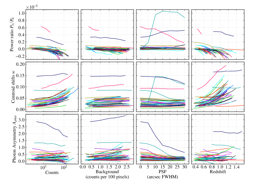
Figure 4.— Similar to Fig. 3, but now showing the full sample of 36 clusters from Vikhlinin et al. (2009a). Uncertainties are excluded in this plot in order to reduce clutter – see Fig. 3 for a subset of these clusters with uncertainties. The points where uncertainties exceed the entire dynamic range for the corresponding substructure statistic are excluded from the plots.

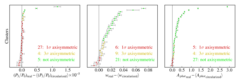
Figure 5.— This figure demonstrates how well each of the three substructure statistics examined in this paper is able to discriminate between the true photon distribution and the idealized case of axisymmetry for each of the 36 clusters in Vikhlinin et al. (2009a). For each cluster, we compare the measured substructure statistic to the expectation for a perfectly smooth, axisymmetric source. Horizontal bars represent 1$\sigma$ confidence intervals. The red points indicate clusters that are within $1\sigma$ of axisymmetry and, thus, are indistinguishable from the unrealistic case of perfect axisymmetry. The yellow and green points indicate clusters that are within $3\sigma$ and $>$3$\sigma$ of axisymmetry, respectively. Since no cluster should be perfectly symmetric, this plot demonstrates the sensitivity of each statistic to low levels of substructure, with A_phot performing the best overall.

6. Results and Discussion

6.1. Sensitivity of morphological parameters to data quality

An important test for any substructure statistic is its insensitivity to the observational S/N. Here we present sensitivity tests of two currently-popular substructure parameters (centroid shifts and power ratios $P_{3}/P_{0}$) and the new one introduced in this paper (photon asymmetry, $\rm{A_{phot}}$). We conducted 4 tests that degraded the observations in different ways, namely 1) reduced the number of photons (exposure), 2) increased the level of background, 3) “blurred” the observation with larger PSF (or, alternatively, decreased the cluster’s angular size), and 4) altered the observations in all mentioned ways, simulating an observation of the same cluster with the same exposure as if it was at higher redshift.

The plots of all sensitivities are presented in Figures 3 and 4, with different statistics in rows and sensitivity tests in columns. Fig. 3 shows both median values of statistics and $1\sigma$ confidence intervals, but only for a subset of representative clusters, while Fig. 4 shows only median values of statistics that we obtained in our Monte-Carlo simulations (see Sec. 5.2). We chose to present plots of only $P_{3}/P_{0}$ for power ratios, because $P_{3}/P_{0}$ is believed to be the best indicator of substructure. The plots of $P_{2}/P_{0}$ and $P_{4}/P_{0}$ look qualitatively very similar.

All statistics show relative insensitivity to the number of cluster counts, at levels above $\sim$ 2000 counts. However, in the low counts regime, both power ratios and centroid shifts show strong biases. The power ratio tends to be biased low for all clusters. Centroid shifts tend to be biased high, more so for clusters that do not show significant substructure. Each cluster seems to have its own threshold value in number of counts, so that centroid shifts are stable when there are sufficient cluster counts, but start to increase as the simulated number of counts falls below this threshold value. This behavior of centroid shifts is not surprising, because the statistical error of finding a centroid of a few photons should scale as one over the square root of the number of photons, unless there are significant secondary emission peaks that “pin” centroids of certain radii. In other words, although this bias has a similar behavior for many clusters, it cannot be corrected simply as a function of number of counts – it also depends on the morphology (Weißmann et al., 2013).

Centroid shifts, perhaps unsurprisingly, are the most stable statistic with respect to background levels. The determination of centroid is simply insensitive to a uniform background (unless there are so few counts that the $1/\sqrt{N}$ effect described in the previous paragraph starts playing a role). Power ratios are relatively stable with respect to background levels. (Although they become consistent with zero for every cluster in the sample after even a moderate background increment due to increased uncertainty.) Asymmetry is insensitive to background levels as long as a reliable estimate of cluster counts is possible in each annulus. However, when the square root of the total counts becomes comparable to the cluster counts, the estimate of cluster counts may become close to zero (or even negative). This unphysical estimate of cluster counts, being in the denominator in Eq. (19), drives the statistic to high absolute values. This is a drawback of $\rm{A_{phot}}$, which could be fixed by a more careful separation of background and cluster counts.

None of the statistics are stable against PSF increase because at $30^{\prime\prime}$ PSF the substructure is completely washed out and undetectable by any method. Asymmetry has a stronger sensitivity to PSF, because it probes the non-uniformity of the photon distribution on all angular scales, starting from the lowest Fourier harmonics to the highest. Power ratio $P_{3}/P_{0}$, on the other hand, is only sensitive to the third Fourier harmonic. It is interesting that the PSF has a much stronger influence on any substructure statistic than does the number of counts. This observation suggests that for substructure studies a telescope’s angular resolution is more important than its effective area.

The redshift test is the most challenging: the luminosity distance increases very fast, and the K correction adds to the flux dimming, effectively making the high-z simulated observations dominated by the background. Fluctuations in background increase variability of centroid estimation, driving centroid shifts to higher values. (A similar effect is demonstrated by sensitivity to cluster counts.) The power ratio median “dives” down to negative values (again, similar to counts test). Additionally, power ratio uncertainties increase very quickly, which is the result of background correction (subtraction of two nearly equal terms in Eq. (6)). Photon asymmetry also suffers from background correction, but overall shows less sensitivity to simulated redshift than either power ratio or centroid shifts.

What sets photon asymmetry apart from power ratios and centroid shifts is much smaller relative uncertainties. Unlike power ratios and centroid shifts, photon asymmetry is typically further than one standard deviation away from zero. So, photon asymmetry is capable of separating relaxed and slightly unrelaxed cluster populations in the case of observations with even a few hundred X-ray counts. To demonstrate that photon asymmetry is better than its competitors at distinguishing the clusters that are inconsistent with axisymmetric sources in the low S/N regime, we calculated the number of clusters in our sample that are 1$\sigma$ consistent with circularly symmetric sources.

In order to compare the statistical significance of three different substructure parameters (photon asymmetry, centroid shifts and power ratios), for each cluster we generated a set of idealized, axisymmetric clusters. This was done by retaining the exact radial location for each of the N detected photons for each cluster, but with a random realization of polar angles for each photon’s position. We then computed the relevant substructure metric. For each cluster we subtracted the mean of the parameter values computed from the fake circular clusters from that obtained from the actual cluster. We also assigned the scatter in the fake measurements as the uncertainty, for each cluster. Figure 5 shows departure from the circular case, with photon asymmetry clearly achieving a more significant determination of cluster substructure. Confidence intervals overlapping with 0 (red points) mean that the cluster indistinguishable from the axisymmetric case. The yellow points indicate clusters that are within $3\sigma$ of axisymmetry.

The number of clusters that are statistically inconsistent (at $3\sigma$) with the idealized, axisymmetric case, as determined by different substructure statistics, are as follows:

• Power ratio $P_{3}/P_{0}$: 5 (out of 36)

• Centroid shifts $w$: 21 (out of 36)

• Photon asymmetry $\rm{A_{phot}}$: 27 (out of 36)

In other words, photon asymmetry has the best resolving power to measure “disturbance” in our sample.

The tendency of centroid shifts to be biased high for low-counts observations makes it questionable whether it can provide any meaningful results for samples of clusters with nonuniform S/N. We tested how the properties of the entire 400d sample would change if every cluster were moved to a greater redshift. In Figure 6, we plot the distributions of $w$ and $\rm{A_{phot}}$ for the entire set of simulated observations at the original redshifts (blue), at the redshift $z+0.3$ (green), and at the redshift $z+0.6$ (red). We can see from the Figure that although the scatter is greater for the cluster sample at a higher redshift, the peak of the $\rm{A_{phot}}$ distribution doesn’t shift. This observation confirms that we can safely compare the values of asymmetry for cluster observations of significantly different S/N and redshifts. In Figure 6, the situation is different for $w$: the peak in its distribution shifts significantly moving to higher redshift, creating the false impression that higher-redshift clusters are more disturbed than their lower-redshift counterparts.

Overall, photon asymmetry is more stable with respect to changes in number of counts, background and redshift, and has smaller uncertainty than both centroid shifts and power ratios.

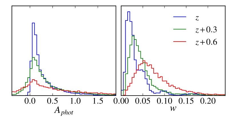
Figure 6.— Distributions of substructure statistics for the entire sample of simulated observations at different redshifts. (Left) The peak of $\rm{A_{phot}}$ distribution doesn’t move, for simulated observations at higher redshift. (Right) The peak of $w$ distribution shifts to higher values as the clusters are shifted to higher redshift.

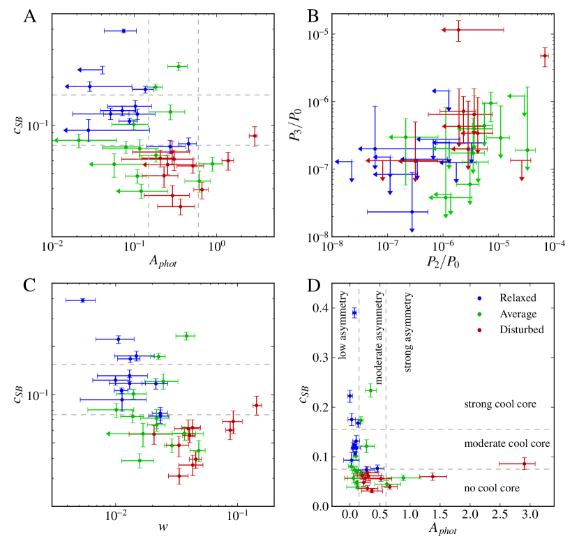
Figure 7.— A: Cluster classification by A_phot (substructure statistic introduced in this paper) and surface brightness concentration (c_SB; Santos et al., 2008). This classification scheme clearly separates relaxed, cool core clusters (high c_SB, low A_phot) from non-relaxed, disturbed systems (low c_SB, high A_phot). B: An alternative popular automatic classification scheme based on power ratios (Jeltema et al., 2005) – see text for details. Overall, the uncertainties are larger than in the asymmetry-concentration plane, and the clustering of same-type clusters is not as pronounced. C: Cluster classification using centroid shifts $w$ instead of $\rm{A_{phot}}$. Panel C achieves similarly good separation of relaxed and disturbed clusters, however the values of $w$ may be correlated with observational S/N as shown in Section 6.1. D: Same as A, but in linear coordinates. This plot emphasizes that there are no clusters that are both highly concentrated and “asymmetric”, consistent with the picture of cool cores representing a “relaxed” state that can be disrupted by cluster mergers. The horizontal dashed lines splitting the range of concentrations correspond to cool core categories as defined by Santos et al. (2008). The vertical dashed lines splitting the range of asymmetries correspond to asymmetry categories as defined here (low asymmetry: $\rm{A_{phot}}<0.15$; moderate asymmetry: $0.15<\rm{A_{phot}}<0.6$; strong asymmetry: $\rm{A_{phot}}>0.6$). In all panels, colors are assigned based on by-eye classification of “disturbance” (see text for details): blue - most relaxed, green - average, red - most disturbed. Where the corresponding values are consistent with zero they are plotted with arrows as their lower limits. Where they are negative, they are plotted with arrows at their upper limits. Values with negative upper limits are absent from the plots.

6.2. Asymmetry-concentration diagram

We propose a cluster classification scheme based on both concentration and asymmetry. Figure 7A shows the asymmetry-concentration diagram in logarithmic coordinates. The colors in Fig.7 are based on cluster “disturbance” as evaluated by-eye by a group of nine astronomers. Each participant was asked to score the disturbance of the clusters on the scale 1 to 3 (fractional values allowed), with 1 being least disturbed and 3 being most disturbed. We found that 11 of the clusters were unanimously ranked in the most disturbed half. We call this group of clusters “most disturbed”, and mark them in red in Figures 7, 8, and 9. Another 12 clusters were unanimously placed in the least disturbed half of the rankings. We call this group of clusters “relaxed” and mark them in blue. The remaining 13 clusters are “average” and marked in green.

The asymmetry-concentration diagram (Fig. 7A) shows a significantly better separation of clusters at different states of dynamical equilibrium (as assessed by human experts) than the competing scheme of cluster classification based on power ratios proposed by Jeltema et al. (2005) and presented in Fig. 7B. The other drawbacks of the power ratios classification scheme are that $\log P_{2}/P_{0}$ and $\log P_{3}/P_{0}$ correlate (correlation coefficient = 0.61) and that both $P_{2}/P_{0}$ and $P_{3}/P_{0}$ are often consistent with 0. Therefore, what we see in Fig. 7B is mostly noise, whereas most clusters in Fig. 7A show a significant detection of substructure as discussed above.

A similar separation of clusters at different states of dynamical equilibrium can be achieved using $w$ instead of $\rm{A_{phot}}$ as the substructure statistic (Fig. 7C), however $\rm{A_{phot}}$ is more stable and less biased for low S/N observations, as discussed above.

One can see that in Fig. 7A clusters avoid the upper right corner which confirms the standard assumption that concentrated or CC clusters are more regular. Fig. 7D, which is the same as Fig. 7A, but plotted in linear coordinates, shows this even better. It has a characteristic L-shape which implies that clusters are primarily either “concentrated” (upper part of the diagram) or “asymmetric” (right side) or “normal” (lower left corner).

In all the relevant panels of Fig. 7 we plot two dashed vertical lines as threshold values that separate low-, medium-, and strong-asymmetry clusters. The threshold values are $\rm{A_{phot}}>0.15$ and $\rm{A_{phot}}>0.6$. The horizontal dashed lines separate strong, moderate, and no cool cores as defined by Santos et al. (2008). The threshold values are $\rm{c_{SB}}>0.075$, and $\rm{c_{SB}}>0.155$.

The asymmetry-concentration classification scheme makes a clear separation between the radial and the angular structure. Concentration only probes the radial photon distribution, while asymmetry probes the angular photon distribution. We expect these to be uncorrelated, a point to which the data attest (correlation coefficient = -0.20). We show how asymmetry compares with power ratios and centroid shifts in Fig. 8. $\rm{A_{phot}}$ and $w$ are correlated strongly with correlation coefficient 0.87. This indicates that for high S/N data $\rm{A_{phot}}$ and $w$ agree well on which clusters are disturbed.

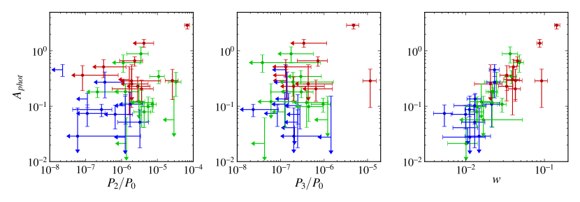
Figure 8.— Comparison of photon asymmetry, $\rm{A_{phot}}$, with power ratios, $P_{2}/P_{0}$ and $P_{3}/P_{0}$, and centroid shifts, $w$. Where power ratios are consistent with zero they are plotted with arrows as their lower limits. Where power ratios are negative, they are plotted with arrows at their upper limits. Power ratios with negative upper limits are absent from the plot. Colors are assigned based on by-eye classification of “disturbance”: blue - most relaxed, green - average, red - most disturbed (see text for details). There is no obvious correlation between $\rm{A_{phot}}$ and the other substructure parameters, with the exception that they all tend to agree on the most disturbed systems.

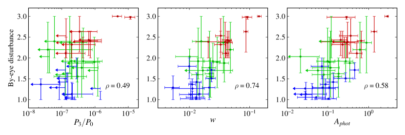
Figure 9.— Comparison of 3 substructure statistics with the average by-eye disturbance score as evaluated by a group of nine astronomers. The correlation coefficient between the by-eye score and the corresponding statistic is shown on the plots. The colors based on by-eye disturbance score in the same way as in Fig. 7 and 8.

6.3. Relative ranking of clusters by the amount of substructure, by-eye classification

In Fig. 9 we show how photon asymmetry, centroid shifts and $P_{3}/P_{0}$ power ratio compare to by-eye classification. We find that the photon asymmetry parameter correlates with the human “by-eye” ranks almost as strongly as centroid shifts, with a Spearman’s rank correlation coefficient of 0.71 for $\rm{A_{phot}}$, and 0.75 for $w$. Power ratio $P_{3}/P_{0}$, on the other hand, shows much lower correlation coefficient 0.47.

In Figures 10, 11, 12, we present three side-by-side comparisons of morphological indicators. In each figure the left panel shows the (same) X-ray images of galaxy clusters, ordered by increasing values of our photon asymmetry parameter. The right panel shows these same clusters, ranked by increasing centroid shifts, power ratio $P_{2}/P_{0}$, and by-eye disturbance, respectively. To produce by-eye ranking, we averaged the disturbance scores (1 to 3) obtained from all nine human experts. We then ranked clusters by average disturbance score.

7. Conclusions and future work

In this work, we introduced a new cluster substructure statistic – photon asymmetry ($\rm{A_{phot}}$), that measures the uniformity of the angular X-ray photon distribution in radial annuli. We compared photon asymmetry to two other measures of cluster morphology, power ratios (with a novel method for background correction) and centroid shifts, on the 400d cluster sample, and on simulated observations derived from it. Our focus was on performance of these substructure statistics in the low S/N regime, that is typical for observations of distant clusters. Our main conclusions are as follows

1. The angular resolution of a cluster observation is far more important than total counts for the ability to detect and quantify the substructure.

2. Both centroid shifts and photon asymmetry are significantly more sensitive to the amount of substructure than power ratios.

3. Both centroid shifts and photon asymmetry agree well with by-eye classification.

4. Centroid shifts are the best-performing substructure statistic in the low spatial resolution ($\theta\gtrsim 5^{\prime\prime}$) and background-dominated ($\sqrt{F_{bg}}\gtrsim F_{source}$) regimes.

5. Photon asymmetry is the best-performing substructure statistic in the low-counts regime.

6. Photon asymmetry is the most sensitive measure of the presence of substructure; 27 out of 36 clusters in the sample are classified by photon asymmetry as clusters with significant substructure (i.e., they are inconsistent with being axisymmetric), whereas the second best statistic, centroid shifts, finds significant substructure in only 21 out of 36 clusters.

7. Photon asymmetry is the only statistics that is insensitive to observational S/N below $\sim$ 1000 counts. Consequently, it is the only statistic suitable for comparison of clusters and cluster samples across large range of S/N, counts, backgrounds and redshifts. It is the best candidate for studying the influence of substructure on bias and scatter in scaling relations.

We also suggested using concentration (a measure of cool core strength) and asymmetry (which quantifies merging or disturbance) as the main parameters for cluster classification. We find that clusters can demonstrate either a high degree of concentration or asymmetry, but not both at the same time. It is possible to use centroid shifts instead of photon asymmetry as the measure of cluster disturbance, but asymmetry is preferable given its better stability with respect to observational S/N.

We are currently applying the photon asymmetry metric in a comparison of X-ray and SZ-selected cluster samples, to study the impact of morphology on cluster scaling relations, and to measure how morphology evolves with redshift.

As explained in Section 3, our method of calculating asymmetry includes 2 steps: calculating the asymmetry in an annulus and combining the asymmetries from several annuli. To measure the asymmetry in each annulus we use the statistical framework of testing whether a given sample is drawn from a given probability distribution. The sample in our case is the empirical angular photon distribution function $F_{N}$, and the given probability distribution is the true angular photon distribution function $G$ that would be produced by a perfectly circularly symmetric source. We note that $G$ is not trivial because of nonuniform detector illumination and various detector imperfections.

We define $F_{N}$ as the empirical cumulative angular distribution function of the photons in the $k$-th annulus:

$$F_{N}(x)=\frac{1}{N}\sum_{R_{in}^{k}<r_{i}<R_{out}^{k}}{\textbf{1}}\{\phi_{i}/2\pi\leq x\},$$ (1)

where ${\textbf{1}\{A\}}$ is the indicator function of event $A$ and $N$ is the number of counts within the annulus $R_{in}^{k}<r<R_{out}^{k}$. Also, for convenience we rescale the angular range $[0,2\pi)$ to $[0,1)$. Let $F$ be the true underlying distribution function for $F_{N}$, i.e $F$ is the limit of $F_{N}$ when $N\rightarrow\infty$.

Note that Kolmogorov-Smirnov, Cramer-von Mises and similar tests are usually used to check for the equality of 2 probability distributions. The values of these statistics give the probability of the null hypothesis (that the given sample is drawn from the given distribution), when compared to the null distribution. In our case, instead of checking whether $F_{N}$ is a realization of the known $F$ we need a measure of “distance” between $F$ and $G$ based on the measurement of $F_{N}$. In the following we show how one can use the value of Watson’s test (a modification of Cramer-von Mises test suitable for distributions defined on a circle as opposed to a segment) to quantify the distance between $F$ and $G$ based on the sample $F_{N}$.

In the following we will use the notation

$$\begin{gathered}U^{2}[F,G;dH]=\int\bigg{(}F(x)-G(x)-\int\Big{(}F(x)-G(x)\Big{)}dH(x)\bigg{)}^{2}dH(x),\end{gathered}$$ (2)

where $F$, $G$, and $H$ are arbitrary distribution functions defined on $[0,1]$, and all the integrals are taken over the same $[0,1]$ interval.

Using this notation, Watson’s statistic $U_{N}^{2}$ is simply

$$U_{N}^{2}=N\;U^{2}[F_{N},F;dF].$$ (3)

It can be viewed as a minimum of the $L_{2}$ distance between $F_{N}$ and $F$ over all possible points of origin on the circle (Watson, 1961):

$$U_{N}^{2}=\min_{\textrm{origin on the circle}}\int(F_{N}-F)^{2}dF.$$ (4)

In the limiting case $N\rightarrow\infty$, under the null hypothesis that the sample $\phi_{i}$ comes from the hypothesized distribution $F(x)$, the values of statistic $U_{\infty}^{2}=\lim_{N\rightarrow\infty}U_{N}^{2}$ have the same distribution as $K^{2}\pi^{-2}$, where $K$ is distributed according to Kolmogorov’s distribution:

$$\begin{gathered}\textrm{Prob}\{U_{\infty}^{2}<x\}=\textrm{Prob}\{K<\pi\sqrt{x}\}=1-2\sum_{k=1}^{\infty}(-1)^{k-1}e^{-2k^{2}\pi^{2}x^{2}}.\end{gathered}$$ (5)

We won’t need the exact form of this limiting distribution, but we need to know its mean which can be derived from known moments of Kolmogorov’s distribution:

$$\langle U_{\infty}^{2}\rangle=\frac{\langle K^{2}\rangle}{\pi^{2}}=\frac{1}{12}.$$ (6)

It may be shown (Watson, 1961) that given a discrete sample $x_{1},x_{2},\cdots,x_{N}$ hypothetically distributed according to $F(x)$, the statistic can be computed as

$$U_{N}^{2}=\frac{1}{12N}+\sum_{i=0}^{N-1}\left(\frac{2i+1}{2N}-F_{i}\right)^{2}-N\left(\frac{1}{2}-\frac{1}{N}\sum_{i=0}^{N-1}F_{i}\right)^{2},$$ (7)

where $F_{i}=F(x_{i})$.

Now let’s apply Watson’s test statistic to the empirical distribution function $F_{N}$ and an arbitrary distribution function $G$ to which we need to compute a distance (in our method $G$ is the distribution function that represents a circularly symmetric source)

$$W_{N}^{2}=NU^{2}[F_{N},G;dG].$$ (8)

Integrating by parts one can show that

$$U^{2}[F_{N},G;dG]=U^{2}[F_{N},G;dF_{N}].$$ (9)

Now we will replace $dF_{N}$ with $dF$ in the right hand side of (9). While it is evident (Doob, 1949) that as $N\rightarrow\infty$

$$U^{2}[F_{N},G;dF_{N}]-U^{2}[F_{N},G;dF]=R_{N}^{2}\rightarrow 0\textrm{ in probability,}$$ (10)

the merit of this approximation and the rate of convergence are discussed below.

$U^{2}[F_{N},G;dF]$ can be transformed in the following way

$$\begin{gathered}U^{2}[F_{N},G;dF]=\int\bigg{[}\Big{(}F_{N}-F-\int(F_{N}-F)dF\Big{)}+\Big{(}F-G-\int(F-G)dF\Big{)}\bigg{]}^{2}dF\\ =U^{2}[F_{N},F;dF]+\int\Big{(}F_{N}-F-\int(F_{N}-F)dF\Big{)}\cdot\Big{(}F-G-\int(F-G)dF\Big{)}dF+U^{2}[F,G;dF]\end{gathered}$$ (11)

The first term, $U^{2}[F_{N},F;dF]$ is distributed according to Kolmogorov’s distribution and its mean is $\frac{1}{12}$ (see Eq. (6)).

The second term,

$$V=\int(F_{N}-F-\Delta)g(x)dx,\;\;g(x)=(F-G-\int(F-G)dF)F^{\prime}(x)$$ (12)

has zero mean, because it is a sum of integrals of a function which has zero expectation value at any point on the segment

$$\langle F_{N}(x)-F(x)\rangle=0\;\;\forall x:0<x<1$$ (13)

with bounded functions $g(x)$ and $\int g(x)dx=const$.

The third term is the desired distance $d$ between $F$ and $G$.

Combining (8), (10) and (11) we find the following estimator $\hat{d}_{N}$ of $d$

$$\hat{d}_{N}=\frac{W_{N}^{2}}{N}-\frac{1}{12N}.$$ (14)

This estimator is biased by the average value of $R_{N}^{2}$.

$$\langle\hat{d}_{N}-d\rangle=\langle U^{2}[F_{N},G;dF_{N}]-U^{2}[F_{N},G;dF]\rangle=\langle R_{N}^{2}\rangle$$ (15)

We were not able to obtain an analytic bound on $R_{N}^{2}$ and its $N$-dependence. Judging by the form of (10), $R_{N}^{2}$ should be of order $1/\sqrt{N}$. Considering this asymptotic behavior of $R_{N}^{2}$, our wish to explicitly correct for “smaller” bias $1/12N$ may look strange. The reason for this explicit correction is that $1/12N$ is bigger than $R_{N}^{2}$ for relevant values of $N$ ($N<10^{3}$). We confirmed this statement by multiple numerical experiments with various distribution functions $F$ and $G$. As $N$ reaches higher values ($N\sim 10^{4}$) $\langle R_{N}^{2}\rangle$ can become greater than $1/12N$, but both terms tend to zero with increasing $N$.

Now we need to take into account that the acquired light comes both from the cluster and the background. We model the counts distribution function $F$ as a weighted sum of cluster emission $F_{Cl}$ and a uniform background $G$

$$F=\alpha F_{Cl}+\beta G,\quad\alpha+\beta=1,\quad\alpha=C/N,$$ (16)

where $C$ is the number of cluster counts, and $N$ is the total number of counts in the given annulus. Then we obtain

$$d=\int\Big{(}F-G-\int(F-G)dG\Big{)}^{2}dG=\alpha^{2}\int\Big{(}F_{Cl}-G-\int(F_{Cl}-G)dG\Big{)}^{2}dG=\alpha^{2}d_{Cl}$$ (17)

Now, using (14) we see that

$$d_{N,Cl}=\frac{N}{C^{2}}\Big{(}W_{N}^{2}-\frac{1}{12}\Big{)}$$ (18)

is our estimator of the distance between the observed photon distribution function $F_{N}$ and the underlying cluster emission distribution function $F_{Cl}$.

The sum of distances $d_{Cl}^{(k)}$ in 4 annuli, where $k$ numbers the annuli, weighted by the estimated number of cluster counts in these annuli $C_{k}$, and multiplied by 100 gives photon asymmetry:

$$A_{phot}=100\sum_{k=1}^{4}C_{k}d_{N_{k},Cl}^{(k)}/\sum_{k=1}^{4}C_{k}.$$ (19)

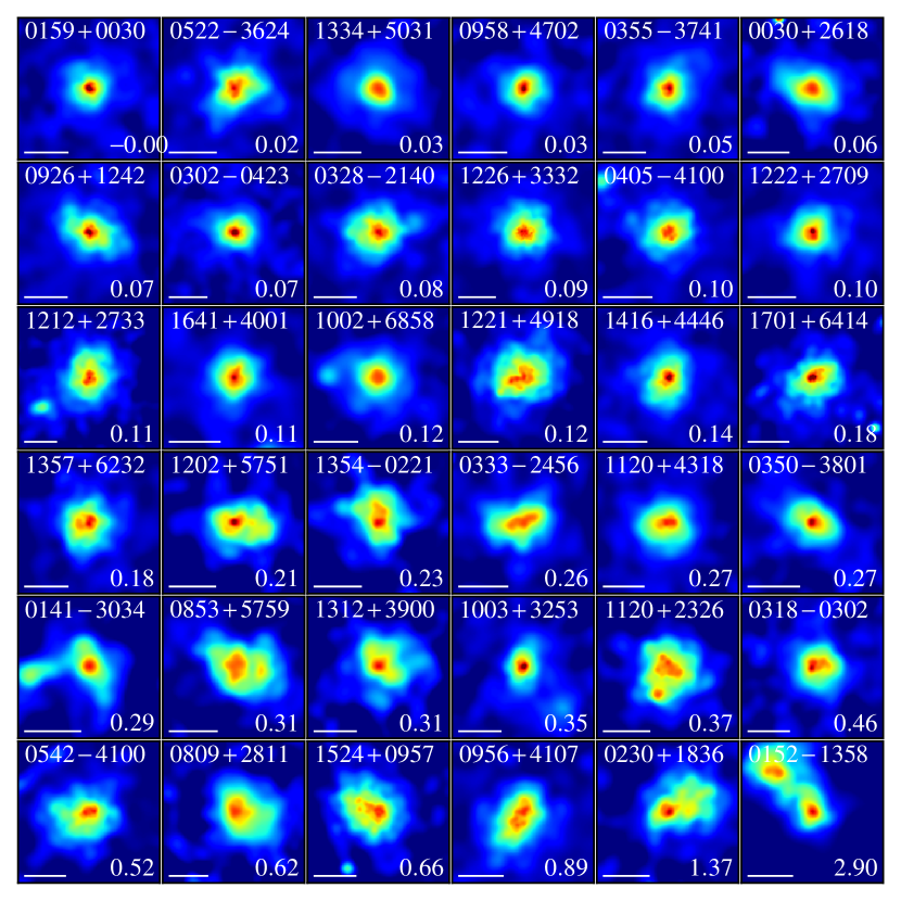
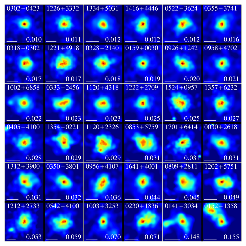
Figure 10.— Clusters sorted by asymmetry (left) and centroid shifts (right). The value of the substrucure statistics increases top-to-bottom, left-to-right in both plots. Cluster name is in upper right corner, the value of the statistic is in the upper left corner. The names of the clusters are identical to those used in Vikhlinin et al. (2009a). Left plot. Clusters sorted by the value of asymmetry - the new substructure measure which is presented in this paper. Right plot. Clusters sorted by the value of centroid shifts.

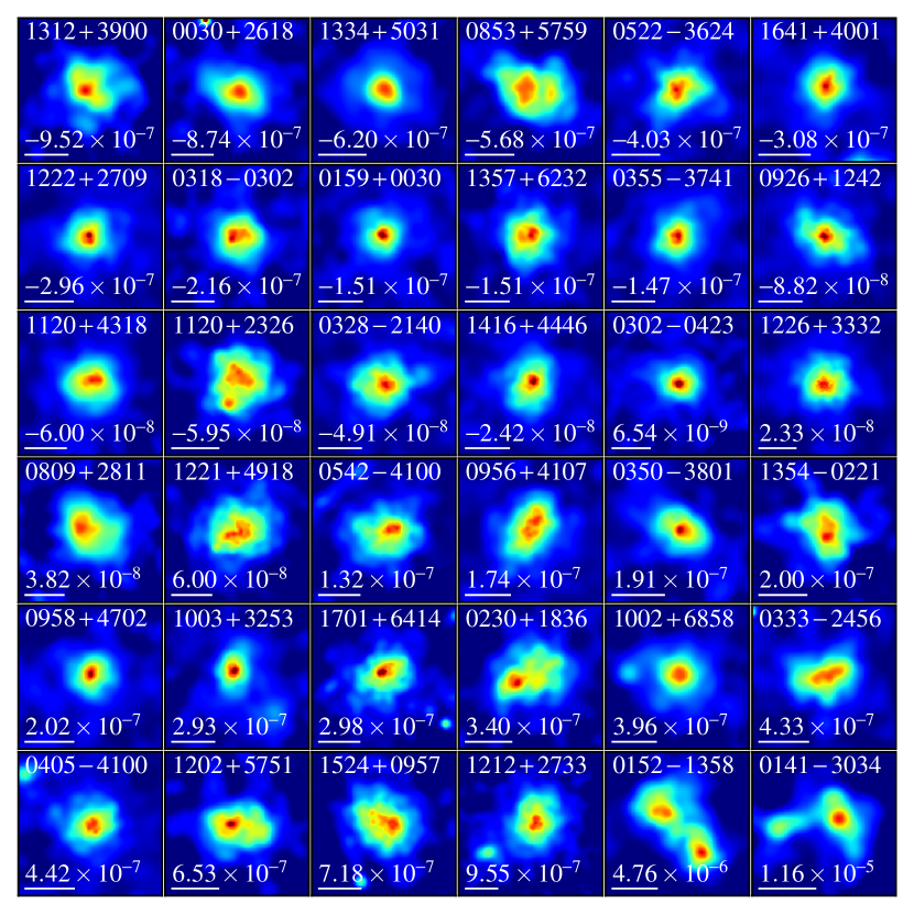
Figure 11.— Clusters sorted by asymmetry (left) and power ratios $P_{3}/P_{0}$ (right). The value of the substrucure statistics increases top-to-bottom, left-to-right in both plots. Cluster name is in upper right corner, the value of the statistic is in the upper left corner The names of the clusters are identical to those used in Vikhlinin et al. (2009a). Left plot. Clusters sorted by the value of asymmetry - the new substructure measure which is presented in this paper. Right plot. Clusters sorted by the value of $P_{3}/P_{0}$. White circle is the aperture used for calculating power ratio ($R_{500}$).

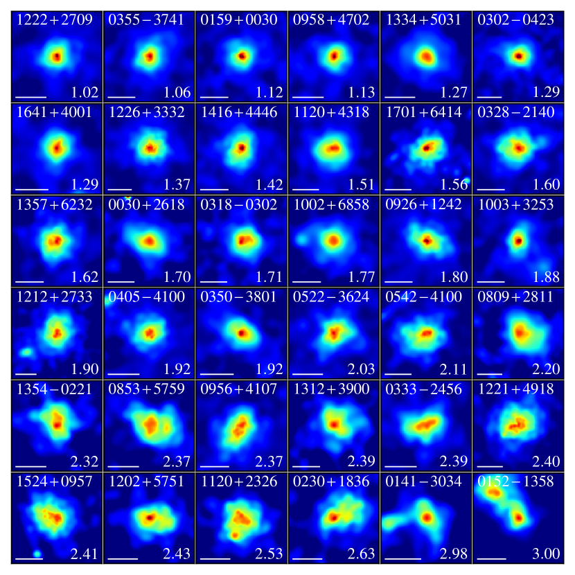
Figure 12.— Clusters sorted by asymmetry (left) and ”by-eye” level of disturbance (right). The value of the substrucure statistics increases top-to-bottom, left-to-right in both plots. Cluster name is in upper right corner, the value of the statistic is in the upper left corner The names of the clusters are identical to those used in Vikhlinin et al. (2009a). Left plot. Clusters sorted by the value of asymmetry - the new substructure measure which is presented in this paper. Right plot. Clusters sorted by the average value of their ”disturbness” evaluated by 4 numan experts.

References

- Allen et al. (2011) Allen, S. W., Evrard, A. E., & Mantz, A. B. 2011, ARA&A, 49, 409
- Andrade-Santos et al. (2012) Andrade-Santos, F., Lima Neto, G. B., & Laganá, T. F. 2012, ApJ, 746, 139
- Blanton et al. (2011) Blanton, E. L., Randall, S. W., Clarke, T. E., Sarazin, C. L., McNamara, B. R., Douglass, E. M., & McDonald, M. 2011, ApJ, 737, 99
- Böhringer et al. (2010) Böhringer, H., Pratt, G. W., Arnaud, M., Borgani, S., Croston, J. H., Ponman, T. J., Ameglio, S., Temple, R. F., & Dolag, K. 2010, A&A, 514, A32
- Böhringer et al. (2000) Böhringer, H., Soucail, G., Mellier, Y., Ikebe, Y., & Schuecker, P. 2000, A&A, 353, 124
- Böhringer & Werner (2010) Böhringer, H., & Werner, N. 2010, A&A Rev., 18, 127
- Buote (2002) Buote, D. A. 2002, in Astrophysics and Space Science Library, Vol. 272, Merging Processes in Galaxy Clusters, ed. L. Feretti, I. M. Gioia, & G. Giovannini, 79–107
- Buote & Tsai (1995) Buote, D. A., & Tsai, J. C. 1995, ApJ, 452, 522
- Buote & Tsai (1996) —. 1996, ApJ, 458, 27
- Burenin et al. (2007) Burenin, R. A., Vikhlinin, A., Hornstrup, A., Ebeling, H., Quintana, H., & Mescheryakov, A. 2007, ApJS, 172, 561
- Cassano et al. (2010) Cassano, R., Ettori, S., Giacintucci, S., Brunetti, G., Markevitch, M., Venturi, T., & Gitti, M. 2010, ApJ, 721, L82
- Conselice (2003) Conselice, C. J. 2003, ApJS, 147, 1
- Doob (1949) Doob, J. L. 1949, The Annals of Mathematical Statistics, 20, 393
- Ebeling et al. (2006) Ebeling, H., White, D. A., & Rangarajan, F. V. N. 2006, MNRAS, 368, 65
- Fabian et al. (1994) Fabian, A. C., Crawford, C. S., Edge, A. C., & Mushotzky, R. F. 1994, MNRAS, 267, 779
- Ferrari et al. (2008) Ferrari, C., Govoni, F., Schindler, S., Bykov, A. M., & Rephaeli, Y. 2008, Space Sci. Rev., 134, 93
- Fruscione et al. (2006) Fruscione, A., McDowell, J. C., Allen, G. E., Brickhouse, N. S., Burke, D. J., Davis, J. E., Durham, N., Elvis, M., Galle, E. C., Harris, D. E., Huenemoerder, D. P., Houck, J. C., Ishibashi, B., Karovska, M., Nicastro, F., Noble, M. S., Nowak, M. A., Primini, F. A., Siemiginowska, A., Smith, R. K., & Wise, M. 2006, in Society of Photo-Optical Instrumentation Engineers (SPIE) Conference Series, Vol. 6270, Society of Photo-Optical Instrumentation Engineers (SPIE) Conference Series
- Hallman & Jeltema (2011) Hallman, E. J., & Jeltema, T. E. 2011, MNRAS, 418, 2467
- Hallman et al. (2010) Hallman, E. J., Skillman, S. W., Jeltema, T. E., Smith, B. D., O’Shea, B. W., Burns, J. O., & Norman, M. L. 2010, ApJ, 725, 1053
- Hart (2008) Hart, B. C. 2008, PhD thesis, Proquest Dissertations And Theses 2008. Section 0030, Part 0538 163 pages; [Ph.D. dissertation].United States – California: University of California, Irvine; 2008. Publication Number: AAT 3296261. Source: DAI-B 69/01, Jul 2008
- Hogg et al. (2002) Hogg, D. W., Baldry, I. K., Blanton, M. R., & Eisenstein, D. J. 2002, ArXiv Astrophysics e-prints
- Hudson et al. (2010) Hudson, D. S., Mittal, R., Reiprich, T. H., Nulsen, P. E. J., Andernach, H., & Sarazin, C. L. 2010, A&A, 513, A37
- Jeltema et al. (2005) Jeltema, T. E., Canizares, C. R., Bautz, M. W., & Buote, D. A. 2005, ApJ, 624, 606
- Kay et al. (2008) Kay, S. T., Powell, L. C., Liddle, A. R., & Thomas, P. A. 2008, MNRAS, 386, 2110
- Markevitch & Vikhlinin (2007) Markevitch, M., & Vikhlinin, A. 2007, Phys. Rep., 443, 1
- McDonald et al. (2013) McDonald, M., Benson, B. A., Vikhlinin, A., Stalder, B., Bleem, L. E., Lin, H. W., Aird, K. A., Ashby, M. L. N., Bautz, M. W., Bayliss, M., Bocquet, S., Brodwin, M., Carlstrom, J. E., Chang, C. L., Cho, H. M., Clocchiatti, A., Crawford, T. M., Crites, A. T., de Haan, T., Desai, S., Dobbs, M. A., Dudley, J. P., Foley, R. J., Forman, W. R., George, E. M., Gettings, D., Gladders, M. D., Gonzalez, A. H., Halverson, N. W., High, F. W., Holder, G. P., Holzapfel, W. L., Hoover, S., Hrubes, J. D., Jones, C., Joy, M., Keisler, R., Knox, L., Lee, A. T., Leitch, E. M., Liu, J., Lueker, M., Luong-Van, D., Mantz, A., Marrone, D. P., McMahon, J. J., Mehl, J., Meyer, S. S., Miller, E. D., Mocanu, L., Mohr, J. J., Montroy, T. E., Murray, S. S., Nurgaliev, D., Padin, S., Plagge, T., Pryke, C., Reichardt, C. L., Rest, A., Ruel, J., Ruhl, J. E., Saliwanchik, B. R., Saro, A., Sayre, J. T., Schaffer, K. K., Shirokoff, E., Song, J., Suhada, R., Spieler, H. G., Stanford, S. A., Staniszewski, Z., Stark, A. A., Story, K., van Engelen, A., Vanderlinde, K., Vieira, J. D., Williamson, R., Zahn, O., & Zenteno, A. 2013, ArXiv e-prints
- McNamara & Nulsen (2007) McNamara, B. R., & Nulsen, P. E. J. 2007, ARA&A, 45, 117
- Mohr et al. (1995) Mohr, J. J., Evrard, A. E., Fabricant, D. G., & Geller, M. J. 1995, ApJ, 447, 8
- Mohr et al. (1993) Mohr, J. J., Fabricant, D. G., & Geller, M. J. 1993, ApJ, 413, 492
- Mohr et al. (1999) Mohr, J. J., Mathiesen, B., & Evrard, A. E. 1999, ApJ, 517, 627
- Neumann & Bohringer (1997) Neumann, D. M., & Bohringer, H. 1997, MNRAS, 289, 123
- O’Hara et al. (2006) O’Hara, T. B., Mohr, J. J., Bialek, J. J., & Evrard, A. E. 2006, ApJ, 639, 64
- Peterson & Fabian (2006) Peterson, J. R., & Fabian, A. C. 2006, Phys. Rep., 427, 1
- Pinkney et al. (1996) Pinkney, J., Roettiger, K., Burns, J. O., & Bird, C. M. 1996, ApJS, 104, 1
- Poole et al. (2006) Poole, G. B., Fardal, M. A., Babul, A., McCarthy, I. G., Quinn, T., & Wadsley, J. 2006, MNRAS, 373, 881
- Rasia (2013) Rasia, E. 2013, The Astronomical Review, 8, 010000
- Sanderson et al. (2009) Sanderson, A. J. R., Edge, A. C., & Smith, G. P. 2009, MNRAS, 398, 1698
- Santos et al. (2008) Santos, J. S., Rosati, P., Tozzi, P., Böhringer, H., Ettori, S., & Bignamini, A. 2008, A&A, 483, 35
- Santos et al. (2010) Santos, J. S., Tozzi, P., Rosati, P., & Böhringer, H. 2010, A&A, 521, A64
- Semler et al. (2012) Semler, D. R., Šuhada, R., Aird, K. A., Ashby, M. L. N., Bautz, M., Bayliss, M., Bazin, G., Bocquet, S., Benson, B. A., Bleem, L. E., Brodwin, M., Carlstrom, J. E., Chang, C. L., Cho, H. M., Clocchiatti, A., Crawford, T. M., Crites, A. T., de Haan, T., Desai, S., Dobbs, M. A., Dudley, J. P., Foley, R. J., George, E. M., Gladders, M. D., Gonzalez, A. H., Halverson, N. W., Harrington, N. L., High, F. W., Holder, G. P., Holzapfel, W. L., Hoover, S., Hrubes, J. D., Jones, C., Joy, M., Keisler, R., Knox, L., Lee, A. T., Leitch, E. M., Liu, J., Lueker, M., Luong-Van, D., Mantz, A., Marrone, D. P., McDonald, M., McMahon, J. J., Mehl, J., Meyer, S. S., Mocanu, L., Mohr, J. J., Montroy, T. E., Murray, S. S., Natoli, T., Padin, S., Plagge, T., Pryke, C., Reichardt, C. L., Rest, A., Ruel, J., Ruhl, J. E., Saliwanchik, B. R., Saro, A., Sayre, J. T., Schaffer, K. K., Shaw, L., Shirokoff, E., Song, J., Spieler, H. G., Stalder, B., Staniszewski, Z., Stark, A. A., Story, K., Stubbs, C. W., van Engelen, A., Vanderlinde, K., Vieira, J. D., Vikhlinin, A., Williamson, R., Zahn, O., & Zenteno, A. 2012, ApJ, 761, 183
- Vazza et al. (2011) Vazza, F., Brunetti, G., Gheller, C., Brunino, R., & Brüggen, M. 2011, A&A, 529, A17
- Ventimiglia et al. (2008) Ventimiglia, D. A., Voit, G. M., Donahue, M., & Ameglio, S. 2008, ApJ, 685, 118
- Vikhlinin et al. (2009a) Vikhlinin, A., Burenin, R. A., Ebeling, H., Forman, W. R., Hornstrup, A., Jones, C., Kravtsov, A. V., Murray, S. S., Nagai, D., Quintana, H., & Voevodkin, A. 2009a, ApJ, 692, 1033
- Vikhlinin et al. (2009b) Vikhlinin, A., Kravtsov, A. V., Burenin, R. A., Ebeling, H., Forman, W. R., Hornstrup, A., Jones, C., Murray, S. S., Nagai, D., Quintana, H., & Voevodkin, A. 2009b, ApJ, 692, 1060
- Voit (2011) Voit, G. M. 2011, ApJ, 740, 28
- Watson (1961) Watson, G. 1961, Biometrika, 48, 109
- Weißmann et al. (2013) Weißmann, A., Böhringer, H., Šuhada, R., & Ameglio, S. 2013, A&A, 549, A19