Dynamical regimes of dissipative quantum systems

Abstract

We reveal several distinct regimes of the relaxation dynamics of a small quantum system coupled to an environment within the plane of the dissipation strength and the reservoir temperature. This is achieved by discriminating between coherent dynamics with damped oscillatory behavior on all time scales, partially coherent behavior being nonmonotonic at intermediate times but monotonic at large ones, and purely monotonic incoherent decay. Surprisingly, elevated temperature can render the system ‘more coherent’ by inducing a transition from the partially coherent to the coherent regime. This provides a refined view on the relaxation dynamics of open quantum systems.

When studying the relaxation dynamics of a small quantum system coupled to a dissipative environment at low temperatures $T$ one usually encounters coherent dynamics which is damped oscillatory at weak coupling and monotonic incoherent dynamics at stronger ones. The best studied example comprising this generic physics is the ohmic spin boson model (SBM). Leggett87 ; Weiss12 This model can be visualized by a spin-$\nicefrac{{1}}{{2}}$ degree of freedom with tunneling between the up and down states as well as coupling to a bosonic reservoir. Nonuniversal effects which depend on the details of the reservoir band dominate the behavior at short times $t$ up to $\omega_{\rm c}^{-1}$ set by the inverse band width. We are interested in the universal aspects and exclusively consider the limit in which $\omega_{\rm c}$ is much larger than any other energy scale of the problem (scaling limit). It is well established that in the unbiased case (vanishing Zeeman field) and for coupling $\nicefrac{{1}}{{2}}<\alpha<1$ of the spin and the reservoir the expectation value $P(t)=\left<\sigma_{z}(t)\right>$ monotonically approaches zero, i.e. the dynamics is incoherent. At large $t$ it can be described by an exponentially decaying function, possibly with subdominant corrections. Egger97 ; Kennes13a ; Wang08 ; Kashuba13a ; Kashuba13b In contrast, for $\alpha\ll 1$ and small $T$, $P(t)$ is a damped oscillatory function (coherent dynamics). Leggett87 ; Weiss12 ; Wang08 ; Anders06 ; Orth10A ; Orth13 Even at small $\alpha$ raising $T$ will eventually drive the system into the incoherent regime. Garg85 ; Weiss86 ; Leggett87 ; Weiss12 ; Orth10A ; Orth13

We show that the classification into coherent and incoherent behavior—with the definition of ‘coherence’ given above—must be refined and provide a more detailed understanding of the dynamics realized in the $\alpha$–$T$ plane by discriminating between intermediate and long times.Kennes13a ; Kashuba13b Our insights form an improved basis for future studies on the relaxation dynamics of dissipative quantum systems as investigated in condensed matter physics, quantum optics, physical chemistry, and quantum information science. Leggett87 ; Weiss12

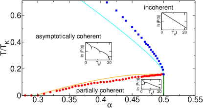
Figure 1: (Color online) Diagram showing the extend of the incoherent, asymptotically, and partially coherent sectors. The critical temperatures $T_{\rm c1}$ (lower branch) and $T_{\rm c2}$ (upper branch) obtained from the numerical solution of the RTRG equations (4) are shown as circles; solid lines correspond to the approximatations Eqs. (7) (lower) and (8) (upper). The insets exemplify the time evolution of the spin expectation value $P(t)$ in the different regimes for $\alpha=0.45$ and $T/T_{\rm K}=0.01$ (partially coherent), $0.3$ (asymptotically coherent), $0.59$ (incoherent), with the Kondo scale $T_{\rm K}$.

Our results are summarized in Fig. 1 showing the extend of the different regimes of distinct dynamical behavior in the $\alpha$–$T$ plane. For $0<\nicefrac{{1}}{{2}}-\alpha\ll 1$ and sufficiently small $T$ we find a regime in which $P(t)$ is nonmonotonic (‘oscillatory’) on intermediate times, but monotonic on large ones. In the following we denote this the partially coherent regime. It must be distinguished from the asymptotically coherent one encountered at small $\alpha$ and $T$,Leggett87 ; Weiss12 ; Garg85 ; Weiss86 in which $P(t)$ shows damped oscillatory behavior on all time scales. We find a transition line between the partially and the asymptotically coherent regimes when raising $T$, which constitutes the central result of our work. It implies that for $0<\nicefrac{{1}}{{2}}-\alpha\ll 1$ the dynamics is more coherent at elevated temperatures than at low ones, which is rather counterintuitive. At even larger $T$, $P(t)$ will eventually become purely monotonic and the dynamics is incoherent. For $\nicefrac{{1}}{{2}}<\alpha<1$ it is incoherent for all $T$.

At $T=0$ the appearance of the partially coherent regime in between the more standard asymptotically coherent and incoherent ones can be shown analytically.Egger97 ; Kennes13a ; Kashuba13b For $T>0$ our numerical results for $P(t)$ obtained by two complementary renormalization group (RG) approaches—the real-time RG (RTRG) Schoeller09 and the functional RG (FRG) Metzner12 —indicate the transition between the partially and the asymptotically coherent regimes when increasing $T$. In Fig. 2 we show $|P(t)|$ for different $T$ at fixed $\alpha$ close to $\nicefrac{{1}}{{2}}$ (see also the insets of Fig. 1). At $T=0$ one starts out in the partially coherent regime with $P(t)$ having a single zero (dip in a linear-logarithmic plot of $|P(t)|$). Increasing $T$, more zeros appear signalling the transition to the asymptotically coherent regime; next, the distance between the zeros increases and eventually all of them disappear when entering the incoherent one.

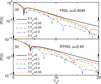
Figure 2: (Color online) Time dependence of the spin expectation value $|P(t)|$ on a linear-logarithmic scale [(a) FRG, (b) RTRG]. Both approaches capture the transition from partially coherent to asymptotically coherent to incoherent dynamics when raising $T$.

A more detailed understanding can be obtained from studying the Laplace transform $\Pi_{1}(E)=\int_{0}^{\infty}dt\,e^{iEt}P(t)$ of the spin expectation value in the lower half of the complex $E$-plane. This also allows to precisely determine the transition termperatures. Our RTRG approach is set up in Liouville-Laplace space Pletyukhov12 ; Kennes13a ; Kashuba13b ; Kashuba13a and $\Pi_{1}(E)$ can be accessed directly through the numerical integration of the RG flow equations. The relaxation dynamics is determined by the nonanalyticities of the propagator $\Pi_{1}(E)$ at $z_{n}\in{\mathbb{C}}$. Each yields a separate contribution to $P(t)$ of the form $\sim\exp{(iz_{n}t)}$, where the frequency and decay rate are determined by $\mbox{Re}\,z_{n}$ and $\mbox{Im}\,z_{n}$, respectively. For branch cuts the exponential decay is accompanied by weakly $t$-dependent corrections. Egger97 ; Kennes13a ; Kashuba13b ; Wang08 ; Kashuba13a The nonanalyticity closest to the real axis dominates the dynamics at large $t$. Figure 3 highlights the singularities and branch cuts (dark features) of $\Pi_{1}(E)$ for $\alpha=0.45$ and different $T$. For $0<\nicefrac{{1}}{{2}}-\alpha\ll 1$ and $T=0$, $\Pi_{1}(E)$ has a pair of poles with nonvanishing real parts of equal absolute value [damped oscillations of $P(t)$] as well as a branch cut on the imaginary axis [monotonic decay of $P(t)$]. The distance of the start of the branch cut to the real axis is smaller than the distance between the latter and the poles. Thus for large $t$ the branch cut term prevails giving rise to partially coherent relaxation dynamics.Kennes13a ; Kashuba13b For $T>0$ the branch cut disintegrates into singularities, Garg85 ; Weiss86 as can be seen in Fig. 3(a). Raising $T$ these move down while the imaginary part of the finite frequency poles barely changes, see Fig. 3(b). When the top zero frequency singularity passes the level of the pole pair $T_{\rm c1}(\alpha)$ is reached and the system undergoes a transition into the asymptotically coherent regime, see Fig. 3(c). Further incerasing $T$ the oscillation frequency decreases as the pair of poles starts to move inwards, while the singularities on the imaginary axis continue to move down and leave the frame shown in Fig. 3, see Fig. 3(d). The frequency vanishes when the pole pair hits the imaginary axis at $T_{\rm c2}(\alpha)$, indicating the transition from asymptotically coherent to incoherent dynamics, see Fig. 3(e). At further increasing $T$ two singularities move in opposite directions along the imaginary axis such that the one moving up approaches the decay rate of $\alpha=\nicefrac{{1}}{{2}}$ for $T\to\infty$, see Fig. 3(f). The $T_{\rm c1/2}$ obtained by such an analysis varying $T$ and $\alpha$ are shown as circles in Fig. 1. The additional finite frequency features (black circles with gray tails) visible in Figs. 3(b) and (c) are artifacts of our leading order (in $\nicefrac{{1}}{{2}}-\alpha$) approximation (see below).

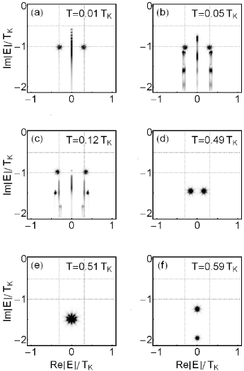
Figure 3: Nonanalytical features of the propagator $\Pi_{1}(E)$ at coupling $\alpha=0.45$. Density plots of $|\partial_{\mathrm{Im}\,E}\mathrm{Re}\,\Pi_{1}+\partial_{\mathrm{Re}\,E}\mathrm{Im}\,\Pi_{1}|$ as a function of the complex variable $E$ are shown. Dashed horizontal lines indicate the zero temperature decay rates for the poles $T_{\rm K}$ and branching point $T_{\rm K}/2$. Vertical ones indicate the frequency $\pm\Omega$ of the poles at $T=0$ ($\Omega\approx\pi gT_{\rm K}$ .Egger97 ; Kennes13a ; Kashuba13b ; Lesage98 )

Model and setup—The unbiased SBM is given by the Hamiltonian

$$H=-\frac{\Delta}{2}\sigma_{x}+\sum_{k}\omega_{k}b_{k}^{\dagger}b_{k}-\sum_{k}\frac{\lambda_{k}}{2}\sigma_{z}\left(b_{k}^{\dagger}+b_{k}\right),$$ (1)

with the Pauli matrices $\sigma_{\nu}$, $\nu=x,z$, bosonic ladder operators $b_{k}^{({\dagger})}$, tunneling amplitude $\Delta$, reservoir dispersion $\omega_{k}$, and coupling $\lambda_{k}$. The spin-boson coupling is characterized by a spectral density $J(\omega)=\sum_{k}\lambda_{k}^{2}\delta(\omega-\omega_{k})$. Its $\omega$ dependence is set by the details of the microscopic model underlying the SBM.Leggett87 We focus on the ohmic case with $J(\omega)=2\alpha\omega\Theta(\omega_{\rm c}-\omega)$, $\alpha\geq 0$; $\omega_{\rm c}$ and $\Delta$ only enter in the combination $T_{\rm K}=\Delta\left(\Delta/\omega_{\rm c}\right)^{\alpha/(1-\alpha)}$ defining the emergent Kondo scale.Leggett87 ; Weiss12

We prepare the system as the product of the spin-up state (in $z$-direction) and the canonical density matrix ($T>0$) for the reservoir. At time $t=0$ the coupling between the spin and the bosons is switched on and the relaxation sets in. For $\alpha<1$ and infinitely large times a steady state with $\lim_{t\to\infty}P(t)=0$ is reached. Here we do not consider the quantum phase transition to the localized regime with $\lim_{t\to\infty}P(t)\neq 0$ at $\alpha=1$.Leggett87 ; Weiss12 We considered other initial density matrices and verified that the classification of the dynamics is not affected by the particular choice of the $t=0$ state.

Investigating the most interesting regime $|\nicefrac{{1}}{{2}}-\alpha|\ll 1$ we do not study the SBM but rather employ the mapping to the interacting resonant level model (IRLM).Leggett87 ; Weiss12 ; Kashuba13b Within the IRLM $\alpha=\nicefrac{{1}}{{2}}$ corresponds to the noninteracting limit. Our RG methods provide controlled access to the relaxation dynamics around this exactly solvable point. For the FRG this was earlier shown for $T\geq 0$.Kennes12 ; Kennes13b In fact, the RG flow equations for the one-particle irreducible vertex functions of Ref. Kennes13b, can directly be used to numerically compute $P(t)$. For $T=0$ RTRG equations were derived in Refs. Kennes13a, ; Kashuba13b, .

RTRG for finite temperatures—We next discuss how to extend the RTRG approach to $T>0$ and describe the steps to derive analytical expressions for $T_{\rm c1/2}(\alpha)$. Readers interested in results only can skip this part.

In the RTRG approach one aims at the reduced density matrix of the spin.Schoeller09 ; Pletyukhov12 Integrating out the reservoirs’ degrees of freedom at $T>0$ leads to a summation over Matsubara frequencies $\omega_{m}=\pi T(2m+1)$. The RG equations for the relaxation rates $\Gamma_{1/2}$ derived in Refs. Kennes13a, ; Kashuba13b, for $T=0$ thus change to

$$\frac{d\Gamma_{1/2}(E)}{dE} = ig\Gamma_{1}(E)\,2\pi T\sum_{m=0}^{\infty}\Bigl{[}\Pi_{2/1}\bigl{(}E+i\omega_{m}\bigr{)}\Bigr{]}^{2},$$ (2)

$$\Pi_{n}(E) = i\left[E+i\Gamma_{n}(E)/n\right]^{-1},\;\;n=1,2$$ (3)

where $g=1-2\alpha$ is the small parameter and the initial conditions read $\Gamma_{1/2}(i\omega_{\rm c})=\Delta^{2}/\omega_{\rm c}$. To perform the Matsubara sum to order $g$ we neglect the $E$-dependence of $\Gamma_{1/2}$ in $\Pi_{2/1}$, which yields

$$\frac{d\Gamma_{1/2}(E)}{dE}=ig\frac{\Gamma_{1}(E)}{2\pi T}\psi^{\prime}\left(\frac{1}{2}+\frac{1}{2\pi T\Pi_{2/1}(E)}\right),$$ (4)

where $\psi^{\prime}(z)$ is the trigamma function. This set of equations was solved numerically to obtain Fig. 3 and, after an additional (numerical) Laplace back transform, Fig. 2(b).

The right hand side of the differential equation (4) contains a series of second order poles, which after integration turn into essential singularities of the propagator $\Pi_{1}$ at $z_{n}$. They result from the disintegration of the branch cut of $\Gamma_{1}(E)$ found at $T=0$ Egger97 ; Kennes13a ; Kashuba13b and are located on the imaginary axis Garg85 ; Weiss86 [see Fig. 3(a)]; their mutual distance is $2\pi T[1+{\mathcal{O}}(g)]$. Close to those singularities we find $\Pi_{1}\propto e^{-g/(E-z_{n})}$. The finite frequency branch cuts (black circles with gray tails) of Figs. 3(b) and (c) are artifacts of the lowest order truncation. In the full diagrammatic series underlying the RTRG approach Schoeller09 no integrals over the reservoirs excitation frequencies appear for $T>0$, but only summations over $\omega_{m}$. Therefore, branch cuts are excluded. The contributions of the artificial nonanalyticities to $P(t)$, however, are of order $g^{2}$. In addition, they are always located below the leading order singularities and do not affect $P(t)$ at long times.

We next present the steps to derive analytical approximations for $T_{\rm c1/2}(\alpha)$ (curved lines in Fig. 1). Solving Eq. (4) for $\Gamma_{1}$ to leading order in $g$ one can neglect the weak $E$-dependence of $\Gamma_{2}$ and finds

$$\Gamma_{1}(E) =\widetilde{T}_{\rm K}e^{-g\psi\left(\frac{1}{2}+\frac{-iE+\Gamma_{2}(E)/2}{2\pi T}\right)},$$ (5)

where $\widetilde{T}_{\rm K}=T_{\rm K}\left(2\pi T/T_{\rm K}\right)^{-g}$ results from the high-energy integration limit and $\psi$ denotes the digamma function. The positions of the nonanalyticities of $\Pi_{1}(E)$ can now be determined approximately using Eq. (5). The finite frequency poles $z_{\pm}=\pm\Omega-i\Gamma_{1}^{*}$ are the solutions of $iz_{\pm}=\Gamma_{1}(z_{\pm})$, where we can additionally set $\Gamma_{2}(E)\approx\Gamma_{1}(E)$. At $T=0$ this was reasoned to be a good approximation.Kennes13a ; Kashuba13b It yields the self-consistancy equation $\Gamma_{2}^{*}=\Gamma_{2}(z_{0})$ with $z_{0}=-i\pi T-i\Gamma_{2}^{*}/2$. Approximating $\Gamma_{2}(E)$ by $\Gamma_{2}^{\ast}$ in Eq. (5) and using Eq. (4) we obtain $\Gamma_{2}^{*}=2\pi Tg\int_{0}^{\infty}u(x)\psi^{\prime}(x+u(x)-\Gamma_{2}^{*}/4\pi T)dx$, where $u(x)=(T_{\rm K}/2\pi T)^{1-g}e^{-g\psi(x)}$.

The first transition occurs at $\Gamma_{1}^{*}=\Gamma_{2}^{*}/2+\pi T_{\rm c1}$. For decreasing $\alpha$, $T_{\rm c1}(\alpha)$ decreases and we replace the digamma function in Eq. (5) by its low-temperature ($2\pi T\ll T_{\rm K}$) expansion $\psi(x)\approx\log x$ ($|x|\gg 1$). Equation (5) then simplifies to $\Gamma_{1}(E)=T_{\rm K}\left[(-iE+\pi T+\Gamma_{2}(E)/2)/T_{\rm K}\right]^{-g}$, which is the $T=0$ result Kennes13a ; Kashuba13b with a $\pi T$ shift on the right hand side. With this the rates $\Gamma_{1/2}^{\ast}$ are to leading order given by the $T=0$ expressions Kennes13a ; Kashuba13b

$$\frac{\Gamma_{1}^{\ast(0)}}{T_{\rm K}}=\mbox{Im}\,e^{(i\pi+\ln 2)\frac{g}{1+g}},\;\frac{\Gamma_{2}^{\ast(0)}}{T_{\rm K}}=2\left[\frac{\pi g}{2\sin(\pi g)}\right]^{\frac{1}{1+g}}.$$ (6)

The second transition takes place if $\Gamma_{1}^{*}=\Gamma_{1}(-i\Gamma_{1}^{*})$ has a single real valued solution $\Gamma_{1}^{*}$ (collapse of finite frequency poles). For decreasing $\alpha$, $T_{\rm c2}(\alpha)$ increases, and we apply $\psi(x)\approx-\gamma-1/x$ ($|x|\ll 1$) for $2\pi T\gg T_{\rm K}$ in Eq. (5); $\gamma$ denotes the Euler constant. The critical temperatures $T_{\rm c1/2}(\alpha)$ resulting from these approximations are given in the next section.

For $\alpha\to\nicefrac{{1}}{{2}}-0^{+}$, where $\Gamma^{*}_{1/2}=T_{K}$, $T_{\rm c1/2}$ can be calculated without approximating the digamma function in Eq. (5). With $\Gamma^{*}_{1}=\Gamma^{*}_{2}/2+\pi T_{{\rm c}1}$ we find $T_{{\rm c}1}(\nicefrac{{1}}{{2}})=T_{K}/(2\pi)$. For $T_{{\rm c}2}(\nicefrac{{1}}{{2}})$ we aim at a single real valued solution of $\Gamma_{1}(-i\Gamma^{*}_{1})=\Gamma^{*}_{1}$, which implies $d\Gamma_{1}(-i\Gamma^{*}_{1})/d\Gamma^{*}_{1}=1$. Using Eq. (5) with $\Gamma_{1}(E)\approx\Gamma_{2}(E)$ leads to $d\Gamma_{1}(-i\Gamma^{*}_{1})/d\Gamma^{*}_{1}=g\Gamma^{*}_{1}\psi^{\prime}([\pi T-\Gamma^{*}_{1}/2]/[2\pi T])=4\pi T$. For $g\to 0$ this equation can only be fulfilled for vanishing argument of the trigamma function, which gives $T_{{\rm c}2}(\nicefrac{{1}}{{2}})=T_{K}/(2\pi)$.

Results—The physics obtained from the numerical solution of our RTRG and FRG Kennes12 ; Kennes13b flow equations—which both are controlled for $|\nicefrac{{1}}{{2}}-\alpha|\ll 1$—was already discussed in the first section; we here add further details.

The crucial element of our reasoning is the analytical structure of the Laplace transform $\Pi_{1}(E)$ of the spin expectation value $P(t)$ in the lower half of the complex $E$ plane. To single out the nonanalyticities in Fig. 3, we use the Cauchy-Riemann relations and show $|\partial_{\,\mathrm{Im}\,E}\mathrm{Re}\,\Pi_{1}(E)+\partial_{\,\mathrm{Re}\,E}\mathrm{Im}\,\Pi_{1}(E)|$ as a function of $E$. If we would be able to solve the RTRG equations analytically—or in the impractical limit of an infinitely dense grid in the numerical solution—this expression would diverge at the singularities and branch cuts and would be zero elsewhere. For a numerical solution on a finite grid it becomes a very efficient tool for highlighting the areas in the vicinity of nonanalyticities. As described above from plots of this type $T_{\rm c1/2}$ can be extracted.

At $\alpha=\nicefrac{{1}}{{2}}$ we find a ‘triple point’ with $T_{\rm c1}(\nicefrac{{1}}{{2}})=T_{\rm c2}(\nicefrac{{1}}{{2}})=T_{\rm K}/(2\pi)$ (for analytical results, see the last section). The noninteracting blip approximation (NIBA) Leggett87 ; Weiss12 only captures the transition line $T_{\rm c2}(\alpha)$ to the incoherent regime. Within this method one obtains $\lim_{\alpha\to\nicefrac{{1}}{{2}}-0^{+}}T_{\rm c2}=T_{\rm K}/\pi$.Garg85 ; Weiss86 In NIBA the singularities of $\Pi_{1}(E)$ located on the imaginary axis are treated incorrectly. This implies that $\Gamma_{2}^{\ast}/2$ is absent in the equation defining $T_{\rm c2}(\nicefrac{{1}}{{2}})$ which can be linked to the missing factor $\nicefrac{{1}}{{2}}$. U. Weiss informed us that using improved NIBA Egger97 at finite $T$ gives $T_{\rm c2}(\nicefrac{{1}}{{2}})$ in agreement with our result.Weiss13

The approximate analytical solution of the RTRG equations provides us with expressions for $T_{\rm c1/2}$ also away from $\alpha=\nicefrac{{1}}{{2}}$. We find

$$T_{\rm c1}(\alpha)=\frac{1}{\pi}\left(\Gamma_{1}^{*(0)}-\Gamma_{2}^{*(0)}/2\right),$$ (7)

with $\Gamma_{1/2}^{*(0)}$ of Eq. (6) and $g=1-2\alpha$ (lower curved line in Fig. 1). This yields a very good approximation to the numerically obtained $T_{\rm c1}$ (circles in Fig. 1) for $0.3<\alpha<\nicefrac{{1}}{{2}}$. At the lower bound $T_{\rm c1}$ vanishes. We can thus estimate the critical coupling separating the partially and asymptotically coherent regimes at $T=0$ by $\alpha_{\rm c}\approx 0.3$. Strictly speaking such $\alpha$’s are beyond the regime $|\nicefrac{{1}}{{2}}-\alpha|\ll 1$ in which our approximate RTRG and FRG equations (derived for the IRLM) are controlled. However, the numerical solution of the $T=0$ RTRG equations for the SBM at weak coupling $\alpha\ll 1$,Kashuba13a which is complementary to the present approach, confirms the asymptotically to partially coherent transition and gives $\alpha_{\rm c}\approx 0.36$. This indicates that our results can be trusted even down to $\alpha\approx 0.3$ and that the exact $\alpha_{\rm c}$ is located close to this value. The second transition temperature (upper curved line in Fig. 1) can be approximated as

$$T_{\rm c2}(\alpha)=\frac{T_{\rm K}}{2\pi}e^{\frac{g(1+\gamma)+\sqrt{2g+g^{2}}}{1+g}}\!\!\left(1\!+\!g\!+\!\sqrt{2g\!+\!g^{2}}\right)^{\frac{1}{1+g}},$$ (8)

where $\gamma$ is the Euler constant. For $\alpha$ close to $\nicefrac{{1}}{{2}}$ ($g\ll 1$) this simplifies to

$$T_{\rm c2}(\alpha)\approx\frac{T_{\rm K}}{2\pi}\left(1+4\sqrt{\frac{1}{2}-\alpha}\right).$$ (9)

Summary—We investigated the relaxation dynamics of the ohmic spin-boson model—the prototype model of dissipative quantum mechanics—as a function of temperature and dissipation strength. We identified a regime in which the spin expectation value is nonmonotonic at short to intermediate times but monotonic at large ones, the partially coherent regime. For spin-boson couplings $0.3\lessapprox\alpha<\nicefrac{{1}}{{2}}$ the dynamics for $0\leq T<T_{\rm c1}(\alpha)$ is only partially coherent while for $T_{\rm c1}(\alpha)\leq T<T_{\rm c2}(\alpha)$ it is asymptotically coherent, that is (damped) oscillations appear on all time scales. In contrast to the general expectation that larger $T$ will foster dissipation and thus suppress coherence we find that elevated temperature enhances coherence. Only for $T>T_{\rm c2}(\alpha)$ the system enters the incoherent regime described earlier.Garg85 ; Weiss86

- (1) A.J. Leggett, S. Chakravarty, T.A. Dorsey, M.P.A. Fisher, A. Garg, and W. Zwerger, Rev. Mod. Phys. 59, 1 (1987).
- (2) U. Weiss, Quantum Dissipative Systems (World Scientific Publishing Company, Singapore, 2012).
- (3) R. Egger, H. Grabert, and U. Weiss, Phys. Rev. E 55, R3809 (1997).
- (4) D.M. Kennes, O. Kashuba, M. Pletyukhov, H. Schoeller, and V. Meden, Phys. Rev. Lett. 110, 100405 (2013).
- (5) O. Kashuba, D.M. Kennes, M. Pletyukhov, V. Meden, and H. Schoeller, Phys. Rev. B 88, 165133 (2013).
- (6) H. Wang and M. Thoss, New J. Phys. 10, 115005 (2008).
- (7) O. Kashuba and H. Schoeller, Phys. Rev. B 87, 201402(R) (2013).
- (8) F.B. Anders and A. Schiller, Phys. Rev. B 74, 245113 (2006).
- (9) P.P. Orth, A. Imambekov, and K. Le Hur, Phys. Rev. A 82, 032118 (2010).
- (10) P.P. Orth, A. Imambekov, and K. Le Hur, Phys. Rev. B 87, 014305 (2013).
- (11) A. Garg, Phys. Rev. B 32, 4746 (1985).
- (12) U. Weiss and H. Grabert, Europhys. Lett. 2, 667 (1986).
- (13) H. Schoeller, Eur. Phys. J. Spec. Top. 168, 179 (2009).
- (14) W. Metzner, S. Salmhofer, C. Honerkamp, V. Meden, and K. Schönhammer, Rev. Mod. Phys. 84, 299 (2012).
- (15) M. Pletyukhov and H. Schoeller, Phys. Rev. Lett. 108, 260601 (2012).
- (16) F. Lesage and H. Saleur, Phys. Rev. Lett. 80, 4370 (1998).
- (17) D.M. Kennes, S.G. Jakobs, C. Karrasch, and V. Meden, Phys. Rev. B 85, 085113 (2012).
- (18) D.M. Kennes and V. Meden, Phys. Rev. B 87, 075130 (2013).
- (19) U. Weiss, private communication.