doublespace

1 Introduction

Nearly all gas in the interstellar medium is supersonically turbulent. The properties of this turbulence, most importantly the shape of the density probability distribution function ($\rho-\mathrm{PDF}$), are essential for determining how star formation progresses. There are now predictive theories of star formation that include formulations of the Initial Mass Function (IMF; Padoan & Nordlund, 2002; Padoan et al., 2007; Hennebelle & Chabrier, 2008, 2009; Chabrier & Hennebelle, 2010; Elmegreen, 2011; Hopkins, 2012; Hennebelle & Chabrier, 2013) and the star formation rate (SFR; Krumholz & McKee, 2005; Hennebelle & Chabrier, 2011; Padoan & Nordlund, 2011; Krumholz et al., 2012; Federrath & Klessen, 2012; Padoan et al., 2012; Federrath & Klessen, 2013). The distribution of stellar masses and the overall star formation rate depend critically on the $\rho-\mathrm{PDF}$ established by turbulence. It is therefore essential to measure the $\rho-\mathrm{PDF}$ in the molecular clouds that produce stars.

Recent works have used simulations to characterize the density distribution from different driving modes of turbulence (Federrath et al., 2008, 2009, 2010, 2011; Price et al., 2011; Federrath & Klessen, 2013). These studies determined that there is a relation between the mode of turbulent driving and the width of the lognormal density distribution, with the lognormal width (variance) $\sigma_{s}^{2}=\ln\left(1+b^{2}\mathcal{M}^{2}\frac{\beta}{\beta+1}\right)$, where $\beta=2(\mathcal{M}_{A}/\mathcal{M})^{2}=2(c_{s}/v_{A})^{2}$ with sound speed $c_{s}$ and Alfven speed $v_{A}$, and the logarithmic density contrast $s\equiv\ln(\rho/\rho_{0})$ (Padoan & Nordlund, 2011; Molina et al., 2012).

The parameter $b$ describes the coupling between the density contrast and the Mach number (Federrath et al., 2008, 2010). A conceptual justification for the parameter is that for solenoidal (curly) driving, only 1 of the 3 available spatial directions is directly compressed (longitudinal waves) and thus $b=1/3$. Under compressive (convergent or divergent) driving, the gas is compressed in all three spatial directions, which gives $b=3/3=1$. Federrath et al. (2008) and Federrath et al. (2010) showed that simulations driven with these modes achieve $b$ values consistent with this interpretation.

All of the above turbulence-based theories of star formation explicitly assume a lognormal form for the density probability distribution $P_{V}(s)$ of the gas. However, recent simulations (Kritsuk et al., 2007; Schmidt et al., 2009; Federrath et al., 2010; Konstandin et al., 2012; Federrath & Klessen, 2013; Federrath, 2013) and theoretical work (Hopkins, 2013) have shown that the assumption of a lognormal distribution is often very poor; theoretical intermittent distributions and simulated $\rho-\mathrm{PDF}$ s deviate from lognormal by orders of magnitude at the extreme ends of the density distributions. Since these theories all involve an integral over the density probability distribution function (PDF), deviation from the lognormal distribution can drastically affect the overall predicted star formation rate (e.g. Cho & Kim, 2011; Collins et al., 2012) and initial mass function. Note that the modifications to the $\rho-\mathrm{PDF}$ driven by gravitational collapse are unlikely to change the SFR or the IMF since gravitational overdensities have already separated from the turbulent flow that created them (Klessen et al., 2000; Kritsuk et al., 2011; Federrath & Klessen, 2012, 2013). It is therefore crucial that studies of turbulence focus on clouds that are not yet dominated by gravitational collapse (such as the cloud selected for this study) in order to study the initial conditions of star formation.

While simulations are powerful probes of wide ranges of parameter space, no simulation to date is capable of including all of the physical processes and spatial scales relevant to turbulence and star formation. Observations are required to provide additional constraints on properties of interstellar turbulence and guide simulators toward the most useful conditions and processes to include. Brunt (2010), Kainulainen & Tan (2012) and Kainulainen et al. (2013) provide some of the first observational constraints on the mode of turbulent driving using extinction-derived column density distributions. They measure the parameter $b\approx 0.4-0.5$, indicating that there is a ‘natural’ mix of solenoidal and compressive modes. A ‘natural’ mixture (a 2:1 mixture) of solenoidal and compressive modes injected by the turbulent driver, i.e., a forcing ratio $F_{comp}/F_{sol}=1/2$, yields $b\sim 0.4$. Thus, $b>0.4$ implies an enhanced compressive forcing component relative to the naturally mixed case (see Figure 8 in Federrath et al., 2010).

Formaldehyde, $\textrm{H}_{2}\textrm{CO}$, is a unique probe of density in molecular clouds (Mangum et al., 1993). Like CO, it is ubiquitous, with a nearly constant abundance wherever CO is found (Mangum & Wootten, 1993; Tang et al., 2013). The lowest excitation transitions of $\textrm{o-H}_{2}\textrm{CO}$ at 2 and 6 cm can be observed in absorption against the cosmic microwave background or any bright continuum source (Ginsburg et al., 2011; Darling & Zeiger, 2012). The ratio of these lines is strongly sensitive to the local density of $\textrm{H}_{2}$, but it is relatively insensitive to the local gas temperature (Troscompt et al., 2009; Wiesenfeld & Faure, 2013). The $\textrm{H}_{2}\textrm{CO}$ line ratio has a direct dependence on the density that is nearly independent of the column density. This feature is unlike typical methods of molecular-line based density inference in which the density is inferred to be greater than the critical density of the detected transition.

However, the particular property of the $\textrm{H}_{2}\textrm{CO}$ densitometer we exploit here is its ability to trace the mass-weighted density of the gas. Typical density measurements from ${}^{13}\textrm{CO}$ or dust measure the total mass and assume a line-of-sight geometry, measuring a volume-weighted density, i.e. $\langle\rho\rangle_{V}=M_{tot}/V_{tot}$. In contrast, the $\textrm{H}_{2}\textrm{CO}$ densitometer is sensitive to the density at which most mass resides; this fact will be demonstrated in greater detail in Section 4. The volume- and mass- weighted densities have different dependencies on the underlying density distributions, so in clouds dominated by turbulence, if we have measurements of both, we can constrain the shape of the $\rho-\mathrm{PDF}$ and potentially the driving mode.

In Ginsburg et al. (2011), we noted that the $\textrm{H}_{2}\textrm{CO}$ densitometer revealed $\textrm{H}_{2}$ densities much higher than expected given the cloud-average densities from ${}^{13}\textrm{CO}$ observations. The densities were too high to be explained by a lognormal density distribution consistent with that seen in local clouds. However, this argument was made on the basis of a statistical comparison of “cloud-average” versus $\textrm{H}_{2}\textrm{CO}$-derived density measurements and left open the possibility that we had selected especially dense clouds. In this paper, we use the example of a single cloud to demonstrate that the high $\textrm{H}_{2}\textrm{CO}$ densities must be caused by the shape of the density distribution and to infer the shape of this distribution.

Section 2 is a discussion of the observations used and the cloud selected for this study. Section 3 discusses the $\textrm{H}_{2}\textrm{CO}$ line and the tools used to model it. Section 4 discusses the effect of turbulence on the $\textrm{H}_{2}\textrm{CO}$ lines and the constraints our observations place on the gas density distribution.

2 Observations

We report $\textrm{H}_{2}\textrm{CO}$ observations performed at the Arecibo Radio Observatory and the Robert C. Byrd Green Bank Telescope (GBT) that have been described in more detail in Ginsburg et al. (2011), with additional data to be published in a future work. The GBT observations were done in program GBT10B/019 and the Arecibo observations as part of project a2584. Arecibo and the GBT have FWHM $\approx 50$″ beams at the observed frequencies of 4.829 and 14.488 GHz respectively. Observations were carried out in a single pointing position-switched mode with 3 and 5.5′ offsets for the Arecibo and GBT observations respectively; no absorption was found in the off position of the observations described here. The data were taken at 0.25 km s^-1 resolution with 150 second on-source integrations for both lines. The continuum calibration uncertainty is $\sim 10\%$.

The Boston University / Five-College Radio Astronomy Observatory Galactic Ring Survey (GRS) ${}^{13}\textrm{CO}$ data was also used. The GRS (Jackson et al., 2006) is a survey of the Galactic plane in the ${}^{13}\textrm{CO}$ 1-0 line with $\sim 46\arcsec$ resolution. We used reduced data cubes of the $\ell=43$ region.

2.1 GRSMC 43.30-0.33 A non-star-forming molecular cloud

We examine the line of sight toward G43.17+0.01, also known as W49A. In a large survey, we observed two lines of sight toward W49, the second at G43.16-0.03. Both are very bright radio continuum sources, and two foreground GMCs are easily detected in both $\textrm{H}_{2}\textrm{CO}$ absorption and ${}^{13}\textrm{CO}$ emission. Figure 1 shows the spectrum dominated by W49 itself, but with clear $\textrm{H}_{2}\textrm{CO}$ foreground absorption components. The continuum levels subtracted from the spectra are 73 K at 6 cm and 11 K at 2 cm for the south component (G43.16-0.03), and 194 K at 6 cm and 28 K at 2 cm for the north component (G43.17+0.01).

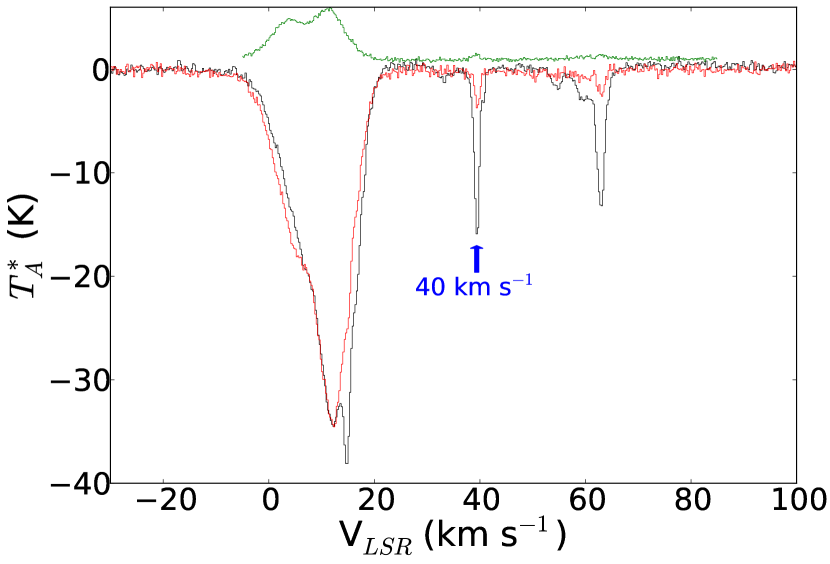
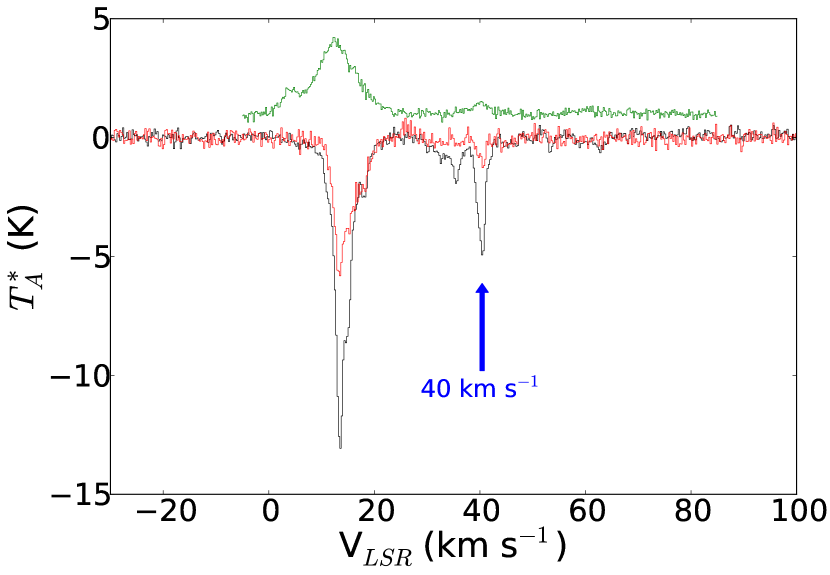
Figure 1: Spectra of the $\textrm{H}_{2}\textrm{CO}$ $1_{10}-1_{11}$ (black), $2_{11}-2_{12}$ (red), and ${}^{13}\textrm{CO}$ 1-0 (green) lines toward G43.17+0.01 (left) and G43.16-0.03 (right). The $\textrm{H}_{2}\textrm{CO}$ spectra are shown continuum-subtracted, and the ${}^{13}\textrm{CO}$ spectrum is offset by +1 K for clarity. The GBT $2_{11}-2_{12}$ spectra are multiplied by a factor of 9 so the smaller lines can be seen. The blue arrow marks the 40 km s^-1 cloud GRSMC 43.30-0.33 that we discuss in this paper.

We focus on the “foreground” line at $\sim 40$ km s^-1, since it is not associated with the extremely massive W49 region, which is dominated by gravity and stellar feedback rather than pure turbulence. The cloud is shown in Figure 2. Additional $\textrm{H}_{2}\textrm{CO}$ spectra of surrounding sources that are both bright at 8–1100 $\mu\textrm{m}$ and within the ${}^{13}\textrm{CO}$ contours of the cloud have $\textrm{H}_{2}\textrm{CO}$ $2_{11}-2_{12}$ detections at $\sim 10$ or $\sim 60$ km s^-1. The detections of dense gas at these other velocities, and corresponding nondetections of $2_{11}-2_{12}$ at 40 km s^-1, indicate that the star-forming clumps apparent in the infrared in Figure 2 are not associated with the 40 km s^-1 cloud.

The $\textrm{H}_{2}\textrm{CO}$ lines are observed in the outskirts of the cloud, not at the peak of the ${}^{13}\textrm{CO}$ emission. The cloud spans $\sim 0.6^{\circ}$, or $\sim 30$ pc at $D=2.8$ kpc (Roman-Duval et al., 2009). It is detected in $1_{10}-1_{11}$ absorption at all 6 locations observed in $\textrm{H}_{2}\textrm{CO}$ (Figure 2), but $2_{11}-2_{12}$ is only detected in front of the W49 HII region because of the higher signal-to-noise at that location. The detected ${}^{13}\textrm{CO}$ and $\textrm{H}_{2}\textrm{CO}$ lines are fairly narrow, with $\textrm{H}_{2}\textrm{CO}$ FWHM ranging from $\Delta v\sim 1.3-2.8$ km s^-1 and ${}^{13}\textrm{CO}$ widths from $\Delta v\sim 1.5-4.6$ km s^-1, where the largest line-widths are from averaging over the largest scales in the cloud. The ${}^{13}\textrm{CO}$ lines are 50–100% wider than the $\textrm{H}_{2}\textrm{CO}$ lines. This greater linewidth is due to high optical depth in the more common isotopologues, since $\textrm{C}^{18}\textrm{O}$ has the same linewidth as $\textrm{H}_{2}\textrm{CO}$ and ${}^{12}\textrm{CO}$ is $3\times$ wider (Plume et al., 2004, their Table 4).

The highest ${}^{13}\textrm{CO}$ contours are observed as a modest infrared dark cloud in Spitzer 8 $\mu\textrm{m}$ images, but no dust emission peaks are observed at 500 $\mu\textrm{m}$ (Herschel; Traficante et al., 2011) or 1.1 mm (Bolocam; Aguirre et al., 2011; Ginsburg et al., 2013) associated with the dark gas. This is an indication that the cloud is not dominated by gravity – no massive dense clumps are present within this cloud.

The cloud’s density is the key parameter we aim to measure, so we first determine the cloud-averaged properties based on ${}^{13}\textrm{CO}$ 1-0. The cloud has mass in the range $M_{CO}=1-3\times 10^{4}$ $M_{\odot}$ in a radius $r=15$ pc as measured from the integrated ${}^{13}\textrm{CO}$ map using an optical depth estimate and abundance from Roman-Duval et al. (2010), so its mean density is $\rho(\textrm{H}_{2})\approx 10-30$ $\textrm{cm}^{-3}$ assuming spherical symmetry (see Appendix A). If we instead assume a cubic volume, as is done in simulations, the mean density is lower by a factor $\pi/6$. Simon et al. (2001) report a mass $M_{CO}=6\times 10^{4}M_{\odot}$ and $r=13$ pc, yielding a density $\rho(\textrm{H}_{2})=100$ $\textrm{cm}^{-3}$, which is consistent with our estimates. Roman-Duval et al. (2010) break the cloud apart into 3 separate objects for their analysis, GRSMC 43.04-0.11, GRSMC 43.24-00.31, and GRSMC 43.14-0.36. All three have the same velocity to within 1 km s^-1, but they show slight discontinuities in position-velocity space. These discontinuities are morphologically consistent with gaps seen in turbulent simulations, validating our assessment of the cloud as a single object, but as a maximally conservative estimate we use the density of the northmost “clump” GRSMC 43.04-0.11, which overlaps our target line of sight, as an upper limit. It has density $\rho\approx 120~{}\textrm{cm}^{-3}$, but we use $\rho<200$ $\textrm{cm}^{-3}$ as a slightly more conservative limit to allow for modest uncertainties in optical depth, radius, and abundance.

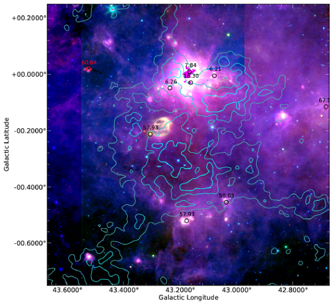
Figure 2: The GRSMC 43.30-0.33 cloud. The background image shows Herschel SPIRE 70 $\mu\textrm{m}$ (red), Spitzer MIPS 24 $\mu\textrm{m}$ (green), and Spitzer IRAC 8 $\mu\textrm{m}$ (blue) with the GRS ${}^{13}\textrm{CO}$ (Jackson et al., 2006) integrated image from $v_{LSR}=36$ km s^-1 to $v_{LSR}=43$ km s^-1 at contour levels of 1, 2, and 3 K km s^-1 superposed in cyan contours. The red and black circles show the locations and beam sizes of the $\textrm{H}_{2}\textrm{CO}$ observations, and their labels indicate the LSR velocity of the deepest absorption line in the spectrum. The W49 HII region is seen behind some of the faintest ${}^{13}\textrm{CO}$ emission. The dark swath in the 8 and 24 $\mu\textrm{m}$ emission going through the peak of the ${}^{13}\textrm{CO}$ emission in the lower half of the image is a low optical depth infrared dark cloud associated with this cloud. The two pointings examined in this paper and shown in Figures 1 and 3 are labeled by their peak LSR velocities, 7.84 and 16.30, for G43.17+0.01 and G43.16-0.03 respectively. They are separated by about 1 pc at the distance to the 40 km s^-1 cloud.

3 Modeling $\textrm{H}_{2}\textrm{CO}$

In order to infer densities using the $\textrm{H}_{2}\textrm{CO}$ densitometer, we use the low-temperature collision rates given by Troscompt et al. (2009) with RADEX using the large velocity gradient (LVG) approximation (van der Tak et al., 2007) to build a grid of predicted line properties covering 100 densities $\rho(\textrm{H}_{2})=10-10^{8}$ $\textrm{cm}^{-3}$, 10 temperatures $T=5-50$ K, 100 column densities $N(\textrm{o-H}_{2}\textrm{CO})=10^{11}-10^{16}$ $\textrm{cm}^{-2}$, and 10 $\textrm{H}_{2}$ ortho-to-para ratios $OPR=0.001-3.0$.

The $\textrm{H}_{2}\textrm{CO}$ densitometer measurements are shown in Figure 3. The figures show optical depth spectra, given by the equation

$$\tau=-\ln\left(\frac{S_{\nu}+2.73\mathrm{~{}K}}{\bar{C_{\nu}}+2.73\mathrm{~{}K}}\right)$$ (1)

where $S_{\nu}$ is the spectrum (with both the line and continuum included) and $\bar{C_{\nu}}$ is the measured continuum, both in Kelvin. The cosmic microwave background temperature is added to the continuum since $\textrm{H}_{2}\textrm{CO}$ can be seen in absorption against it, though toward W49 it is negligible.

Since the W49 lines of sight are clearly on the outskirts of the foreground cloud, not through its center, it is unlikely that these lines of sight correspond to a centrally condensed density peak (e.g., a core). The comparable line ratios observed through two different lines of sight separated by $\sim 1$ pc supports this claim, since if either line was centered on a core, we would observe a much higher $2_{11}-2_{12}$ optical depth.

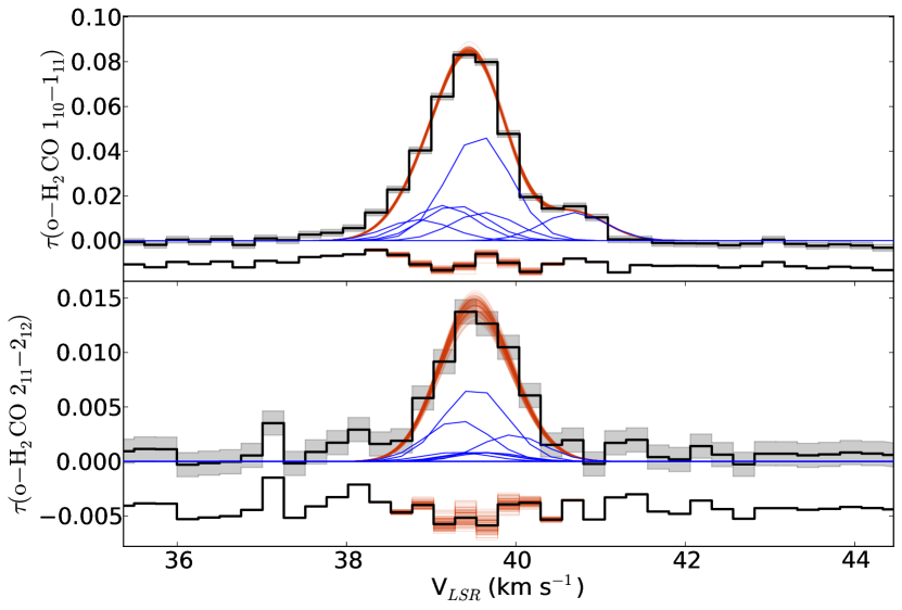
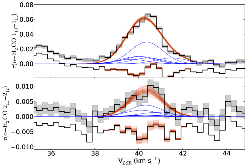
Figure 3: Optical depth spectra of the $1_{10}-1_{11}$ and $2_{11}-2_{12}$ lines toward the two W49 lines of sight, G43.17+0.01 (left) and G43.16-0.03 (right). The grey bars show the 1-$\sigma$ error bars on each data point. The red lines show 100 realizations from an MCMC fit of the $\textrm{o-H}_{2}\textrm{CO}$ $1_{10}-1_{11}$ and $2_{11}-2_{12}$ lines using the LVG model grid. The blue lines show the hyperfine components that make up the $1_{10}-1_{11}$ and $2_{11}-2_{12}$ lines for the optimal fit; the $1_{10}-1_{11}$ line is resolved into two components in the G43.17+0.01 spectrum. The residuals of the fit are shown offset below the spectra with the residuals of the above 100 MCMC realizations overplotted in red. The optical depth ratio falls in a regime where gas temperature has very little effect on the observed depth and there is no degeneracy between low and high densities (Ginsburg et al., 2011).

We performed fits of the optical depth spectra to each line independently using a Markov-Chain Monte Carlo (MCMC) approach (Ginsburg & Mirocha, 2011; Patil et al., 2010). In both lines of sight, we found that the centroids and widths agreed (see Table 1).

From this point on, we discuss only the G43.17+0.01 line of sight ($V_{LSR}=7.84$ km s^-1 in Figure 2), since it is well-fit by a single component and has high signal-to-noise. Since both lines of sight sample the same CO cloud, all of the measurements below are most strongly constrained by the G43.17+0.01 line of sight and the G43.16-0.03 line of sight provides no additional information.

Table 1: Fitted Parameters

	$1_{10}-1_{11}$	$2_{11}-2_{12}$
G43.17+0.01
Centroid	$39.54^{+0.01}_{-0.01}$	$39.55^{+0.06}_{-0.06}$
Width	$0.37^{+0.01}_{-0.02}$	$0.45^{+0.07}_{-0.08}$
Peak	$0.114^{+0.004}_{-0.004}$	$0.015^{+0.002}_{-0.002}$
Integral	$0.107^{+0.002}_{-0.002}$	$0.016^{+0.002}_{-0.002}$
Ratio	$6.49^{+0.84}_{-0.67}$
G43.16-0.03
Centroid	$40.35^{+0.04}_{-0.03}$	$40.36^{+0.23}_{-0.22}$
Width	$0.72^{+0.04}_{-0.04}$	$0.84^{+0.23}_{-0.31}$
Peak	$0.071^{+0.003}_{-0.003}$	$0.008^{+0.002}_{-0.002}$
Integral	$0.130^{+0.005}_{-0.005}$	$0.018^{+0.004}_{-0.004}$
Ratio	$7.32^{+2.31}_{-1.43}$

Centroid and width are in km s^-1, peak is unitless (optical depth), and the integral is in optical depth times km s^-1. The errors represent 95% credible intervals (2-$\sigma$).

4 Turbulence and the $\textrm{H}_{2}\textrm{CO}$ cm lines

Supersonic interstellar turbulence can be characterized by its driving mode, Mach number $\mathcal{M}$, and magnetic field strength. We start by assuming the gas density follows a lognormal distribution, defined as

$$P_{V}(s)=\frac{1}{\sqrt{2\pi\sigma_{s}^{2}}}\exp\left[-\frac{(s+\sigma_{s}^{2}/2)^{2}}{2\sigma_{s}^{2}}\right]$$ (2)

(Padoan & Nordlund, 2011; Molina et al., 2012) where the subscript $V$ indicates that this is a volume-weighted density distribution function. The parameter $s$ is the logarithmic density contrast, $s\equiv\ln(\rho/\rho_{0})$ for mean volume-averaged density $\rho_{0}\equiv\langle\rho\rangle_{V}$. The width of the turbulent density distribution is given by

$$\sigma_{s}^{2}=\ln\left(1+b^{2}\mathcal{M}^{2}\frac{\beta}{\beta+1}\right)$$ (3)

where $\beta=2c_{s}^{2}/v_{A}^{2}=2\mathcal{M}_{A}^{2}/\mathcal{M}^{2}$ and $b$ ranges from $b\sim 1/3$ (solenoidal, divergence-free forcing) to $b\sim 1$ (compressive, curl-free) forcing (Federrath et al., 2008, 2010). $c_{s}$ is the isothermal sound speed ($s$ here is short for ‘sound’), $v_{A}$ is the Alfvén speed, and $\mathcal{M}_{A}$ is the Alfvénic Mach number.

The observed $\textrm{H}_{2}\textrm{CO}$ line ratio roughly depends on the mass-weighted probability distribution function (as opposed to the volume-weighted distribution function, which is typically reported in simulations). For each $\textrm{H}_{2}\textrm{CO}$ molecule, the likelihood of absorbing a background photon is set by the level population in the lower energy state, which is controlled by the $\textrm{H}_{2}$ density as long as the line is optically thin (which is the case we treat here).

For a given ‘cell’ at density $\rho$, the optical depth is given by the number (or mass) of particles in that cell $M(\rho)=V\cdot\rho$ (assuming a fixed cell volume $V$) times the optical depth $\Upsilon_{\nu,p}$, where the subscript $p$ indicates that this is an optical depth per particle. The total optical depth is the optical depth per cell integrated over the probability distribution function, $\tau_{tot}=\int M(\rho)\Upsilon_{\nu,p}P_{V}(\rho)d\rho$, which is equivalent to $\tau_{tot}=\int\Upsilon_{\nu,p}P_{M}(\rho)d\rho$ using the definition of mass-weighted density $P_{M}(\rho)\equiv(\rho/\rho_{0})P_{V}(\rho)$.

Following this derivation, we use the RADEX models of the $\textrm{H}_{2}\textrm{CO}$ lines, which are computed assuming a fixed local density, as a starting point to model the observations of $\textrm{H}_{2}\textrm{CO}$ in turbulence. Starting with a fixed volume-averaged density $\rho_{0}$, we compute the observed $\textrm{H}_{2}\textrm{CO}$ optical depth $\tau_{\nu}$ in both the $1_{10}-1_{11}$ and $2_{11}-2_{12}$ line by averaging over the mass-weighted density distribution and redefining the equations with a logarithmic differential.

$$\tau_{\nu}(\rho_{0}) = \int_{-\infty}^{\infty}\Upsilon_{\nu,p}(\rho)P_{M}(\ln\rho/\rho_{0})d\ln(\rho/\rho_{0})$$ (4)

$$= \int_{-\infty}^{\infty}\Upsilon_{\nu,p}(\rho_{0}e^{s})P_{M}(s)ds$$ (5)

$\Upsilon_{\nu,p}(\rho)$ is the optical depth per particle at a given density, where $N_{p}$ is the column density (per km s^-1 pc^-1) from the LVG model. We assume a fixed abundance of $\textrm{o-H}_{2}\textrm{CO}$ relative to $\textrm{H}_{2}$ (i.e., the $\textrm{H}_{2}\textrm{CO}$ perfectly traces the $\textrm{H}_{2}$).

Figure 4 shows the result of this integral for an abundance of $\textrm{o-H}_{2}\textrm{CO}$ relative to $\textrm{H}_{2}$, $X(\textrm{o-H}_{2}\textrm{CO})=10^{-8.5}$, where the X-axis shows the volume-averaged number density $\rho_{0}\equiv\rho(\textrm{H}_{2})$ and the Y-axis shows the observable optical depth ratio of the two $\textrm{H}_{2}\textrm{CO}$ centimeter lines. The LVG model, which assumes a single density (or a Dirac $\delta$ function as the density distribution), is shown along with the PDF-weighted-average versions of the model that take into account realistic turbulent gas distributions.

The $\textrm{H}_{2}\textrm{CO}$ $2_{11}-2_{12}$ line requires a higher density to be “refrigerated” into absorption. As a result, any spread of the density distribution means that a higher fraction of the mass is capable of exciting the $2_{11}-2_{12}$ line. Wider distributions increase the $2_{11}-2_{12}$ line more than the $1_{10}-1_{11}$ line and decrease the ($1_{10}-1_{11}$)/($2_{11}-2_{12}$) ratio.

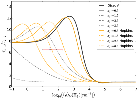
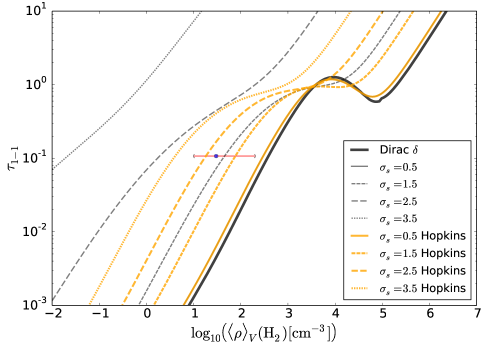
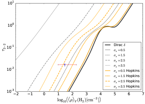
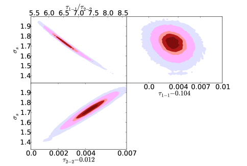
Figure 4: The predicted $\textrm{H}_{2}\textrm{CO}$ $1_{10}-1_{11}$/$2_{11}-2_{12}$ ratio and optical depths as a function of the ${}^{13}\textrm{CO}$-derived volume-weighted mean density for a fixed abundance relative to $\textrm{H}_{2}$ $X(\textrm{o-H}_{2}\textrm{CO})=10^{-8.5}$ with $\textrm{H}_{2}$ ortho/para ratio 1.0. The different lines show the effect of averaging over different mass distributions as identified in the legend. The thick solid line shows the predicted values with no averaging (i.e., a $\delta$-function density distribution); the other solid line shows $\sigma_{s}=0.5$ for both distributions (they overlap). The blue point shows the G43.17+0.01 measurement. The horizontal red error bars show the limits on the mean volume density, $\langle\rho\rangle_{V}$, and the vertical blue error bars show the 95% credible interval for the $\textrm{H}_{2}\textrm{CO}$ line measurements. The bottom-right figure shows the allowed $\sigma_{s}$ parameter space for the lognormal distribution given the $1_{10}-1_{11}$ and $2_{11}-2_{12}$ measurements and their ratio; the values are reported in Table 2. The contours indicate the 25% (dark red), 50% (red), 68% (light red), 95% (pink), and 99.7% (blue-grey) credible regions.

4.1 The $\rho$-PDF in GRSMC 43.30-0.33

We use the density measurements in GRSMC 43.30-0.33 to infer properties of that cloud’s density distribution. The observed line ratio for the G43.17+0.01 sightline in GRSMC 43.30-0.33 is shown in Figure 4 as a blue point. The position of this point on the x-axis is set by the ${}^{13}\textrm{CO}$-derived volume-averaged density, while its y-axis position in the three subplots reflects the $\textrm{H}_{2}\textrm{CO}$ measurements reported in Table 1.

Table 2: Fitted Distribution Parameters

Parameter	Lognormal	Hopkins
$X(\textrm{H}_{2}\textrm{CO})=10^{-8.5}$
$\sigma_{s}$	1.7${}^{0.2}_{0.2}$	-
$\sigma_{s}|\mathcal{M}$	1.7${}^{0.2}_{0.1}$	-
$b|\mathcal{M}$	$>0.56$	-
$X(\textrm{H}_{2}\textrm{CO})=10^{-9.0}$
$\sigma_{s}$	1.5${}^{0.1}_{0.1}$	2.7${}^{0.5}_{0.5}$
$T$	-	0.31${}^{0.08}_{0.10}$
$\sigma_{s}|\mathcal{M}$	1.5${}^{0.1}_{0.1}$	2.5${}^{0.5}_{0.5}$
$T|\mathcal{M}$	-	0.29${}^{0.08}_{0.08}$
$b|\mathcal{M}$	$>0.41$	$>0.71$

The error bars represent 95% credible intervals. For the $b$ parameter, only the lower limit is shown. The $|\mathcal{M}$ notation indicates that the parameter measurement includes the constraints imposed by the Mach number measurements, for which we have adopted $\mathcal{M}_{3D}=5.1\pm 1.5$, where $\sigma_{\mathcal{M}}=1.5$ is the standard deviation of the normal distribution we used to represent the Mach number. The $-$’s indicate disallowed parameter space (top) or parameters that are not part of the distribution (bottom).

Assuming the thermal dominates the magnetic pressure ($\beta>>1$), we can fit $\sigma_{s}$ from the model distributions in Figure 4. Using two different forms for the density distribution, and using only the $\tau$ measurements as a constraint, we derive the value of $\sigma_{s}$ in Table 2 and seen in the bottom-right panel of Figure 4.

Direct measurements of the Mach number from line-of-sight velocity dispersion measurements allow for further constraints on the distribution shape. Assuming a temperature $T=10$ K, consistent with both the $\textrm{H}_{2}\textrm{CO}$ and CO observations (Plume et al., 2004), the sound speed in molecular gas is $c_{s}=0.19$ km s^-1. The gas is unlikely to be much colder, so this sound speed provides an upper limit on the Mach number. The observed line FWHM in G43.17 is 0.95 km s^-1 for $\textrm{H}_{2}\textrm{CO}$ and 1.7 km s^-1 for ${}^{13}\textrm{CO}$ 1-0, so the 3-D Mach number of the turbulence is (Schneider et al., 2013)

$$\mathcal{M}_{3D}\equiv 3^{1/2}\mathcal{M}_{1D}\approx\frac{3^{1/3}}{(8\ln 2)^{1/2}}FWHM/c_{s}$$ (6)

or $\mathcal{M}_{3D}=3.8-6.6$ , ranging from the $\textrm{H}_{2}\textrm{CO}$ to the ${}^{13}\textrm{CO}$ width along the G43.17+0.01 line of sight. However, we note that the velocity dispersion for the whole cloud is larger.

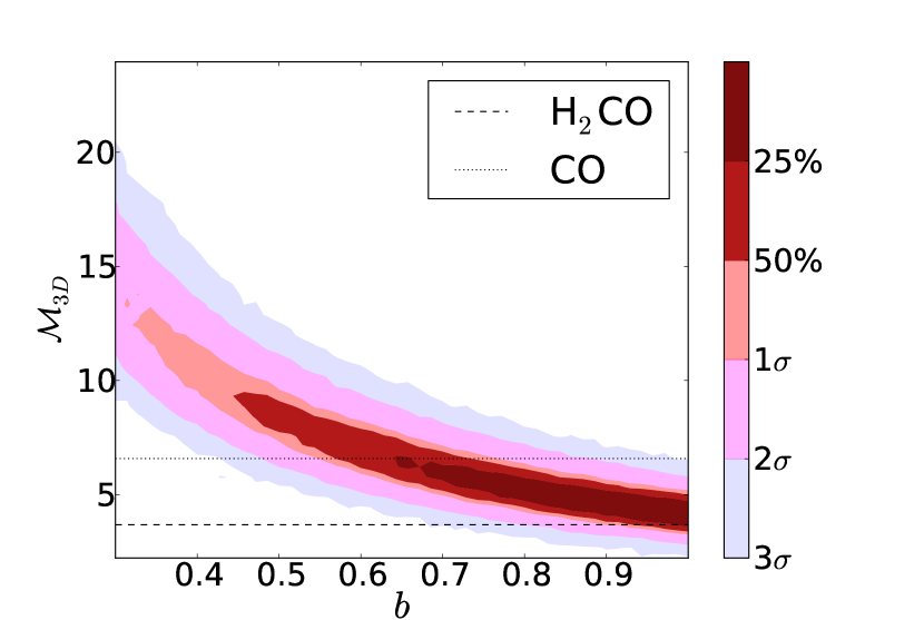
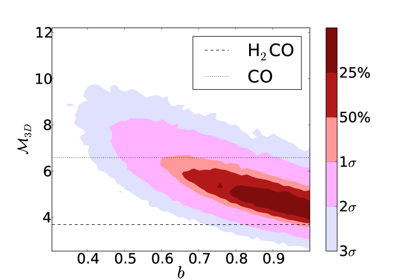
Figure 5: Contours of the MCMC fit to the $\textrm{H}_{2}\textrm{CO}$ optical depths with the cloud mean density restricted to $10~{}\textrm{cm}^{-3}<\langle\rho\rangle_{V}<200~{}\textrm{cm}^{-3}$. The contour levels indicate the regions in which 25, 50, 68, 95, and 99.7% of the MCMC samples are included. The left plot shows the parameter space allowed with no constraints on the Mach number, indicating the mild degeneracy between Mach and $b$. The right plot shows the parameters derived using the constraints on the Mach number based on the G43.17+0.01 line of sight, $\mathcal{M}_{3D}\approx 5.1\pm 1.5$, which is halfway between the value inferred from the $\textrm{H}_{2}\textrm{CO}$ and ${}^{13}\textrm{CO}$ line widths. The horizontal lines in both plots represent the Mach numbers inferred from the $\textrm{H}_{2}\textrm{CO}$ and CO line widths via Equation 6. Both plots are marginalized over the other free parameters ($\sigma_{s}$, $\rho_{V}$, and the observed optical depth).

Using the observed range of Mach numbers along the G43.17+0.01 line of sight, we can constrain $b$ with Equation 3. Figure 5 shows the Mach number-$b$ parameter space allowed by the observed volume density and $\textrm{H}_{2}\textrm{CO}$ lines both with and without the Mach number constraint imposed. If we assume the Mach number is approximately halfway between the $\textrm{H}_{2}\textrm{CO}$ and CO based measurements, with a dispersion that includes both, we can constrain $b>0.56$ (see Table 2).

4.1.1 The Hopkins distribution

As one possible alternative, we use the Hopkins (2013) density distribution,

$$P_{V}(\ln\rho)d\ln\rho=I_{1}(2\sqrt{\lambda u})e^{-(\lambda+u)}\lambda du$$ (7)

where $u\equiv\lambda/(1+T)-\ln(\rho/\rho_{0})/T$ and $\lambda\equiv\sigma^{2}_{\ln\rho/\rho_{0}}/(2T^{2})$ (Equation 5 in Hopkins, 2013, modified such that $\rho_{0}$ is not assumed to be unity). The distribution is governed by a width $\sigma_{s}\equiv\sigma_{\ln\rho/\rho_{0}}$ and an “intermittency” parameter $T$ that indicates the deviation of the distribution from lognormal. The intermittency parameter is described in Hopkins (2013) as a unitless parameter which increases with Mach number and is correlated with the strength of the deviations from the mean turbulent properties as a function of time. Its physical meaning beyond these simple correlations is as yet poorly understood.

We use $T$ values given the $T-\sigma_{s}$ and $T-\mathcal{M}_{C}$ relations fitted to measurements from a series of simulations (Kowal & Lazarian, 2007; Kritsuk et al., 2007; Schmidt et al., 2009; Federrath et al., 2010; Konstandin et al., 2012; Molina et al., 2012; Federrath, 2013), where $\mathcal{M}_{c}$ is the compressive Mach number, e.g. $\mathcal{M}_{c}=b\mathcal{M}$. The values are given by

$$T(\sigma_{s})=0.25\ln(1+0.25\sigma_{s}^{4}\left(1+T(\sigma_{s})\right)^{-6})$$ (8)

Equation 8 is a transcendental equation, so we use root-finding to determine $T$.

Assuming the same abundance as above, $X(\textrm{H}_{2}\textrm{CO})=10^{-8.5}$, the Hopkins distribution is incompatible with our observations for the $T-\sigma$ relations considered in Hopkins (2013) and the other $T$ values and relations explored in Figure 6b. Figure 6a shows how the Hopkins and lognormal distributions differ; the Hopkins distribution is more sharply peaked and includes less gas above its peak density. The incompatibility with our observations arises because the Hopkins distribution produces lower mass-weighted densities than the lognormal.

However, the Hopkins distribution is compatible with our observations if a lower abundance is assumed. Using the Hopkins distribution with $X(\textrm{H}_{2}\textrm{CO})=10^{-9}$, we find $\sigma_{s}\sim 2.5$ (see Table 2). This value is compatible with the observed Mach numbers. Using the relation

$$b\mathcal{M}=\mathcal{M}_{c}\approx 20T$$ (9)

from Hopkins (2013) Figure 3, we can derive a lower limit $b>0.7$. However, there is additional intrinsic uncertainty in the coefficient in Equation 9 that comes from fitting the relation to simulated data, and we have not accounted for this uncertainty.

The Hopkins distribution is compatible with our observations, but requires relatively extreme values of the standard deviation and $b$ parameters. We explored a few alternate realizations of the Hopkins distribution’s $T-\sigma$ relation, with results shown in Figure 6. Independent of the form of the Hopkins distribution chosen, it is more restrictive than the lognormal distribution.

4.2 Discussion

The restrictions on $\sigma_{s}$ and $b$ using either the lognormal or Hopkins density distribution are indications that compressive forcing must be a significant, if not dominant, mode in this molecular cloud. However, there are no obvious signs of cloud-cloud collision or interaction with a supernova that might directly indicate what is driving the turbulence.

Most of the systematic uncertainties tend to require a greater $b$ value, while we have already inferred a lower limit that is moderately higher than others have observed (Brunt, 2010; Kainulainen et al., 2013). Temperatures in GMCs are typically 10-20 K, and we assumed 10 K: warmer temperatures increase the sound speed and therefore decrease the Mach number. If the cloud is warmer, the $b$ values again must be higher to account for the measured $\sigma_{s}$. Magnetic fields similarly have the inverse effect of $b$ on $\sigma_{s}$, with decreasing $\beta$ requiring higher $b$ for the same $\sigma_{s}$.

The only systematic that operates in the opposite direction is the abundance of $\textrm{o-H}_{2}\textrm{CO}$. Lower abundance shifts all curves in Figure 4 up and to the right, which decreases $\sigma_{s}$ and therefore allows for a lower $b$ for fixed Mach number. However, abundances lower than $X=10^{-9}$ are rarely observed except in Galactic cirrus clouds (Turner et al., 1989) and highly shocked regions like the cirumnuclear disk around Sgr A* (Pauls et al., 1996), so the measurements in Table 2 should bracket the allowed values. While we only explored two possible abundances in detail, note that the $\sigma_{s}$ values derived from the lognormal distribution vary little over half-dex changes in abundance (Table 2), indicating that this measurement at least is robust to abundance assumptions.

We explore these caveats and others in more detail in the Appendix.

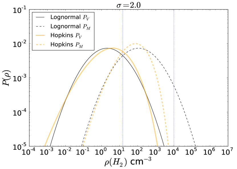
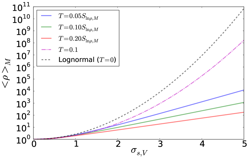
Figure 6: Left: Example volume- and mass-weighted density distributions with $\sigma_{s}=2.0$. The vertical dashed lines show $\rho=15$ $\textrm{cm}^{-3}$ and $\rho=10^{4}$ $\textrm{cm}^{-3}$, approximately corresponding to the volume-weighted mean density $\langle\rho\rangle_{V}$ of GRSMC 43.30-0.33 from ${}^{13}\textrm{CO}$ and the $\textrm{H}_{2}\textrm{CO}$-derived density, respectively. Note that the peaks of the distributions do not correspond to their means, since the mean of the lognormal distribution depends on its variance. Right: The relationship between the mass-weighted mean density $\langle\rho\rangle_{M}$ and the width of the volume-weighted density PDF $P_{V}(\rho)$ for the lognormal distribution and different realizations of the Hopkins (2013) distribution with $\rho_{0}=1$. We show different forms of the $T-\sigma$ relation using $T=c\cdot S_{\ln\rho,M}$, which is an approximation of Equation 8, and one example of $T=$ constant. It is clear that, for a given distribution width, the Hopkins distribution always puts less mass at the highest densities than the lognormal distribution.

5 Conclusions

We demonstrate the use of a novel method of inferring parameters of the density probability distribution function in a molecular cloud using $\textrm{H}_{2}\textrm{CO}$ densitometry in conjunction with ${}^{13}\textrm{CO}$-based estimates of total cloud mass. We have measured the standard deviation of the lognormal turbulence density distribution $1.5<\sigma_{s}<1.9$ and placed a lower limit on the compressiveness parameter $b>0.4$. Both measurements are robust to the assumed cloud density, $\textrm{H}_{2}\textrm{CO}$ abundance, and other assumptions.

Our data show evidence for compressively driven turbulence in a non-star-forming giant molecular cloud. Since this cloud represents a typical molecular cloud, it is likely that compressive driving is a common feature of all molecular clouds.

This new method opens the possibility of investigating the drivers of turbulence more directly, e.g. by measuring the shape of the density PDF both within spiral arms and in the inter-arm regions. The main requirements for applying this technique are a moderately accurate measurement of the mean cloud density, which can easily be provided by ${}^{13}\textrm{CO}$ surveys such as the GRS, and a high signal-to-noise measurement of the 2 cm and 6 cm $\textrm{H}_{2}\textrm{CO}$ lines.

A precise measurement of the Mach number of the cloud will allow measurements of $b$ rather than the limits we have presented here. Investigations of the predicted observed velocity dispersion and line strengths in both $\textrm{H}_{2}\textrm{CO}$ and ${}^{13}\textrm{CO}$ in simulations of turbulent clouds should provide the details needed to take this next step.

Finally, the general approach of accounting for a density distribution by averaging over the contribution to the line profile at each density should be generally applicable to any molecular line observations as long as the lines are optically thin.

6 Acknowledgements

We thank Erik Rosolowsky and Ben Zeiger for useful discussions and comments that greatly improved the clarity of the paper. We thank the anonymous referee for a timely and constructive report that helped improve the paper. This publication makes use of molecular line data from the Boston University-FCRAO Galactic Ring Survey (GRS). The GRS is a joint project of Boston University and Five College Radio Astronomy Observatory, funded by the National Science Foundation under grants AST-9800334, AST-0098562, & AST-0100793. This research made use of Astropy, a community-developed core Python package for Astronomy (http://astropy.org; The Astropy Collaboration et al., 2013). It also made use of pyspeckit, an open source python-based package for spectroscopic data analysis (%****␣ms.tex␣Line␣1100␣****http://pyspeckit.readthedocs.org; Ginsburg & Mirocha, 2011). The dendrogramming was performed using the python dendrogram package described at http://dendrograms.org. JD acknowledges the support of the NSF through the grant AST-0707713. CF is supported from the Australian Research Council with a Discovery Projects Fellowship (Grant DP110102191).

Facilities: GBT, Arecibo, FCRAO, CSO

Appendix A Assumptions, caveats, and uncertainties

We explore the various caveats and assumptions that have been treated above in more detail here.

The precise density measurements presented here are based on large velocity gradient approximations (Sobolev, 1957) for the escape probability of line radiation from the cloud. This method is widely used but remains an approximation. In the case of $\textrm{H}_{2}\textrm{CO}$, it has been tested with a variety of codes (van der Tak et al., 2007; Henkel et al., 1983) but is subject to uncertainties in the velocity gradient and system geometry. However, in the case of the observations in this paper, the lines were observed in the optically thin regime, and the LVG approximation should not affect our results.

The collision rates of $\textrm{H}_{2}\textrm{CO}$ with p-$\textrm{H}_{2}$, o-$\textrm{H}_{2}$, and He are estimated based on computer simulations of the particles. Troscompt et al. (2009) improved upon the measurements of Green (1991), bringing the typical collision rate uncertainty down from $\sim 50\%$ in the He-based approximation to $\sim 10\%$ using full models of ortho and para $\textrm{H}_{2}$. Wiesenfeld & Faure (2013) noted that the differences they observed from the Troscompt et al. (2009) results were $<10\%$, indicating that the methods they use are at least convergent & self-consistent to within $\sim 30\%$. Zeiger & Darling (2010) reported the results of using modified collision rates assuming a 50% error and noted that the resulting errors in the $\textrm{H}_{2}$ density were, in the worst case, $<0.3$ dex. With the improved Troscompt et al. (2009) collision rates, the model uncertainties are no longer dominated by collision rate uncertainties.

Abundance remains a serious concern, as most studies of $\textrm{o-H}_{2}\textrm{CO}$ abundance do not observe multiple transitions and therefore do not constrain the relative level populations. There are also general difficulties in measuring absolute abundance of molecules, as the absolute column of $\textrm{H}_{2}$ is rarely known with high accuracy. Most abundance measurements are above $X_{\textrm{o-H}_{2}\textrm{CO}}>10^{-9}$ (Dickens & Irvine, 1999; Liszt et al., 2006), except near Sgr A* (Pauls et al., 1996) and in Galactic cirrus clouds (Turner et al., 1989; Turner, 1993) where it is generally observed to have $10^{-10}<X_{\textrm{o-H}_{2}\textrm{CO}}<10^{-9}$. These measurements dictated the abundance boundaries we used in our analysis.

The ortho-to-para ratio of $\textrm{H}_{2}$ is a significant uncertainty in the models, since para-$\textrm{H}_{2}$ is more effective at “refrigerating” the $\textrm{H}_{2}\textrm{CO}$ molecules. Values of the ortho-to-para ratio $>1$ favor lower densities by $\sim 0.3$ dex, but we have used these lower densities in our analysis, and therefore our results are conservative. However, if the ortho-to-para ratio is in reality close to zero, the density PDF must be wider and $b$ correspondingly higher.

The “covering factor” of foreground clouds in front of background illumination sources is, in general, a major concern when performing absorption measurements. For the clouds presented in this work, the absorbing region is much larger than the background, as evidenced by the two lines-of-sight with similar optical depth ratios. However, for more detailed studies of density variations, EVLA observations can and should be employed.

The single largest uncertainty is related to the mean properties of the GMC. While we have accounted for these uncertainties by adopting a very conservative range of values for the mean density (covering two orders of magnitude), it is not entirely clear how the mean density of the cloud should be computed for comparison to simulations and the analytic distributions. Since this is a foreground cloud lying in front of a rich portion of the galactic plane, the best mass estimates will always come from molecular line observations, and therefore they are unlikely to be improved unless new wide-field CO observations are taken, e.g. with CCAT.

To validate our cloud mean density measurements, we have performed a dendrogram analysis (Rosolowsky et al., 2008) on the integrated ${}^{13}\textrm{CO}$ map of the GRSMC 43.30-0.33 cloud. We perform the analysis both on the large-scale $r\sim 20$ pc cloud, tracking down to 10 pc scales, and then on the individual clump that is directly in front of W49. We show the cloud density, computed using the assumptions stated in the text to convert ${}^{13}\textrm{CO}$ luminosity to mass, for three different geometrical assumptions described in the caption of Figure 7. While the clump densities are potentially higher than we assumed in the analysis, they are probably not the appropriate numbers to compare to the simulations we have cited, which are generally simulating entire molecular clouds and measuring the density distribution within a large box.

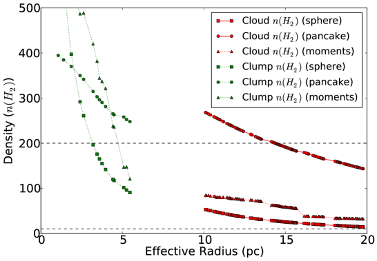
Figure 7: Results of a dendrogram analysis of the GRSMC 43.30-0.33 cloud and the northernmost ${}^{13}\textrm{CO}$ “clump” within that cloud. The data points represent successively higher (and therefore smaller) contours within the integrated ${}^{13}\textrm{CO}$ map. The shapes represent three different methods for extracting the volume: squares assume spherical symmetry using the effective radius of the contour, which is proportional to the square root of the number of pixels. Circles do the same, but assume that the line-of-sight radius is 2 pc (i.e., smaller than the observed plane-of-the-sky dimensions). The triangles show the volume of an ellipsoid using the moments of the contoured pixels, with volume $V=4/3\pi R_{maj}R_{min}^{2}$. The black dashed lines indicate the range of densities allowed in our fits.

References

- Aguirre et al. (2011) Aguirre, J. E. et al. 2011, ApJS, 192, 4
- Brunt (2010) Brunt, C. M. 2010, A&A, 513, A67
- Chabrier & Hennebelle (2010) Chabrier, G. & Hennebelle, P. 2010, ApJ, 725, L79
- Cho & Kim (2011) Cho, W. & Kim, J. 2011, MNRAS, 410, L8
- Collins et al. (2012) Collins, D. C., Kritsuk, A. G., Padoan, P., Li, H., Xu, H., Ustyugov, S. D., & Norman, M. L. 2012, ApJ, 750, 13
- Darling & Zeiger (2012) Darling, J. & Zeiger, B. 2012, ApJ, 749, L33
- Dickens & Irvine (1999) Dickens, J. E. & Irvine, W. M. 1999, ApJ, 518, 733
- Elmegreen (2011) Elmegreen, B. G. 2011, ApJ, 731, 61
- Federrath (2013) Federrath, C. 2013, MNRAS, In Press
- Federrath et al. (2011) Federrath, C., Chabrier, G., Schober, J., Banerjee, R., Klessen, R. S., & Schleicher, D. R. G. 2011, Physical Review Letters, 107, 114504
- Federrath & Klessen (2012) Federrath, C. & Klessen, R. S. 2012, ApJ, 761, 156
- Federrath & Klessen (2013) —. 2013, ApJ, 763, 51
- Federrath et al. (2008) Federrath, C., Klessen, R. S., & Schmidt, W. 2008, ApJ, 688, L79
- Federrath et al. (2009) —. 2009, ApJ, 692, 364
- Federrath et al. (2010) Federrath, C., Roman-Duval, J., Klessen, R. S., Schmidt, W., & Mac Low, M.-M. 2010, A&A, 512, A81
- Ginsburg et al. (2011) Ginsburg, A., Darling, J., Battersby, C., Zeiger, B., & Bally, J. 2011, ApJ, 736, 149
- Ginsburg et al. (2013) Ginsburg, A. et al. 2013, ArXiv e-prints
- Ginsburg & Mirocha (2011) Ginsburg, A. & Mirocha, J. 2011, Astrophysics Source Code Library, 9001
- Glover et al. (2010) Glover, S. C. O., Federrath, C., Mac Low, M.-M., & Klessen, R. S. 2010, MNRAS, 404, 2
- Green (1991) Green, S. 1991, ApJS, 76, 979
- Henkel et al. (1983) Henkel, C., Wilson, T. L., Walmsley, C. M., & Pauls, T. 1983, A&A, 127, 388
- Hennebelle & Chabrier (2008) Hennebelle, P. & Chabrier, G. 2008, ApJ, 684, 395
- Hennebelle & Chabrier (2009) —. 2009, ApJ, 702, 1428
- Hennebelle & Chabrier (2011) —. 2011, ApJ, 743, L29
- Hennebelle & Chabrier (2013) —. 2013
- Hopkins (2012) Hopkins, P. F. 2012, MNRAS, 423, 2037
- Hopkins (2013) Hopkins, P. F. 2013, Monthly Notices of the Royal Astronomical Society, 430, 1653
- Jackson et al. (2006) Jackson, J. M. et al. 2006, ApJS, 163, 145
- Kainulainen et al. (2013) Kainulainen, J., Federrath, C., & Henning, T. 2013
- Kainulainen & Tan (2012) Kainulainen, J. & Tan, J. C. 2012, ArXiv e-prints
- Klessen et al. (2000) Klessen, R. S., Heitsch, F., & Mac Low, M.-M. 2000, ApJ, 535, 887
- Konstandin et al. (2012) Konstandin, L., Girichidis, P., Federrath, C., & Klessen, R. S. 2012, ApJ, 761, 149
- Kowal & Lazarian (2007) Kowal, G. & Lazarian, A. 2007, ApJ, 666, L69
- Kritsuk et al. (2007) Kritsuk, A. G., Norman, M. L., Padoan, P., & Wagner, R. 2007, ApJ, 665, 416
- Kritsuk et al. (2011) Kritsuk, A. G., Norman, M. L., & Wagner, R. 2011, ApJ, 727, L20
- Krumholz et al. (2012) Krumholz, M. R., Dekel, A., & McKee, C. F. 2012, ApJ, 745, 69
- Krumholz & McKee (2005) Krumholz, M. R. & McKee, C. F. 2005, ApJ, 630, 250
- Liszt et al. (2006) Liszt, H. S., Lucas, R., & Pety, J. 2006, A&A, 448, 253
- Mangum & Wootten (1993) Mangum, J. G. & Wootten, A. 1993, ApJS, 89, 123
- Mangum et al. (1993) Mangum, J. G., Wootten, A., & Plambeck, R. L. 1993, ApJ, 409, 282
- Molina et al. (2012) Molina, F. Z., Glover, S. C. O., Federrath, C., & Klessen, R. S. 2012, MNRAS, 423, 2680
- Padoan et al. (2012) Padoan, P., Haugbølle, T., & Nordlund, Å. 2012, ApJ, 759, L27
- Padoan & Nordlund (2002) Padoan, P. & Nordlund, Å. 2002, ApJ, 576, 870
- Padoan & Nordlund (2011) —. 2011, ApJ, 730, 40
- Padoan et al. (2007) Padoan, P., Nordlund, Å., Kritsuk, A. G., Norman, M. L., & Li, P. S. 2007, ApJ, 661, 972
- Patil et al. (2010) Patil, A., Huard, D., & Fonnesbeck, C. J. 2010, Journal of Statistical Software, 35, 1
- Pauls et al. (1996) Pauls, T., Johnston, K. J., & Wilson, T. L. 1996, ApJ, 461, 223
- Plume et al. (2004) Plume, R. et al. 2004, ApJ, 605, 247
- Price et al. (2011) Price, D. J., Federrath, C., & Brunt, C. M. 2011, ApJ, 727, L21
- Roman-Duval et al. (2009) Roman-Duval, J., Jackson, J. M., Heyer, M., Johnson, A., Rathborne, J., Shah, R., & Simon, R. 2009, ApJ, 699, 1153
- Roman-Duval et al. (2010) Roman-Duval, J., Jackson, J. M., Heyer, M., Rathborne, J., & Simon, R. 2010, ApJ, 723, 492
- Rosolowsky et al. (2008) Rosolowsky, E. W., Pineda, J. E., Kauffmann, J., & Goodman, A. A. 2008, ApJ, 679, 1338
- Schmidt et al. (2009) Schmidt, W., Federrath, C., Hupp, M., Kern, S., & Niemeyer, J. C. 2009, A&A, 494, 127
- Schneider et al. (2013) Schneider, N. et al. 2013, ApJ, 766, L17
- Shetty et al. (2011a) Shetty, R., Glover, S. C., Dullemond, C. P., & Klessen, R. S. 2011a, MNRAS, 412, 1686
- Shetty et al. (2011b) Shetty, R., Glover, S. C., Dullemond, C. P., Ostriker, E. C., Harris, A. I., & Klessen, R. S. 2011b, MNRAS, 415, 3253
- Simon et al. (2001) Simon, R., Jackson, J. M., Clemens, D. P., Bania, T. M., & Heyer, M. H. 2001, ApJ, 551, 747
- Sobolev (1957) Sobolev, V. V. 1957, Soviet Ast., 1, 678
- Tang et al. (2013) Tang, X. D., Esimbek, J., Zhou, J. J., Wu, G., Ji, W. G., & Okoh, D. 2013, A&A, 551, A28
- The Astropy Collaboration et al. (2013) The Astropy Collaboration et al. 2013, ArXiv e-prints
- Traficante et al. (2011) Traficante, A. et al. 2011, MNRAS, 416, 2932
- Troscompt et al. (2009) Troscompt, N., Faure, A., Wiesenfeld, L., Ceccarelli, C., & Valiron, P. 2009, A&A, 493, 687
- Turner (1993) Turner, B. E. 1993, ApJ, 410, 140
- Turner et al. (1989) Turner, B. E., Richard, L. J., & Xu, L.-P. 1989, ApJ, 344, 292
- van der Tak et al. (2007) van der Tak, F. F. S., Black, J. H., Schöier, F. L., Jansen, D. J., & van Dishoeck, E. F. 2007, A&A, 468, 627
- Wiesenfeld & Faure (2013) Wiesenfeld, L. & Faure, A. 2013, MNRAS, 432, 2573
- Zeiger & Darling (2010) Zeiger, B. & Darling, J. 2010, ApJ, 709, 386