The ${\bf P}$-Laplace equation in domains
with multiple crack section via pencil operators

Abstract.

The $p$-Laplace equation

$$\nabla\cdot(|\nabla u|^{p-2}\nabla u)=0,\quad\mbox{where}\quad p>2,$$

in a bounded domain $\Omega\subset\mathbb{R}^{2}$, with inhomogeneous Dirichlet conditions on the smooth boundary $\partial\Omega$ is considered. In addition, there is a finite collection of curves

$$\Gamma=\Gamma_{1}\cup...\cup\Gamma_{m}\subset\Omega,\quad\mbox{on which we assume homogeneous Dirichlet conditions}\quad u=0,$$

modeling a multiple crack formation, focusing at the origin $0\in\Omega$. This makes the above quasilinear elliptic problem overdetermined. Possible types of the behaviour of solution $u(x,y)$ at the tip $0$ of such admissible multiple cracks, being a “singularity” point, are described, on the basis of blow-up scaling techniques and a “nonlinear eigenvalue problem”. Typical types of admissible cracks are shown to be governed by nodal sets of a countable family of nonlinear eigenfunctions, which are obtained via branching from harmonic polynomials that occur for $p=2$. Using a combination of analytic and numerical methods, saddle-node bifurcations in $p$ are shown to occur for those nonlinear eigenvalues/eigenfunctions.

1. Introduction

1.1. Models and preliminaries

We study solutions of the $p$-Laplace equation with Dirichlet boundary conditions in a bounded smooth domain $\Omega\subset\mathbb{R}^{2}$

(1.1) $$\left\{\begin{array}[]{cc}\nabla\cdot(|\nabla u|^{n}\nabla u)=0&\hbox{in}\quad\Omega,\\ u=f(x,y)&\hbox{on}\quad\Gamma,\\ u=g(x,y)&\hbox{on}\quad\partial\Omega,\\ \end{array}\right.$$

where $n>0$ is a fixed exponent ($n=p-2$, for the standard $p$-Laplacian but we use the parameter $n$ for convenience in our subsequent branching analysis) and $f(x,y)$ and $g(x,y)$ are given smooth functions. In our particular case, $\Omega$ is assumed to have a multiple crack $\Gamma$, as a finite collection of $m\geq 1$ curves

(1.2) $$\Gamma=\Gamma_{1}\cup\Gamma_{2}\cup...\cup\Gamma_{m}\subset\Omega\quad\mbox{such that each $\Gamma_{j}$ passes through the origin $0\in\Omega$ only}.$$

The origin is then the tip of this crack.

Moreover, we assume that, near the origin, in the lower half-plane $\{y<0\}$, all cracks asymptotically take a straight line form, i.e., as shown in Figure 1,

(1.3) $$\Gamma_{k}:\,\,x=\alpha_{k}(-y)(1+o(1)),\,\,y\to 0,\,\,\,k=1,2,...,m,\,\,\mbox{where}\,\,\,\alpha_{1}<\alpha_{2}<...<\alpha_{m}$$

are given constants. Thus, the precise statement of the problem assumes that (1.3) describes all the admissible cracks near the origin, i.e., no other straight-line cracks are considered. Indeed, through our analysis it will be determined that these are the only type of admissible cracks.

In our basic model, without loss of any generality (and to simplify the analysis), we assume a homogeneous Dirichlet condition at the crack:

(1.4) $$u=0\quad\mbox{on}\quad\Gamma,$$

that makes the problem overdetermined. So that, not any type of such multiple cracks (1.2), (1.3) are admissible.

For this problem, we ascertain important qualitative information about the behaviour of the solutions of problem (1.1). Especially important is the analysis close to the tip of the crack $\Gamma$, at least when the parameter $n$ is very close to zero (or $p$ very close to 2).

In particular the behaviour of the solutions at the singularity boundary points are described by some blow-up scaling techniques but also by a nonlinear eigenvalue problem through a branching argument. In other words we use an appropriate change of variable to transform the equations involved into the so-called pencil operators which reduces the problem to solve a 1$D$ spectral problem, allowing us to ascertain such an asymptotical behaviour at the tip of the crack.

Thus, using Pencil Operator Theory we first analyse the problem when $n=0$ reducing (1.1) to the well known Laplace equation. Most of the results presented for this problem are already known; such us the expression of its harmonic polynomials and their properties. However, we find convenient to show these properties within the pencil operator framework from which this work has been developed. Something that we believe is not widely known.

Furthermore, this analysis will be very important in the subsequent regarding the results of the $p$-Laplace problem (1.1). This problem is nonlinear and we cannot apply directly the ideas used for the linear case when $n=0$. Therefore, in order to arrive at the results we perform a branching analysis from the solutions of the problem when $n=0$ for which we have plenty of information.

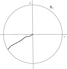
Figure 1. A formal one-crack model, $m=1$.

1.2. Laplace equation and pencil operators

Thus, first for $n=0$ we describe the behaviour of the solutions for the Laplace problem

(1.5) $$\Delta u=0\quad\mbox{in}\quad\,\,\Omega\;(=B_{1}),\quad u=f\,\,(\not\equiv 0)\quad\mbox{on}\quad\partial\Omega,\quad\mbox{with (\ref{Dir1})}.$$

at the tip of the crack (normally the origin), being a singularity boundary point.

To do so, blow-up scaling techniques and spectral theory of pencils of non self-adjoint operators are used. In particular, we perform a rescaling/change of variable of the form

(1.6) $$\textstyle{z=x/(-y)\quad\hbox{and}\quad\tau=-\ln(-y)\quad\mbox{for}\quad y<0.}$$

This rescaling corresponds to a blow-up scaling near the origin. In fact, this blow-up analysis assumes a kind of elliptic “evolution” approach for elliptic problems. We actually move the singularity point at the origin into an asymptotic convergence when $\tau\to\infty$.

Applying this rescaling (and then the separation variables method) we transform the Laplace equation into a pencil of non-self-adjoint operator, in particular for this case, a quadratic pencil operator of the form

$$(1+z^{2})(\psi^{*})^{\prime\prime}+2(\lambda+1)z(\psi^{*})^{\prime}+\lambda(\lambda+1)\psi^{*}=0,$$

for which we obtain two families of eigenfunctions

(1.7) $$\{\psi_{k_{+}}^{*}(z)\equiv\psi_{k,1}^{*}(z)\}\quad\hbox{and}\quad\{\psi_{k_{-}}^{*}(z)\equiv\psi_{k-1,2}^{*}(z)\}\quad\hbox{(defined in Section\;\ref{SLap})},$$

associated with two families of eigenvalues

(1.8) $$\lambda_{k}^{+}=-l,\quad l=1,2,3,...\quad\mbox{and}\quad\lambda_{k}^{-}=-l-1,\quad l=0,1,2,3,...\,,$$

Consequently, the application of the theory of pencil operators allows us to analyse the linear equation (1.5), with the geometrical structure assumed in this work.

Pencil operators are polynomials of the form

$$A(\lambda):=A_{0}+\lambda A_{1}+\cdots+\lambda^{n}A_{n},$$

where $\lambda\in{\mathbb{C}}$ is a spectral parameter and the coefficients $A_{i}$, with $i=0,1,\cdots,n$, are linear operators acting on a Hilbert space. Pencil operator theory appeared and was crucially used in the regularity and asymptotic analysis of elliptic problems in a seminal paper by Kondrat’ev [15] and also for parabolic problems in [14], where spectral problems, that are nonlinear (polynomial) in the spectral parameter $\lambda$, occurred. Later on, Mark Krein and Heinz Langer [16] made a fundamental contribution to this theory analyzing the spectral theory for strongly damped quadratic operator pencils.

Thus, using this well-developed spectral theory of non-self-adjoint operators, we are able to ascertain information about the solutions at the tip of the crack $\Gamma$ for the Laplace problem (1.5). Then, we deal with eigenfunctions (1.7) of a quadratic pencil of operator and not with a standard Sturm–Liouville problem (we keep this “blow-up scaling logic” for the analysis of the $p$-Laplace equation as well).

Consequently, and in particular for this simpler problem, we obtain that all the solutions with cracks at 0 must have the expression

(1.9) $$\textstyle{u(x,y)=w(z,\tau)=\sum_{(k\geq l)}{\mathrm{e}}^{-k\tau}[c_{k}\psi_{k,1}^{*}(z)+d_{k}\psi_{k-1,2}^{*}(z)],\quad\mbox{with}\quad c_{l}^{2}+d_{l}^{2}\neq 0,}$$

where $\psi_{k,1}^{*}(z)$ and $\psi_{k-1,2}^{*}(z)$ are two families of harmonic polynomials re-written in terms of a rescaled variable $z$ after performing the scaling (1.6).

Therefore, the main result established for the Laplace problem shows that in the first leading terms while approaching the origin, a linear combination of two families of eigenfunctions as classic harmonic polynomials. Then,

• If all $\{\alpha_{k}\}$ in (1.3) do not coincide with all $m$ subsequent zeros of any nontrivial linear combination

  (1.10) $$c_{l}\psi_{l,1}^{*}(z)+d_{l}\psi^{*}_{l-1,2}(z),\quad\mbox{with}\quad c_{l}^{2}+d_{l}^{2}\neq 0,$$

  then the multiple crack problem (1.5) cannot have a solution for any boundary Dirichlet data $f$ on $\partial\Omega$.

• However, if that is not the case, i.e. there is some $l$ for which the $m$ zeros of (1.10) coincide with $\{\alpha_{k}\}$, then there exists a solution $u$ and

  $$|u(x,y)|=O\left(|x,y|^{l}\right)\quad\hbox{as}\quad(x,y)\to(0,0).$$

Moreover and obviously, restricting to $\Gamma$ all types of admissible crack-containing expansions (1.9) (with closure in any appropriate functional space) fully describe all types of boundary data, which lead to the desired crack formation at the origin.

Thus, typical types of admissible cracks are shown to be governed by nodal sets of a countable family of harmonic polynomials, which are represented by pencil eigenfunctions, instead of their classical representation via a standard Sturm-Liouville problem; see Section 2. The analysis carried out for the case $n=0$ (the Laplace equation) will show that actually those types of cracks (1.3) are the only admissible ones.

1.3. Our main problem and main new results: $p$-Laplace equation

For the quasilinear problem (1.1), the obtained results for the Laplace crack problem (1.5) seem to be crucial. However, we need to change the strategy and base our analysis on a branching argument at $n=0$.

The main reason is due to the fact that for the previous Laplace equation we are able to obtain explicitly two families of negative eigenvalues associated, respectively, to two families of eigenfunctions. Indeed, from the expressions of the two families of eigenvalues (1.8) (see Section 2 below) and using the pencil operator theory [20], we can ascertain the coefficients of every eigenfunction explicitly as well.

However, following the same argument for the nonlinear PDE (1.1) it is not possible, in general, to get the corresponding families of eigenvalues and, hence, the associated eigenfunctions.

Therefore, using the knowledge we possess about the eigenfunctions of the quadratic pencil operator coming from the Laplace equation (1.5), and after performing the blow-up scaling (1.6), we carry out a branching analysis at $n=0$ obtaining information about the solutions/nonlinear eigenfunctions, at least, when $n$ is sufficiently close to zero and with the geometrical framework under consideration in this work.

Namely, we show that admissible crack configurations also correspond to nodal sets of nonlinear eigenfunctions, which we construct by branching at $n=0$ (or $p=2$) from the (re-written in terms of $z$) harmonic polynomials.

In particular, after performing the rescaling (1.6) we transform the $p$-Laplace problem (1.1) into a pencil operator (see the details in Section 3) which is indeed a nonlinear eigenvalue problem. Then, we construct a set of uniquely determined nonlinear eigenfunctions $\Psi^{*}_{l}(z)$, emanating at $n=0$ from the harmonic polynomial eigenfunctions $\psi_{l}^{*}(z)$ denoted by (1.7) such that

$$\Psi^{*}_{l}(z)=\psi_{l}^{*}(z)+n\,\varphi_{l}(z)+o(n),$$

and the associated eigenvalues follow

$$\Lambda_{l}=\lambda_{l}+n\,\mu_{l}+o(n),$$

where $\varphi_{l}(z)$ are unknown functions and $\mu_{l}$ unknown constants.

However, even with the previous relationship between the non-linear eigenfunctions $\Psi^{*}_{l}(z)$ and the eigenfunctions $\psi_{l}^{*}(z)$ of the quadratic pencil operator associated with Laplace equation (1.5) we observe that the “blow-up” zero structures or nodal sets may be very different for the $p$-Laplace equation (1.1).

Through this local analysis we can only assure uniqueness when the parameter $n$ is sufficiently close to zero. Otherwise, the possibility of a countable family of solutions appears to be very likely. This is summarized by Theorem 4.1. Note that, contrary to what happens for the Laplacian the admissible cracks for the $p$-Laplacian problem (1.1) are governed by nodal sets of a countable family of nonlinear eigenfunctions.

Therefore, using analytic and numerical methods saddle-node bifurcations are shown to occur for those nonlinear eigenvalues/eigenfunctions, so that there is no existence of real solutions above a corresponding critical value $n^{*}$ of the parameter $n$. Note that a global continuation (when $n$ is away from zero, $n>0$) of such $n$-branches requires a much more difficult analytical and even numerical analysis than the one explained here.

Hence, up to that critical value for the parameter $n$ we expect to have a similar nodal set to the linear case (the Laplace problem (1.5)). However beyond this maximal critical value one can expect more complicated nodal sets. Nevertheless, this fact still remains unanswered.

Furthermore, note that the completeness of the nonlinear eigenfunctions $\{\Psi_{l}^{*}(z)\}$, although it can be expected and it is necessary to complete the classification of the crack configuration for the $p$-Laplacian problem (1.1), is also a very difficult open problem. This is basically due to the complexity expected for the nodal sets of those nonlinear eigenfunctions.

In conclusion, performing a proper rescaling (1.6) in the problem (1.1) and using “nonlinear operator pencil theory”, we are able to show those special linear combinations of “nonlinear harmonic polynomials”. Specifically, we claim that their nodal sets play a key role in the general multiple crack problem for various nonlinear elliptic equations.

Though our approach is done in two dimensions, the scaling blow-up approach applies to $\Omega$ in $\mathbb{R}^{3}$ (or any $\mathbb{R}^{N}$), where spherical “nonlinear harmonic polynomials” naturally occur so that their nodal sets (finite combination of nodal surfaces) of their linear combinations, as above, describe all possible local structures of cracks concentrating at the origin. However, if $N>2$ the possible geometry of the crack is far richer.

Note that domain $\Omega\setminus\Gamma$ fits in the context of the definition of smooth cones in $\mathbb{R}^{N}$ (here we assume $N=2$). In other words, we say that the crack $\Gamma$ is a smooth cone if it is a set of dimension $N-1$ in $\mathbb{R}^{N}$, conical, centered at the origin and $S^{N-1}\setminus\Gamma$ is a domain with a piecewise $C^{2}$ boundary; see [19] and references therein for any further details. Moreover, we would just like to mention that the proof therein is based on the assumption that the imbedding $W^{1,2}(S^{N-1}\setminus\Gamma)$ into $L^{2}(S^{N-1}\setminus\Gamma)$ is compact (cf. [1]).

1.4. Further extensions

For instance, the results obtained for the $p$-Laplacian operator (1.1) can be extended to the bi-$p$-Laplacian equation

(1.11) $$\Delta_{p}^{2}u\equiv\Delta(|\Delta|^{n}\Delta u)=0,\quad\mbox{where}\quad p=2+n,$$

which leads to much more complicated technical computations, but these results are out of the scope of this work. However, we would just like to mention that, as performed for the $p$-Laplacian case the corresponding nonlinear eigenfunctions of the nonlinear pencil for (1.11) can be obtained by branching from harmonic polynomials such as eigenfunctions of a polynomial $($quartic$)$ pencil of a non self-adjoint operator that occurs for the bi-Laplacian in the Dirichlet problem

(1.12) $$\left\{\begin{array}[]{cc}\Delta^{2}u=0&\hbox{in}\quad\Omega,\\ u=f(x,y)&\hbox{on}\quad\Gamma,\\ u=g(x,y),\;\;\frac{\partial u}{\partial{\bf n}}=h(x,y)&\hbox{on}\quad\partial\Omega,\\ \end{array}\right.$$

with the same zero-condition (1.4) on the multiple cracks. See [3] for any further details, applications, proofs, and discussions about this particular problem (1.12).

2. The linear case $n=0$: crack distribution via nodal sets of transformed harmonic polynomials

In this section we assume that $n=0$ which leads us to the multiple crack Laplace problem (1.5). We now present several results to be used later in the analysis of the $p$-Laplace equation (1.1) via a branching analysis with $n>0$.

2.1. Blow-up scaling and rescaled equation

First we show the required transformations with which we will obtain the pencil operators that will eventually provide us with the behaviour of the solutions at the tip of the crack for the Laplace problem (1.5).

Thus, assuming the crack configuration as in Figure 1, we introduce the following rescaled variables, corresponding to a “blow-up” scaling near the origin $0$:

(2.1) $$u(x,y)=w(z,\tau),\quad\mbox{with}\quad z=x/{(-y)}\quad\mbox{and}\quad\tau=-\ln(-y)\quad\mbox{for}\quad y<0,$$

to get the rescaled operator

(2.2) $$\Delta_{(x,y)}u={\mathrm{e}}^{2\tau}\,\big{[}D_{\tau}^{2}+D_{\tau}+2zD^{2}_{z\tau}+(1+z^{2})D_{z}^{2}+2zD_{z}\big{]}w\equiv\Delta_{(z,\tau)}w.$$

Consequently, from equation (2.2) and the scaling (2.1) in a neighbourhood of the origin, we arrive at the equation

(2.3) $$w_{\tau\tau}+w_{\tau}+2zw_{z\tau}={\bf A}^{*}w,\quad\hbox{such that}\quad{\bf A}^{*}w\equiv-(1+z^{2})w_{zz}-2zw_{z}.$$

Remark. We observe that the operator ${\bf A}^{*}$ is symmetric in the standard (dual) metric of $L^{2}(\mathbb{R})$,

(2.4) $${\bf A}^{*}\equiv-D_{z}[(1+z^{2})D_{z}],$$

though we are not going to use this. Indeed, for our crack purposes, we do not need eigenfunctions of the “adjoint” pencil, since we are not going to use eigenfunction expansions of solutions of the PDE (2.3), where bi-orthogonal basis could naturally be wanted.

This blow-up analysis of (2.3) assumes a kind of “elliptic evolution” approach for elliptic problems, which is not well-posed in the so-called Hadamard’s sense (see [12] for more details) but, indeed, can trace out the behaviour of necessary global orbits that reach and eventually decay to the singularity point $(z,\tau)=(0,+\infty)$. Then, by the crack condition (1.4), we look for vanishing solutions: in the mean and uniformly on compact subsets in $z$,

(2.5) $$w(z,\tau)\to 0\quad\mbox{as}\quad\tau\to+\infty.$$

Therefore, under the rescaling (2.1), we have converted the singularity point at $(0,0)$ into an asymptotic convergence when $\tau\to\infty$.

Hence, we are forced to describe a very thin family of solutions for which we will describe their possible nodal sets to settle the multiple crack condition in (1.5). This corresponds to Kondratiev’s “evolution” approach [14, 15] of 1966, though it was there directed to different boundary point regularity (and asymptotic expansions) questions, while the current crack problem assumes studying the behaviour at an internal point $0\in\Omega$ such as the tip of the multiple crack under consideration. We will show first that this internal crack problem requires polynomial eigenfunctions of different pencils of linear operators, which were not under scrutiny in Kondratiev’s.

2.2. Quadratic pencil and its polynomial eigenfunctions

We now obtain the quadratic pencil operator associated with equation (2.3). Remember we have arrived at that equation performing the rescaling (2.1). Once this pencil operator is obtained we will show several spectral properties that are important in our analysis.

Also, we should say that these properties are very well known for a classical Laplacian. However, since we are transforming this linear problem we find convenient to include them for the corresponding quadratic pencil operator.

As usual in linear PDE theory, looking for solutions of (2.3) in separate variables

(2.6) $$w(z,\tau)={\mathrm{e}}^{\lambda\tau}\psi^{*}(z),\quad\mbox{where}\quad{\rm Re}\,\lambda<0\,\,\,\mbox{by (\ref{zer1})},$$

yields the eigenvalue problem for a quadratic pencil of non self-adjoint operators,

(2.7) $${\bf B}_{\lambda}^{*}\psi^{*}\equiv\{\lambda(\lambda+1)I+2\lambda zD_{z}-{\bf A}^{*}\}\psi^{*}=0\,\,\mbox{or}\,\,(1+z^{2})(\psi^{*})^{\prime\prime}+2(\lambda+1)z(\psi^{*})^{\prime}+\lambda(\lambda+1)\psi^{*}=0.$$

Remark. The second-order operator ${\bf A}^{*}$ denoted by (2.4) is singular at the infinite points $z=\pm\infty$, so this is a singular quadratic pencil eigenvalue problem.

Moreover, since the linear first-order operator in (2.7), $zD_{z}$, is not symmetric in $L^{2}$, we are not obliged to attach the whole operator to any particular functional space. Therefore, the behaviour as $z\to\infty$ is not that crucial, and any $L^{2}_{\rho}$-space setting with $\rho(z)\sim{\mathrm{e}}^{-az^{2}}$ (or ${\mathrm{e}}^{-a|z|}$), $a>0$ small, would be enough. Indeed, if the solution of the problem (1.5) is smooth in certain weighted spaces $H^{1}_{\rho}$ or $L^{2}_{\rho}$, we claim that, by classic ODE theory, then the eigenfunctions $\psi^{*}$ of the operator (2.7) are analytic (and also are analytic at infinity, in a certain sense). However, this is out of the scope of this work.

Remark. The differential part in (2.7) can be reduced to a symmetric form in a weighted $L^{2}_{\rho_{\lambda}}$-metric:

(2.8) $$\textstyle{(1+z^{2})D_{z}^{2}+2(\lambda+1)zD_{z}\equiv(1+z^{2})\frac{1}{\rho_{\lambda}}D_{z}(\rho_{\lambda}D_{z}),\quad\mbox{where}\quad\rho_{\lambda}=(1+z^{2})^{\lambda+1}.}$$

Note that this weighted metric has an essential dependence on the unknown a priori eigenvalues. However, for a fixed $\lambda=\lambda_{l}$, we will use later the symmetric form (2.8) in our branching analysis of the $p$-Laplacian problem (1.1).

Currently, since our pencil approach is nothing more than re-writing via scaling the standard Sturm–Liouville eigenvalue problem for harmonic polynomials, it quite natural to deal with nothing else than them, which, thus, should be re-built in terms of the scaling variable $z$.

Indeed, our pencil eigenvalue problem (2.7) admits a reduction to a Sturm–Liouville problem whose eigenfunctions are harmonic polynomials. It is easy to see that, e.g., this can be achieved by the transformation

$$\psi^{*}(z)=(1+z^{2})^{\gamma}\varphi(z),$$

with a parameter $\gamma\in\mathbb{R}$ to be determined. Then, we find that the operator (2.7) can be written as

(2.9) $$\begin{split}(1+z^{2})^{\gamma}[\lambda(\lambda+1)\varphi&+4(\lambda+1)\gamma z^{2}(1+z^{2})^{-1}\varphi+2(\lambda+1)z\varphi^{\prime}+2\gamma\varphi\\ &+4z^{2}\gamma(\gamma-1)(1+z^{2})^{-1}\varphi+4z\gamma\varphi^{\prime}+(1+z^{2})\varphi^{\prime\prime}]=0,\end{split}$$

since

$$(\psi^{*})^{\prime}(z)=2\gamma z(1+z^{2})^{\gamma-1}\varphi(z)+(1+z^{2})^{\gamma}\varphi^{\prime}(z),\quad\mbox{and}$$

$$(\psi^{*})^{\prime\prime}(z)=2\gamma(1+z^{2})^{\gamma-1}\varphi(z)+4\gamma(\gamma-1)z^{2}(1+z^{2})^{\gamma-2}\varphi(z)+4\gamma z(1+z^{2})^{\gamma-1}\varphi^{\prime}(z)+(1+z^{2})^{\gamma}\varphi^{\prime\prime}(z).$$

To eliminate the necessary terms in order to get a Sturm–Liouville problem, we have to cancel the term containing $z\varphi^{\prime}$, i.e., to require

$$\textstyle{2\lambda+4\gamma+2\quad\Longrightarrow\quad\gamma=-\frac{\lambda+1}{2}.}$$

Now, rearranging terms for that specific $\gamma$ in the equation (2.9), so that the terms with $\varphi$ are given by

$$\textstyle{\left(1-z^{2}(1+z^{2})^{-1}\right)(\lambda+1)(\lambda-1)\varphi\equiv(1+z^{2})^{-1}(\lambda+1)(\lambda-1),}$$

we arrive at a Sturm–Liouville problem of the form

(2.10) $$\textstyle{\mathcal{A}\varphi=\mu\varphi,\quad\hbox{where}\quad\mathcal{A}=-(1+z^{2})^{2}\frac{{\mathrm{d}}^{2}}{{\mathrm{d}}z^{2}}\quad\mbox{and}\quad\mu=(\lambda+1)(\lambda-1),}$$

in the space of functions

$$\textstyle{\mathcal{D}=L^{2}\big{(}\mathbb{R},\frac{{\mathrm{d}}z}{(1+z^{2})^{2}}\big{)}.}$$

The operator $\mathcal{A}$ is symmetric in a weighted $L^{2}$-space, so the eigenvalues $\mu$ are real and by classic Sturm–Liouville theory we state the following (see [6, 7] for further details).

Lemma 2.1.

The Sturm–Liouville problem (2.10) possesses a countable family of eigenpairs $\{\mu_{n},\varphi_{n}\}$, such that each eigenfunction $\varphi_{n}$ is associated with the eigenvalue $\mu_{n}$ and the discrete family of eigenvalues satisfies

(2.11) $$\mu_{1}<\mu_{2}<\cdots<\mu_{n}\to\infty.$$

Moreover, the eigenfunctions $\varphi_{n}$ have exactly $n-1$ zeros in $\mathbb{R}$ and are the so-called $n$-th fundamental solution of the Sturm–Liouville problem (2.10). This eigenfunctions also form an orthogonal basis in a specific weighted $L^{2}$-space, denoted by $L^{2}_{\rho}$ for an appropriate weight $\rho=(1+z^{2})^{-2}$.

Remark. By classical spectral theory we also have that the first eigenvalue $\mu_{1}$ is positive and, hence thanks to (2.11) all the others.

Also, since the weight $\rho$ is integrable, i.e.

$$\textstyle{\int_{\mathbb{R}}\frac{{\mathrm{d}}z}{(1+z^{2})^{2}}<\infty,}$$

by classical spectral theory it follows that the spectrum is formed by a discrete family of eigenvalues as well. Thus, our pencil eigenvalues are associated with standard $\mu$’s via the quadratic algebraic equation

$$\mu=(\lambda+1)(\lambda-1),$$

and the correspondence of eigenfunctions is straightforward.

Hence, since the eigenfunctions are harmonic polynomials and, as usual in orthogonal polynomial theory, we can now state the following property for the eigenfunctions of the adjoint pencil (2.7) with respect to its family of eigenvalues that will be determined below; see [6, 7] for details about this Sturm–Liouville Theory.

Proposition 2.1.

The only acceptable eigenfunctions of the adjoint pencil $(\ref{Pen.1})$ are finite polynomials.

Although we cannot forget that once the rescaling (2.1) is performed, these eigenfunctions of the quadratic pencil operator $(\ref{Pen.1})$ are actually harmonic polynomials (just introducing the variables (2.1)) for which it is well known they are finite polynomials, it should be pointed out that this is associated with the interior elliptic regularity.

Indeed, the blow-up approach under the rescaling (2.1) just specifies local structure of multiple zeros of analytic functions at 0, and since all of them are finite (we are assuming (1.3) with a finite number of cracks) we must have finite polynomials only.

Of course, there are other formal eigenfunctions (we will present an example; see (2.19) below), but those, in the limit as $\tau\to+\infty$ in (2.6), lead to non-analytic (or even discontinuous) solutions $u(x,y)$ at 0, that are non-existent.

Moreover, the next lemma shows the corresponding point spectrum of the pencil (2.7).

Lemma 2.2.

The quadratic pencil operator (2.7) admits two families of eigenfunctions

$$\textstyle{\psi_{l_{+}}^{*}(z)\equiv\psi_{l,1}^{*}(z)\quad\hbox{and}\quad\psi_{l_{-}}^{*}(z)\equiv\psi_{l-1,2}^{*}(z),\quad\hbox{for any}\quad l=m,m+1,\cdots}$$

associated with two corresponding families of eigenvalues

(2.12) $$\textstyle{\lambda_{l}^{+}=-l,\quad l=1,2,3,...\quad\mbox{and}\quad\lambda_{l}^{-}=-l-1,\quad l=0,1,2,3,...\,,}$$

Proof. In order to find the corresponding point spectrum of the pencil we look for $l$th-order polynomial eigenfunctions of the form

(2.13) $$\textstyle{\psi_{l}^{*}(z)=z^{l}+a_{l-2}z^{l-2}+a_{l-4}z^{l-4}+...=\sum\limits_{k=l,l-2,...,0}a_{k}z^{k}\quad(a_{l}=1)}$$

that we already know they are harmonic polynomials. Substituting (2.13) into (2.7) and evaluating the higher order terms yields the following quadratic equation for eigenvalues:

(2.14) $$O(z^{l}):\quad\lambda_{l}^{2}+(2l+1)\lambda_{l}+l(l+1)=0.$$

Solving this characteristic equation yields the two families of real negative eigenvalues under the expression (2.12) associated with two families of eigenfunctions denoted by

(2.15) $$\textstyle{\psi_{l_{+}}^{*}(z)\equiv\psi_{l,1}^{*}(z)\quad\hbox{and}\quad\psi_{l_{-}}^{*}(z)\equiv\psi_{l-1,2}^{*}(z),\quad\hbox{for any}\quad l=m,m+1,\cdots}$$

for convenience.  ∎

The next result calculates those (re-structured harmonic) polynomials (2.13), (2.15) as the corresponding eigenfunctions of the pencil.

Theorem 2.1.

The quadratic pencil (2.7) has two (admissible) discrete spectra $\eqref{ei11}$ of real negative eigenvalues with the finite polynomial eigenfunctions given by (2.13), where the expansion coefficients satisfy a finite Kummer-type recursion corresponding to the operator in $(\ref{Pen.1})$:

(2.16) $$\left\{\begin{array}[]{ccc}\textstyle{a_{k+2}=-\frac{k(k-1)+2(\lambda_{l}^{\pm}+1)k+\lambda_{l}^{\pm}(\lambda_{l}^{\pm}+1)}{(k+2)(k+1)}\,a_{k},}&\hbox{for any}&k=l,l-2,...,2,\\ \textstyle{a_{1}=-\frac{6}{2(\lambda_{l}^{\pm}+1)+\lambda_{l}^{\pm}(\lambda_{l}^{\pm}+1)}a_{3}}&\hbox{and}&\textstyle{a_{0}=-\frac{2}{\lambda_{l}^{\pm}(\lambda_{l}^{\pm}+1)}a_{2}.}\end{array}\right.$$

Proof. It is clear by (2.12) that the quadratic pencil (2.7) has two discrete spectra of real negative eigenvalues with two families of finite polynomial eigenfunctions

$$\{\psi_{l_{+}}^{*}(z)\},\quad\{\psi_{l_{-}}^{*}(z)\},\quad\hbox{such that}\quad\psi_{l_{+}}^{*}(z)\equiv\psi_{l,1}^{*}(z)\quad\hbox{and}\quad\psi_{l_{-}}^{*}(z)\equiv\psi_{l-1,2}^{*}(z),$$

given by (2.13) and corresponding associated with the two families of eigenvalues $\lambda_{l}^{+}$ and $\lambda_{l}^{-}$ . Substituting $\psi_{l}^{*}=\sum\limits_{k\geq 0}^{l}a_{k}z^{k}$, for any $l\geq 0$, into (2.7) we find that, for any $\lambda$,

$$\textstyle{(1+z^{2})\sum\limits_{k\geq 2}^{l}k(k-1)a_{k}z^{k-2}+2(\lambda+1)\sum\limits_{k\geq 1}^{l}ka_{k}z^{k}+\lambda(\lambda+1)\sum\limits_{k\geq 0}^{l}a_{k}z^{k}=0,}$$

and hence,

(2.17) $$\begin{split}\sum\limits_{k\geq 2}^{l}&\left[(k+2)(k+1)a_{k+2}+k(k-1)a_{k}+2(\lambda+1)ka_{k}+\lambda(\lambda+1)a_{k}\right]z^{k}\\ &+\left[6a_{3}+[2(\lambda+1)+\lambda(\lambda+1)]a_{1}\right]z+2a_{2}+\lambda(\lambda+1)a_{0}=0.\end{split}$$

Therefore, evaluating the coefficients we find that

$$\left\{\begin{array}[]{l}(k+2)(k+1)a_{k+2}+k(k-1)a_{k}+2(\lambda+1)ka_{k}+\lambda(\lambda+1)a_{k}=0,\quad k=l,l-2,...,2,\\ 6a_{3}+[2(\lambda+1)+\lambda(\lambda+1)]a_{1}=0,\\ 2a_{2}+\lambda(\lambda+1)a_{0}=0,\end{array}\right.$$

and we arrive at (2.16), completing the proof.  ∎

Note that even when discrete spectra coincide excluding the first eigenvalue $\lambda_{l}^{-}$, and, more precisely,

$$\lambda_{l}^{-}=\lambda_{l}^{+}-1=\lambda_{l-1}^{+}\quad l=1,2,3,...\,,$$

we still have two different families of eigenfunctions. For future convenience and applications for the crack problem for $m=1,2,3$, and 4 (with $m=l$), we present first four eigenvalue-eigenfunction pairs of both families of eigenfunctions for the pencil (2.7), which now are ordered with respect to $\lambda=-l$, $l=0,1,2,...$:

(2.18) $$\begin{split}\lambda_{0}=0,&\quad\mbox{with}\,\,\,\psi^{*}_{0}(z)\equiv\psi_{0,1}^{*}=1\,\,\,(\neq 0);\\ \lambda_{1}=-1,&\quad\mbox{with}\,\,\,\psi^{*}_{1,1}(z)=z,\quad\psi^{*}_{0,2}(z)=1\,\,\,(\neq 0);\\ \lambda_{2}=-2,&\quad\mbox{with}\,\,\,\psi^{*}_{2,1}(z)=z^{2}-1,\,\,\,\psi^{*}_{1,2}(z)=z;\\ \lambda_{3}=-3,&\quad\mbox{with}\,\,\,\psi^{*}_{3,1}(z)=z^{3}-3z,\,\,\,\psi^{*}_{2,2}(z)=3z^{2}-1;\\ \lambda_{4}=-4,&\quad\mbox{with}\,\,\,\psi^{*}_{4,1}(z)=z^{4}-6z^{2}+1,\,\,\,\psi_{3,2}^{*}(z)=z^{3}-z;\,\,\,\mbox{etc.}\end{split}$$

Remark: about transverality. These (harmonic) polynomials satisfy the Sturmian property (important for applications) in the sense that each polynomial $\psi_{m}^{*}(z)$ has precisely $m$ transversal zeros. For Hermite polynomials, this result was proved by Sturm already in 1836 [24]; see further historical comments in [9, Ch. 1].

Remark: about analyticity. Obviously, we exclude, in the first line of (2.18), the first eigenfunction $\psi^{*}_{0}(z)\equiv\psi^{*}_{0,1}(z)\equiv 1$, since it does not vanish and has nothing to do with a multiple zero formation. However, for $\lambda=0$ in (2.7), there exists another obvious bounded analytic solution having a single zero:

(2.19) $$(1+z^{2})(\psi^{*})^{\prime\prime}+2z(\psi^{*})^{\prime}=0\quad\Longrightarrow\quad\tilde{\psi}^{*}(z)=\tan^{-1}z\to\pm\pi/2\quad\mbox{as}\quad z\to\pm\infty.$$

This $\tilde{\psi}^{*}(z)$ belongs to any suitable $L^{2}_{\rho}$-space (of polynomials). However, it becomes irrelevant due to another regularity reason: passing to the limit in the corresponding expansion of $u(x,y)\equiv w(y,\tau)$ (2.6) as $\tau\to+\infty$ ($y\to-0$) yields the discontinuous limit ${\rm sign}\,x$, i.e., an impossible trace at $y=0$ of any analytic solutions of the Laplace equation.

2.3. Nonexistence result for the crack problem (1.5)

Next we ascertain how the family of admissible cracks should lead to the existence of solutions for the crack problem (1.5).

It is well known that sufficiently “ordinary” polynomials are always complete in any reasonable weighted $L^{2}$ space, to say nothing about the harmonic ones; see [13, p. 431]. Moreover, since our polynomials are not that different from harmonic (or Hermite) ones, this implies the completeness in such spaces.

So that, sufficiently regular solutions of (2.3) should admit the corresponding eigenfunction expansions over the polynomial family pair $\Phi^{*}=\{\psi_{l,1}^{*},\psi_{l-1,2}^{*}\}$ in the following sense.

Lemma 2.3.

Bearing in mind two discrete spectra (2.12) and (2.6), the general expansion for the solutions of (2.3) has the form

(2.20) $$\textstyle{w(z,\tau)=\sum_{(k\geq l)}{\mathrm{e}}^{-k\tau}[c_{k}\psi_{k,1}^{*}(z)+d_{k}\psi_{k-1,2}^{*}(z)],}$$

where two collections of expansion coefficients $\{c_{k}\}$ and $\{d_{k}\}$, depending on boundary data on $\Omega\setminus\Gamma$, are presented.

To develop an “orthonormal theory” of our polynomials, we should specify the expansion coefficients in (2.20), for a given solution $u(x,y)$ (though specifying all the coefficients declare the whole family of $u$ with such cracks at 0). Then, one just can transform the standard expansion for the harmonic solutions (orthogonal harmonic polynomials) of the Laplace problem and obtain (2.20) by introducing the scaling blow-up variables (2.1).

Furthermore, the linear combination (2.20) arises naturally from the spectral theory of the operator (in this case the Laplacian, later on the bi-Laplacian). Indeed, for the Laplacian $u$ is harmonic in $B_{1}\setminus\Gamma$ and can be decomposed by homogeneous harmonic functions, here denoted by $\psi_{k,1}^{*}$ and $\psi_{k-1,2}^{*}$. Even facing a difficult regularity problem in $\Omega\setminus\Gamma$ (at the singularity boundary point) we are in the context analysed in [19], so that

$$\textstyle{w(z,\tau)={\mathrm{e}}^{-k\tau}\psi^{*}(z),}$$

for an orthonormal basis $\{\psi_{k,1}^{*},\psi_{k-1,2}^{*}\}$ of Hermite-type polynomials eigenfunctions. Hence, we find that our solutions are decompositions of the form (2.20).

Moreover, in view of sufficient regularity of “elliptic orbits” (via interior elliptic regularity), such expansion is to converge not only in the mean (in $L^{2}_{\rho}$, with an exponentially decaying weight at infinity), but also uniformly on compact subsets. This allows us now to prove our result on nonexistence for the crack problem.

Theorem 2.2.

Let the cracks $\Gamma_{1}$,…,$\Gamma_{m}$ in (1.2) be asymptotically given by $m$ different straight lines (1.3). Then, the following hold:

(i) If all $\{\alpha_{k}\}$ do not coincide with all $m$ subsequent zeros of any non-trivial linear combination

(2.21) $$c_{l}\psi^{*}_{l,1}(z)+d_{l}\psi^{*}_{l-1,2}(z),\quad\mbox{with}\quad c_{l}^{2}+d_{l}^{2}\neq 0,\quad\mbox{where}\quad z=x/(-y),$$

of two families of (re-written harmonic) polynomials $\psi_{l_{+}}^{*}(z)\equiv\psi^{*}_{l,1}(z)$ and $\psi_{l_{-}}^{*}(z)\equiv\psi^{*}_{l-1,2}(z)$ defined by (2.13), (2.16) for any $l=m,m+1,...$ and arbitrary constants $c_{l},\,d_{l}\in\mathbb{R}$, then the multiple crack problem (1.5) cannot have a solution for any boundary Dirichlet data $f$ on $\Omega$.

(ii) If, for some $l$, the distribution of zeros in (i) holds and a solution $u(x,y)$ exists, then

(2.22) $$\textstyle{|u(x,y)|=O(|x,y|^{l})\quad\mbox{as}\quad(x,y)\to(0,0).}$$

Proof of Theorem 2.2. Condition (1.3) implies that the elliptic “evolution” problem while approaching the origin actually occurs on compact, arbitrarily large subsets for $x/(-y)\equiv z$. Since we have converted the singularity point at $(0,0)$ into an asymptotic point when $\tau\to\infty$.

Therefore, (2.20) gives all possible types of such a decay. Hence, choosing the first non-zero expansion coefficients $c_{l}$, $d_{l}$ in (2.20), that satisfies $c_{l}^{2}+d_{l}^{2}\neq 0$, we obtain a sharp asymptotic behaviour of this solution

(2.23) $$w_{l}(y,\tau)={\mathrm{e}}^{-l\tau}[c_{l}\psi_{l,1}^{*}(z)+d_{l}\psi_{l-1,2}^{*}]+O({\mathrm{e}}^{-(l+1)\tau})\quad\mbox{as}\quad\tau\to+\infty.$$

Obviously, then the straight-line cracks (1.3) correspond to zeros of the linear combination

$$\textstyle{c_{l}\psi_{l,1}^{*}(z)+d_{l}\psi_{l-1,2}^{*}(z)},$$

and the full result is straightforward since by the blow-up scaling if all the $\alpha_{k}$ do not coincide with zeros of the previous linear combination (2.21) (harmonic polynomials) the crack problem does not have a solution, since

$$z=\frac{x}{-y}=\alpha_{k}(1+o(1)),\,\,y\to 0.$$

Otherwise, if there is some $l$ for which all the $\alpha_{k}$ coincide with zeros of (2.21) we find that the crack problem (1.5) possesses a solution and (2.22) is satisfied. The proof is complete.  ∎

Remark. Of course, one can “improve” such nonexistence results. For instance, if cracks have an asymptotically small “violation” of their straight line forms near the origin, which do not correspond to the exponential perturbation in (2.23) (if $c_{l+1}$ and $d_{l+1}$ do not vanish simultaneously; otherwise take the next non-zero term), then the crack problem is non-solvable.

Overall, we can state the following most general conclusion.

Corollary 2.1.

For almost every straight-line crack (1.2), the crack problem (1.5) cannot have a solution for any Dirichlet data $f$, provided that the crack behaviour at the origin is not consistent with all the eigenfunction expansions (2.20) via the above (harmonic) polynomials.

Finally, concerning the admissible boundary data for such $l$-cracks at the origin, these are described by all the expansions (2.20) with arbitrary expansion coefficients excluding the first ones $c_{l}$, $d_{l}$, which are fixed by the multiple crack configuration (up to a common non-zero multiplier) and satisfying $c_{l}^{2}+d_{l}^{2}\neq 0$.

3. $p$-Laplace equation: nonlinear eigenfunction and branching at $n=0$

3.1. Rescaled “evolution” equation

We now consider the $p$-Laplace equation (1.1) in the equivalent and more convenient form, for our analysis,

(3.1) $$\Delta_{p}u\equiv[(u_{x})^{2}+(u_{y})^{2}]^{\frac{n}{2}}\Delta u+n[(u_{x})^{2}+(u_{y})^{2}]^{\frac{n-2}{2}}[(u_{x})^{2}u_{xx}+2u_{x}u_{y}u_{xy}+(u_{y})^{2}u_{yy}]=0,$$

with $n=p-2$. Using the same blow-up variables (2.1) as those ones used for the Laplace problem (1.5) in the previous section yields

(3.2) $$\Delta_{p}u\equiv[(w_{z})^{2}+(w_{\tau}+zw_{z})^{2}]^{\frac{n}{2}}\Delta_{(z,\tau)}w+n[(w_{z})^{2}+(w_{\tau}+zw_{z})^{2}]^{\frac{n-2}{2}}\big{[}(w_{z})^{2}w_{zz}$$

$$+\,2w_{z}(w_{\tau}+zw_{z})(w_{z\tau}+zw_{zz})+(w_{\tau}+zw_{z})^{2}(w_{\tau\tau}+w_{\tau}+2zw_{z\tau}+z^{2}w_{zz}+2zw_{z})\big{]}=0.$$

Thus, choosing again $\tau$ as the evolution variable and using the Laplace operator in (2.2), instead of (2.3), we arrive at a quasilinear equation

(3.3) $$\textstyle{(w_{\tau\tau}+w_{\tau}+2zw_{z\tau}+z^{2}w_{zz}+2zw_{z})\big{[}1+\frac{n(w_{\tau}+zw_{z})^{2}}{(w_{z})^{2}+(w_{\tau}+zw_{z})^{2}}\big{]}}$$

$$\textstyle{=\,-w_{zz}-\frac{n[(w_{z})^{2}w_{zz}+2w_{z}(w_{\tau}+zw_{z})(w_{z\tau}+zw_{zz})]}{(w_{z})^{2}+(w_{\tau}+zw_{z})^{2}}.}$$

In particular, for $n=0$, (3.3) formally coincides with (2.3). We actually choose the more convenient form (3.1) to get such a relation.

3.2. Non-linear eigenvalue problem

The non-linear PDE (3.3) remains homogeneous of degree 1, i.e., if $w$ is a solution, then $Cw$ is also one, for any constant $C\in\mathbb{R}$. Hence, it admits separation of variables as in (2.6):

(3.4) $$w(z,\tau)={\mathrm{e}}^{\Lambda\tau}\Psi^{*}(z),$$

that leads to a non-linear eigenvalue problem

(3.5) $$\textstyle{[\Lambda(\Lambda+1)\Psi+(2\Lambda+1)z\Psi^{\prime}+z^{2}\Psi^{\prime\prime}][1+n\Phi_{1}(\Psi,\Lambda)]=-\Psi^{\prime\prime}-n\Phi_{2}(\Psi,\Lambda),\quad\mbox{where}}$$

(3.6) $$\textstyle{\Phi_{1}(\Psi,\Lambda)=\frac{(\Lambda\Psi+z\Psi^{\prime})^{2}}{(\Psi^{\prime})^{2}+(\Lambda\Psi+z\Psi^{\prime})^{2}}\quad\mbox{and}\quad\Phi_{2}(\Psi,\Lambda)=\frac{(\Psi^{\prime})^{2}\Psi^{\prime\prime}+2\Psi^{\prime}(\Lambda\Psi+z\Psi^{\prime})(\Lambda\Psi^{\prime}+z\Psi^{\prime\prime})}{(\Psi^{\prime})^{2}+(\Lambda\Psi+z\Psi^{\prime})^{2}},}$$

for which we intend to find all real eigenvalues $\Lambda<0$ so that there exists an “admissible” (see below) nonlinear eigenfunction $\Psi$ (for the moment, we omit the superscript $*$).

Furthermore, to complete this nonlinear eigenvalue problem for (3.5), one needs proper singular “boundary conditions at infinity”, and this is not that easy in such a nonlinear setting. However, it turns out that we can use here quite similar conditions as in the above linear case $n=0$.

Lemma 3.1.

Non-linear eigenfunctions $\Psi$ possess a polynomial growth at infinity of the form

(3.7) $$\Psi^{*}_{l}(z)=z^{l}(1+o(1))\quad\mbox{as}\quad\to\infty,$$

if they are uniformly non-degenerate at infinity.

Proof. Recall that, for $n=0$ (see (2.13)), we allow only a polynomial growth of nonlinear eigenfunctions, i.e., a polynomial growth of the type (3.7) as a linear combination of the two families

$$\{\psi_{l_{+}}^{*}(z)\},\quad\{\psi_{l_{-}}^{*}(z)\},\quad\hbox{such that}\quad\psi_{l_{+}}^{*}(z)\equiv\psi_{l,1}^{*}(z)\quad\hbox{and}\quad\psi_{l_{-}}^{*}(z)\equiv\psi_{l-1,2}^{*}(z).$$

At $n=0$ (for the Laplace problem (1.5)) this was connected with the analyticity of solutions, so that each zero at the origin should be of a finite order $l\geq 1$, where harmonic polynomials locally and the extension (3.7) appeared from. Indeed finite harmonic polynomials are responsible for all types of local behaviour of multiple zeros around 0. Remember that we have converted the singularity point $(0,0)$ into an asymptotic convergence when $\tau\to\infty$.

Thanks to elliptic interior regularity, solutions of (3.1) and, hence (3.5), are principally non-analytic and have finite regularity, but at points of degeneracy only, where

$$\Psi^{\prime}(z)=0.$$

This is easily spotted from the expression of the equation (3.5) and (3.6).

Beyond non-degeneracy sets, solutions of the ODE problems like (3.5) are analytic by classic ODE theory. Basically due to the fact that the singular terms (3.6) are not singular any more.

Therefore, the polynomial growth (3.7) remains in charge for $n>0$ as well, provided that the corresponding nonlinear eigenfunctions

$$\Psi(z)\quad\hbox{are uniformly non-degenerate at infinity, i.e., $|\Psi^{\prime}(z)|\geq\delta_{0}>0$ for all $|z|\gg 1$}.$$

∎

Remark. Note that with such a “linear” condition at infinity (3.7) can be also associated with the above mentioned 1-homogeneity of nonlinear operators in (3.3). In other words, due to those “linear” properties of these operators, the nonlinear eigenvalue problem inherits the “linear” conditions (normalization) (3.7).

Furthermore, one can see that exactly this 1-homogeneity of operators allows us to obtain a “nonlinear characteristic equation”. Thus, substituting (3.7) into (3.5) yields the following “nonlinear characteristic polynomial equation” for eigenvalues $\{\Lambda_{l}\}_{l\geq 1}$:

(3.8) $$\textstyle{[\Lambda_{l}^{2}+(2l+1)\Lambda_{l}+l(l+1)]\big{[}1+n\,\frac{(\Lambda_{l}+l)^{2}}{l^{2}+(\Lambda_{l}+l)^{2}}\big{]}}\textstyle{+\,n\,\frac{l^{3}(l-1)+2l(\Lambda_{l}+l)(\Lambda_{l}l+l(l-1))}{l^{2}+(\Lambda_{l}+l)^{2}}=0.}$$

For $n=0$, (3.8) leads to the quadratic equation (2.14). One can see that (3.8) reduces to the following quartic “characteristic” equation:

(3.9) $$\begin{matrix}\Phi_{l}(\Lambda;n)\equiv(1+n)\Lambda^{4}+a_{3}\Lambda^{3}+a_{2}\Lambda^{2}+a_{1}\Lambda+a_{0},\,\,\,\mbox{where}\vskip 3.0pt plus 1.0pt minus 1.0pt\\ a_{3}=(1+n)(4l+1),\,\,\,a_{2}=l[5n+3+l(6n+7)],\vskip 3.0pt plus 1.0pt minus 1.0pt\\ a_{1}=l^{2}[3n+4+6l(1+n)],\,\,\,a_{0}=l^{3}[2(1-n)+2l(2n+1)].\end{matrix}$$

Once the nonlinear algebraic eigenvalue equation has been solved and real negative admissible nonlinear spectrum $\{\Lambda_{l}\}$ has been obtained (this can be done analytically for small $n>0$ with numerical extensions; see below), one arrives at the corresponding nonlinear eigenfunction problem: given a real value $\Lambda_{l}<0$, to find a nontrivial solution $\Psi=\Psi^{*}_{l}(z)\not\equiv 0$ of the nonlinear ODE

(3.10) $$\left\{\begin{aligned} &\textstyle{[\Lambda_{l}(\Lambda_{l}+1)\Psi+2(\Lambda_{l}+1)z\Psi^{\prime}+z^{2}\Psi^{\prime\prime}]\big{[}1+n\,\frac{(\Lambda_{l}\Psi+z\Psi^{\prime})^{2}}{(\Psi^{\prime})^{2}+(\Lambda_{l}\Psi+z\Psi^{\prime})^{2}}\big{]}}\\ &\textstyle{=\,-\Psi^{\prime\prime}-n\,\frac{(\Psi^{\prime})^{2}\Psi^{\prime\prime}+2\Psi^{\prime}(\Lambda_{l}\Psi+z\Psi^{\prime})(\Lambda_{l}\Psi^{\prime}+z\Psi^{\prime\prime})}{(\Psi^{\prime})^{2}+(\Lambda_{l}\Psi+z\Psi^{\prime})^{2}},\quad z\in\mathbb{R},}\\ &\mbox{$\Psi=\Psi^{*}_{l}(z)$ has the polynomial growth (\ref{A6}) at infinity}.\end{aligned}\right.$$

Non-linear eigenfunctions $\Psi$ with transversal zeros. Equation (3.10) looks rather frightening, but, in fact, for any solution $\Psi(z)$ not having non-transversal zeros, where, for some $z_{0}>0$,

(3.11) $$\Psi(z_{0})=\Psi^{\prime}(z_{0})=0\quad\hbox{(condition for non-transversal zeros)}$$

(actually, this never happens; see below). Both denominators in (3.10) do not vanish, so the solution is analytic (as in the linear case $n=0$). So that, in the limit as $\tau\to+\infty$, it must be represented by a zero of $u(x,y)$ at the origin with finite multiplicity. Thanks to the polynomial condition (3.7).

Concerning the non-transversal zeros (3.11), the transversality condition follows from an easy local analysis of the ODE (3.10) near $z=z_{0}$.

Lemma 3.2.

Non-linear eigenfunctions $\Psi$ satisfy a transversality condition in all their zeros.

Proof. Thanks to (3.11), we can assume that

$$\textstyle{\Psi(z)=O(\Psi^{\prime}(z))\quad\hbox{as}\quad z\to z_{0},}$$

(excluding an oscillatory behaviour for such a second-order ODE (3.10)), so that both “singular” terms in (3.6) satisfy,

(3.12) $$\textstyle{\Phi_{1}\sim\frac{z_{0}^{2}}{1+z_{0}^{2}}\,\,\,(\mbox{bounded})\quad\mbox{and}\quad\Phi_{2}\sim\frac{z_{0}^{2}}{1+z_{0}^{2}}\,\Psi^{\prime\prime}\,\,\,(\mbox{uniform})\quad\hbox{as}\quad z\to z_{0}.}$$

Just taking into consideration the polynomial behaviour (3.7) and substituting them into the expressions of the singular terms (3.6).

Therefore, substituting (3.7) into the equation (3.10) and due to the local behaviour of the singular terms (3.12) around the zeros $z_{0}$ we arrive at the fact that the ODE (3.10), with conditions (3.11), gives

$$\hbox{the unique solution $\Psi=0$ for all $z$, if there is non-transversal zeros}.$$

Thus, (3.10) does not admit solutions with non-transversal zeros as in (3.11). ∎

Note that first two pairs $\{\Psi_{0}^{*},\Lambda_{0}\}$ and $\{\Psi_{1}^{*},\Lambda_{1}\}$ are easy and these are the same as in the linear case, see (2.18): for all $n\geq 0$,

(3.13) $$\Lambda_{0}(n)=0,\quad\Psi_{0}^{*}(z)\equiv 1\neq 0\quad\mbox{and}\quad\Lambda_{1}(n)=-1,\quad\Psi_{1}^{*}(z)=z.$$

Remark. As we have mentioned above, for the Hermite polynomials/eigenfunctions of the adjoint Hermite operator

$${\bf B}^{*}=D_{z}^{2}-\frac{1}{2}\,zD_{z},\quad\hbox{in}\quad L^{2}_{\rho},\quad\hbox{with}\quad\rho={\mathrm{e}}^{-z^{2}/4},$$

the transversality of all their zeros was proved by Sturm already in 1836 [24]; see comments in [9, Ch. 1]. Curiously, we see now that this kind of a Sturmian zero transversality property remains valid for the quasilinear problem (3.10). As a consequence, we conclude that its solutions are analytic functions for all $z$.

Remark: a discontinuous limit. As for $n=0$, let us show how a wrong choice of an eigenfunction can contradict the interior regularity for the $p$-Laplacian. Setting $\Lambda=0$ in (3.10) yields the following ODE, which can be integrated once:

(3.14) $$\textstyle{(1+n)(1+z^{2})^{2}\Psi^{\prime\prime}+2z[1+(1+n)z^{2}]\Psi^{\prime}=0\quad\Longrightarrow\quad\Psi^{\prime}(z)=\frac{1}{1+z^{2}}\exp\{-\frac{n}{1+n}\frac{1}{1+z^{2}}\}.}$$

A further implicit integration yields an “eigenfunction” satisfying

$$\tilde{\Psi}(z)\to\pm 1,\quad\hbox{as}\quad z\to\pm\infty,$$

with a single zero at $z=0$. Then, passing to the limit as $y\to 0^{-}$ in (3.4) gives a discontinued limit ${\rm sign}\,x$, not suitable for the $p$-Laplacian via interior regularity.

3.3. Existence of eigenfunctions

The above analysis implies that, once $\{\Lambda_{l}(n)\}$ are known, existence of eigenfunctions are straightforward, since the ODE (3.10) does not admit any blow-up, so local solutions are globally extensible for all $z>0$.

Therefore, with correct eigenvalues (putting proper symmetry, for even $l$, or anti-symmetry, for odd $l$, conditions at $z=0$), one obtains global solutions, which, inevitably, satisfy the proper polynomial behaviour at infinity (3.7). The latter is right, since no other behaviour at infinity is available (we omit certain technicalities establishing such local properties of the ODE at $z=\infty$).

In fact, there appears to be no boundary value problem in this setting: e.g., take an even $l\geq 2$ and, in the Cauchy problem for (3.10) for $z>0$, put the initial conditions

(3.15) $$\Psi(0)=C\neq 0\quad\mbox{and}\quad\Psi^{\prime}(0)=0.$$

This problem contains no parameters, since $C$ can be scaled out (and reduced to 1) by the “linear” 1-homogeneity property of the operators in (3.10). Hence, due to the election of conditions (3.15) uniquely determines the eigenfunction $\Psi_{l}(z)$, which, by the choice of $\Lambda_{l}(n)$, satisfies the necessary polynomial behaviour at infinity.

Therefore, the main difficulty of this nonlinear eigenvalue problem lies in the study of the algebraic characteristic equation (3.9). However, we begin with a simpler existence analysis, simultaneously, of both such nonlinear eigenvalues and eigenfunctions by using a branching approach at $n=0$, where, again and again, harmonic polynomials naturally occur.

4. Branching at $n=0$ of nonlinear eigenfunctions from harmonic polynomials

We now show, using a branching approach at $n=0$ (following a similar philosophy to [2]), how a polynomial behaviour (3.7) of nonlinear eigenfunctions is connected with that for analytic harmonic polynomials. Namely, looking at the equation (3.10) as a perturbed linear ODE (2.7) for small $n>0$, with perturbations of order $O(n)$. We then look for solutions of (3.10).

Theorem 4.1.

Consider (3.10) as a perturbed equation of the linear differential equation (2.7), for small $n>0$, with perturbations of order $O(n)$. Then the solutions of the equation (3.10) have the standard form

(4.1) $$\left\{\begin{aligned} &\Psi^{*}_{l}(z)=\psi_{l}^{*}(z)+n\,\varphi_{l}(z)+o(n),\\ &\Lambda_{l}=\lambda_{l}+n\,\mu_{l}+o(n),\end{aligned}\right.$$

where $\{\psi_{l}^{*},\lambda_{l}\}$ are linear pairs (2.12), $\{\varphi_{l}(z)\}$ are unknown functions, and $\{\mu_{l}\}$ are constants, both to be determined via branching equations.

Proof. First we define the operator $L_{\lambda}$ which will play a crucial role in applying the Lyapunov–Schmidt reduction. Indeed, by $L_{\lambda}$ we denote the first linear operator in (3.10). Thus, due to the second expansion in (4.1) it follows that

(4.2) $$L_{\lambda}=\lambda(\lambda+1){\rm Id}+2(\lambda+1)zD_{z}+z^{2}D^{2}_{z}\quad\Longrightarrow\quad L_{\Lambda_{l}}=L_{\lambda_{l}}+n\mu_{l}(2\lambda_{l}+1+zD_{z})+o(n).$$

Note that, thanks to (2.7),

(4.3) $${\bf B}^{*}_{\lambda_{l}}=L_{\lambda_{l}}+D^{2}_{z}.$$

Applying the expansions (4.1) to the problem (3.5) yields

$$[(\lambda_{l} +n\,\mu_{l})((\lambda_{l}+n\,\mu_{l})+1)(\psi_{l}^{*}(z)+n\,\varphi_{l}(z))+2((\lambda_{l}+n\,\mu_{l})+1)z(\psi_{l}^{*}(z)+n\,\varphi_{l}(z))^{\prime}+z^{2}(\psi_{l}^{*}(z)+n\,\varphi_{l}(z))^{\prime\prime}]$$

$$[1+n\Phi_{1}(\psi_{l}^{*}(z)+n\,\varphi_{l}(z),\lambda_{l}+n\,\mu_{l})]=-(\psi_{l}^{*}(z)+n\,\varphi_{l}(z))^{\prime\prime}-n\Phi_{2}(\psi_{l}^{*}(z)+n\,\varphi_{l}(z),\lambda_{l}+n\,\mu_{l})+o(n).$$

Now, passing to the limit as $n\to 0^{+}$ we find that

(4.4) $$\quad{\bf B}^{*}_{\lambda_{l}}\psi^{*}_{l}=0.$$

Obviously, equation in (4.4) coincides with the linear one (2.7), so that there exists

(4.5) $$\mbox{\rm ker}\,{\bf B}_{\lambda_{l}}^{*}={\rm Span}\,\{\psi_{l}^{*}\}.$$

Subsequently, dividing the rest of terms by $n$ and passing to the limit as $n\to 0^{+}$ yields

(4.6) $$\quad{\bf B}_{\lambda_{l}}^{*}\varphi_{l}=h(\mu_{l},\psi_{l}^{*},\lambda_{l})\equiv-[\Phi_{2}(\psi_{l}^{*},\lambda_{l})+\mu_{l}((2\lambda_{l}+1)\psi_{l}^{*}+z(\psi_{l}^{*})^{\prime})+\Phi_{1}(\psi_{l}^{*},\lambda_{l})\,L_{\lambda_{l}}\psi_{l}^{*}].$$

Using the symmetric form (2.8) of ${\bf B}_{\lambda_{l}}^{*}$ and re-writing equation (4.6) in the form

(4.7) $$\textstyle{\frac{1}{\rho_{\lambda_{l}}}\,(\rho_{\lambda_{l}}\varphi_{l}^{\prime})^{\prime}+\frac{\lambda_{l}(\lambda_{l}+1)}{1+z^{2}}\,\varphi_{l}=\frac{h(\mu_{l},\psi_{l}^{*},\lambda_{l})}{1+z^{2}},}$$

we then arrive at the following orthogonality condition for the unknown parameters:

(4.8) $$\textstyle{\mu_{l}:\quad\int\limits_{\mathbb{R}}\rho_{\lambda_{l}}(z)\,\frac{h(\mu_{l},\psi_{l}^{*}(z),\lambda_{l})\,\psi_{l}^{*}(z)}{1+z^{2}}\,\,{\mathrm{d}}z=0\quad(\rho_{\lambda_{l}}(z)=(1+z^{2})^{\lambda_{l}+1}).}$$

Since, by (2.12),

$$\textstyle{\lambda_{l}=-l\leq-1\quad\hbox{for}\quad l=1,2,3,...,}$$

integrals in (4.8) make usual sense and are convergent.

Note that (4.8) is obtained simply applying the Fredholm alternative after multiplying the equality (4.7) by $\psi_{l}^{*}$ and integrating. Indeed, applying Fredholm s theory [5] to (4.7) yields that there exists a function $\varphi_{l}$ which solves (4.7) if and only if the right hand side is orthogonal to $\mbox{\rm ker}\,{\bf B}_{\lambda_{l}}^{*}$, i.e., to the eigenfunction $\psi_{l}^{*}$ of the operator ${\bf B}_{\lambda_{l}}^{*}$. Hence, the linear algebraic equation (4.8) allows us to get unique values of $\mu_{l}$ (4.8).

Consequently, under condition (4.8), functions $\varphi_{l}(z)$ are uniquely determined from the second equation in (4.6), since $\Psi^{*}_{l}(z)$ defined by (4.1) emanate uniquely at $n=0$ from $\psi_{l}^{*}(z)$. ∎

We conclude that the nonlinear eigenfunctions $\{\Psi_{l}^{*}(z)\}$, constructed in such a way, at least for small $n>0$, via their nodal sets, allow us to specify admissible crack distributions in the $p$-Laplacian problem (1.1), (1.2), (1.3). A global continuation of such $n$-branches of eigenfunctions requires more difficult mathematics and even numerics; see below.

However, for a complete classification of such a crack configuration, an evolution completeness of this set $\{\Psi_{l}^{*}(z)\}_{l\geq 1}$ is necessary, just meaning that it contains all possible limits as $x\to 0$ of solutions of (1.1) that vanish at the origin. This is also a very difficult open problem, which, actually, was solved just for a couple of much easier nonlinear evolution problems; see notions, results, and references in [10].

Remark. Note that a kind of completeness of $\{\Psi_{l}^{*}(z)\}$ can be expected, via $n$-branching, for small $n>0$, in view of completeness/closure of harmonic polynomials for $n=0$ (though, this should be proved: we do not know any relation between completeness in the standard linear and nonlinear cases). However, for larger $n>0$, we face another difficulty that we will deal with below.

In addition, let us mention that, in this nonlinear case, in view of the absence of any eigenfunctions expansion representation, a full classification of boundary data that leads to such multiple zeros of solutions at the origin, becomes intractable. In general, such problems are solved by a matching (or extension) of asymptotic expansions at 0 and close to $\partial\Omega$, but we do not believe that, even using the 1-homogeneity of operators, any matching like that, being always asymptotic in the nature, can specify such sufficiently sharp data.

Since a proper analytic approach for this global continuation analysis is still unknown we show here some results via numerical evidences.

5. Towards global continuation of eigenvalue $n$-branches: saddle-node bifurcations are available

We consider here some aspects of global continuation of the $n$-branches of eigenvalues $\{\Lambda_{l}(n)\}$ obtained above. Indeed, concerning the characteristic equation (3.8), we do actually need any advanced mathematical branching theory to see that $\Lambda_{l}(n)$ emanate at $n=0$ from linear ones $\lambda_{l}$, since the dependence on $n$ in (3.8) is analytic (linear), and must remain like that for all $n>0$.

5.1. Saddle-node bifurcations for larger $n>0$ and $l\geq 2$

To see whether those eigenvalue branches persist for larger $n>0$, we first consider the limit case $n=+\infty$, i.e., keeping two $O(n)$-terms in (3.8), we arrive at the asymptotic polynomial equation

(5.1) $$F_{l}(\Lambda)\equiv[\Lambda^{2}+(2l+1)\Lambda+l(l+1)](\Lambda+l)^{2}+l^{3}(l-1)+2l(\Lambda+l)(\Lambda l+l(l-1))=0.$$

Next, to get a possibility of a saddle-node bifurcation in $n$, let us restrict it to the simplest non-trivial case $l=2$, where

(5.2) $$F_{2}(\Lambda)=\Lambda^{4}+7\Lambda^{3}+26\Lambda^{2}+46\Lambda+36>0\quad\mbox{for all}\quad\Lambda\in\mathbb{R},$$

which, thus, is strictly positive in $\mathbb{R}$. Moreover, the lower bound is rather impressive and convincing:

(5.3) $$F_{2}(\Lambda)\geq 6.84\quad\mbox{in}\quad\mathbb{R},$$

obtained through numerics. This is illustrated by Figure 2, where the graph of (5.2) is presented by a bold-face line. By a dash line therein, we draw the characteristic polynomial (2.14) for $n=0$, which has two clear roots $-2$ and $-3$ (i.e., $-l$ and $-l-1$ with $l=2$).

It follows that, in view of (5.2), the characteristic equation for the eigenvalues $\Lambda_{l}$ (3.8) does not have a solution for all $n>0$ sufficiently large. Therefore, by the continuity (analyticity), two branches of eigenvalues, emanating at $n=0$, must be destroyed at a saddle-node bifurcation at some $n=n_{2}^{*}>0$, so that, for $n>n_{2}^{*}$, no real eigenvalues (and hence, real eigenfunctions) for $l=2$ exist. Imaginary nonlinear eigenvalues, as we know, are not associated with zeros sets of real solutions of the $p$-Laplacian (or other operators).

We expect such a nonlinear bifurcation phenomenon to exist for other $l\geq 3$, though the corresponding bifurcation points $n_{*}^{l}$ can essentially depend on $l$. In other words, for larger $n>0$, due to nonlinear properties of the $p$-Laplacian, some “multiple zero” structures may be destroyed, while others may continue to exist. This will be supported below by a piece of convincing numerical evidence.

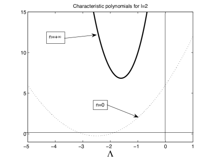
Figure 2. Illustrations to characteristic polynomials (3.8) for $n=+\infty$ and $n=0$; $l=2$.

5.2. Sharp estimates of $n^{*}_{l}$ for $l=2,3,4,5,10,100$

In order to get those saddle-node eigenvalue bifurcation points, we study numerically the characteristic equation (3.9) for $n>0$. In view of (3.13), we are not interested in the non-zero case $l=0$.

Again, by (3.13), for $l=1$, we see that, for any $n>0$, there exists

$$\Lambda_{1}(n)=-1.$$

However, for any arbitrarily large $n>0$, there exists another eigenvalue $\hat{\Lambda}_{1}(n)$ shown in Figure 3. It is interesting that, starting at the bifurcation value

$$\hat{\Lambda}_{1}(0)=-l-1=-2,\quad\hbox{precisely at}\quad\hat{n}^{*}=\frac{1}{2},$$

the value of $\hat{\Lambda}_{1}(n)$ crosses -1 and remains existent. Indeed, one can see from the characteristic equation (3.9) that

(5.4) $$\textstyle{l=1:\quad\mbox{there exists the double root}\,\,\,\hat{\Lambda}_{1}(n)=\Lambda_{1}(n)=-1,\,\,\,\mbox{iff}\,\,\,n=\frac{1}{2}.}$$

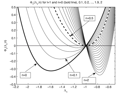
Figure 3. Graph of the characteristic polynomial (3.13) for $l=1$ and various values of $n=0,0.1,...,1.9,2$.

For $l=2$, the situation is different: Figure 4 clearly shows existence of the saddle-node bifurcation at some $n_{2}^{*}\in(0.1,0.2)$. More accurate numerics give the following estimates of these bifurcation points and the corresponding coinciding eigenvalues:

(5.5) $$0.11912<n_{2}^{*}<0.11913,\quad\mbox{where}\quad\Lambda_{2}(n_{2}^{*})=-2.4782...\,,$$

so that, for $n>n^{*}_{2}$, there are no real eigenvalues of (3.13).

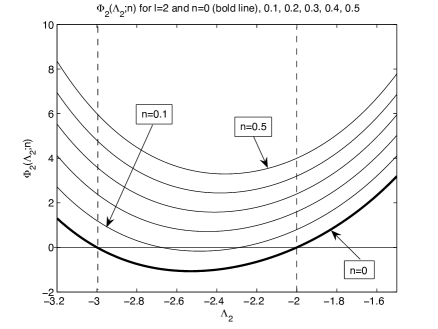
Figure 4. Graph of the characteristic polynomial (3.13) for $l=2$ and various values of $n=0,0.1,0.2,0.3,0.4,0.5$.

Furthermore, Figures 5 and 6 show similar bifurcation phenomena for $l=3$ and $l=4$ respectively. The bifurcation points and eigenvalues satisfy:

(5.6) $$\begin{matrix}n_{3}^{*}=0.052292...,\,\,\,\Lambda_{3}(n_{3}^{*})=-3.546...\vskip 3.0pt plus 1.0pt minus 1.0pt\\ \quad\mbox{and}\quad n_{4}^{*}=0.025354...,\,\,\,\Lambda_{4}(n_{4}^{*})=-4.55514....\,.\end{matrix}$$

We expect that, for larger $l$, bifurcation values become even smaller. For instance, our numerical estimates of the next bifurcation point and coinciding (double) eigenvalues for $l=5$ are:

(5.7) $$n_{5}^{*}=0.014859,\quad\mbox{where}\quad\Lambda_{5}(n^{*}_{5})=-5.546...\,.$$

Finally, we take larger $l=10$ and $l=100$:

(5.8) $$\begin{matrix}n_{10}^{*}=0.0036245...\,,\,\,\,\Lambda_{10}(n_{10}^{*})=-10.5254...\vskip 3.0pt plus 1.0pt minus 1.0pt\\ \quad\mbox{and}\quad n_{100}^{*}=0.00002555062...\,,\,\,\,\Lambda_{10}(n_{10}^{*})=-100.5025...\,.\end{matrix}$$

We see that, for $l=100$, the bifurcation-turning point of eigenvalues $n$-branches occurs already at very small $n\sim 10^{-5}$, implying the following final remarks naturally touching the cases $n>n_{l}^{*}$.

5.3. Problem of regularity at boundary points for nonlinear problems

It should be mentioned that the problem of regularity at boundary points has been studied before using the so-called Wiener’s regularity test/criterion via concepts of potential-theoretic Bessel (Riesz) capacities to strongly elliptic equations. In that sense the problem is formulated in terms of a divergence series of capacities, measuring the thickness of the complement of the domain near the point of the boundary at which the regularity is analysed (in this case the origin 0); see [8] for en extensive history of this problem applied to elliptic and parabolic equations, and the Kozlov–Maz’ya–Rossmann’s monographs [17, 18] for just elliptic problems.

Therefore, following those arguments the principal extension of Wiener’s-like capacity regularity test to a nonlinear degenerate $p$-Laplacian operator, with $p\in(1,N]$ was due to Maz’ya in 1970 [21], who extended it later on to have a sufficient capacity regularity condition to be optimal for any $p>1$.

Note that the analysis of this kind of problem was completed for second order elliptic and parabolic equations by Wiener (1924) for the Dirichlet problem in [25] and Petrovskii (1934), and extended in the 1960’s-1970’s for $2m$th-order PDEs by Kondriat’ev [15] and Maz’ya [21, 22]. The key question was always to determine the optimal, and as sharp as possible, conditions on the “shape” of the continuous boundary under which the solutions is continuous at the boundary points.

Thus, one of the approaches was to treat the problem at the singular boundary point by blow-up evolution via approaching this “singular” boundary point. Then, the rescaled pencil operators seem to be key. In that respect even though Konfriat’ev’s paper was not devoted to regularity issues, it represented a novel idea and involved the use of spectral properties of pencil operators, such as those we have used here, for describing the asymptotics of solutions near singularity boundary points assuming a kind of “elliptic evolution” approach for elliptic problems.

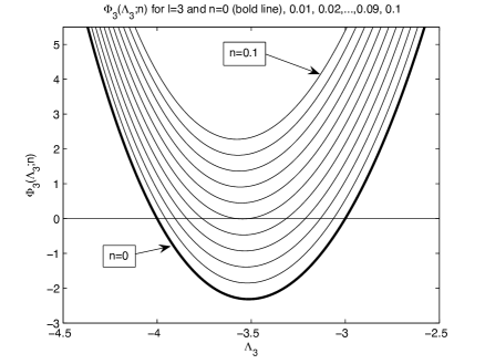
Figure 5. Graph of the characteristic polynomial (3.13) for $l=3$ and various values of $n=0,0.01,...,0.1$.

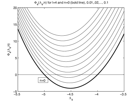
Figure 6. Graph of the characteristic polynomial (3.13) for $l=4$ and various values of $n=0,0.001,...,0.01$.

5.4. Final comment on zeros for the $p$-Laplacian

In this connection, it is important to mention that, for nonlinear problems, “blow-up” structures (at present, “blow-up” zero structures) may be of different forms, especially, for the $p$-Laplace operators. For instance, in [4], it was shown that blow-up in a quasilinear Frank–Kamenetskii equation from combustion theory (a solid fuel model for $n=0$),

(5.9) $$u_{t}=(|u_{x}|^{n}u_{x})_{x}+{\mathrm{e}}^{u},\quad n>0,$$

there exists an infinite sequence of critical exponents

$$\{n_{k}\}\to n_{\infty}<\infty,$$

so that the overall number of blow-up self-similar solutions changes by 1 when $n$ crosses each critical $n_{k}$. Recall that, for $n=0$, i.e., for the classic Frank–Kamenetskii equation from the 1930s, no such self-similar solutions exist at all, i.e., the above is a nonlinear phenomenon associated with the $p$-Laplace diffusion.

Let us add that this phenomenon is associated with the increase of rotations on a phase plane admitted by ODEs for blow-up profiles, so that, for

$$n>n_{\infty},$$

there exist very complicated families of solutions, including those having infinite number of oscillations about a constant equilibrium; see also [11]. In other words, e.g., for sufficiently small

$$0<n<n_{1},$$

there exists a single “nonlinear” blow-up structure, while all others (a countable family) can be obtained via linearization and matching, i.e., these are closer to similar blow-up behaviour for $n=0$. For

$$n_{2}<n<n_{3},$$

there are two self-similar profiles (the rest are linearized), etc.

Similarly, in our nodal set case (3.4) completely coincides with the linear representation, but until some maximal critical value $n_{*}^{l}$. We do not know, whether, for $n>n_{*}^{l}$ there exist other types of “nonlinear multiple zeros” at $\tau=+\infty$ for the evolution equation (3.3). Though, bearing in mind the finite propagation property of the $p$-Laplacian in the evolution sense and its infinitely oscillatory properties from [4, 11] for large exponents (also, a 2D problem, in the rescaled variables $\{z,\tau\}$, with $\tau=-\ln(T-t)$, cf. $\tau$ in (2.1), similar to (3.3)), we can expect some complicated non-self-similar zero structures of nodal sets that makes the evolution completeness problem of multiple zeros extremely difficult. Nevertheless, an “accidental” 1-homogeneity (existence of an “linear” invariant scaling) of (3.3) could make it slightly easier.

6. Towards $p$-bi-Laplace equation

Consider briefly (1.11). Using the same rescaled variables (2.1) and bearing in mind the corresponding $(z,\tau)$-representation (2.2) of the Laplacian, we arrive at the equation

(6.1) $$\Delta_{(z,\tau)}(|\Delta_{(z,\tau)}w|^{n}\Delta_{(z,\tau)}w)=0.$$

Next, performing all the technical computations, using the homogeneity of the final elliptic equation (recall the symmetry $w\mapsto Cw$, $C\in\mathbb{R}$, of (6.1)), we are looking for solutions via nonlinear eigenfunctions (3.4), for which

$$D_{\tau}=\Lambda I,$$

to get the corresponding nonlinear eigenvalue problem. The latter, for $n=0$, reduces to that for the bi-Laplacian one [3], which is shown to admit four families of harmonic polynomials as eigenfunctions of a quadratic pencil of non self-adjoin operators. This allows:

(i) to derive a nonlinear (polynomial) characteristic equation using the same assumption on the polynomial growth at infinity (associated with the analyticity of solutions of this ODE away from degeneracy points);

(ii) to prove existence of nonlinear eigenfunctions for proper values of $\Lambda$;

(iii) to establish a proper branching of nonlinear eigenfunctions at $n=0$ from harmonic polynomials;

(iv) to study, both analytically and numerically, those saddle-node $n$-bifurcation points for eigenvalues;

etc.

In other words, these are quite similar to what we have done above for the $p$-Laplace equation, with more technical features, indeed.

References

- [1] R.A. Adams, Sobolev Spaces, Pure and Applied Mathematics, Vol. 65, Acad. Press, New York/London, 1975.
- [2] P. Álvarez-Caudevilla and V.A. Galaktionov, Local bifurcation-branching analysis of global and “blow-up” patterns for a fourth-order thin film equation, Nonlinear Differ. Equat. Appl., 18 (2011), 483–537.
- [3] P. Álvarez-Caudevilla and V.A. Galaktionov, Blow-up scaling and global behaviour of the solutions of the bi-Laplace equation in domains with a multiple crack section, submitted.
- [4] C. Budd and V. Galaktionov, Stability and spectra of blow-up in problems with quasi-linear gradient diffusivity, Proc. Roy. Soc. London A, 454 (1998), 2371–2407.
- [5] K. Deimling, Nonlinear Functional Analysis, Springer-Verlag, Berlin/Tokyo, 1985.
- [6] J. W. Dettman, Mathematical Methods in Physics and Engineering, Mc-Graw-Hill, New York, 1969.
- [7] D. Funaro, Polynomial Approximation of Differential Equations, Springer-Verlag, Berlin/Tokyo, 1992.
- [8] V.A. Galaktionov, On regularity of a boundary point for Higher-order Parabolic Equations: Towards Petrovskii-type criterion by blow-up approach, NoDEA Nonlinear Differential Equations Appl. 16, (2009), no. 5, 597–655.
- [9] V.A. Galaktionov, Geometric Sturmian Theory of Nonlinear Parabolic Equations and Applications, ChapmanHall/CRC, Boca Raton, Florida, 2004.
- [10] V.A. Galaktionov, Evolution completeness of separable solutions of nonlinear diffusion equations in bounded domains, Math. Meth. Appl. Sci., 27 (2004), 1755-1770.
- [11] V.A. Galaktionov, S.P. Kurdyumov, S.A. Posashkov, and A.A. Samarskii, A nonlinear elliptic problem with a complex spectrum of solutions, USSR Comput. Math. Math. Phys., 26 (1986), 48–54.
- [12] J. Hadamard, Lectures on Cauchy’s problem in linear partial differential equations. Dover Publications, New York, 1953. iv+316 pp.
- [13] A.N. Kolmogorov and S.V. Fomin, Elements of the Theory of Functions and Functional Analysis, Nauka, Moscow, 1976.
- [14] V.A. Kondrat’ev, Boundary value problems for parabolic equations in closed regions, Trans. Moscow Math. Soc., 15 (1966), 400–451.
- [15] V.A. Kondrat’ev, Boundary value problems for elliptic equations in domains with conical or angular points, Trans. Moscow Math. Soc., 16 (1967), 209–292.
- [16] M. Krein and H. Langer, On some mathematical principles in the linear theory of damped oscillations of continua. I, II, Int. Equat. Oper. Theory, 1 (1978), 364–399, 539–566.
- [17] V.A Kozlov, V.G. Maz’ya and J. Rossmann Elliptic Boundary Value Problems in Domains with Point Singularities, Math. Surveys Monogr., Vol. 52, Amer. Math. Soc., Providence, RI, 1997. (1976), 225–242.
- [18] V.A Kozlov, V.G. Maz’ya and J. Rossmann Spectral Problems with Corner Singularities of Solutions to Elliptic Problems, Math. Surveys Monogr., Vol. 85, Amer. Math. Soc., Providence, RI, 2001. (1976), 225–242.
- [19] A. Lemenant, On the homogeneity of global minimizers for the Mumford-Shah functional when is a smooth cone, Rend. Sem. Mat. Univ. Padova, 122 (2009), 129–159.
- [20] A.S. Markus, Introduction to Spectral Theory of Polynomial Operator Pencils, Translated from the Russian by H. H. McFaden. Translation edited by Ben Silver. With an appendix by M. V. Keldysh. Transl. of Math. Mon., 71, Amer. Math. Soc., Providence, RI, 1988.
- [21] V. Maz’ya, On the continuity at a boundary point of solutions of quasi-linear elliptic equations, Vestnik Leningr. Univ., Math. Mech. Actronom., 25 (1970), 42–55; English transl.: Vestnik Leningr. Univ. Math., 3 (1976), 225–242.
- [22] V. Maz’ya, Behaviour of solutions to the Dirichlet problem for the biharmonic operator at the boundary point, Equadiff IV (Proc. Czechoslovak Conf. Diff. Equat. Appl., Prague, 1977), Lecture Notes Math., Vol. 703, Springer, Berlin, 250–262.
- [23] D. Mumford and J. Shah, Optimal approximations by piecewise smooth functions and associated variational problems, Commun. Pure Appl. Math., 42 (1989), 577–685.
- [24] C. Sturm, Mémoire sur une classe d’équations à différences partielles, J. Math. Pures Appl., 1 (1836), 373–444.
- [25] N. Wiener, The Dirichlet problem, J. Math. and Phys. Mass. Inst. Tech., 3 (1924), 127–146; reprinted in: N. Wiener, Collected Works with Commentaries, Vol. I, ed. P. Masani, Mathematicians of Our Time, 10, MIT Press, Cambridge, Mass., 1976, 394–413.