Synthetic spin-orbit interactions and magnetic fields in ring-cavity QED

Abstract

The interactions between light and matter are strongly enhanced when atoms are placed in high-finesse quantum cavities, offering tantalizing opportunities for generating exotic new quantum phases. In this work we show that both spin-orbit interactions and strong synthetic magnetic fields result when a neutral atom is confined within a ring cavity, whenever the internal atomic states are coupled to two off-resonant counter-propagating modes. We diagonalize the resulting cavity polariton Hamiltonian and find characteristic spin-orbit dispersion relations for a wide range of parameters. An adjustable uniform gauge potential is also generated, which can be converted into a synthetic magnetic field for neutral atoms by applying an external magnetic field gradient. Very large synthetic magnetic fields are possible as the strength is proportional to the (average) number of photons in each of the cavity modes. The results suggest that strong-coupling cavity quantum electrodynamics can be a useful environment for the formation of topological states in atomic systems.

I Introduction

The spin-orbit interaction in solids is the coupling of an electron’s spin to its center-of-mass momentum, and is closely related to the spin-orbit coupling in atomic systems. In two-dimensional electron gases two kinds of spin-orbit coupling have important effects on the electronic band structure: Dresselhaus Dresselhaus (1955) and Rashba Bychkov and Rashba (1984) interactions. In a groundbreaking paper Kane and Mele (2005a), Kane and Mele showed that including a spin-orbit interaction in the Hamiltonian of graphene, while respecting all of the material’s symmetries, nevertheless opens up a band gap. The resulting bands become topologically nontrivial, so that the material supports a pair of robust conducting edge states characterized by a nontrivial $Z_{2}$ topological invariant Kane and Mele (2005b). This new phase of matter is known as a topological insulator, or a quantum spin Hall (QSH) insulator in two dimensions, and its discovery has opened up a fascinating new research area in condensed matter physics Hasan and Kane (2010). Determining the conditions under which topological states could arise in condensed matter systems is the subject of continuing investigations Schnyder et al. (2008); Wen (2012); Slager et al. (2013).

Ultracold atomic gases provide a rich environment for the simulation of condensed matter physics Jaksch and Zoller (2005); Lewenstein et al. (2007); Bloch et al. (2008). For example, interacting atoms confined in optical lattices experience a crystalline environment that can mimic strongly correlated superfluid and magnetic states. Over the past decade, many theoretical schemes have been proposed to generate synthetic gauge potentials for neutral ultracold atomic gases via atom-light interactions Dalibard et al. (2011). In recent years, both synthetic magnetic Lin et al. (2009) and electric Lin et al. (2011a) fields have been realized experimentally. The spin-orbit coupling can be interpreted as a non-Abelian gauge field Hatano et al. (2007), and Lin et al. recently realized a scheme to generate a combination of Rashba and Dresselhaus spin-orbit couplings in ultracold neutral atoms by means of resonant two-photon Raman transitions Lin et al. (2011b). The strength of the gauge field potentials in these experiments is limited by the atomic recoil momentum, though there are recent theoretical proposals that would push these to much higher values Moller and Cooper (2012); Baur and Cooper (2012); Cooper and Dalibard (2013).

Placing atoms in high-finesse optical cavities strongly enhances atom-photon interactions Walther et al. (2006), with numerous potential applications to quantum information science Raimond et al. (2001). While much of the early work focused on single atoms, recent investigations of cavity quantum electrodynamics (QED) with multiple trapped ultracold atoms Colombe et al. (2007) are revealing fascinating new phenomena. The field mode to which atoms are collectively coupled is in turn affected by the atomic states, giving rise to cavity mediated long-range atom-atom interactions Ritsch et al. (2013). Other examples include the Dicke phase transition Baumann et al. (2010) and a collective atomic recoil laser Kruse et al. (2003); von Cube et al. (2004); Slama et al. (2007a, b) in many-atom linear and ring cavity QED, respectively.

The strong coupling of cavity QED therefore offers the tantalizing prospect of enhancing the magnitude of synthetic gauge fields and spin-orbit interactions in atomic systems, as well as inducing unique strongly correlated states of both atoms and photons with no analog in condensed matter systems. In this work, we show how to simultaneously engineer a spin-orbit interaction and a synthetic magnetic field for a single neutral atom confined inside a ring cavity, as a first step toward generating topological states in ultracold atomic systems. We build on the central ideas of two-photon resonant Raman transitions described in Ref. Lin et al. (2011b), in which absorption and re-emission of photons from one beam to the other naturally couples the atom’s internal states to their center-of-mass momentum. Two propagating modes of a high-finesse ring cavity accomplish the same purpose, but with an enhanced atom-photon coupling strength. This potential advantage comes at the cost of increased mathematical complexity, because unlike the continuum Raman case both the atom and photon degrees of freedom need to be treated fully quantum mechanically.

The calculations presented here reveal that the spin-orbit interactions and synthetic magnetic fields emerge naturally as the limits of zero two-photon detuning between the atomic and cavity frequencies and large two-photon detuning, respectively. The spin-orbit interactions are only weakly dependent on the occupation of the cavity modes, and in fact are robust already at the level of a few photons. That said, the energy barrier between the energy levels split by the spin-orbit interactions is greatest when the difference between the occupation of the two modes is largest. In principle, this parameter is adjustable experimentally Brattke et al. (2001); McKeever et al. (2004); Keller et al. (2004); Cooper et al. (2013). The strength of the synthetic magnetic fields is proportional to the square of the total number of photons in the cavity. The cavity QED environment therefore promises huge synthetic magnetic fields, potentially much larger than are currently accessible to ultracold atom experiments. The readiness with which spin-orbit interactions and synthetic magnetic fields are manifested in cavity QED should facilitate the production of new strongly correlated states in these systems.

The manuscript is organized as follows. The model of the atom interacting with a ring cavity is described in Sec. II, and the governing Hamiltonian is derived. In Sec. III, this Hamiltonian is expressed in terms of polaritons and diagonialized to obtain the spectrum of excitations. Sec. IV describes the circumstances under which synthetic spin-orbit interactions and magnetic fields emerge in this model. Sec. V discusses the results with a view toward future calculations.

II Model and Hamiltonian

Consider a ring cavity with two counter-propagating modes $a_{1}e^{\imath k_{1}z}$ and $a_{2}e^{-\imath k_{2}z}$, where $a_{i}$ are field annihilation operators for the photon and $k_{i}=\omega_{i}/c$ are the photon wavenumber expressed in terms of their frequencies $\omega_{i}$. Note that in this work $\imath\equiv\sqrt{-1}$. Three atomic levels are coupled via these two cavity modes in the $\Lambda$ scheme, as depicted in Fig. 1. The states $\left|a\right>$, $\left|b\right>$, and $\left|e\right>$ are arbitrary internal states of an atom whose energies satisfy the relations $E_{e}>E_{b}>E_{a}$ and $\{E_{ea},E_{eb}\}\gg E_{ba}$, where $E_{ij}\equiv E_{i}-E_{j}$. For example, the states $\left|a\right>$ and $\left|b\right>$ might be energy levels in the same hyperfine manifold with an energy separation on the order of MHz while the state $\left|e\right>$ could be an excited electronic level with an energy separation on the order of THz. The mode $a_{1}e^{\imath k_{1}z}$ ($a_{2}e^{-\imath k_{2}z}$) propagates to the right (left) and couples solely to the $\left|a\right>\leftrightarrow\left|e\right>$ ($\left|b\right>\leftrightarrow\left|e\right>$) transition.

The Hamiltonian in the rotating-wave approximation reads

$$H = \frac{\hbar^{2}q_{z}^{2}}{2m}I_{3\times 3}+E_{a}\sigma_{aa}+E_{b}\sigma_{bb}+E_{e}\sigma_{ee}$$ (1)

$$+ \hbar(\omega_{1}a^{\dagger}_{1}a_{1}+\omega_{2}a_{2}^{\dagger}a_{2})$$

$$+ \hbar\left(g_{ae}(z)a_{1}\sigma_{ea}+g_{be}(z)a_{2}\sigma_{eb}+\mbox{H.c.}\right),$$

where $\sigma_{ij}=\left|i\right>\left<j\right|$, $g_{ae}(z)=g_{ae}e^{\imath k_{1}z}$, $g_{be}(z)=g_{be}e^{-\imath k_{2}z}$ and H.c. stands for Hermitian conjugate. Here $\hbar q_{z}$ is the center-of-mass momentum of the atom and $I_{3\times 3}$ is the identity matrix in the internal atomic state space. Note that strictly speaking, Eq. (1) is the Hamiltonian density; alternatively it can be considered the Hamiltonian with an implied sum over $q_{z}$. To a first approximation, this Hamiltonian represents an atom with infinite excited-state lifetime and an exceptionally high-finesse cavity, neglecting atomic spontaneous emission and cavity losses by mirror leakage, as well as gains by external pumps. Even with these simplifying assumptions, the analysis of this Hamiltonian is quite involved as can be seen below; relaxing these assumptions will therefore be the focus of future work.

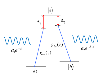
Figure 1: Two low-lying atomic levels $\left|a\right>$ and $\left|b\right>$ are coupled in the $\Lambda$ scheme to an excited state $\left|e\right>$ by two counter-propagating cavity modes $a_{1}e^{\imath k_{1}z}$ and $a_{2}e^{-\imath k_{2}z}$ with strength $g_{ae}(z)$ and $g_{be}(z)$, respectively. The transitions are detuned from resonance by $\Delta_{1}$ and $\Delta_{2}$.

If the cavity modes are far off-resonance from atomic transitions then the adiabatic condition holds. That is, if the frequency detunings $\hbar\Delta_{1}\equiv\hbar\omega_{1}-E_{ea}$ and $\hbar\Delta_{2}\equiv\hbar\omega_{2}-E_{eb}$ are very large compared to $E_{ba}$ then the excited state $\left|e\right>$ can be adiabatically eliminated Gerry and Eberly (1990). Details of the procedure can be found in the Appendix A. The effective Hamiltonian for the ground pseudospin states $\left|a\right>$ and $\left|b\right>$ and the cavity modes then becomes

$$H_{\rm eff} = \frac{\hbar^{2}q_{z}^{2}}{2m}I_{2\times 2}+\frac{1}{2}\hbar\tilde{\omega}_{0}\sigma_{z}+\hbar(\omega_{1}a^{\dagger}_{1}a_{1}+\omega_{2}a_{2}^{\dagger}a_{2})$$ (2)

$$+ \hbar\Omega_{R}\left(e^{\imath(k_{1}+k_{2})z}a_{2}^{\dagger}a_{1}\sigma_{ba}+\mbox{H.c.}\right),$$

where $\sigma_{z}=|b\rangle\langle b|-|a\rangle\langle a|$, and $\hbar\tilde{\omega}_{0}=\tilde{E}_{b}-\tilde{E}_{a}>0$. The $\tilde{E}_{i}$ correspond to the AC Stark-shifted atomic energies (LABEL:ACStark). The $I_{2\times 2}$ operator is the identity matrix in the ground pseudospin state space, and will be implied in the remainder of this work. The two-photon Rabi frequency (45) is given by $\Omega_{R}=g_{ae}g_{be}\left(\frac{\Delta_{1}+\Delta_{2}}{\Delta_{1}\Delta_{2}}\right)$ under the assumption that $\{g_{ae},g_{be}\}\in\Re$.

It is useful to perform a Galilean transformation of this Hamiltonian into the frame moving at the momentum transferred to the atom by the interaction with the photons. This is accomplished using the unitary operator $U=\exp{[\imath(k_{1}\sigma_{aa}-k_{2}\sigma_{bb})z]}$:

$$\tilde{H}_{\rm eff}\equiv UH_{\rm eff}U^{\dagger} = \frac{\hbar^{2}}{2m}[q_{z}-(k_{1}\sigma_{aa}-k_{2}\sigma_{bb})]^{2}$$ (3)

$$+ \frac{1}{2}\hbar\tilde{\omega}_{0}\sigma_{z}+\hbar(\omega_{1}a_{1}^{\dagger}a_{1}+\omega_{2}a_{2}^{\dagger}a_{2})$$

$$+ \hbar\Omega_{R}\left(a_{2}^{{\dagger}}a_{1}\sigma_{ba}+\mbox{H.c.}\right),$$

where $U\sigma_{ba}U^{{\dagger}}=e^{-\imath(k_{1}+k_{2})z}\sigma_{ba}$ using the Baker-Campbell-Hausdorff formula. One could have applied the unitary transformation $U^{\prime}=\exp{[\imath(k_{1}a_{1}^{\dagger}a_{1}-k_{2}a_{2}^{\dagger}a_{2})z]}$ instead; although the first term of the resulting Hamiltonian will be different from that given above, the final results discussed below are independent of the particular choice of a unitary transformation. The last term in Eq. (3) resembles the interaction term in the Jaynes-Cummings model Shore and Knight (1993), but the $a$ is replaced by a two-photon $a_{2}^{{\dagger}}a_{1}$ operator.

In order to reveal the underlying symmetries of the Hamiltonian (3), it is useful to express the operators in the Schwinger representation. Let $\sigma_{+}=\sigma_{ba}=\frac{1}{2}(\sigma_{x}+\imath\sigma_{y})=\frac{1}{\hbar}(s_{x}+\imath s_{y})=\frac{1}{\hbar}s_{+}$ and $\sigma_{-}=\sigma_{ab}=\frac{1}{\hbar}s_{-}$ be the raising and lowering operators for the atom, and $\frac{2}{\hbar}s_{z}=\sigma_{z}=\sigma_{+}\sigma_{-}-\sigma_{-}\sigma_{+}=|b\rangle\langle b|-|a\rangle\langle a|$. If there are only exactly two modes of the cavity and $\omega_{1}>\omega_{2}$, one can make use of the Schwinger angular momentum operators Biedenharn and Dam (1965) for the photon field operators $j_{x}=\frac{\hbar}{2}(a_{1}^{\dagger}a_{2}+a_{2}^{\dagger}a_{1})$, $j_{y}=\frac{\hbar}{2\imath}(a_{1}^{\dagger}a_{2}-a_{2}^{\dagger}a_{1})$, and $j_{z}=\frac{\hbar}{2}(a_{1}^{\dagger}a_{1}-a_{2}^{\dagger}a_{2})$, which satisfy the $SU(2)$ Lie algebra (or angular momentum commutation relation)

$$[j_{n},j_{m}]=\imath\hbar\varepsilon^{nml}j_{l},$$ (4)

where $\varepsilon^{nml}$ is the totally antisymmetric tensor. As in the atomic case, one can define photonic angular-momentum raising and lowering operators $j_{+}=j_{x}+\imath j_{y}=\hbar a_{1}^{\dagger}a_{2}$ and $j_{-}=j_{x}-\imath j_{y}=\hbar a_{2}^{\dagger}a_{1}$. The Hamiltonian (3) can then be recast as

$$\tilde{H}_{\rm eff} = \frac{\hbar^{2}}{2m}\left\{q_{z}I_{2\times 2}-\left[\frac{\Delta k}{2}I_{2\times 2}-k\sigma_{z}\right]\right\}^{2}$$ (5)

$$+ \tilde{\omega}_{0}s_{z}+\frac{\hbar}{2}(\omega_{1}+\omega_{2})N+(\omega_{1}-\omega_{2})j_{z}$$

$$+ \frac{\Omega_{R}}{\hbar}(j_{-}s_{+}+j_{+}s_{-}),$$

where $k=(k_{1}+k_{2})/2$, $\Delta k=k_{1}-k_{2}$ and $I_{2\times 2}=\sigma_{aa}+\sigma_{bb}$ as before. Here, $N=a_{1}^{\dagger}a_{1}+a_{2}^{\dagger}a_{2}$ is the total photon number operator with eigenvalues $n=2j$, where $\hbar^{2}j(j+1)$ is the eigenvalue of the total photon spin operator $\mathbf{j}^{2}$.

The first term in the Hamiltonian (5) strongly resembles spin-orbit coupling, with equal contributions of Dresselhaus Dresselhaus (1955) and Rashba Bychkov and Rashba (1984) terms. Expanding the quadratic operator provides a cross term that explicitly couples the linear momentum to the pseudospin degree of freedom. A more formal mapping will be discussed in detail in the next section.

Aside from the first term, the Hamiltonian (5) corresponds to a generalized Jaynes-Cummings model:

$$H_{\rm GJC} = \tilde{\omega}_{0}s_{z}+\frac{\hbar}{2}(\omega_{1}+\omega_{2})N+(\omega_{1}-\omega_{2})j_{z}$$ (6)

$$+ \frac{\Omega_{R}}{\hbar}(j_{-}s_{+}+j_{+}s_{-}).$$

The components of $\mathbf{j}$ and $\mathbf{s}$ both satisfy the angular momentum commutation relation (4), so one can define the total angular momentum operator $\mathbf{J}=\mathbf{j}+\mathbf{s}$. Because $[H_{\rm GJC},N]=[H_{\rm GJC},\mathbf{j}^{2}]=[H_{\rm GJC},J_{z}]=0$, it is conventional to represent the eigenstates of $H_{\rm GJC}$ and $\tilde{H}_{\rm eff}$ in a basis labeled by the eigenstates of $s_{z}$, $j_{z}$, and ${\bf j}$, with eigenvalues $\hbar m_{s}=\pm\hbar/2$, $\hbar m_{j}\equiv\hbar(n_{1}-n_{2})/2$, and $\hbar j=(\hbar/2)(n_{1}+n_{2})=(\hbar/2)n$, respectively. For reasons described in detail below, it turns out to be more convenient to instead express the basis in eigenstates of ${\bf j}$, $s_{z}$, and $J_{z}$, where the eigenvalues of the last quantity $\hbar m_{z}=\hbar(m_{j}+m_{s})=(\hbar/2)(n_{1}-n_{2}\pm 1)$. Note that the only component of the total angular momentum operator ${\bf J}$ that commutes with $\tilde{H}_{\rm eff}$ is $J_{z}$. Thus, the symmetry of the spin space of the Hamiltonian is reduced to $U(1)$.

III Polariton Mapping

While the first part of the effective Hamiltonian (5) indicates that the atoms experience an effective spin-orbit coupling through their interactions with the cavity modes, the remainder corresponds to a generalized Jaynes-Cummings model. The natural representation of the quasiparticles in the latter model is that of cavity polaritons (superpositions of atomic and photonic excitations). Explicit diagonalization of the full polariton Hamiltonian, performed below, shows that in fact it is the dressed pseudospin states that experience the spin-orbit interactions and synthetic magnetic fields.

III.1 Diagonalizing the generalized Jaynes-Cummings Hamiltonian

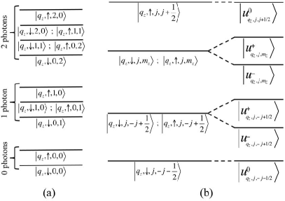
Figure 2: The energy manifolds of the atom-cavity system in the uncoupled $q_{z}$, $s_{z}$, $N_{1}$, and $N_{2}$ basis (i.e. $\left|q_{z},\uparrow\downarrow,n_{1},n_{2}\right>$) are shown in (a). Shown in (b) is the $2j$-photon manifold and the corresponding sub-manifolds in the uncoupled $q_{z}$, $s_{z}$, $\mathbf{j}$, and $J_{z}$ basis (i.e. $\left|q_{z},\downarrow\uparrow,j,m_{z}\right>$), and the resulting dressed states of Eq. (11) within the manifold. Note that here $\delta=0$.

In order to map the Hamiltonian (5) into the polariton basis, we first exactly diagonalize $H_{\rm GJC}$. Ignoring the atom-photon coupling $j_{+}s_{-}+j_{-}s_{+}$ term, the natural basis states can be represented by $\left|q_{z}\right>\otimes\left|\downarrow\uparrow\right>\otimes\left|n_{1}\right>\otimes\left|n_{2}\right>=\left|q_{z},\downarrow\uparrow,n_{1},n_{2}\right>$, where $\left|\downarrow\right>=|a\rangle$, $\left|\uparrow\right>=|b\rangle$, and $n_{1}$ and $n_{2}$ are the number of photons in the first and second cavity modes, respectively. With a total of $n$ photons in the cavity, there are $2(n+1)$ basis states for each value of $q_{z}$. These states are depicted in Fig. 2. For example, the states for $n=1$ correspond to $\left|q_{z},\downarrow,0,1\right>$, $\left|q_{z},\downarrow,1,0\right>$, $\left|q_{z},\uparrow,0,1\right>$, and $\left|q_{z},\uparrow,1,0\right>$. The $j_{+}s_{-}+j_{-}s_{+}$ term couples basis states $\left|q_{z},\downarrow,n_{1},n_{2}\right>$ and $\left|q_{z},\uparrow,n_{1}-1,n_{2}+1\right>$ together within a given $n$ manifold, but the states $\left|q_{z},\downarrow,0,n\right>$ and $\left|q_{z},\uparrow,n,0\right>$ will remain uncoupled. For each value of $n$, the Hamiltonian therefore block diagonalizes into $n+2$ distinct blocks, of which $n$ are two-dimensional and two are one-dimensional.

Following the discussion in the previous section, it is convenient to represent the basis states above in terms of pseudospin quantum numbers: $\left|q_{z},\downarrow\uparrow,j,m_{z}\right>=\left|q_{z}\right>\otimes\left|\downarrow\uparrow\right>\otimes\left|j,m_{z}\right>$, where $\hbar j=\hbar n/2$ and $\hbar m_{z}=\hbar(m_{j}+m_{s})=\frac{\hbar}{2}(n_{1}-n_{2}\pm 1)$ with $m_{z}=-j-\frac{1}{2},\ldots,j+\frac{1}{2}$. In this representation, the states $\left|q_{z},\downarrow,j,-j-\frac{1}{2}\right>\equiv\left|u^{0}_{q_{z},j,-j-\frac{1}{2}}\right>$ and $\left|q_{z},\uparrow,j,j+\frac{1}{2}\right>\equiv\left|u^{0}_{q_{z},j,j+\frac{1}{2}}\right>$ are independent of the others, and have energies

$$E^{0}_{j,-j-\frac{1}{2}} = -\frac{\hbar\tilde{\omega}_{0}}{2}+\hbar\omega_{2}n_{2}=-\frac{\hbar\tilde{\omega}_{0}}{2}+2\hbar\omega_{2}j;$$

$$E^{0}_{j,j+\frac{1}{2}} = \frac{\hbar\tilde{\omega}_{0}}{2}+\hbar\omega_{1}n_{1}=\frac{\hbar\tilde{\omega}_{0}}{2}+2\hbar\omega_{1}j.$$ (7)

The remaining $2n$ states couple in pairs keeping $m_{z}$ fixed. For example, states with $m_{j}=\frac{1}{2}(n_{1}-n_{2})$ and $m_{s}=-\frac{1}{2}$ (atomic state $\left|\downarrow\right>=\left|a\right>$) couple with states with $m_{j}^{\prime}=\frac{1}{2}(n_{1}^{\prime}-n_{2}^{\prime})=\frac{1}{2}[(n_{1}-1)-(n_{2}+1)]=m_{j}-1$ and $m_{s}=+\frac{1}{2}$; both these have $m_{z}=\frac{1}{2}(n_{1}-n_{2}-1)=m_{j}-\frac{1}{2}$. The two-dimensional blocks of the Hamiltonian $H_{\rm GJC}$ are therefore

$$H_{\rm GJC}^{j,m_{z}} = \begin{pmatrix}\frac{\hbar\tilde{\omega}_{0}}{2}+\hbar\omega_{1}(n_{1}-1)+\hbar\omega_{2}(n_{2}+1)&\hbar\Omega_{R}\sqrt{n_{1}\left(n_{2}+1\right)}\cr\hbar\Omega_{R}\sqrt{n_{1}\left(n_{2}+1\right)}&-\frac{\hbar\tilde{\omega}_{0}}{2}+\hbar\omega_{1}n_{1}+\hbar\omega_{2}n_{2}\end{pmatrix}$$ (8)

$$= \hbar\left[\left(\omega_{1}+\omega_{2}\right)j+\left(\omega_{1}-\omega_{2}\right)m_{z}\right]I_{2\times 2}+\frac{\hbar}{2}\begin{pmatrix}-\delta&\Omega_{R}\sqrt{(2j+1)^{2}-4m_{z}^{2}}\cr\Omega_{R}\sqrt{(2j+1)^{2}-4m_{z}^{2}}&\delta\cr\end{pmatrix},$$

where the two-photon detuning is defined to be $\delta\equiv\left(\omega_{1}-\omega_{2}\right)-\tilde{\omega}_{0}\approx\Delta_{1}-\Delta_{2}$ and the number of photons in each mode is written in terms of the pseudospin quantum numbers as $n_{1}=j+m_{z}+\frac{1}{2}$, and $n_{2}=j-m_{z}-\frac{1}{2}$. Defining

$$\Delta_{j,m_{z}}\equiv\sqrt{\Omega_{R}^{2}\left[(2j+1)^{2}-4m_{z}^{2}\right]+\delta^{2}},$$ (9)

the eigenvalues of the two-dimensional blocks (8) are

$$E^{\pm}_{j,m_{z}}=\hbar[(\omega_{1}+\omega_{2})j+(\omega_{1}-\omega_{2})m_{z}]\pm\frac{\hbar\Delta_{j,m_{z}}}{2}.$$ (10)

Defining the mixing angle $\theta_{j,m_{z}}\equiv\cos^{-1}(-\delta/\Delta_{j,m_{z}})$, the dressed states (or polariton states) can be written

$$\begin{pmatrix}\left|u^{+}_{q_{z},j,m_{z}}\right\rangle\cr\vskip 2.84544pt\cr\left|u^{-}_{q_{z},j,m_{z}}\right\rangle\cr\end{pmatrix}=\begin{pmatrix}\cos\frac{\theta_{j,m_{z}}}{2}&\sin\frac{\theta_{j,m_{z}}}{2}\cr\vskip 2.84544pt\cr-\sin\frac{\theta_{j,m_{z}}}{2}&\cos\frac{\theta_{j,m_{z}}}{2}\cr\end{pmatrix}\begin{pmatrix}|q_{z},\uparrow,j,m_{z}\rangle\cr\vskip 2.84544pt\cr|q_{z},\downarrow,j,m_{z}\rangle\cr\end{pmatrix}.$$ (11)

Note that this treats $\tilde{\omega}_{0}$ and therefore $\delta$ as a constant independent of $j$ and $m_{z}$, which is not strictly correct. Using results found in the Appendix, the Stark-shifted atomic transition frequency is

$$\tilde{\omega}_{0} = \omega_{0}+\frac{2g_{be}^{2}}{\Delta_{2}}\left(j-m_{z}\right)-\frac{2g_{ae}^{2}}{\Delta_{1}}\left(j+m_{z}+1\right)$$ (12)

$$= \omega_{0}-\frac{2g_{ae}^{2}}{\Delta_{1}}+2j\left(\frac{g_{be}^{2}}{\Delta_{2}}-\frac{g_{ae}^{2}}{\Delta_{1}}\right)$$

$$- 2m_{z}\left(\frac{g_{ae}^{2}}{\Delta_{1}}+\frac{g_{be}^{2}}{\Delta_{2}}\right)$$

where $\omega_{0}=(E_{b}-E_{a})/\hbar$. The terms proportional to $j$ and $m_{z}$ can be ignored to a first approximation. While $2j=n$ is a large number when many photons occupy both modes, for a judicious choice of levels one should be able to ensure that $g_{be}^{2}/\Delta_{2}\approx g_{ae}^{2}/\Delta_{1}$. Likewise, $m_{z}=(n_{1}-n_{2}-1)/2$, which should be small if $n_{1}\sim n_{2}$. Thus $\tilde{\omega}_{0}\approx\omega_{0}-2g_{ae}^{2}/\Delta_{1}$ for each block. In fact, as shown below, synthetic magnetic fields are maximized when $n_{1}\sim n_{2}$. Even if $m_{z}$ is not small, for sufficiently big frequency detunings $\Delta_{i}$, the second and the last term in Eq. (12) will be negligible and $\tilde{\omega}_{0}\approx\omega_{0}$. Yet the important off-diagonal term in the $2\times 2$ Hamiltonian blocks (8) will remain appreciable as long as $j\gg m_{z}$.

The generalized Jaynes-Cummings Hamiltonian $H_{\rm GJC}$ is now diagonal in the dressed state basis

$$H_{\rm GJC}=\sum_{j,m_{z},\tau}E_{j,m_{z}}^{\tau}P_{j,m_{z},\tau}^{\dagger}P_{j,m_{z},\tau},$$ (13)

where $j=0,\frac{1}{2},1,\frac{3}{2},\ldots$, $m_{z}=-j-\frac{1}{2},\ldots,j+\frac{1}{2}$ in integer steps, and $\tau=\{0,\pm\}$. The energies $E^{\tau}_{j,m_{z}}$ are defined in Eqs. (7) and (10). The polariton field creation operator is defined as (c.f. Ref. Angelakis et al. (2007); Koch and Hur (2009))

$$P_{j,m_{z},\tau}^{\dagger}=\left|u_{q_{z},j,m_{z}}^{\tau}\right>\left<u_{q_{z},0,-1/2}^{0}\right|,$$ (14)

where the dependence of the field operator on $q_{z}$ is suppressed for convenience.

III.2 Diagonalizing the full Hamiltonian

We are now in a position to obtain the matrix elements of the full Hamiltonian (5) in the dressed-state basis. It suffices to obtain the coefficients

$$t^{\tau\tau^{\prime}}_{j,m_{z}}=k\left<u^{\tau}_{q_{z},j,m_{z}}\right|\sigma_{z}\left|u^{\tau^{\prime}}_{q_{z},j,m_{z}}\right>,$$ (15)

which are

$$t_{j,m_{z}}^{\pm\pm}=\pm k\cos\theta_{j,m_{z}};$$

$$t_{j,m_{z}}^{\pm\mp}=-k\sin\theta_{j,m_{z}};$$

$$t^{00}_{j,j+\frac{1}{2}}=-t^{00}_{j,-j-\frac{1}{2}}=k.$$ (16)

With Eqs. (7), (10), (13) and (15) and some straightforward algebra, the total Hamiltonian (5) becomes:

$$\tilde{H}_{\rm eff} = \sum_{j,m_{z}}\Bigg{[}\frac{\hbar^{2}}{2m}\Big{(}\tilde{q}_{z}+\sum_{\tau,\tau^{\prime}}t^{\tau\tau^{\prime}}_{j,m_{z}}P^{{\dagger}}_{j,m_{z},\tau}P_{j,m_{z},\tau^{\prime}}\Big{)}^{2}$$ (17)

$$+ \sum_{\tau}E^{\tau}_{j,m_{z}}P^{{\dagger}}_{j,m_{z},\tau}P_{j,m_{z},\tau}\Bigg{]}.$$

in the polariton basis. Here we have introduced the Doppler-shifted center-of-mass momentum $\tilde{q}_{z}\equiv q_{z}-\Delta k/2$. The second term in the square brackets can be considered as a Zeeman energy shift for each sub-manifold. The first term contains the essential feature of the spin-orbit interaction: a spin-dependent shift of the center-of-mass momentum. This can be made more explicit by introducing the effective spin operators

$$X_{j,m_{z}} \equiv P_{j,m_{z},+}^{{\dagger}}P_{j,m_{z},-}+P^{{\dagger}}_{j,m_{z},-}P_{j,m_{z},+};$$

$$Z_{j,m_{z}} \equiv P^{{\dagger}}_{j,m_{z},+}P_{j,m_{z},+}-P^{{\dagger}}_{j,m_{z},-}P_{j,m_{z},-},$$ (18)

whenever $m_{z}\neq\pm(j+1/2)$. The Hamiltonian (17) can then be written

$$\tilde{H}_{\rm eff}^{j,m_{z}} = \frac{\hbar^{2}}{2m}\Big{[}\tilde{q}_{z}I_{j,m_{z}}+k\cos\theta_{j,m_{z}}Z_{j,m_{z}}$$ (19)

$$- k\sin\theta_{j,m_{z}}X_{j,m_{z}}\Big{]}^{2}+\frac{\hbar\Delta_{j,m_{z}}}{2}Z_{j,m_{z}}$$

$$+ \hbar[(\omega_{1}+\omega_{2})j+(\omega_{1}-\omega_{2})m_{z}]I_{j,m_{z}},$$

for some arbitrary $j\neq 0$ and $m_{z}\neq\pm(j+1/2)$. This equation can be considered to be the main result of the present work. The term in brackets corresponds to the Hamiltonian of a particle with a Doppler-shifted center-of-mass momentum $\tilde{q}_{z}$ subject to a spin-dependent gauge field (i.e. the sign and strength of the guage field depends on the eigenstate of $m_{s}$). This takes a particularly simple form when $\cos\theta_{j,m_{z}}=0$, or zero two-photon detuning $\delta=0$. For this case, the kinetic energy term takes the usual spin-orbit form $(\hbar^{2}/2m)[\tilde{q}_{z}I_{j,m_{z}}-kX_{j,m_{z}}]^{2}$. The last term is an overall energy shift for each two-dimensional block labeled by $m_{z}$. The penultimate term can be considered as a Zeeman splitting for the dressed states.

Eq. (19) can be simplified slightly by defining $E_{R}\equiv\hbar^{2}k^{2}/2m$ as the atomic recoil energy and $p_{z}\equiv\tilde{q}_{z}/k$ as the Doppler-shifted center-of-mass momentum in units of $k$. Ignoring the constant shift for each submanifold labeled by $m_{z}$, one obtains

$$\frac{\tilde{H}_{\rm eff}^{j,m_{z}}}{E_{R}} = \Big{[}p_{z}I_{j,m_{z}}+\cos\theta_{j,m_{z}}Z_{j,m_{z}}-\sin\theta_{j,m_{z}}X_{j,m_{z}}\Big{]}^{2}$$ (20)

$$+ \frac{\hbar\Delta_{j,m_{z}}}{2E_{R}}Z_{j,m_{z}}.$$

This Hamiltonian can then be diagonalized, yielding the dispersion relation

$$\frac{\epsilon^{\pm}_{j,m_{z}}(p_{z})}{E_{R}}=p_{z}^{2}+1\pm\sqrt{4p_{z}^{2}-2p_{z}\frac{\hbar\delta}{E_{R}}+\left(\frac{\hbar\Delta_{j,m_{z}}}{2E_{R}}\right)^{2}}.$$ (21)

Note that the energy dispersions for the 1D submanifolds $m_{z}=\pm(j+1/2)$ are independent of $j$ and $m_{z}$ and given by

$$\frac{\epsilon^{0}_{j,\pm(j+1/2)}(p_{z})}{E_{R}}=(p_{z}\pm 1)^{2},$$ (22)

where here also the energy offsets, Eq. (7), have been omitted.

IV Synthetic spin-orbit interactions and external magnetic fields

IV.1 Synthetic spin-orbit interactions

To see the effect of the spin-orbit interactions, consider first the lower energy band in the simplest case of zero two-photon detuning, $\delta=0$. This corresponds to dressed energy levels that are equal superpositions of the original atomic pseudospin states, c.f. Eq. (11). The extrema of the dispersion relation $\partial\epsilon^{-}_{j,m_{z}}/\partial p_{z}=0$ are located at

$$p_{z}^{\rm ex}=\left\{0,\pm\sqrt{1-\frac{1}{16}\left[(2j+1)^{2}-4m_{z}^{2}\right]\left(\frac{\hbar\Omega_{R}}{E_{R}}\right)^{2}}\right\}.$$ (23)

The non-zero solutions will be real only if

$$\frac{\hbar\Omega_{R}}{E_{R}}\leq\frac{4}{\sqrt{(2j+1)^{2}-4m_{z}^{2}}}.$$ (24)

The largest possible value corresponds to $m_{z}^{2}=\left(j-\frac{1}{2}\right)^{2}$, which yields $\hbar\Omega_{R}\leq\sqrt{2/j}E_{R}$. The maximum number of photons in the cavity is therefore $n_{\rm max}=2j_{\rm max}=\lfloor 4(E_{R}/\hbar\Omega_{R})^{2}\rfloor$. The value of $n_{\rm max}$ can be made arbitrarily large by setting $\hbar\Omega_{R}/E_{R}\to 0$, which corresponds to big frequency detunings $\Delta_{i}$ of the cavity mode frequencies from the atomic transitions (note that one cannot strictly set $\Omega_{R}=0$ unless the number of photons is exactly zero). The curvature at the extremum $p_{z}^{\rm ex}=0$ is given by

$$\left.\frac{\partial^{2}\epsilon^{-}_{j,m_{z}}}{\partial p_{z}^{2}}\right|_{p_{z}=0}=2-\frac{8}{\sqrt{(2j+1)^{2}-4m_{z}^{2}}}\left(\frac{E_{R}}{\hbar\Omega_{R}}\right),$$ (25)

which is negative for all $j<j_{\rm max}$; likewise, the curvature at the other two extrema is strictly positive.

Figure 3: The energy dispersion $\epsilon_{9/2,4}^{\pm}(q_{z})$ is shown for $\delta=0$ and $\hbar\Omega_{R}/E_{R}$ in a range from $0$ to $0.5$ in equal increments. Increasing $\hbar\Omega_{R}/E_{R}$ (with the dashed curve being correspond to $\Omega_{R}=0$) reduces the barrier between the two minima in the energy dispersion.

The low-lying excitations for the resonant case, given by the band $\epsilon_{j,m_{z}}^{-}(p_{z})$ in Eq. (21) with $\delta=0$, therefore consist of a symmetric double-well centered at $\tilde{q}_{z}=q_{z}-\Delta k/2$ whose minima are located at $\tilde{q}_{z}\pm k$ in the limit $\hbar\Omega_{R}/E_{R}\to 0$. In this same limit the energy barrier reaches its maximum value of $E_{R}$. The exact energy bands $\epsilon^{\pm}_{j,m_{z}}(q_{z})$ are depicted in Fig. 3 for the particular case $\delta=0$, $j=9/2$, and $m_{z}=4$. For concreteness, we have used values for atomic mass and cavity wavenumbers corresponding to an ⁸⁷Rb atom confined in a ring cavity with nearly degenerate wavelength (i.e. $\Delta k\simeq 0$) $\lambda=2\pi/k=804.1$ nm Lin et al. (2011b). For large $\hbar\Omega_{R}/E_{R}$, the bottom of the dispersion curve is almost flat, but as $\hbar\Omega_{R}/E_{R}\to 0$ the minima approach a separation of $2k$ and are separated by a barrier approaching $E_{R}$. The existence of such a double well in the energy dispersion is a hallmark of spin-orbit interactions, with the Hamiltonian minimized by two different dressed states $\left|u^{\pm}_{q_{z},j,m_{z}}\right>$.

Figure 4: The low-lying energy dispersions $\epsilon_{j,m_{z}}^{-}(q_{z})$ are shown for $j=9/2$ and $|m_{z}|=0,...,4$. Parameters correspond to $\hbar\Omega_{R}/E_{R}=0.415$ and $\hbar\delta/E_{R}=-0.06$. The bottommost curve corresponds to $m_{z}=0$ and the topmost one to $m_{z}=\pm 4$. For this choice, only the three topmost energy dispersions correspond to a spin-orbit interaction, with an appreciable energy barrier between minima only for $m_{z}=\pm 4$.

In the weakly non-resonant case $\delta\neq 0$ but $\hbar\delta/E_{R}\ll 1$, the double-well dispersion curves become asymmetric. For $\hbar\Omega_{R}/E_{R}\ll 1$, the splitting $\gamma$ of the energy minima is approximately

$$\gamma\approx\left[1-\frac{(2j+1)^{2}-4m_{z}^{2}}{32}\left(\frac{\hbar\Omega_{R}}{E_{R}}\right)^{2}\right]\hbar\delta$$

which is independent of $j$ and $m_{z}$ only for $\Omega_{R}\to 0$. The minima are now separated by $2k(\gamma/\hbar\delta)$. Fig. 4 depicts the atomic dispersion relations $\epsilon_{j,m_{z}}^{-}(q_{z})$ for $j=9/2$ and $|m_{z}|=0,\ldots,4$, assuming $\hbar\delta/E_{R}=-0.06$ rather than zero, and $\hbar\Omega_{R}/E_{R}=0.415$. The bottommost curve corresponds to $m_{z}=0$ and the topmost one to $m_{z}=\pm 4$. For these parameters with $\hbar\delta/E_{R}$ small, the dispersion curves qualitatively follow the $\delta=0$ results above. The uppermost curves with $|m_{z}|=2,3,4$ now correspond to asymmetric double-wells centered near $\tilde{q}_{z}=0$ with well minima slightly less than $2k$ apart and an energy splitting of order $\hbar\delta$ that is only weakly $m_{z}$-dependent. Only for the energy dispersion corresponding to $|m_{z}|=4$ is the energy barrier appreciable between the two minima. A single well results for $|m_{z}|=0,1$ because the energy difference between the two minima exceeds the barrier height. The analog of Eq. (24) for the $\delta\neq 0$ case is

$$\frac{\hbar\Omega_{R}}{E_{R}}\leq\frac{4[(2j+1)^{2}-4m_{z}^{2}]}{[(2j+1)^{2}-4m_{z}^{2}+\delta^{2}/\Omega_{R}^{2}]^{3/2}},$$ (26)

which is equivalent to $m_{z}\Delta_{j,m_{z}}\leq 2\hbar k^{2}\sin^{2}\theta_{j,m_{z}}$. Violating this condition results in a single well. Thus, the spin-orbit interaction persists for most values of $m_{z}$, but is strongest when there is a large difference between the number of photons in the two cavity modes.

IV.2 Synthetic magnetic fields

In the strongly non-resonant limit $\hbar\delta/E_{R}\gg 1$, there is only one minimum of the dispersion curve $\epsilon_{j,m_{z}}^{-}$, located at

$$p_{z}^{\rm ex}\approx-1+\frac{(2j+1)^{2}-4m_{z}^{2}}{2}\frac{\Omega_{R}^{2}}{\delta^{2}}.$$ (27)

The lowest energy dispersion then consists of a single well, as shown in Fig. 5. For the parameters chosen ($j=9/2$, $m_{z}=4$, $k_{1}=k_{2}=k$, $\hbar\Omega_{R}=0.3E_{R}$, and $\hbar\delta=3E_{R}$), the theoretical minimum of the dispersion curve based on the expression above occurs at $q_{z}=-0.82k$, which is close to the exact result $-0.97k$. These parameters yield a mixing angle $\theta_{\frac{9}{2},4}\approx 0.21\pi$, indicating that the spin mixing is nevertheless appreciable. Note that the $\hbar\delta/E_{R}\gg 1$ condition is already well-satisfied here for the case $\hbar\delta/E_{R}=3$.

Figure 5: The energy dispersion $\epsilon_{9/2,4}^{-}(q_{z})$ is shown for $\hbar\Omega_{R}=0.3E_{R}$ and $\hbar\delta=3E_{R}$.

Under these circumstances it is reasonable to also assume that $\delta\gg\Omega_{R}$ so that $\Delta_{j,m_{z}}\sim\delta$. The effective Hamiltonian (20) then becomes

$$\frac{\tilde{H}^{j,m_{z}}_{\rm eff}}{E_{R}}\approx\Big{[}p_{z}I_{j,m_{z}}-Z_{j,m_{z}}\Big{]}^{2}+\frac{\hbar\delta}{2E_{R}}Z_{j,m_{z}}.$$ (28)

The lower branch has dispersion relation

$$\epsilon^{-}_{j,m_{z}}(p_{z})\approx E_{R}\left[(p_{z}+1)^{2}-\frac{\hbar\delta}{2E_{R}}\right],$$ (29)

consistent with Eq. (27) in the limit $\delta\gg\Omega_{R}$. In terms of the original atomic momentum the dispersion relation becomes

$$\epsilon^{-}_{j,m_{z}} \approx \frac{\hbar^{2}}{2m}\left(q_{z}-\frac{\Delta k}{2}+k\right)^{2}-\frac{\hbar\delta}{2}$$ (30)

$$= \frac{\hbar^{2}}{2m}\left(q_{z}+k_{2}\right)^{2}-\frac{\hbar\delta}{2}.$$

Ignoring the overall energy shift $-\hbar\delta/2$, the dispersion relation is equivalent to the canonical minimal coupling energy $\hbar^{2}(q_{z}-e^{*}A^{*}_{z}/\hbar)^{2}/2m$ of a particle with effective charge $e^{*}$ subject to a synthetic magnetic gauge potential $e^{*}A^{*}_{z}/\hbar=-k_{2}$. This is simply $-k$ in the case $k_{1}=k_{2}$.

Note that in the strongly non-resonant limit for negative two-photon detuning, that is $\hbar\delta/E_{R}\ll-1$, the minimum of the energy dispersion $\epsilon_{j,m_{z}}^{-}$ is instead located at

$$p_{z}^{\rm ex}\approx 1-\frac{(2j+1)^{2}-4m_{z}^{2}}{2}\frac{\Omega_{R}^{2}}{\delta^{2}}.$$ (31)

The synthetic gauge potential then becomes $e^{*}A^{*}_{z}/\hbar=\Delta k/2+k=k_{1}$, which can be considered as the artificial magnetic field for the other pseudospin dressed state. Thus the difference in the effective magnetic field strengths for the two pseudospin states is set by the maximum two-photon momentum transfer $k_{1}+k_{2}$, consistent with the continuum case Lin et al. (2009).

The synthetic gauge potential $e^{*}A^{*}_{z}$ is position-independent and therefore cannot yield a synthetic magnetic field. Unfortunately it is not possible to make $k$ or $\Delta k$ depend on position. Instead, one can relax the assumption that $\Omega_{R}/\delta\approx 0$ and rather make the two-photon detuning $\delta$ position-dependent by applying a real external magnetic field gradient transverse to the cavity mode direction. For example, huge magnetic field gradients $B^{\prime}$ are generated by integrating copper wires in the immediate vicinity of high-finesse optical cavities on microfabricated atom chips Brahms et al. (2011).

Consider a magnetic field gradient aligned along $\hat{y}$ giving rise to a position-dependent cavity detuning $\delta-\mu B^{\prime}y/\hbar$, where $\mu/\hbar$ is the atomic gyromagnetic ratio. Taking the curl of Eq. (27) then yields the synthetic magnetic field

$$\frac{e^{*}{\bf B}^{*}}{\hbar k} = \frac{\mu B^{\prime}}{\hbar}\left[(2j+1)^{2}-4m_{z}^{2}\right]\frac{\Omega_{R}^{2}}{(\delta-\mu B^{\prime}y/\hbar)^{3}}\hat{x}$$ (32)

$$= 4\frac{\mu B^{\prime}}{\hbar}n_{1}(n_{2}+1)\frac{\Omega_{R}^{2}}{(\delta-\mu B^{\prime}y/\hbar)^{3}}\hat{x},$$

which the second line is written in terms of the cavity occupation numbers. This result shows that the magnitude of the synthetic magnetic field depends not only on the strength of the external magnetic field gradient $B^{\prime}$ but also on the population of the cavity modes, with the maximum corresponding to $n_{1}=(n+1)/2$ where $n$ is the total number of photons in the cavity. The maximum synthetic magnetic field therefore scales as $n^{2}$, which implies that much higher synthetic magnetic fields for atoms can be reached in cavities than in the continuum. For example, choosing the same parameters as in Fig 5, namely $j=9/2$, $m_{z}=4$ (or $n=9$ photons in the cavity with $n_{1}=9$, $n_{2}=0$, and spin down), $\hbar\delta/E_{R}=3$, $\hbar\Omega_{R}/E_{R}=0.3$, $\lambda=804.1$ nm Lin et al. (2009) and $\mu B^{\prime}/h=114$ kHz/$\mu$m Brahms et al. (2011), gives a synthetic magnetic field of $\left|e^{*}B^{*}_{x}\right|\approx 3.8\hbar k/\mu$m at the cavity center. Instead using the optimal value $j=9/2$, $m_{z}=0$ (or $n_{1}=5$, $n_{2}=4$, and spin down) gives $\left|e^{*}B^{*}_{x}\right|\approx 10\hbar k/\mu$m.

To get a sense of the magnitude of the synthetic magnetic field (32), consider the phase $\varphi$ acquired by the atomic wavefunction for a closed trajectory in the $yz$-plane. For concreteness, suppose that the path is a rectangle with lengths $y_{0}$ and $z_{0}$. The accumulated phase is then

$$\varphi = \oint\frac{e^{*}}{\hbar}{\bf A}^{*}\cdot d{\bf r}$$

$$= 2kz_{0}n_{1}(n_{2}+1)\left(\frac{\Omega_{R}}{\delta}\right)^{2}\left[\frac{1}{(1-\mu B^{\prime}y_{0}/\hbar\delta)^{2}}-1\right].$$

A natural choice is $y_{0},z_{0}=\lambda/2$, corresponding to the length of one unit cell of an external optical lattice generated by external lasers with wavelength $\lambda$. Using the parameters above that maximize the synthetic magnetic field, one obtains $\varphi\approx 0.45\pi$. This is equivalent to almost one quarter of a flux quantum per plaquette. Increasing the number of photons in the cavity to only $n=15$ increases the effective field to over one flux quantum per plaquette. Comparable magnetic field strengths are impossible to attain in traditional condensed matter systems, requiring applied fields on the order of $B\sim 10^{9}$ G Fisher and Fradkin (1985) while the highest non-destructive value so far achieved is just over $10^{6}$ G Sebastian et al. (2012).

It is also instructive to compare the magnetic field (32) with its continuum counterpart $q^{*}_{L}B^{*}_{Lx}/\hbar k=\hbar\delta_{L}^{\prime}/(4E_{L}-\hbar\Omega_{L})$ for low-lying band Spielman (2009). Here $\delta_{L}^{\prime}$ is the detuning gradient related to an applied external magnetic field gradient, $\Omega_{L}$ is the laser two-photon Rabi frequency and the subscript $L$ refers to the laser based scheme. In order to have a consistent comparison, assume that $\delta_{L}^{\prime}\approx\mu B^{\prime}/\hbar$. The ratio between the two magnetic fields at the origin is then $\zeta_{j,m_{z}}=4n_{1}(n_{2}+1)(4E_{L}/\hbar-\Omega_{L})\Omega_{R}^{2}/\delta^{3}$. For $\hbar\delta=10\hbar\Omega_{R}=3E_{R}$ and $\hbar\Omega_{L}=16E_{L}$ Spielman (2009) (note that we have set $E_{R}=E_{L}$ for convenience), the absolute value of $\zeta_{j,m_{z}}$ scales as $0.16n_{1}(n_{2}+1)$. With only $n_{1}=n_{2}=25$ photons in each cavity mode, the artificial magnetic field in the cavity exceeds that in the continuum by over two orders of magnitude.

IV.3 Cavity coherent states

The foregoing analysis has assumed that the cavity modes are prepared in number (or Fock) states $\left|n\right>$. There have been several theoretical proposals for quantum optics schemes that can deterministically prepare such Fock states in cavities Parkins et al. (1993, 1995); Gogyan et al. (2012). In these schemes, the maximum value of $n$ is restricted by the number of Zeeman sublevels of the atom. In principle, the ideas can also be extended to the two-mode ring-cavity states on which the present calculations are based.

That said, in the majority of experiments the cavity modes are best described by being occupied by photon coherent states

$$\left|\alpha_{i}\right>=e^{-|\alpha_{i}|^{2}/2}\sum_{n_{i}=0}^{\infty}\frac{\alpha_{i}^{n_{i}}}{\sqrt{n_{i}!}}\left|n_{i}\right>,\quad i=1,2,\ldots,$$ (34)

where $|\alpha_{i}|^{2}=\langle n_{i}\rangle$ is the average number of photons in the $i$th cavity mode coherent state. The probability of finding the $i$th mode in a particular photon number state $\left|n_{i}\right>$ is then found using a Poisson distribution Scully and Zubairy (1997):

$$P(n_{i})=\frac{\langle n_{i}\rangle^{n_{i}}e^{-\langle n_{i}\rangle}}{n_{i}!}.$$ (35)

The dispersion curves for coherent states can then be obtained by summing over all the Fock-state low-lying bands (21) and (22), weighted by their respective probabilities:

$$\overline{\epsilon}(p_{z})=\sum_{j,m_{z}}\sum_{\tau=\{0,-\}}P_{j,m_{z}}^{\tau}\epsilon_{j,m_{z}}^{\tau}(p_{z}),$$ (36)

with the associated probabilities given by

$$P_{j,-(j+1/2)}^{0} =\frac{1}{2}e^{-\langle n_{1}\rangle}\frac{\langle n_{2}\rangle^{2j}e^{-\langle n_{2}\rangle}}{(2j)!};$$

$$P_{j,j+1/2}^{0} =\frac{1}{2}e^{-\langle n_{2}\rangle}\frac{\langle n_{1}\rangle^{2j}e^{-\langle n_{1}\rangle}}{(2j)!},$$ (37)

for $m_{z}=\pm(j+1/2)$ and

$$P_{j,m_{z}}^{-}= \frac{1}{2}e^{-(\langle n_{1}\rangle+\langle n_{2}\rangle)}\Bigg{[}\frac{\langle n_{1}\rangle^{j+m_{z}+1/2}\langle n_{2}\rangle^{j-m_{z}-1/2}}{(j+m_{z}+\frac{1}{2})!(j-m_{z}-\frac{1}{2})!}$$

$$+ \frac{\langle n_{1}\rangle^{j+m_{z}-1/2}\langle n_{2}\rangle^{j-m_{z}+1/2}}{(j+m_{z}-\frac{1}{2})!(j-m_{z}+\frac{1}{2})!}\Bigg{]},$$ (38)

for the remaining states.

Figure 6: The average energy dispersion $\overline{\epsilon}(p_{z})$ is computed for $\langle n_{1}\rangle=5$, $\langle n_{2}\rangle=4$, $\hbar\Omega_{R}=0.215E_{R}$ and $\hbar\delta=-0.06E_{R}$. The dashed curve corresponds to $\epsilon^{-}_{9/2,0}(p_{z})$, see text.

The coherent-state dispersion curve $\overline{\epsilon}(p_{z})$, Eq. (36), is shown as the solid curve in Fig. (6) for $\langle n_{1}\rangle=5$, $\langle n_{2}\rangle=4$, $\hbar\Omega_{R}=0.215E_{R}$ and $\hbar\delta=-0.06E_{R}$. The single-manifold Fock-state energy dispersion $\epsilon^{-}_{j,m_{z}}$ with $j=(n_{1}+n_{2})/2=9/2$ and $m_{z}=(n_{1}-n_{2}-1)/2=0$ (no need for averages with Fock states) is shown for comparison as the dashed curve. The results clearly show that the dispersion relations for coherent and Fock states are not appreciably different in the regime where the (exact or mean) occupations of the two cavity modes are comparable. Note that since $m_{z}=0$ corresponds to the shallowest spin-orbit interaction (see Fig. (4)), the value of $\Omega_{R}$ has been decreased to $0.215E_{R}$ in order to yield an appreciable barrier between the two minima.

The coherent-state energy dispersion $\overline{\epsilon}(p_{z})$ becomes increasingly distorted from that of a double-well as the average photon numbers in the two cavity modes become more asymmetric, i.e. for $\langle n_{1}\rangle\gg\langle n_{2}\rangle\sim 0$ or vice versa, even in the case of zero two-photon detuning. This is because the probabilities $P^{0}_{j,\pm(j+1/2)}$ and $P^{0}_{j,m_{z}}$ in Eqs. (37) and (38) are proportional to $\langle n_{i}\rangle$. For $\langle n_{1}\rangle\to 0$, both $P^{0}_{j,m_{z}},P^{0}_{j,j+1/2}\to 0$ which favors the occupation of the $m_{z}=-j-1/2$ singlet state. As discussed in Sec. III.2, the associated dispersion relation (22) corresponds to a single well centered at $\tilde{q}_{z}=k$. For $\langle n_{2}\rangle\to 0$ the resulting dispersion relation for coherent states approaches a single well centered instead at $\tilde{q}_{z}=-k$. For $\langle n_{1}\rangle\lesssim\langle n_{2}\rangle$ or vice versa, the double-well dispersion relation with $\delta=0$ can be made strongly asymmetric. Thus, in the resonant and weakly non-resonant limits, more or less symmetric double-well dispersions can be realized for the coherent-state cavity modes provided that $\langle n_{1}\rangle\sim\langle n_{2}\rangle$ and $\hbar\Omega_{R}\ll E_{R}$.

Just as was the case for spin-orbit interactions, for the analysis of synthetic magnetic fields for coherent-state cavity modes, one should again sum over all Fock states weighted by their probabilities, noting that that the singlet manifolds $\epsilon^{0}_{j,\pm(j+1/2)}$ do not contribute in Eq. (32). Thus, the average ratio of the cavity to continuum synthetic magnetic fields $\overline{\zeta}$ is now given by

$$\overline{\zeta} = 4(\frac{\Omega_{R}^{2}}{\delta^{3}})\left(\frac{4E_{L}}{\hbar}-\Omega_{L}\right)$$ (39)

$$\times \sum_{j,m_{z}}P_{j,m_{z}}^{-}\left(j+m_{z}+\frac{1}{2}\right)\left(j-m_{z}+\frac{1}{2}\right),$$

recalling that $n_{1}=j+m_{z}+\frac{1}{2}$ and $n_{2}=j-m_{z}-\frac{1}{2}$. When $\langle n_{1}\rangle\simeq\langle n_{2}\rangle$, the summation is approximately equals to $\langle n_{1}\rangle[\langle n_{2}\rangle+1]$, and the the average ratio $\overline{\zeta}$ is approximately equals to the single-manifold ratio $\zeta_{j,m_{z}}$. This observation is borne out by numerical calculations for the dispersion curve in the strongly non-resonant limit, as shown in Fig, (7). The curves in the main panel correspond to the coherent-state (solid) and the single-manifold Fock-state (dashed) dispersions with $\langle n_{1}\rangle=8$, $\langle n_{2}\rangle=7$, $\hbar\Omega_{R}=0.115E_{R}$ and $\hbar\delta=1.9E_{R}$. As evident from Fig, (7), the coherent-state and and single-manifold Fock-state dispersions are almost indistinguishable in this limit.

Figure 7: The average energy dispersion $\overline{\epsilon}(p_{z})$, computed for $\langle n_{1}\rangle=8$, $\langle n_{2}\rangle=7$, $\hbar\Omega_{R}=0.115E_{R}$ and $\hbar\delta=1.9E_{R}$. The dashed curve represents $\epsilon^{-}_{15/2,0}(p_{z})$. Inset: $\langle n_{1}\rangle=0.1$, $\langle n_{2}\rangle=15$, with $\Omega_{R}$ and $\delta$ as the main panel.

It is interesting that in the strongly non-resonant limit one can restore symmetric single- or double-well dispersions by changing the average photon numbers in the two cavity modes. This is illustrated in the inset of Fig, (7), where $\langle n_{1}\rangle=0.1$, $\langle n_{2}\rangle=15$, with $\Omega_{R}$ and $\delta$ set to the same values as the main panel (note that one cannot strictly set $\langle n_{i}\rangle$ to zero). The coherent-state energy dispersion (solid) is a shallow double well, with the centre of the double well displaced from the origin $q_{z}=0$ and the two minima located some fraction of $k$ apart from each other. For comparison, the dashed curve represents the Fock-state energy dispersion with $n_{1}=0$, $n_{2}=15$ and spin up (i.e. $j=15/2$ and $m_{z}=-7$). The change in shape has the same origins as the loss of the (approximately) symmetric double-well dispersion discussed above for the spin-orbit case: as $\langle n_{1}\rangle\to 0$, the occupations of all but the $m_{z}=-j-1/2$ singlet will be strongly suppressed, which will favor the appearance of an additional well in the vicinity of $q_{z}=k$ and the suppression of the mininum near $q_{z}=-k$. For very small values of $\langle n_{i}\rangle$, the synthetic magnetic field (which has its origin strictly in the doublets) will then approach zero.

V Discussion and Conclusions

In this work, we considered three internal atomic states in the $\Lambda$ scheme coupled to two counter-propagating far off-resonance ring-cavity modes. After adiabatic elimination of the atomic excited state by virtue of the large detunings of the cavity frequencies from the atomic transitions, we obtained the effective Hamiltonian $\tilde{H}_{\rm eff}$. This Hamiltonian can be divided into two parts: a generalized Jaynes-Cummings Hamiltonian $H_{\rm GJC}$ and a kinetic contribution $\tilde{H}_{\rm eff}-H_{\rm GJC}$. Diagonalizing $H_{GJC}$ yields dressed (i.e. polariton) states, so the total Hamiltonian $\tilde{H}_{\rm eff}$ is then naturally expressed in the polariton basis, with $H_{\rm GJC}$ essentially a Zeeman shift for the polaritons.

The dispersion relation of the total Hamiltonian $\tilde{H}_{\rm eff}$ is found to correspond to a symmetric double-well structure in the limit of zero two-photon detuning $\delta$, which is the hallmark of an induced spin-orbit interaction. The energy barrier between degenerate polariton ground states is found to shrink as the Rabi frequency $\Omega_{R}$ increases. Furthermore, the strength of the spin-orbit interactions is enhanced by accentuating the asymmetry in the occupation of the two cavity modes. Assuming Fock states the largest energy barrier occurs for one photon in one mode, and all the other photons in the other mode. For coherent states a strong asymmetry in the average mode occupations destroys the double-well structure, instead yielding single-well dispersion relations, so large barriers instead require approximately equal average photon numbers in each cavity mode as well as smaller values of $\Omega_{R}$. In either case, this mode occupation parameter is unique to cavities, with no analog in the continuum where atoms interact with many-photon laser fields, and is in practise an experimentally accessible parameter. For small two-photon detunings, the energy dispersions become slightly asymmetric; that is, one of the two energy wells is shifted up or down with respect to the other.

For larger cavity detunings a single well results, corresponding to a vector gauge potential for one pseudospin dressed state. In the presence of a real external magnetic field gradient, this potential becomes a synthetic magnetic field for the neutral atom. For large occupation asymmetry, the strength of the magnetic field is proportional to the number of photons in one of the modes, but the largest fields result for smallest asymmetry in which case the strength is proportional to the square of the total number of cavity photons. For large magnetic field gradients, which can be generated particularly easily with integrated atom-chip cavity QED, even moderate occupations (on the order of 10-20 photons in the cavity) result in synthetic magnetic fields that can easily exceed one flux quantum per cavity wavelength squared, much larger than is accessible using (fundamentally weak-coupling) resonant Raman techniques in the continuum.

The present strong-coupling calculations have neglected cavity gain and loss that are non-negligible in many practical situations, such as the presence of cavity pump lasers and loss due to the spontaneous decay into vacuum modes or decay of the cavity modes. Under these conditions, the exact polariton approach that is adopted here is not wholly suitable, and other approaches such as use of a master equation Meystre and Sargent (1999) are required. That said, in the weak-coupling limit it should be possible to adiabatically eliminate the cavity fields to obtain an effective Hamiltonian for the atoms. This regime will be explored in future work.

The natural emergence of spin-orbit interactions and strong synthetic magnetic fields for neutral atoms in ring cavities suggests that exotic quantum phases would result for many atom systems. For example, one might expect topological insulators, including quantum Hall-type states, to result. Cavities provide a unique environment where strong atom-atom correlations could emerge naturally. The dynamic of the atomic field operators depends on the cavity fields and vice versa; in this respect, the system resembles a real material characterized by strong interplay between the electrons and phonons. In the presence of an additional optical lattice, for example, the effective Hamiltonian for the cavity atoms would resemble a spin-orbit-coupled Hubbard Hamiltonian Kaplan (1983) locally, but would also enjoy a variety of infinite-range atom-atom interactions. These would include arbitrarily long-range density-density interaction of the form $n_{i,\sigma}n_{j,\sigma}$, where $n_{i,\sigma}$ is the particle number operator for pseudospin state $\sigma\in\{a,b\}$ at the lattice site $i$. The emergence of such infinite-range interactions is a direct consequence of the back-action of the cavity fields in the atomic states and they drastically modify the quantum phases of the original Hubbard model and can give rise to exotic states many-particle Maschler et al. (2008); Müller et al. (2012). These possibilities and related questions will be the focus of future work.

*

Appendix A Adiabatic Elimination

The procedure to adiabatically eliminate the atomic excited state in the three-level Hamiltonian, Eq. (1), is given in Ref. Gerry and Eberly (1990) and the derivation below follows this with some generalizations. The Heisenberg equations of motion for the atomic transition operators are given by

$$i\hbar\dot{\sigma}_{ae} = E_{ea}\sigma_{ae}+\hbar g_{ae}(z)a_{1}\sigma_{z}^{ae}+\hbar g_{be}(z)a_{2}\sigma_{ab};$$

$$i\hbar\dot{\sigma}_{be} = E_{eb}\sigma_{be}+\hbar g_{be}(z)a_{2}\sigma_{z}^{be}+\hbar g_{ae}(z)a_{1}\sigma_{ba};\qquad$$ (40)

where $\sigma_{z}^{ij}\equiv\sigma_{ii}-\sigma_{jj}=|i\rangle\langle i|-|j\rangle\langle j|$. Note that $\sigma_{ij}^{{\dagger}}=\sigma_{ji}$ so equations of motion for these quantities follow directly from those above. Defining new variables $\sigma_{ae}(t)\equiv\tilde{\sigma}_{ae}(t)e^{-i\omega_{1}t}$, $\sigma_{be}(t)\equiv\tilde{\sigma}_{be}(t)e^{-i\omega_{2}t}$, $a_{1}(t)\equiv\tilde{a}_{1}(t)e^{-i\omega_{1}t}$, $a_{2}(t)\equiv\tilde{a}_{2}(t)e^{-i\omega_{2}t}$, and $\sigma_{ab}(t)=\sigma_{ae}(t)\sigma_{eb}(t)\equiv\tilde{\sigma}_{ab}(t)e^{i(\omega_{2}-\omega_{1})t}$, with $\tilde{\sigma}_{ab}=\tilde{\sigma}_{ae}\tilde{\sigma}_{eb}$, the Heisenberg equation of motions (40) take the form

$$i\dot{\tilde{\sigma}}_{ae} = -\Delta_{1}\tilde{\sigma}_{ae}+g_{be}(z)\tilde{a}_{2}\tilde{\sigma}_{ab}+g_{ae}(z)\tilde{a}_{1}\sigma_{z}^{ae};$$

$$i\dot{\tilde{\sigma}}_{be} = -\Delta_{2}\tilde{\sigma}_{be}+g_{ae}(z)\tilde{a}_{1}\tilde{\sigma}_{ba}+g_{be}(z)\tilde{a}_{2}\sigma_{z}^{be};$$ (41)

where $\Delta_{1}=\omega_{1}-E_{ea}/\hbar$ and $\Delta_{2}=\omega_{2}-E_{eb}/\hbar$. The adiabatic condition $\hbar\Delta_{j}\gg E_{ba}$ implies that the time-dependence of all atomic transition operators involving the excited state is vanishingly small; that is, $\dot{\tilde{\sigma}}_{ae}=\dot{\tilde{\sigma}}_{ea}=\dot{\tilde{\sigma}}_{be}=\dot{\tilde{\sigma}}_{eb}\approx 0$. This yields

$$\tilde{\sigma}_{ae} \approx \frac{1}{\Delta_{1}}\left[g_{be}(z)\tilde{a}_{2}\tilde{\sigma}_{ab}+g_{ae}(z)\tilde{a}_{1}\tilde{\sigma}_{z}^{ae}\right];$$

$$\tilde{\sigma}_{be} \approx \frac{1}{\Delta_{2}}\left[g_{ae}(z)\tilde{a}_{1}\tilde{\sigma}_{ba}+g_{be}(z)\tilde{a}_{2}\tilde{\sigma}_{z}^{be}\right];$$ (42)

Because $\tilde{\sigma}_{ee}=\tilde{\sigma}_{ea}\tilde{\sigma}_{ae}=\tilde{\sigma}_{eb}\tilde{\sigma}_{be}\propto|g|^{2}/\Delta^{2}\ll 1$ by assumption, all terms involving only the excited state can be neglected; thus $\tilde{\sigma}_{z}^{ae}\approx\tilde{\sigma}_{aa}$ and $\tilde{\sigma}_{z}^{be}\approx\tilde{\sigma}_{bb}$. The excited state of the atom is therefore decoupled from the other degrees of freedom in the Hamiltonian. Substituting Eq. (42) into Eq. (1) gives

$$H_{\rm eff} \approx \frac{\hbar^{2}q_{z}^{2}}{2m}I_{2\times 2}+\hbar(\omega_{1}\tilde{a}^{\dagger}_{1}\tilde{a}_{1}+\omega_{2}\tilde{a}_{2}^{\dagger}\tilde{a}_{2})$$ (43)

$$+ \Bigg{[}\hbar g_{ae}^{*}(z)g_{be}(z)\left(\frac{1}{\Delta_{1}}+\frac{1}{\Delta_{2}}\right)\tilde{a}_{1}^{{\dagger}}\tilde{a}_{2}\tilde{\sigma}_{ab}+\mbox{H.c.}\Bigg{]}$$

$$+ \left[E_{a}+\frac{\hbar|g_{ae}|^{2}}{\Delta_{1}}\left(\tilde{a}_{1}\tilde{a}_{1}^{{\dagger}}+\tilde{a}_{1}^{{\dagger}}\tilde{a}_{1}\right)\right]\tilde{\sigma}_{aa}$$

$$+ \left[E_{b}+\frac{\hbar|g_{be}|^{2}}{\Delta_{2}}\left(\tilde{a}_{2}\tilde{a}_{2}^{{\dagger}}+\tilde{a}_{2}^{{\dagger}}\tilde{a}_{2}\right)\right]\tilde{\sigma}_{bb},$$

where the Hamiltonian for the excited state is completely ignored. Defining the AC Stark-shifted energies

$$\tilde{E}_{a} \equiv E_{a}+\frac{2\hbar\left|g_{ae}\right|^{2}}{\Delta_{1}}\left(\tilde{a}_{1}^{{\dagger}}\tilde{a}_{1}+\frac{1}{2}\right);$$

$$\tilde{E}_{b} \equiv E_{b}+\frac{2\hbar\left|g_{be}\right|^{2}}{\Delta_{2}}\left(\tilde{a}_{2}^{{\dagger}}\tilde{a}_{2}+\frac{1}{2}\right),$$

and the two-photon Rabi frequency

$$\Omega_{R}\equiv g_{ae}g_{be}\frac{\Delta_{1}+\Delta_{2}}{\Delta_{1}\Delta_{2}},$$ (45)

where $\{g_{ae},g_{be}\}\in\Re$, the adiabatically-eliminated Hamiltonian is

$$H_{\rm eff} \approx \frac{\hbar^{2}q_{z}^{2}}{2m}I_{2\times 2}+\tilde{E}_{a}\tilde{\sigma}_{aa}+\tilde{E}_{b}\tilde{\sigma}_{bb}+\hbar(\omega_{1}\tilde{a}^{\dagger}_{1}\tilde{a}_{1}+\omega_{2}\tilde{a}_{2}^{\dagger}\tilde{a}_{2})$$

$$+ \hbar\Omega_{R}\left(e^{i(k_{1}+k_{2})z}\tilde{a}_{2}^{{\dagger}}\tilde{a}_{1}\tilde{\sigma}_{ba}+\mbox{H.c.}\right).$$

Defining $\hbar\tilde{\omega}_{0}\equiv\tilde{E}_{b}-\tilde{E}_{a}$ and $\hbar\overline{\omega}\equiv(\tilde{E}_{a}+\tilde{E}_{b})/2$, then the Hamiltonian becomes

$$H_{\rm eff} \approx \frac{\hbar^{2}q_{z}^{2}}{2m}I_{2\times 2}+\frac{1}{2}\hbar\tilde{\omega}_{0}\tilde{\sigma}_{z}^{ba}+\hbar(\omega_{1}\tilde{a}^{\dagger}_{1}\tilde{a}_{1}+\omega_{2}\tilde{a}_{2}^{\dagger}\tilde{a}_{2})$$ (47)

$$+ \hbar\Omega_{R}\left(e^{i(k_{1}+k_{2})z}\tilde{a}_{2}^{{\dagger}}\tilde{a}_{1}\tilde{\sigma}_{ba}+\mbox{H.c.}\right),$$

where the constant term $\hbar\overline{\omega}\left(\tilde{\sigma}_{aa}+\tilde{\sigma}_{bb}\right)=\hbar\overline{\omega}I_{2\times 2}$ has no effect on the dynamics and is therefore neglected. Because the frequency-dependent exponential factors all cancel, one can replace $\tilde{\sigma}\to\sigma$ and $\tilde{a}\to a$ without loss of generality, and this yields the effective Hamiltonian (2).

References

- Dresselhaus (1955) G. Dresselhaus, Phys. Rev. 100, 580 (1955).
- Bychkov and Rashba (1984) Y. A. Bychkov and E. I. Rashba, J. Phys. C 17, 6039 (1984).
- Kane and Mele (2005a) C. L. Kane and E. J. Mele, Phys. Rev. Lett. 95, 226801 (2005a).
- Kane and Mele (2005b) C. L. Kane and E. J. Mele, Phys. Rev. Lett. 95, 146802 (2005b).
- Hasan and Kane (2010) M. Z. Hasan and C. L. Kane, Rev. Mod. Phys. 82, 3045 (2010).
- Schnyder et al. (2008) A. P. Schnyder, S. Ryu, A. Furusaki, and A. W. W. Ludwig, Phys. Rev. B 78, 195125 (2008).
- Wen (2012) X.-G. Wen, Phys. Rev. B 85, 085103 (2012).
- Slager et al. (2013) R.-J. Slager, A. Mesaros, V. Juričić, and J. Zaanen, Nature Phys. 9, 98 (2013).
- Jaksch and Zoller (2005) D. Jaksch and P. Zoller, Ann. Phys. 315, 52 (2005).
- Lewenstein et al. (2007) M. Lewenstein, A. Sanpera, V. Ahufinger, B. Damskic, A. Sen(De), and U. Sen, Adv. Phys. 56, 243 (2007).
- Bloch et al. (2008) I. Bloch, J. Dalibard, and W. Zwerger, Rev. Mod. Phys. 80, 885 (2008).
- Dalibard et al. (2011) J. Dalibard, F. Gerbier, G. Juzeliūnas, and P. Öhberg, Rev. Mod. Phys. 83, 1523 (2011).
- Lin et al. (2009) Y.-J. Lin, R. L. Compton, K. Jiménez-Garc a, J. V. Porto, and I. B. Spielman, Nature 462, 628 (2009).
- Lin et al. (2011a) Y.-J. Lin, R. L. Compton, K. Jiménez-Garcia, W. D. Phillips, J. V. Porto, and I. B. Spielman, Nature Physics 7, 531 (2011a).
- Hatano et al. (2007) N. Hatano, R. Shirasaki, and H. Nakamura, Phys. Rev. A 75, 032107 (2007).
- Lin et al. (2011b) Y.-J. Lin, K. Jiménez-Garcia, and I. B. Spielman, Nature 471, 83 (2011b).
- Moller and Cooper (2012) G. Moller and N. R. Cooper, Phys. Rev. Lett. 108, 045306 (2012).
- Baur and Cooper (2012) S. K. Baur and N. R. Cooper, Phys. Rev. Lett. 109, 265301 (2012).
- Cooper and Dalibard (2013) N. R. Cooper and J. Dalibard, e-print: arXiv/1212.3552 (2013).
- Walther et al. (2006) H. Walther, B. T. H. Varcoe, B.-G. Englert, and T. Becker, Rep. Prog. Phys. 69, 1325 (2006).
- Raimond et al. (2001) J. M. Raimond, M. Brune, and S. Haroche, Rev. Mod. Phys. 73, 565 (2001).
- Colombe et al. (2007) Y. Colombe, T. Steinmetz, G. Dubois, F. Linke, D. Hunger, and J. Reichel, Nature 450, 272 (2007).
- Ritsch et al. (2013) H. Ritsch, P. Domokos, F. Brennecke, and T. Esslinger, Rev. Mod. Phys. 85, 553 (2013).
- Baumann et al. (2010) K. Baumann, C. Guerlin, F. Brennecke, and T. Esslinger, Nature 464, 1301 (2010).
- Kruse et al. (2003) D. Kruse, C. von Cube, C. Zimmermann, and P. W. Courteille, Phys. Rev. Lett. 91, 183601 (2003).
- von Cube et al. (2004) C. von Cube, S. Slama, D. Kruse, C. Zimmermann, P. W. Courteille, G. R. M. Robb, N. Piovella, and R. Bonifacio, Phys. Rev. Lett. 93, 083601 (2004).
- Slama et al. (2007a) S. Slama, S. Bux, G. Krenz, C. Zimmermann, and P. W. Courteille, Phys. Rev. Lett. 98, 053603 (2007a).
- Slama et al. (2007b) S. Slama, G. Krenz, S. Bux, C. Zimmermann, and P. W. Courteille, Phys. Rev. A 75, 063620 (2007b).
- Brattke et al. (2001) S. Brattke, B. T. H. Varcoe, and H. Walther, Phys. Rev. Lett. 86, 3534 (2001).
- McKeever et al. (2004) J. McKeever, A. Boca, A. D. Boozer, R. Miller, J. R. Buck, A. Kuzmich, and H. J. Kimble, Science 33, 1992 (2004).
- Keller et al. (2004) M. Keller, B. Lange, K. Hayasaka, W. Lange, and H. Walther, Nature 431, 1075 (2004).
- Cooper et al. (2013) M. Cooper, L. J. Wright, C. Söller, and B. J. Smith, Opt. Express 21, 5309 (2013).
- Gerry and Eberly (1990) C. C. Gerry and J. H. Eberly, Phys. Rev. A 42, 6805 (1990).
- Shore and Knight (1993) B. Shore and P. Knight, J. Mod. Opt. 40, 1195 (1993).
- Biedenharn and Dam (1965) L. C. Biedenharn and H. V. Dam, eds., Quantum Theory of Angular Momentum (Academic Press, 1965).
- Angelakis et al. (2007) D. G. Angelakis, M. F. Santos, , and S. Bose, Phys. Rev. A 76, 031805 (2007).
- Koch and Hur (2009) J. Koch and K. L. Hur, Phys. Rev. A 80, 023811 (2009).
- Brahms et al. (2011) N. Brahms, T. P. Purdy, D. W. C. Brooks, T. Botter, and D. M. Stamper-Kurn, Nat. Phys. 7, 604 (2011).
- Fisher and Fradkin (1985) M. P. A. Fisher and E. Fradkin, Nuclear Physics B 251, 457 (1985).
- Sebastian et al. (2012) S. E. Sebastian, N. Harrison, R. Liang, D. A. Bonn, W. N. Hardy, C. H. Mielke, and G. G. Lonzarich, Phys. Rev. Lett. 108, 196403 (2012).
- Spielman (2009) I. B. Spielman, Phys. Rev. A 79, 063613 (2009).
- Parkins et al. (1993) A. S. Parkins, P. Marte, P. Zoller, and H. J. Kimble, Phys. Rev. Lett. 71, 3095 (1993).
- Parkins et al. (1995) A. S. Parkins, P. Marte, P. Zoller, O. Carnal, and H. J. Kimble, Phys. Rev. A 51, 1578 (1995).
- Gogyan et al. (2012) A. Gogyan, S. Guérin, C. Leroy, and Y. Malakyan, Phys. Rev. A 86, 063801 (2012).
- Scully and Zubairy (1997) M. Scully and M. S. Zubairy, Quantum Optics (Cambridge University Press, 1997).
- Meystre and Sargent (1999) P. Meystre and M. Sargent, Elements of Quantum Optics, 3rd. ed. (Springer, 1999).
- Kaplan (1983) T. Kaplan, Z. Phys. B 49, 313 (1983).
- Maschler et al. (2008) C. Maschler, I. B. Mekhov, and H. Ritsch, Eur. Phys. J. D 46, 545 (2008).
- Müller et al. (2012) M. Müller, P. Strack, and S. Sachdev, Phys. Rev. A 86, 023604 (2012).