An analysis of HDG methods for convection–dominated diffusion problems

Abstract.

We present the first a priori error analysis of the $h$–version of the hybridizable discontinuous Galkerin (HDG) methods applied to convection–dominated diffusion problems. We show that, when using polynomials of degree no greater than $k$, the $L^{2}$–error of the scalar variable converges with order $k+1/2$ on general conforming quasi–uniform simplicial meshes, just as for conventional DG methods. We also show that the method achieves the optimal $L^{2}$–convergence order of $k+1$ on special meshes. Moreover, we discuss a new way of implementing the HDG methods for which the spectral condition number of the global matrix is independent of the diffusion coefficient. Numerical experiments are presented which verify our theoretical results.

1. Introduction

In this paper, we present the first a priori error analysis of the $h$–version of the HDG methods for the following convection–dominated diffusion model problem:

$$-\epsilon\Delta u+\boldsymbol{\beta}\cdot\nabla u= \;f\quad\text{ in $\Omega$, }$$ (1.1a)

$$u= \;g\quad\text{ on $\partial\Omega$, }$$ (1.1b)

where $\Omega\in\mathbb{R}^{d}$ ($d=2,3$) is a polyhedral domain, $\epsilon\ll|\boldsymbol{\beta}|_{L^{\infty}(\Omega)}$, $f\in L^{2}(\Omega)$ and $g\in H^{1/2}(\partial\Omega)$. As in [1], we assume that the velocity field $\boldsymbol{\beta}\in W^{1,\infty}(\Omega)$ has neither closed curves nor stationary points, i.e.,

$$\boldsymbol{\beta}\in W^{1,\infty}(\Omega)\text{ has no closed curves},\quad\boldsymbol{\beta}(\boldsymbol{x})\not=\boldsymbol{0}\quad\forall\boldsymbol{x}\in\Omega.$$ (1.2)

This implies that there exists a smooth function $\psi$ so that

$$\boldsymbol{\beta}\cdot\nabla\psi(x) \geq b_{0}\qquad\forall x\in\Omega,$$ (1.3)

for some constant $b_{0}>0$, see [24] or [1, Appendix A] for a proof. We also assume that

$$-\mathop{\nabla\cdot}\boldsymbol{\beta}(\boldsymbol{x})\geq 0\quad\forall\boldsymbol{x}\in\Omega,$$ (1.4)

which means that the “effective” reaction is non–negative since

$$\boldsymbol{\beta}\cdot\nabla u=\;\mathop{\nabla\cdot}\left(\boldsymbol{\beta}u\right)-(\mathop{\nabla\cdot}\boldsymbol{\beta})u.$$

Let us remark that assumption (1.2) ensures the well–posedness of the continuous problem in the pure hyperbolic limit ($\epsilon=0$), see [27, Chapter 3] for details. It is also well–known [25, 27] that solutions to the problem (1.1) may develop layers, whose approximation is the major difficulty of designing high–order, robust numerical schemes. We refer to [39, 38] for a comprehensive information on different numerical techniques for (1.1).

In the last decade, the discontinuous Galerkin methods [11, 23] have been extensively considered for convection–diffusion equations. For example, see the local discontinuous Galerkin (LDG) methods [22, 12, 30, 8, 13], the method of Baumann and Oden [2], the interior–penalty discontinuous Galerkin (IP–DG) methods [40, 1], the multiscale discontinuous Galerkin method [31, 6], the mixed–hybrid–discontinuous Galerkin (MH–DG) method [26], and the HDG methods [16, 36, 37]. On the other hand, for steady–state problems, the main disadvantage of conventional DG methods, compared to other methods, is that they require a higher number of globally–coupled degrees of freedom for the same mesh. In order to address this issue, the HDG methods were introduced in [19] in the framework of second–order uniformly elliptic problems. The methods are such that the globally–coupled degrees of freedom are only those of the numerical traces on the mesh skeleton. A similar idea was used in [26] to obtain the MH–DG method. Hence, the use of the hybridization technique eliminates the main disadvantage of DG methods to a significant extent.

In [14, 20], it was shown that, for the purely diffusive model problem, the numerical approximation of HDG methods achieves the same order of convergence as that of mixed methods. More precisely, when using polynomials of degree no greater than $k$, the $L^{2}$–error for both the scalar and flux approximation converges optimally with order $k+1$, and a postprocessed scalar approximation converges with order $k+2$ for $k\geq 1$. Recently in [9, 10], similar results have been proven for the convection–diffusion equation when the diffusion coefficient is comparable to the convection coefficient, with variable–degree approximations and nonconforming meshes.

In this work, we focus on the analysis of the convection–dominated case, that is, when $\epsilon\ll|\boldsymbol{\beta}|_{L^{\infty}(\Omega)}$. We show that for the HDG methods using polynomial degree $k\geq 1$ with a suitably chosen stabilization function, we have, for general meshes, that

$$\|u_{h}-u\|_{L^{2}(\Omega)}\leq C\,h^{k}(\epsilon h^{-1/2}+\epsilon^{1/2}+h^{1/2})|u|_{H^{k+1}(\Omega)},$$ (1.5)

and, for meshes (almost) aligned with the direction of $\boldsymbol{\beta}$, that

$$\|u_{h}-u\|_{L^{2}(\Omega)}\leq C\,h^{k}(\epsilon h^{-1/2}+\epsilon^{1/2}+h)|u|_{H^{k+1}(\Omega)},$$ (1.6)

where $C$ is a constant independent of $\epsilon$ and $h$. Note that if $\epsilon\leq\mathcal{O}(h^{2})$, we obtain optimal convergence for $\|u_{h}-u\|_{L^{2}(\Omega)}$ in (1.6), which can be considered as an extension of a similar result for the pure hyperbolic case [15, 17]. We also show that, with a suitably chosen stabilization function, the condition number of the global matrix for the scaled numerial traces is $\mathcal{O}(h^{-2})$, independent of $\epsilon$.

To prove these estimates, we cannot use the approach used in [9, 10] because the constants in the error estimates in [9, 10] may blow up as $\epsilon$ approaches $0$. For example, the constant $\Upsilon_{K}^{\max}$ in [9, Theorem 2.1] is of order $\mathcal{O}(\epsilon^{-1})$. In order to obtain an estimate that is robust with respect to $\epsilon$, we need to modify the energy argument used in [9, 10] by using test functions similar to that used in [32, 1]. In [32], a weighted test function was used to obtain the $L^{2}$–stability of the original DG method [35] for the pure hyperbolic equation. In [1], the idea was extended to convection–diffusion–reaction equations using the IP–DG method. We also need to use a new projection to obtain error estimates with less restrictive regularity assumptions.

Next, we would like to compare our results with those obtained for the IP–DG method in [1]. Our convergence result for $\|u_{h}-u\|_{L^{2}(\Omega)}$ on general meshes is the same as that in [1], while the optimal convergence on special meshes is new. Also, our method has less globally–coupled degrees of freedom, and our choice of the stabilization function is determined clearly in the numerical formulation; there is no need to choose it empirically as in the IP–DG method.

Now, let us compare our results with those for the MH–DG method [26]. The MH–DG method uses a combination of upwind techniques used in DG methods for hyperbolic problems with conservative discretizations of mixed methods for elliptic problems. To the best of our knowledge, [26] is the first paper which utilizes hybrid formulations for the mixed and DG methods to make them compatible. We show that our method is quite similar to the MH–DG method. Actually, in Appendix A, we show that, using the same approximation spaces as those of the MH–DG method, the HDG method becomes exactly the same as the MH–DG method by suitably choosing the stabilization function. The new features of our analysis with respect to that of [26] are that we can deal with variable velocity field $\boldsymbol{\beta}$ and that we have an estimate of $\|u_{h}-u\|_{L^{2}(\Omega)}$, which is not obtained in [26]. Moreover, we prove that the condition number for the global linear system can be rendered to be independent of $\epsilon$ and of order $\mathcal{O}(h^{-2})$.

A well–known stabilization technique for convection–dominated diffusion problems in the finite element method literature is residual–based stabilization, see the SUPG [5] and residual–free bubbles [3, 4] methods. The main disadvantages of residual–based stabilization are that they are not locally conservative and that the performance of the methods relies heavily on a proper choice of the stabilization parameter, which might be hard to determine or expensive to compute. We refer readers to [29] for a detailed comparison of the hp–version of the DG methods with the SUPG methods in the pure hyperbolic case, and to [26] for a detailed comparision of the MH–DG method with the SUPG methods for the convection–diffusion case.

The rest of the paper is organized as follows. In Section $2$, we introduce the HDG method and state and discuss the main theoretical results. In Section $3$, we give a characterization of the HDG method, and show that, after scaling, the condition number of the global matrix is independent of $\epsilon$. In Section $4$, we present the convergence analysis of the HDG method. Finally, in Section $5$, we display numerical experiments which verify our theoretical results.

2. The HDG method and main results

In this section, we present the HDG method and state and discuss our main theoretical results.

2.1. The mesh

Let ${\mathcal{T}_{h}}$ be a conforming, quasi–uniform simplicial triangulation of $\Omega$. Given an element (triangle/tetrahedron) $K\in{\mathcal{T}_{h}}$, which we assume to be an open set, ${\partial K}$ denotes the set of its edges in the two dimensional case and of its faces in the three dimensional case. Elements of ${\partial K}$ will be generally referred to as faces, regardless of the spatial dimension, and denoted by $F$. The set of all (interior) faces of the triangulation will be denoted ${\mathcal{E}_{h}}$ (${\mathcal{E}^{o}_{h}}$). We distinguish functions defined on the faces of the triangulation (the skeleton) by saying that they are defined on ${\mathcal{E}_{h}}$ from functions defined on the boundaries of the elements (and therefore having the ability to display two different values on interior faces) by saying that they are defined on ${\partial{\mathcal{T}_{h}}}$. Hence the spaces $L^{2}({\mathcal{E}_{h}})$ and $L^{2}({\partial{\mathcal{T}_{h}}})$ have different meanings. For each element $K\in\mathcal{T}_{h}$, we set $h_{K}:=|K|^{\frac{1}{d}}$, and for each of face $F$, $h_{F}:=|F|^{\frac{1}{d-1}}$, where $|\cdot|$ denotes the Lebesgue measure in $d$ or $d-1$ dimensions. We define $h=\max_{K\in\mathcal{T}_{h}}h_{K}$.

Moreover, we also consider special meshes that satisfy the following assumption: there exists a constant $C$ so that

$$\max(\sup_{x\in F}\boldsymbol{\beta}(\boldsymbol{x})\cdot\boldsymbol{n},0)\leq Ch_{K},\quad\forall F\in\partial K\setminus F_{K}^{+},\forall K\in{\mathcal{T}_{h}},$$ (2.1)

where $F_{K}^{+}$ is the face of $K$ such that $\sup_{x\in F^{+}_{K}}\boldsymbol{\beta}(\boldsymbol{x})\cdot\boldsymbol{n}=\max_{F\in{\partial K}}\sup_{x\in F}\boldsymbol{\beta}(\boldsymbol{x})\cdot\boldsymbol{n}.$ These meshes have been introduced in [15] (see also [17]) for the analysis of the original DG method. In appendix C, we sketch how to generate a triangulation satisfying assumption (2.1).

2.2. The HDG method

In order to define the HDG method, we first rewrite our model problem (1.1) as the following first-order system by introducing $\boldsymbol{q}=-\epsilon\nabla u$ as a new unknown:

$$\epsilon^{-1}\boldsymbol{q}+\nabla u =0\text{ in }\Omega,$$ (2.2a)

$$\nabla\cdot\boldsymbol{q}+\boldsymbol{\beta}\cdot\nabla u =f\text{ in }\Omega,$$ (2.2b)

$$u =g\text{ on }\partial\Omega.$$ (2.2c)

Let us also define the following finite element spaces:

$$\boldsymbol{V}_{h} =\{\boldsymbol{r}\in L^{2}(\Omega;\mathbb{R}^{d}):\boldsymbol{r}|_{K}\in P_{k}(K;\mathbb{R}^{d})\quad\forall K\in\mathcal{T}_{h}\},$$ (2.3a)

$$W_{h} =\{w\in L^{2}(\Omega):w|_{K}\in P_{k}(K)\quad\forall K\in\mathcal{T}_{h}\},$$ (2.3b)

$$M_{h} =\{\mu\in L^{2}(\mathcal{E}_{h}):\mu|_{F}\in P_{k}(F)\quad\forall F\in\mathcal{E}_{h}\},$$ (2.3c)

$$M_{h}(g) =\{\mu\in M_{h}:\langle\mu,\xi\rangle_{\partial\Omega}=\langle g,\xi\rangle_{\partial\Omega}\quad\forall\xi\in M_{h}\},$$ (2.3d)

where $P_{k}(D)$ is the space of polynomials of total degree not larger than $k\geq 0$ defined on $D$, and

$$\langle\xi,\eta\rangle_{\partial\Omega}=\sum_{F\in{\partial\Omega}}\int_{F}\xi\,\eta\,\mathrm{ds}.$$

The HDG method seeks an approximation $(\boldsymbol{q}_{h},u_{h},\widehat{u}_{h})\in\boldsymbol{V}_{h}\times W_{h}\times M_{h}$ by requiring that

$$(\epsilon^{-1}\boldsymbol{q}_{h},\boldsymbol{r})_{\mathcal{T}_{h}}-(u_{h},\nabla\cdot\boldsymbol{r})_{\mathcal{T}_{h}}+\langle\widehat{u}_{h},\boldsymbol{r}\cdot\boldsymbol{n}\rangle_{\partial\mathcal{T}_{h}} =0,$$ (2.4a)

$$-(\boldsymbol{q}_{h}+\boldsymbol{\beta}u_{h},\nabla w)_{\mathcal{T}_{h}}-(\nabla\cdot\boldsymbol{\beta}u_{h},w)_{\mathcal{T}_{h}}+\langle(\widehat{\boldsymbol{q}}_{h}+\widehat{\boldsymbol{\beta}u_{h}})\cdot\boldsymbol{n},w\rangle_{\partial\mathcal{T}_{h}} =(f,w)_{\mathcal{T}_{h}},$$ (2.4b)

$$\langle\widehat{u}_{h},\mu\rangle_{\partial\Omega} =\langle g,\mu\rangle_{\partial\Omega},$$ (2.4c)

$$\langle(\widehat{\boldsymbol{q}}_{h}+\widehat{\boldsymbol{\beta}u_{h}})\cdot\boldsymbol{n},\mu\rangle_{\partial\mathcal{T}_{h}\backslash\partial\Omega} =0,$$ (2.4d)

for all $$(\boldsymbol{r},w,\mu)\in\boldsymbol{V}_{h}\times W_{h}\times M_{h} (\widehat{\boldsymbol{q}}_{h}+\widehat{\boldsymbol{\beta}u_{h}})\cdot\boldsymbol{n}$$, where the numerical trace is given by

$$(\widehat{\boldsymbol{q}}_{h}+\widehat{\boldsymbol{\beta}u_{h}})\cdot\boldsymbol{n}=\boldsymbol{q}_{h}\cdot\boldsymbol{n}+\boldsymbol{\beta}\cdot\boldsymbol{n}\,\widehat{u}_{h}+\tau(u_{h}-\widehat{u}_{h})\text{ on }\partial\mathcal{T}_{h},$$ (2.4e)

and the stabilization function $\tau$ is piecewise, nonnegative constant defined on ${\partial{\mathcal{T}_{h}}}$. Here we write $\left(\eta,\zeta\right)_{\mathcal{T}_{h}}:=\sum_{K\in\mathcal{T}_{h}}\int_{K}\eta\,\zeta\,\mathrm{dx},$ and $\langle\eta,\zeta\rangle_{\partial\mathcal{T}_{h}}:=\sum_{K\in\mathcal{T}_{h}}\int_{\partial K}\eta\,\zeta\,\mathrm{ds}$. In Section 3, we show that the linear system (2.4) can be efficiently implemented so that the only global unknowns are related to the numerical trace $\widehat{u}_{h}$.

The HDG method (2.4) has a unique solution provided that the stabilization function $\tau$ in (2.4e) satisfies the following assumption:

$$\inf_{\boldsymbol{x}\in F}\left(\tau-\dfrac{1}{2}\boldsymbol{\beta(x)}\cdot\boldsymbol{n}\right)\geq 0,\quad\forall F\in{\partial K},\forall K\in\mathcal{T}_{h},$$ (2.5)

where in each element, the strict inequality holds at least on one face; see [36, Theorem 3.1] for a proof.

2.3. Assumptions on the stabilization function

Next, we present our assumptions on the stabilization function $\tau$ verifying the inequality (2.5). We then construct two examples satisfying them.

To do that, we need to introduce some notation. Let $F_{K}^{\star}$ be the face of $K$ on which $\tau$ attains its maximum, and $F_{K}^{s}$ be the face of $K$ on which $\inf_{\boldsymbol{x}\in F}\left(\tau-\frac{1}{2}\boldsymbol{\beta}(\boldsymbol{x})\cdot\boldsymbol{n}\right)$ attains its maximum, that is,

$$\tau(F_{K}^{\star}) :=\;\max_{F\in{\partial K}}\tau(F) \forall K\in{\mathcal{T}_{h}},$$ (2.6a)

$$\inf_{\boldsymbol{x}\in F_{K}^{s}}\left(\tau-\frac{1}{2}\boldsymbol{\beta}(\boldsymbol{x})\cdot\boldsymbol{n}\right) :=\;\max_{F\in{\partial K}}\inf_{\boldsymbol{x}\in F}\left(\tau-\frac{1}{2}\boldsymbol{\beta}(\boldsymbol{x})\cdot\boldsymbol{n}\right) \forall K\in{\mathcal{T}_{h}},$$ (2.6b)

and set

$$\tau_{K}^{w}:= \;\max_{F\in{\partial K}\backslash F_{K}^{\star}}\tau(F), \tau^{w}:=\max_{K\in{\mathcal{T}_{h}}}\tau_{K}^{w},$$

$$\tau_{K}^{\boldsymbol{v}}:= \;\inf_{\boldsymbol{x}\in F_{K}^{s}}\left(\tau-\frac{1}{2}\boldsymbol{\beta}(\boldsymbol{x})\cdot\boldsymbol{n}\right), \tau^{\boldsymbol{v}}:=\min_{K\in{\mathcal{T}_{h}}}\tau_{K}^{\boldsymbol{v}}.$$

We assume that there exists universal positive constants $C_{0},C_{1},C_{2}$ so that

$$\tau_{K}^{w}\leq \;C_{0} \forall K\in{\mathcal{T}_{h}},$$ (2.8a)

$$\tau_{K}^{\boldsymbol{v}}\geq \;C_{1}\min(\frac{\epsilon}{h_{K}},1) \forall K\in{\mathcal{T}_{h}},$$ (2.8b)

$$\inf_{\boldsymbol{x}\in F}\left(\tau-\frac{1}{2}\boldsymbol{\beta}(\boldsymbol{x})\cdot\boldsymbol{n}\right)\geq \;C_{2}\max_{x\in F}\left|\boldsymbol{\beta}(\boldsymbol{x})\cdot\boldsymbol{n}\right| \forall F\in{\partial K},\forall K\in{\mathcal{T}_{h}}.$$ (2.8c)

In order to get an improved estimate, we need to replace (2.8a) by the following, more restrictive assumption on $\tau_{K}^{w}$: assume there exists a positive constant $C$ so that

$$\tau_{K}^{w}\leq \;Ch_{K}\quad\quad\forall K\in{\mathcal{T}_{h}}.$$ (2.9)

We remark this assumption might not be compatible with (2.8c) on general meshes, but it can hold for the meshes that satisfy assumption (2.1).

Now, let us show that it is quite easy to construct $\tau$ satisfying assumptions (2.8) by displaying two of them. The first example of the stabilization function is

$$\tau_{1}(F)=\max(\sup_{\boldsymbol{x}\in F}\,\boldsymbol{\beta}(\boldsymbol{x})\cdot\boldsymbol{n},0),\quad\forall F\in{\partial K},\forall K\in{\mathcal{T}_{h}}.$$ (2.10)

Assumptions (2.8a) and (2.8c) are always satisfied, and assumption (2.8b) holds provided

$$\max_{F\in{\partial K}}\inf_{\boldsymbol{x}\in F}\left(-\boldsymbol{\beta}(\boldsymbol{x})\cdot\boldsymbol{n}\right)\geq \;C \forall K\in{\mathcal{T}_{h}},$$

for some positive constant $C$; this is true, for example, for piecewise-constant $\boldsymbol{\beta}$. Moreover, assumption (2.9) is also satisfied if the mesh satisfies (2.1).

The second example is

$$\tau_{2}(F)=\max(\sup_{\boldsymbol{x}\in F}\,\boldsymbol{\beta}(\boldsymbol{x})\cdot\boldsymbol{n},0)+\min(\rho_{0}\frac{\epsilon}{h_{K}},1),\quad\forall F\in{\partial K},\forall K\in{\mathcal{T}_{h}},$$ (2.11)

where $\rho_{0}>0$ is a constant typically chosen to be less than or equal to $1$. Assumptions (2.8) are always satisfied in this case. Moreover, assumption (2.9) is satisfied provided the mesh satisfies (2.1) and we take $\epsilon\leq\mathcal{O}(h^{2})$.

Let us conclude the discussion on $\tau$ by remarking that if we replace $\max(\sup_{\boldsymbol{x}\in F}\,\boldsymbol{\beta}(\boldsymbol{x})\cdot\boldsymbol{n},0)$ with $\sup_{\boldsymbol{x}\in F}|\,\boldsymbol{\beta}(\boldsymbol{x})\cdot\boldsymbol{n}|$ in the definition of $\tau$ in (2.10) and (2.11), assumptions (2.8) will be satisfied, while (2.9) is no longer true for the special meshes.

2.4. The main theoretical results

From now on, we use $C$ to denote a generic constant, which may be dependent on the polynomial degree $k$, and/or the velocity field $\boldsymbol{\beta}$. The value $C$ at different occurrences may differ.

We proceed to state our main theoretical results. We will show convergence estimates in the following norm

$${\left|\kern-1.07639pt\left|\kern-1.07639pt\left|(\boldsymbol{r},w,\mu)\right|\kern-1.07639pt\right|\kern-1.07639pt\right|}_{e}:=\left(\|\epsilon^{-1/2}\boldsymbol{r}\|^{2}_{\mathcal{T}_{h}}+\|w\|^{2}_{\mathcal{T}_{h}}+\left\||\tau-\frac{1}{2}\boldsymbol{\beta}\cdot\boldsymbol{n}|^{1/2}(w-\mu)\right\|_{\partial\mathcal{T}_{h}}^{2}\right)^{1/2},$$

where $\|\cdot\|_{D}$ is the standard $L^{2}$–norm in the domain $D$.

Theorem 2.1.

Let $(\boldsymbol{q},u)$ be the solution to the boundary–value problem (2.2), and let $(\boldsymbol{q}_{h},u_{h},\widehat{u}_{h})$ be the solution to the HDG method (2.4) where the stabilization function $\tau$ satisfies assumptions (2.8). Then, there exists $h_{0}$, independent of $\epsilon$, such that when $h<h_{0}$, we have

$${\left|\kern-1.07639pt\left|\kern-1.07639pt\left|(\boldsymbol{q}-\boldsymbol{q}_{h},u-u_{h},u-\widehat{u}_{h})\right|\kern-1.07639pt\right|\kern-1.07639pt\right|}_{e}$$

$$\leq \;C\epsilon^{1/2}h^{s_{\boldsymbol{v}}+1/2}(\epsilon^{1/2}+h^{1/2})|u|_{H^{s_{\boldsymbol{v}}+2}({\mathcal{T}_{h}};\mathbb{R}^{d})}+Ch^{s_{w}+1/2}|u|_{H^{s_{w}+1}({\mathcal{T}_{h}})},$$

for all $s_{\boldsymbol{v}}\in[0,k]$ and $s_{w}\in[0,k]$.

Theorem 2.2.

Let $(\boldsymbol{q},u)$ be the solution to the boundary–value problem (2.2), and let $(\boldsymbol{q}_{h},u_{h},\widehat{u}_{h})$ be the solution to the HDG method (2.4) where the stabilization function $\tau$ satisfies assumptions (2.8) and (2.9). Then, there exists $h_{0}$, independent of $\epsilon$, such that when $h<h_{0}$, we have

$$\|{u-u_{h}}\|_{{\mathcal{T}_{h}}} \leq\;C\epsilon^{1/2}h^{s_{\boldsymbol{v}}+1/2}(\epsilon^{1/2}+h^{1/2})|u|_{H^{s_{\boldsymbol{v}}+2}({\mathcal{T}_{h}};\mathbb{R}^{d})}+Ch^{s_{w}+1}|u|_{H^{s_{w}+1}({\mathcal{T}_{h}})},$$

for all $s_{\boldsymbol{v}}\in[0,k]$ and $s_{w}\in[0,k]$.

Remark 2.3.

If $\tau$ satisfies assumptions (2.8), $k\geq 1$, $u\in H^{k+1}(\Omega)$ and $\epsilon\leq\mathcal{O}(h)$, we get

$$\|{u-u_{h}}\|_{{\mathcal{T}_{h}}}\leq\;Ch^{k+1/2}|u|_{H^{k+1}({\mathcal{T}_{h}})}$$

by choosing $s_{\boldsymbol{v}}=k-1,s_{w}=k$ in Theorem 2.1. If $\epsilon=0$, our method collapses to the original DG method [35]. Since the best $L^{2}$–error of the DG method for pure convection problems on general meshes is $\|u-u_{h}\|_{\mathcal{T}_{h}}\leq Ch^{k+1/2}|u|_{H^{k+1}},$ see [34]; it is reasonable to expect $\|u-u_{h}\|_{\mathcal{T}_{h}}$ to be of order $h^{k+1/2}$ when $\epsilon\ll 1$.

Remark 2.4.

If $\tau$ satisfies assumptions (2.8) and (2.9), $k\geq 1$, $u\in H^{k+1}(\Omega)$ and $\epsilon\leq\mathcal{O}(h^{2})$, we have

$$\|{u-u_{h}}\|_{{\mathcal{T}_{h}}}\leq\;Ch^{k+1}|u|_{H^{k+1}({\mathcal{T}_{h}})},$$

by choosing $s_{\boldsymbol{v}}=k-1,s_{w}=k$ in Theorem 2.2. Note that we can construct $\tau$ satisfing (2.8) and (2.9) provided that the mesh satisfies (2.1). Hence, our result can be considered as a generalization of the results in [15, 17] in which the authors obtained optimal $L^{2}$–convergence of the original DG method for convection–reaction equations on special meshes.

Remark 2.5.

It is shown in Appendix A that we can recover the MH–DG method [26] from our formulation by suitably choosing the stabilizaiton function $\tau$ and the approximation spaces $\boldsymbol{V}_{h},W_{h},M_{h}$. Hence, our results can be directly applied to the MH–DG method. In particular, we gain the $L^{2}$–control of $u_{h}$ and obtained optimal order of convergence for $\|u-u_{h}\|_{{\mathcal{T}_{h}}}$ for special meshes.

3. A characterization of the HDG method

Here, we show how to eliminate, in an elementwise manner, the unknowns $\boldsymbol{q}_{h}$ and $u_{h}$ from the equations (2.4) and rewrite the original system solely in terms of the unknown $\widehat{u}_{h}$, see also [16, 36]. In this way, we do not have to deal with the large linear system generated by (2.4), but with the inversion of a sparser matrix of remarkably smaller size.

3.1. The local problems

We begin by showing how to express the unknowns $\boldsymbol{q}_{h}$ and $u_{h}$ in terms of the unknown $\widehat{u}_{h}$.

Given ${\lambda}\in L^{2}({\mathcal{E}_{h}})$ and ${f}\in L^{2}({\mathcal{T}_{h}})$, consider the solution to the set of local problems in each $K\in{\mathcal{T}_{h}}$: find

$$(\boldsymbol{q}_{h},{u}_{h})\in\boldsymbol{V}(K)\times W(K),$$

where $\boldsymbol{V}(K):=P_{k}(K;\mathbb{R}^{d})$ and $W(K):=P_{k}(K),$ such that

$$(\epsilon^{-1}\boldsymbol{q}_{h},\boldsymbol{r})_{K}-(u_{h},\nabla\cdot\boldsymbol{r})_{K} =-\langle\lambda,\boldsymbol{r}\cdot\boldsymbol{n}\rangle_{{\partial K}},$$ (3.1a)

$$(\nabla\cdot\boldsymbol{q}_{h},w)_{K}-(u_{h},\nabla\cdot(\boldsymbol{\beta}w))_{K}+\langle\tau u_{h},w\rangle_{{\partial K}} =\langle(\tau-\boldsymbol{\beta}\cdot\boldsymbol{n})\lambda,w\rangle_{{\partial K}}+(f,w)_{K},$$ (3.1b)

for all $$(\boldsymbol{r},w)\in\boldsymbol{V}(K)\times W(K)$$.

We denote by $(\boldsymbol{q}_{h}^{f},u_{h}^{f})$ the solution of the above local problem when we take $\lambda=0$. Similarly, we denote $(\boldsymbol{q}_{h}^{\lambda},u_{h}^{\lambda})$ the solution when $f=0$. We can thus write that

$$(\boldsymbol{q}_{h},u_{h})=(\boldsymbol{q}_{h}^{\lambda},u_{h}^{\lambda})+(\boldsymbol{q}_{h}^{f},u_{h}^{f}).$$

3.2. The global problem

If we now take $\lambda:=\widehat{u}_{h}$, we see that $(\boldsymbol{q}_{h},u_{h})$ is expressed in terms of $\widehat{u}_{h}$ (and $f$). We can thus eliminate those two unknowns from the equations and solve for $\widehat{u}_{h}$ only. The global problem that determines $\widehat{u}_{h}$ is not difficult to find.

We have that $\widehat{u}_{h}\in M_{h}(g)$ must satisfy

$$a_{h}(\widehat{u}_{h},\mu)=b_{h}(\mu)\qquad\forall\mu\in M_{h}(0),$$

where

$$a_{h}(\lambda,\mu) :=-\langle\boldsymbol{q}^{\lambda}_{h}\cdot\boldsymbol{n},\mu\rangle_{{\partial{\mathcal{T}_{h}}}}-\langle\tau(u_{h}^{\lambda}-\lambda),\mu\rangle_{{\partial{\mathcal{T}_{h}}}},$$

$$b_{h}(\mu) :=\langle\boldsymbol{q}^{f}_{h}\cdot\boldsymbol{n},\mu\rangle_{{\partial{\mathcal{T}_{h}}}}+\langle\tau u^{f}_{h},\mu\rangle_{{\partial{\mathcal{T}_{h}}}}.$$

Indeed, note that the definition of $M_{h}(g)$ incorporates the boundary condition (2.4c), and that the last equation is nothing but a rewriting of the transmission condition (2.4d) by observing that

$$\langle\boldsymbol{\beta}\cdot\boldsymbol{n}\lambda,\mu\rangle_{{\partial{\mathcal{T}_{h}}}}=0,\quad\forall\lambda\in M_{h}(g),\forall\mu\in M_{h}(0).$$

3.3. A characterization of the approximate solution

The above results suggest the following charaterization of the approximate solution of the HDG method. We leave the proof to the interesed readers as an exercise, see also [16, 36].

Theorem 3.1.

The approximate solution of the HDG method satisfies

$$(\boldsymbol{q}_{h},u_{h})=(\boldsymbol{q}_{h}^{\widehat{u}_{h}},u_{h}^{\widehat{u}_{h}})+(\boldsymbol{q}_{h}^{f},u_{h}^{f}).$$

Moreover, $\widehat{u}_{h}\in M_{h}(g)$ is the solution of

$$a_{h}(\widehat{u}_{h},\mu)= b_{h}(\mu)\qquad\forall\mu\in M_{h}(0).$$ (3.2)

Also, we have that

$$a_{h}(\lambda,\mu) =\;(\epsilon^{-1}\,\boldsymbol{q}^{\lambda}_{h},{\boldsymbol{q}}^{\mu}_{h})_{\mathcal{T}_{h}}-(u_{h}^{\lambda},\nabla\cdot(\boldsymbol{\beta}u^{\mu}_{h}))_{\mathcal{T}_{h}}+\langle\boldsymbol{\beta}\cdot\boldsymbol{n}\lambda,u^{\mu}_{h}\rangle_{{\partial{\mathcal{T}_{h}}}}+\langle\tau(u^{\lambda}_{h}-\lambda),u^{\mu}_{h}-\mu\rangle_{{\partial{\mathcal{T}_{h}}}},$$

$$b_{h}(\mu) =\;(f,u_{h}^{\mu})_{\mathcal{T}_{h}}+\langle\boldsymbol{\beta}\cdot\boldsymbol{n}u_{h}^{f},\mu\rangle_{{\partial{\mathcal{T}_{h}}}}+(u_{h}^{f},\boldsymbol{\beta}\cdot\nabla u_{h}^{\mu})_{\mathcal{T}_{h}}-(\nabla u_{h}^{f},\boldsymbol{\beta}u_{h}^{\mu})_{\mathcal{T}_{h}}.$$

3.4. The conditioning of the HDG method

We note that both examples of stabilization function $\tau$ in (2.10) and (2.11) on a face $F$ can be very small if $\boldsymbol{\beta}\cdot\boldsymbol{n}|_{F}$ and $\epsilon$ are very small. In this case, the condition number of the global matrix generated by $a_{h}$ in (3.2) might blow up as $\epsilon$ goes to zero.

In order to make the condition number independent of $\epsilon$, we need a new assumption on $\tau$, namely,

$$\inf_{\boldsymbol{x}\in F}\left(\tau-\frac{1}{2}\boldsymbol{\beta}(\boldsymbol{x})\cdot\boldsymbol{n}\right)\geq \;C_{2}\min(\dfrac{\epsilon}{h_{F}},1) \forall F\in{\partial K},\forall K\in{\mathcal{T}_{h}}.$$ (3.3)

If we introduce

$$\tilde{\lambda}= \Lambda_{\epsilon}\lambda,\quad\tilde{\mu}=\Lambda_{\epsilon}\mu,\qquad\forall\lambda\in M_{h}(g),\mu\in M_{h}(0),$$ (3.4)

$$\text{where }\Lambda_{\epsilon}|_{F}=\left(\sup_{x\in F}|\boldsymbol{\beta}\cdot\boldsymbol{n}(x)|+\min(\dfrac{\epsilon}{h_{F}},1)\right)^{1/2},\quad\forall F\in\mathcal{E}_{h},$$

the preferred form for implementation for the HDG method is to find $\tilde{\lambda}\in M_{h}({\Lambda_{\epsilon}g})$ satisfying

$$\tilde{a}_{h}(\tilde{\lambda},\tilde{\mu})=b_{h}(\Lambda_{\epsilon}^{-1}\tilde{\mu})$$

for all $\tilde{\mu}\in M_{h}(0)$. Here,

$$\tilde{a}_{h}(\tilde{\lambda},\tilde{\mu})=a_{h}(\Lambda_{\epsilon}^{-1}\tilde{\lambda},\Lambda_{\epsilon}^{-1}\tilde{\mu}).$$ (3.5)

We have the following theorem concerning the condition number of the scaled global matrix in (3.5).

Theorem 3.2.

Let the stabilization function $\tau$ satisfy assumptions (2.8) and (3.3), and let $\epsilon\leq\mathcal{O}(h)$. Let $\kappa$ be the spectral condition number of the global matrix generated by $\tilde{a}_{h}$ in (3.5). Then there is $h_{0}>0$, which is independent of $\epsilon$ and $h$, such that when $h<h_{0}$,

$$\kappa\leq Ch^{-2}.$$

We present a detailed proof of Theorem 3.2 in Appendix B.

Remark 3.3.

Obviously, assumption (3.3) is satisfied by the second stabilization function (2.11) but not by the first one (2.10) on meshes that aligned with the direction of $\boldsymbol{\beta}$. Theorem 3.2 shows that the condition number of the global matrix of the HDG method for convection–dominated diffusion problems is the same as that of HDG methods for elliptic problems in [18].

4. Convergence analysis

In this section, we prove Theorem 2.1 and Theorem 2.2. We begin by introducing the following bilinear form:

$$B((\boldsymbol{q},u,\lambda),(\boldsymbol{r},w,\mu))= \;(\epsilon^{-1}\boldsymbol{q},\boldsymbol{r})_{\mathcal{T}_{h}}-(u,\nabla\cdot\boldsymbol{r})_{\mathcal{T}_{h}}+\langle\lambda,\boldsymbol{r}\cdot\boldsymbol{n}\rangle_{\partial\mathcal{T}_{h}}$$ (4.1)

$$-(\boldsymbol{q}+\boldsymbol{\beta}u,\nabla w)_{\mathcal{T}_{h}}+\langle(\boldsymbol{q}+\boldsymbol{\beta}\lambda)\cdot\boldsymbol{n}+\tau(u-\lambda),w\rangle_{\partial\mathcal{T}_{h}}$$

$$-((\nabla\cdot\boldsymbol{\beta})u,w)_{\mathcal{T}_{h}}-\langle(\boldsymbol{q}+\boldsymbol{\beta}\lambda)\cdot\boldsymbol{n}+\tau(u-\lambda),\mu\rangle_{\partial\mathcal{T}_{h}},$$

for all $(\boldsymbol{q},u,\lambda)\text{ and }(\boldsymbol{r},w,\mu)\in H^{1}(\mathcal{T}_{h};\mathbb{R}^{d})\times H^{1}(\mathcal{T}_{h})\times L^{2}(\mathcal{E}_{h})$. It’s easy to see that the HDG method (2.4) can be recasted in the following compact form: Find $(\boldsymbol{q}_{h},u_{h},\widehat{u}_{h})\in\boldsymbol{V}_{h}\times W_{h}\times M_{h}(g)$ so that

$$B((\boldsymbol{q}_{h},u_{h},\widehat{u}_{h}),(\boldsymbol{r},w,\mu)) =(f,w)_{\mathcal{T}_{h}},$$ (4.2)

for all $(\boldsymbol{r},w,\mu)\in\boldsymbol{V}_{h}\times W_{h}\times M_{h}(0)$.

4.1. Stability property for the HDG method

It is well known that we have the following result regarding the stability of the convection–dominated diffusion problem,

$$\epsilon\|\nabla u\|^{2}_{L^{2}(\Omega)}+\|u\|^{2}_{L^{2}(\Omega)}\leq C\|f\|^{2}_{L^{2}(\Omega)},$$ (4.3)

provided that $\boldsymbol{\beta}$ satisfies assumption (1.3) and $g=0$ on $\partial\Omega$, see [1]. On the other hand, by taking $(\boldsymbol{r},w,\mu)=(\boldsymbol{q}_{h},u_{h},\widehat{u}_{h})$ in (4.2), the standard energy argument only gives the following estimate:

$$(\epsilon^{-1}\boldsymbol{q}_{h},\boldsymbol{q}_{h})_{\mathcal{T}_{h}}+\langle(\tau-\frac{1}{2}\boldsymbol{\beta}\cdot\boldsymbol{n})(u_{h}-\widehat{u}_{h}),u_{h}-\widehat{u}_{h}\rangle-\frac{1}{2}((\nabla\cdot\boldsymbol{\beta})u_{h},u_{h})_{\mathcal{T}_{h}}=(f,u_{h})_{\mathcal{T}_{h}}.$$

Hence, we do not have control of the $L^{2}$–norm of $u_{h}$ by the standard energy argument when the velocity field $\boldsymbol{\beta}$ is divergence-free. The main idea of our stability analysis is to achieve the control of the $L^{2}$–norm of $u_{h}$ by mimicking the proof of the stability property (4.3) at the discrete level. We shall proceed in the following three steps.

Step One. In view of assumption (1.2), we define a function

$$\varphi:=e^{-\psi}+\chi,$$ (4.4)

where $\chi$ is a positive constant to be determined later. Mimicking the proof of stability results carried out for the continuous problem, we obtain the following lemma.

Lemma 4.1.

Let $\varphi$ be given in (4.4) where $\chi\geq 1+2b_{0}^{-1}\|e^{-\psi}\|_{L^{\infty}(\Omega)}\cdot\|\nabla\psi\|_{L^{\infty}(\Omega)}^{2}$. Also, let $\tau$ satisfy assumption (2.5). Then for all $(\boldsymbol{q}_{h},u_{h},{\lambda}_{h})\in\boldsymbol{V}_{h}\times W_{h}\times M_{h}(0)$, the following inequality holds

$$B((\boldsymbol{q}_{h},u_{h},{\lambda}_{h}),(\boldsymbol{q}_{\varphi},u_{\varphi},\lambda_{\varphi}))\geq \;C{\left|\kern-1.07639pt\left|\kern-1.07639pt\left|(\boldsymbol{q}_{h},u_{h},\lambda_{h})\right|\kern-1.07639pt\right|\kern-1.07639pt\right|}_{e}^{2},$$

where $\boldsymbol{q}_{\varphi}=\varphi\boldsymbol{q}_{h}$, $u_{\varphi}=\varphi u_{h}$ and $\lambda_{\varphi}=\varphi{\lambda}_{h}$.

Proof.

With $(\boldsymbol{q}_{\varphi},u_{\varphi},\lambda_{\varphi})$ given above, we have that

$$B((\boldsymbol{q}_{h},u_{h},{\lambda}_{h}),(\boldsymbol{q}_{\varphi},u_{\varphi},\lambda_{\varphi}))=(\epsilon^{-1}\boldsymbol{q}_{h},\varphi\boldsymbol{q}_{h})_{\mathcal{T}_{h}}+T_{1}+T_{2}+T_{3},$$

where

$$T_{1}= \;-(u_{h},\nabla\cdot(\varphi\boldsymbol{q}_{h}))_{\mathcal{T}_{h}}+\langle{\lambda}_{h},\varphi\boldsymbol{q}_{h}\cdot\boldsymbol{n}\rangle_{\partial\mathcal{T}_{h}}-(\boldsymbol{q}_{h},\nabla(\varphi u_{h}))_{\mathcal{T}_{h}}+\langle\boldsymbol{q}_{h}\cdot\boldsymbol{n},\varphi(u_{h}-{\lambda}_{h})\rangle_{\partial\mathcal{T}_{h}}$$

$$T_{2}= \;-(\boldsymbol{\beta}u_{h},\nabla(\varphi u_{h}))_{\mathcal{T}_{h}}-((\nabla\cdot\boldsymbol{\beta})u_{h},\varphi u_{h})_{\mathcal{T}_{h}}+\langle\boldsymbol{\beta}\cdot\boldsymbol{n}{\lambda}_{h},\varphi u_{h}\rangle_{\partial\mathcal{T}_{h}}$$

$$T_{3}= \;\langle\tau(u_{h}-{\lambda}_{h}),\varphi(u_{h}-{\lambda}_{h})\rangle_{\partial\mathcal{T}_{h}}.$$

By integration by parts, we obtain

$$T_{1}= \;-(u_{h},\nabla\cdot(\varphi\boldsymbol{q}_{h}))_{\mathcal{T}_{h}}+\langle{\lambda}_{h},\varphi\boldsymbol{q}_{h}\cdot\boldsymbol{n}\rangle_{\partial\mathcal{T}_{h}}-(\boldsymbol{q}_{h},\nabla(\varphi u_{h}))_{\mathcal{T}_{h}}+\langle\boldsymbol{q}_{h}\cdot\boldsymbol{n},\varphi(u_{h}-{\lambda}_{h})\rangle_{\partial\mathcal{T}_{h}}$$

$$= \;-(u_{h},\nabla\varphi\cdot\boldsymbol{q}_{h})_{\mathcal{T}_{h}}-(\varphi u_{h},\nabla\boldsymbol{q}_{h})_{\mathcal{T}_{h}}-(\boldsymbol{q}_{h},\nabla(\varphi u_{h}))_{\mathcal{T}_{h}}+\langle\boldsymbol{q}_{h}\cdot\boldsymbol{n},\varphi u_{h}\rangle_{\partial\mathcal{T}_{h}}$$

$$= \;-(u_{h},\nabla\varphi\cdot\boldsymbol{q}_{h})_{\mathcal{T}_{h}}$$

$$= \;(u_{h},e^{-\psi}\nabla\psi\cdot\boldsymbol{q}_{h})_{\mathcal{T}_{h}}$$

$$T_{2}= \;-(\boldsymbol{\beta}u_{h},\nabla(\varphi u_{h}))_{\mathcal{T}_{h}}-((\nabla\cdot\boldsymbol{\beta})u_{h},\varphi u_{h})_{\mathcal{T}_{h}}+\langle\boldsymbol{\beta}\cdot\boldsymbol{n}{\lambda}_{h},\varphi u_{h}\rangle_{\partial\mathcal{T}_{h}}$$

$$= \;-(\boldsymbol{\beta}\cdot\nabla\varphi,u_{h}^{2})_{\mathcal{T}_{h}}-(\boldsymbol{\beta}\varphi,\nabla\frac{u_{h}^{2}}{2})_{\mathcal{T}_{h}}-((\nabla\cdot\boldsymbol{\beta})\varphi,u_{h}^{2})_{\mathcal{T}_{h}}+\langle\boldsymbol{\beta}\cdot\boldsymbol{n}{\lambda}_{h},\varphi u_{h}\rangle_{\partial\mathcal{T}_{h}}$$

$$= \;-\frac{1}{2}(\boldsymbol{\beta}\cdot\nabla\varphi,u_{h}^{2})_{\mathcal{T}_{h}}-\frac{1}{2}\langle\boldsymbol{\beta}\cdot\boldsymbol{n}{u}_{h},\varphi u_{h}\rangle_{\partial\mathcal{T}_{h}}-\frac{1}{2}((\nabla\cdot\boldsymbol{\beta})\varphi,u_{h}^{2})_{\mathcal{T}_{h}}+\langle\boldsymbol{\beta}\cdot\boldsymbol{n}{\lambda}_{h},\varphi u_{h}\rangle_{\partial\mathcal{T}_{h}}$$

$$= \;\frac{1}{2}(\boldsymbol{\beta}\cdot\nabla\psi,e^{-\psi}u_{h}^{2})_{\mathcal{T}_{h}}-\frac{1}{2}((\nabla\cdot\boldsymbol{\beta})\varphi,u_{h}^{2})_{\mathcal{T}_{h}}-\frac{1}{2}\langle\boldsymbol{\beta}\cdot\boldsymbol{n}(u_{h}-{\lambda}_{h}),\varphi(u_{h}-\lambda_{h})\rangle_{\partial\mathcal{T}_{h}},$$

where in the last step, we used $\langle\boldsymbol{\beta}\cdot\boldsymbol{n}{\lambda}_{h},\varphi\lambda_{h}\rangle_{\partial\mathcal{T}_{h}}=0$ due to the fact that $\lambda_{h}$ is single valued on the interior faces and $\lambda_{h}=0$ on $\partial\Omega$.

Combining $T_{1}$, $T_{2}$ and $T_{3}$, we have that

$$B((\boldsymbol{q}_{h},u_{h},{\lambda}_{h}),(\boldsymbol{q}_{\varphi},u_{\varphi},\lambda_{\varphi}))= \;(\epsilon^{-1}\boldsymbol{q}_{h},\varphi\boldsymbol{q}_{h})_{\mathcal{T}_{h}}+(u_{h},e^{-\psi}\nabla\psi\cdot\boldsymbol{q}_{h})_{\mathcal{T}_{h}}$$

$$+\dfrac{1}{2}([\boldsymbol{\beta}\cdot\nabla\psi]u_{h},e^{-\psi}u_{h})_{\mathcal{T}_{h}}-\dfrac{1}{2}((\nabla\cdot\boldsymbol{\beta})u_{h},\varphi u_{h})_{\mathcal{T}_{h}}$$

$$+\langle(\tau-\dfrac{1}{2}\boldsymbol{\beta}\cdot\boldsymbol{n})\varphi(u_{h}-\lambda_{h}),u_{h}-\lambda_{h}\rangle_{\partial\mathcal{T}_{h}}$$

Invoking assumptions (1.3) and (1.4), and $\varphi\geq\chi$, we obtain

$$B((\boldsymbol{q}_{h},u_{h},\lambda_{h}),(\boldsymbol{q}_{\varphi},u_{\varphi},\lambda_{\varphi}))\geq (\epsilon^{-1}\boldsymbol{q}_{h},\varphi\boldsymbol{q}_{h})_{\mathcal{T}_{h}}+(u_{h},e^{-\psi}\nabla\psi\cdot\boldsymbol{q}_{h})_{\mathcal{T}_{h}}+\dfrac{1}{2}b_{0}(u_{h},e^{-\psi}u_{h})_{\mathcal{T}_{h}}$$

$$+\langle(\tau-\frac{1}{2}\boldsymbol{\beta}\cdot\boldsymbol{n})\varphi(u_{h}-\lambda_{h}),u_{h}-\lambda_{h}\rangle_{\partial\mathcal{T}_{h}}$$

$$\geq \chi(\epsilon^{-1}\boldsymbol{q}_{h},\boldsymbol{q}_{h})_{\mathcal{T}_{h}}+(u_{h},e^{-\psi}\nabla\psi\cdot\boldsymbol{q}_{h})_{\mathcal{T}_{h}}+\dfrac{1}{2}b_{0}(u_{h},e^{-\psi}u_{h})_{\mathcal{T}_{h}}$$

$$+\chi\langle(\tau-\frac{1}{2}\boldsymbol{\beta}\cdot\boldsymbol{n})(u_{h}-\lambda_{h}),u_{h}-\lambda_{h}\rangle_{\partial\mathcal{T}_{h}}.$$

Using the Cauchy–Schwartz inequality, we have

$$(u_{h},e^{-\psi}\nabla\psi\cdot\boldsymbol{q}_{h})_{\mathcal{T}_{h}}\leq\dfrac{1}{2}\left[\delta^{-1}\|\nabla\psi\|_{L^{\infty}(\Omega)}^{2}(e^{-\psi}\boldsymbol{q}_{h},\boldsymbol{q}_{h})_{\mathcal{T}_{h}}+\delta(e^{-\psi}u_{h},u_{h})_{\mathcal{T}_{h}}^{2}\right]$$

for any $\delta>0$. Taking $\chi\geq 1+2b_{0}^{-1}\|e^{-\psi}\|_{L^{\infty}(\Omega)}\cdot\|\nabla\psi\|_{L^{\infty}(\Omega)}^{2}$ and $\delta=b_{0}/2$, we get

$$B((\boldsymbol{q}_{h},u_{h},\lambda_{h}),(\boldsymbol{q}_{\varphi},u_{\varphi},\lambda_{\varphi}))\geq \epsilon^{-1}\dfrac{\chi}{2}(\boldsymbol{q}_{h},\boldsymbol{q}_{h})_{\mathcal{T}_{h}}+\dfrac{b_{0}}{4}(e^{-\psi}u_{h},u_{h})_{\mathcal{T}_{h}}$$

$$+\chi\||\tau-\frac{1}{2}\boldsymbol{\beta}\cdot\boldsymbol{n}|^{1/2}(u_{h}-\lambda_{h})\|_{\partial\mathcal{T}_{h}}^{2}.$$

To complete the proof, we simply absorb $\chi$, $e^{-\psi}$ and $b_{0}$ into the generic constant $C$. ∎

Step Two. We note that the test function $(\boldsymbol{q}_{\varphi},u_{\varphi},\lambda_{\varphi})=(\varphi\boldsymbol{q}_{h},\varphi u_{h},\varphi{\lambda}_{h})$ in Lemma 4.1 is not in the discrete space $\boldsymbol{V}_{h}\times W_{h}\times M_{h}(0).$ To establish a discrete stability property, we shall consider taking the discrete test functions as a projection of $(\boldsymbol{q}_{\varphi},u_{\varphi},\lambda_{\varphi})$ onto the spaces $\boldsymbol{V}_{h}\times W_{h}\times M_{h}$, denoted by $\boldsymbol{\varPi}_{h}\boldsymbol{q}_{\varphi},\varPi_{h}u_{\varphi},P_{M}\lambda_{\varphi}$. Here $P_{M}$ is the $L^{2}$–projection onto $M_{h}$. And $\boldsymbol{\varPi}_{h}$ and $\varPi_{h}$ are the projections from $H^{1}({\mathcal{T}_{h}};\mathbb{R}^{d})$ and $H^{1}({\mathcal{T}_{h}})$ onto $\boldsymbol{V}_{h}$ and $W_{h}$ respectively satisfying

$$(\boldsymbol{\varPi}_{h}\boldsymbol{q},\boldsymbol{v})_{K} =(\boldsymbol{q},\boldsymbol{v})_{K} \forall\;\boldsymbol{v}\in\boldsymbol{\mathcal{P}}_{k-1}(K),$$ (4.5a)

$$\langle\boldsymbol{\varPi}_{h}\boldsymbol{q}\cdot\boldsymbol{n},\mu\rangle_{F} =\langle\boldsymbol{q}\cdot\boldsymbol{n},\mu\rangle_{F} \forall\;\mu\in\mathcal{P}_{k}(F),\;\;\forall\;F\in{\partial K}\backslash F_{K}^{s},$$ (4.5b)

$$(\varPi_{h}u,w)_{K} =(u,w)_{K} \forall\;w\in\mathcal{P}_{k-1}(K),$$ (4.5c)

$$\langle\varPi_{h}u,\mu\rangle_{F_{K}^{\star}} =\langle u,\mu\rangle_{F_{K}^{\star}}, \forall\;\mu\in\mathcal{P}_{k}(F_{K}^{\star}).$$ (4.5d)

where $F_{K}^{s}$ and $F_{K}^{\star}$ are defined in (2.6). We have the following optimal approximation property for $\boldsymbol{\varPi}_{h}$ and $\varPi_{h}$, whose proof was available in [15, Proposition 2.1].

Lemma 4.2.

Assume that $\boldsymbol{q}\in H^{s+1}(K;\mathbb{R}^{d})$ for $s\in[0,k]$ on an element $K\in{\mathcal{T}_{h}}$. Then

$$\|\boldsymbol{\varPi}_{h}\boldsymbol{q}-\boldsymbol{q}\|_{K}\leq C\,h^{s+1}|\boldsymbol{q}|_{H^{s+1}(K;\mathbb{R}^{d})}.$$

Assume that $u\in H^{s+1}(K)$ for $s\in[0,k]$ on an element $K\in{\mathcal{T}_{h}}$. Then

$$\|\varPi_{h}u-u\|_{K}\leq C\,h^{s+1}|u|_{H^{s+1}(K)}.$$

We also need to estimate the difference between $\boldsymbol{q}$, $u$ and $\lambda$ and their corresponding projections. Such an estimate is established in the following lemma. We refer the readers to Lemma $4.2$ in [1] for a detailed proof.

Lemma 4.3.

Let $K\in\mathcal{T}_{h}$ and $\eta\in C^{1}(\bar{K})\cap W^{k+1,\infty}(K)$. Then, for any $(\boldsymbol{v},v)\in P_{k}(K;\mathbb{R}^{d})\times P_{k}(K)$ and $\chi\in\mathbb{R}$,

$$\|\boldsymbol{\varPi}_{h}((\eta+\chi)\boldsymbol{v})-(\eta+\chi)\boldsymbol{v}\|_{K}\leq Ch_{K}\|\eta\|_{W^{k+1,\infty}(K)}\|\boldsymbol{v}\|_{K},$$

$$\|\boldsymbol{\varPi}_{h}((\eta+\chi)\boldsymbol{v})-(\eta+\chi)\boldsymbol{v}\|_{F}\leq Ch_{K}^{1/2}\|\eta\|_{W^{k+1,\infty}(K)}\|\boldsymbol{v}\|_{K},\qquad\forall F\in{\partial K},$$

$$\|\varPi_{h}((\eta+\chi)v)-(\eta+\chi)v\|_{K}\leq Ch_{K}\|\eta\|_{W^{k+1,\infty}(K)}\|v\|_{K},$$

$$\|\varPi_{h}((\eta+\chi)v)-(\eta+\chi)v\|_{F}\leq Ch_{K}^{1/2}\|\eta\|_{W^{k+1,\infty}(K)}\|v\|_{K},\qquad\forall F\in{\partial K}.$$

Now, we go back to the stability estimate in Lemma 4.1, and divide the left hand side of the inequality into two terms, namely,

$$B((\boldsymbol{q}_{h},u_{h},{\lambda}_{h}),(\boldsymbol{q}_{\varphi},u_{\varphi},\lambda_{\varphi})) \;=B((\boldsymbol{q}_{h},u_{h},{\lambda}_{h}),(\boldsymbol{\varPi}_{h}\boldsymbol{q}_{\varphi},\varPi_{h}u_{\varphi},P_{M}\lambda_{\varphi}))$$

$$\;+B((\boldsymbol{q}_{h},u_{h},{\lambda}_{h}),((\mathsf{Id}-\boldsymbol{\varPi}_{h})\boldsymbol{q}_{\varphi},(\mathsf{Id}-\varPi_{h})u_{\varphi},(\mathsf{Id}-P_{M})\lambda_{\varphi})).$$

Step Three. We define the union of faces to simplify the presentation:

$$\partial\mathcal{T}_{h}^{\star} :=\;\cup_{K\in{\mathcal{T}_{h}}}\cup_{F\in{\partial K}\backslash F_{K}^{\star}}F,$$

$$\partial\mathcal{T}_{h}^{s} :=\;\cup_{K\in{\mathcal{T}_{h}}}F_{K}^{s},$$

where $F_{K}^{\star}$ and $F_{K}^{s}$ are defined in (2.6). Now, we are ready to derive the discrete stability result for the HDG method.

Lemma 4.4.

Let $\tau$ satisfies assumptions (2.8), then there exists $h_{0}$, independent of $\epsilon$, so that for any $h<h_{0}$, we have the following stability estimate: for all $(\boldsymbol{q}_{h},u_{h},{\lambda}_{h})\in\boldsymbol{V}_{h}\times W_{h}\times M_{h}(0)$,

$$\sup_{0\not=(\boldsymbol{r}_{h},w_{h},\mu_{h})\in\boldsymbol{V}_{h}\times W_{h}\times M_{h}(0)}\frac{B((\boldsymbol{q}_{h},u_{h},{\lambda}_{h}),(\boldsymbol{r}_{h},w_{h},\mu_{h}))}{\||(\boldsymbol{r}_{h},w_{h},\mu_{h})|\|_{e}}\geq\;C\||(\boldsymbol{q}_{h},u_{h},\lambda_{h})|\|_{e}.$$

Proof.

For any $(\boldsymbol{r},w,\mu)\in H^{1}({\mathcal{T}_{h}};\mathbb{R}^{d})\times H^{1}({\mathcal{T}_{h}})\times L^{2}({\mathcal{E}_{h}})$ with $\mu=0$ on ${\partial\Omega}$, define

$$\boldsymbol{\delta r}:=\boldsymbol{r}-\boldsymbol{\varPi}_{h}\boldsymbol{r},\delta w:=w-\varPi_{h}w,\delta\mu:=\mu-P_{M}\mu.$$

Using integration by parts and the definition of the projections, we get

$$B((\boldsymbol{q}_{h},u_{h},\lambda_{h}),(\boldsymbol{\delta r},\delta w,\delta\mu))$$

$$= (\epsilon^{-1}\boldsymbol{q}_{h},\boldsymbol{\delta r})_{\mathcal{T}_{h}}-(u_{h},\nabla\cdot\boldsymbol{\delta r})_{\mathcal{T}_{h}}+\langle\lambda_{h},\boldsymbol{\delta r}\cdot\boldsymbol{n}\rangle_{\partial\mathcal{T}_{h}}$$

$$-(\boldsymbol{q}_{h}+\boldsymbol{\beta}u_{h},\nabla\delta w)_{\mathcal{T}_{h}}+\langle(\boldsymbol{q}_{h}+\boldsymbol{\beta}\lambda_{h})\cdot\boldsymbol{n}+\tau(u_{h}-\lambda_{h}),\delta w\rangle_{\partial\mathcal{T}_{h}}$$

$$-((\nabla\cdot\boldsymbol{\beta})u_{h},\delta w)_{\mathcal{T}_{h}}-\langle(\boldsymbol{q}_{h}+\boldsymbol{\beta}\lambda_{h})\cdot\boldsymbol{n}+\tau(u_{h}-\lambda_{h}),\delta\mu\rangle_{\partial\mathcal{T}_{h}}$$

$$= (\epsilon^{-1}\boldsymbol{q}_{h},\boldsymbol{\delta r})_{\mathcal{T}_{h}}+(\nabla u_{h},\boldsymbol{\delta r})_{\mathcal{T}_{h}}+\langle\lambda_{h}-u_{h},\boldsymbol{\delta r}\cdot\boldsymbol{n}\rangle_{\partial\mathcal{T}_{h}}$$

$$+(\nabla\cdot\boldsymbol{q}_{h},\delta w)_{\mathcal{T}_{h}}+(\boldsymbol{\beta}\cdot\nabla u_{h},\delta w)_{\mathcal{T}_{h}}+\langle(\tau-\boldsymbol{\beta}\cdot\boldsymbol{n})(u_{h}-\lambda_{h}),\delta w\rangle_{\partial\mathcal{T}_{h}}$$

$$-\langle(\boldsymbol{q}_{h}+\boldsymbol{\beta}\lambda_{h})\cdot\boldsymbol{n}+\tau(u_{h}-\lambda_{h}),\delta\mu\rangle_{\partial\mathcal{T}_{h}}$$

$$= (\epsilon^{-1}\boldsymbol{q}_{h},\boldsymbol{\delta r})_{\mathcal{T}_{h}}+\langle\lambda_{h}-u_{h},\boldsymbol{\delta r}\cdot\boldsymbol{n}\rangle_{\partial\mathcal{T}_{h}^{s}}+((\boldsymbol{\beta}-\boldsymbol{P}_{0,h}\boldsymbol{\beta})\cdot\nabla u_{h},\delta w)_{\mathcal{T}_{h}}$$

$$+\langle(\tau-\boldsymbol{\beta}\cdot\boldsymbol{n})(u_{h}-\lambda_{h}),\delta w\rangle_{\partial\mathcal{T}_{h}^{\star}}-\langle\boldsymbol{\beta}\cdot\boldsymbol{n}(u_{h}-\lambda_{h}),\delta w\rangle_{\partial\mathcal{T}_{h}\backslash\partial\mathcal{T}_{h}^{\star}},$$

where $\boldsymbol{P}_{0,h}$ is the vectorial piecewise-constant projection.

Now, we take $(\boldsymbol{r},w,\mu)=(\boldsymbol{q}_{\varphi},u_{\varphi},\lambda_{\varphi})$ as in Lemma 4.1. By Cauchy–Schwartz inequality and the approximation results in Lemma 4.3, we have

$$(\epsilon^{-1}\boldsymbol{q}_{h},\boldsymbol{\delta q}_{\varphi})_{\mathcal{T}_{h}}\leq \;\|\epsilon^{-1/2}\boldsymbol{q}_{h}\|_{{\mathcal{T}_{h}}}\|\epsilon^{-1/2}\boldsymbol{\delta q}_{\varphi}\|_{\mathcal{T}_{h}}$$

$$\leq \;Ch\|\epsilon^{-1/2}\boldsymbol{q}_{h}\|_{{\mathcal{T}_{h}}}^{2},$$

$$\langle\lambda_{h}-u_{h},\boldsymbol{\delta q}_{\varphi}\cdot\boldsymbol{n}\rangle_{\partial\mathcal{T}_{h}^{s}}\leq \;\left\||\tau-\frac{1}{2}\boldsymbol{\beta}\cdot\boldsymbol{n}|^{1/2}(\lambda_{h}-u_{h})\right\|_{\partial\mathcal{T}_{h}^{s}}\left\||\tau-\frac{1}{2}\boldsymbol{\beta}\cdot\boldsymbol{n}|^{-1/2}\boldsymbol{\delta q}_{\varphi}\right\|_{\partial\mathcal{T}_{h}^{s}}$$

$$\leq \;C\left(\frac{\epsilon}{\tau^{\boldsymbol{v}}}\right)^{1/2}\left\||\tau-\frac{1}{2}\boldsymbol{\beta}\cdot\boldsymbol{n}|^{1/2}(\lambda_{h}-u_{h})\right\|_{\partial\mathcal{T}_{h}^{s}}\|\epsilon^{-1/2}\boldsymbol{\delta q}_{\varphi}\|_{\partial\mathcal{T}_{h}^{s}}$$

$$\leq \;C\left(\frac{\epsilon h}{\tau^{\boldsymbol{v}}}\right)^{1/2}\left\||\tau-\frac{1}{2}\boldsymbol{\beta}\cdot\boldsymbol{n}|^{1/2}(\lambda_{h}-u_{h})\right\|_{\partial\mathcal{T}_{h}^{s}}\|\epsilon^{-1/2}\boldsymbol{q}_{h}\|_{{\mathcal{T}_{h}}}$$

$$\leq \;C(h^{2}+\epsilon h)^{1/2}\left\||\tau-\frac{1}{2}\boldsymbol{\beta}\cdot\boldsymbol{n}|^{1/2}(\lambda_{h}-u_{h})\right\|_{\partial\mathcal{T}_{h}^{s}}\|\epsilon^{-1/2}\boldsymbol{q}_{h}\|_{{\mathcal{T}_{h}}}\quad\text{ by \eqref{assumption_tau_3}},$$

$$((\boldsymbol{\beta}-\boldsymbol{P}_{0,h}\boldsymbol{\beta})\cdot\nabla u_{h},\delta u_{\varphi})_{\mathcal{T}_{h}}\leq \;Ch\|\nabla u_{h}\|_{{\mathcal{T}_{h}}}\|\delta u_{\varphi}\|_{{\mathcal{T}_{h}}}$$

$$\leq \;Ch\|u_{h}\|_{{\mathcal{T}_{h}}}^{2}$$

$$\langle(\tau-\boldsymbol{\beta}\cdot\boldsymbol{n})(u_{h}-\lambda_{h}),\delta u_{\varphi}\rangle_{\partial\mathcal{T}_{h}^{\star}}\leq \;\left\||\tau-\boldsymbol{\beta}\cdot\boldsymbol{n}|^{1/2}(\lambda_{h}-u_{h})\right\|_{\partial\mathcal{T}_{h}^{\star}}\left\||\tau-\boldsymbol{\beta}\cdot\boldsymbol{n}|^{1/2}\delta u_{\varphi}\right\|_{\partial\mathcal{T}_{h}^{\star}}$$

$$\leq \;C\left\||\tau-\frac{1}{2}\boldsymbol{\beta}\cdot\boldsymbol{n}|^{1/2}(\lambda_{h}-u_{h})\right\|_{\partial\mathcal{T}_{h}^{\star}}\left\||\tau-\boldsymbol{\beta}\cdot\mathbb{n}|^{1/2}\delta u_{\varphi}\right\|_{\partial\mathcal{T}_{h}^{\star}}\quad\text{ by \eqref{assumption_tau_1}}$$

$$\leq \;C(h(\tau^{w}+1))^{1/2}\left\||\tau-\frac{1}{2}\boldsymbol{\beta}\cdot\boldsymbol{n}|^{1/2}(\lambda_{h}-u_{h})\right\|_{\partial\mathcal{T}_{h}^{\star}}\|u_{h}\|_{{\mathcal{T}_{h}}}$$

$$\leq \;Ch^{1/2}\left\||\tau-\frac{1}{2}\boldsymbol{\beta}\cdot\boldsymbol{n}|^{1/2}(\lambda_{h}-u_{h})\right\|_{\partial\mathcal{T}_{h}}\|u_{h}\|_{{\mathcal{T}_{h}}}\quad\text{ by \eqref{assumption_tau_0}}$$

$$\langle\boldsymbol{\beta}\cdot\boldsymbol{n}(u_{h}-\lambda_{h}),\delta u_{\varphi}\rangle_{\partial\mathcal{T}_{h}\backslash\partial\mathcal{T}_{h}^{\star}}\leq \;\left\||\boldsymbol{\beta}\cdot\boldsymbol{n}|^{1/2}(\lambda_{h}-u_{h})\right\|_{\partial\mathcal{T}_{h}\backslash\partial\mathcal{T}_{h}^{\star}}\left\|\delta u_{\varphi}\right\|_{\partial\mathcal{T}_{h}\backslash\partial\mathcal{T}_{h}^{\star}}$$

$$\leq \;C\left\||\tau-\frac{1}{2}\boldsymbol{\beta}\cdot\boldsymbol{n}|^{1/2}(\lambda_{h}-u_{h})\right\|_{\partial\mathcal{T}_{h}\backslash\partial\mathcal{T}_{h}^{\star}}\left\|\delta u_{\varphi}\right\|_{\partial\mathcal{T}_{h}\backslash\partial\mathcal{T}_{h}^{\star}}\quad\text{ by \eqref{assumption_tau_1}}$$

$$\leq \;Ch^{1/2}\left\||\tau-\frac{1}{2}\boldsymbol{\beta}\cdot\boldsymbol{n}|^{1/2}(\lambda_{h}-u_{h})\right\|_{\partial\mathcal{T}_{h}}\left\|u_{h}\right\|_{{\mathcal{T}_{h}}}.$$

Summing the above inequalities all together, we get

$$B((\boldsymbol{q}_{h},u_{h},\lambda_{h}),(\boldsymbol{\delta q}_{\varphi},\delta u_{\varphi},\delta\lambda_{\varphi}))\leq \;Ch^{1/2}{\left|\kern-1.07639pt\left|\kern-1.07639pt\left|(\boldsymbol{q}_{h},u_{h},\lambda_{h})\right|\kern-1.07639pt\right|\kern-1.07639pt\right|}_{e}^{2}.$$

Hence, choosing $h$ sufficiently small, we can ensure that

$$B((\boldsymbol{q}_{h},u_{h},\lambda_{h}),(\boldsymbol{\delta q}_{\varphi},\delta u_{\varphi},\delta\lambda_{\varphi}))\leq\frac{1}{2}B((\boldsymbol{q}_{h},u_{h},\lambda_{h}),(\boldsymbol{q}_{\varphi},u_{\varphi},\lambda_{\varphi})).$$

Consequently, we obtain

$$B((\boldsymbol{q}_{h},u_{h},\lambda_{h}),(\boldsymbol{\varPi}_{h}\boldsymbol{q}_{\varphi},P_{h}u_{\varphi},P_{M}\lambda_{\varphi}))\geq C{\left|\kern-1.07639pt\left|\kern-1.07639pt\left|(\boldsymbol{q}_{h},u_{h},\lambda_{h})\right|\kern-1.07639pt\right|\kern-1.07639pt\right|}_{e}^{2}.$$

On the other hand, it is easy to obtain the following estimates

$${\left|\kern-1.07639pt\left|\kern-1.07639pt\left|(\boldsymbol{\varPi}_{h}\boldsymbol{q}_{\varphi},P_{h}u_{\varphi},P_{M}\lambda_{\varphi})\right|\kern-1.07639pt\right|\kern-1.07639pt\right|}_{e}\leq \;C{\left|\kern-1.07639pt\left|\kern-1.07639pt\left|(\boldsymbol{q}_{h},u_{h},\lambda_{h})\right|\kern-1.07639pt\right|\kern-1.07639pt\right|}_{e}.$$

We conclude the proof by combining these two estimates. ∎

4.2. The Error equation

Here, we obtain the equation satisfied by the errors. Note that by Galerkin–orthogonality, we have

$$B((\boldsymbol{q}-\boldsymbol{q}_{h},u-u_{h},u-\widehat{u}_{h}),(\boldsymbol{r},w,\mu))=0\quad\forall(\boldsymbol{r},w,\mu)\in V_{h}\times W_{h}\times M_{h}(0),$$ (4.6)

where $(\boldsymbol{q},u)$ is the exact solution of equations (2.2).

We define the following quantities that will be used in the analysis:

$$\boldsymbol{\varepsilon}^{{\scriptscriptstyle{\boldsymbol{q}}}}_{h}:=\boldsymbol{q}_{h}-\boldsymbol{\varPi}_{h}\boldsymbol{q},\quad\boldsymbol{\delta q}=\boldsymbol{q}-\boldsymbol{\varPi}_{h}\boldsymbol{q},$$

$$\varepsilon^{{\scriptscriptstyle{u}}}_{h}:=u_{h}-\varPi_{h}u,\quad\delta u:=u-\varPi_{h}u,$$

$${\varepsilon}^{{\scriptscriptstyle{\,\widehat{{u}}}}}_{h}:=\widehat{u}_{h}-P_{M}u,\quad\widehat{\delta u}=u-P_{M}u.$$

Recall that $\boldsymbol{\varPi}_{h}$ and $\varPi_{h}$ are the projections defined in (4.5), and $P_{M}$ is the $L^{2}$–projection from $L^{2}(\mathcal{E}_{h})$ onto $M_{h}$.

Now, we are ready to present our error equation.

Lemma 4.5.

The error equation takes the following form.

$$B((\boldsymbol{\varepsilon}^{{\scriptscriptstyle{\boldsymbol{q}}}}_{h},\varepsilon^{{\scriptscriptstyle{u}}}_{h},{\varepsilon}^{{\scriptscriptstyle{\,\widehat{{u}}}}}_{h}),(\boldsymbol{r},w,\mu))= \;(\epsilon^{-1}\boldsymbol{\delta q},\boldsymbol{r})_{\mathcal{T}_{h}}+\langle\boldsymbol{\delta q}\cdot\boldsymbol{n},w-\mu\rangle_{\partial\mathcal{T}_{h}^{s}}-(\boldsymbol{\beta}\,\delta u,\nabla w)_{\mathcal{T}_{h}}$$ (4.7)

$$-((\nabla\cdot\boldsymbol{\beta})\delta u,w)_{\mathcal{T}_{h}}+\langle\boldsymbol{\beta}\cdot\boldsymbol{n}\widehat{\delta u},w\rangle_{\partial\mathcal{T}_{h}}+\langle\tau\delta u,w-\mu\rangle_{\partial\mathcal{T}_{h}^{\star}},$$

for all $(\boldsymbol{r},w,\mu)\in V_{h}\times W_{h}\times M_{h}(0)$.

Proof.

We use the Galerkin–orthogonality (4.6) and the definition of the projections to prove the result. For all $(\boldsymbol{r},w,\mu)\in V_{h}\times W_{h}\times M_{h}(0)$, we have

$$B((\boldsymbol{\varepsilon}^{{\scriptscriptstyle{\boldsymbol{q}}}}_{h},\varepsilon^{{\scriptscriptstyle{u}}}_{h},{\varepsilon}^{{\scriptscriptstyle{\,\widehat{{u}}}}}_{h}),(\boldsymbol{r},w,\mu))= \;B((\boldsymbol{\delta q},\delta u,\widehat{\delta u}),(\boldsymbol{r},w,\mu))$$

$$= \;(\epsilon^{-1}\boldsymbol{\delta q},\boldsymbol{r})_{\mathcal{T}_{h}}-(\delta u,\nabla\cdot\boldsymbol{r})_{\mathcal{T}_{h}}+\langle\widehat{\delta u},\boldsymbol{r}\cdot\boldsymbol{n}\rangle_{\partial\mathcal{T}_{h}}$$

$$-(\boldsymbol{\delta q}+\boldsymbol{\beta}\delta u,\nabla w)_{\mathcal{T}_{h}}+\langle(\boldsymbol{\delta q}+\boldsymbol{\beta}\widehat{\delta u})\cdot\boldsymbol{n}+\tau(\delta u-\widehat{\delta u}),w-\mu\rangle_{\partial\mathcal{T}_{h}}$$

$$-((\nabla\cdot\boldsymbol{\beta})\delta u_{h},w)_{\mathcal{T}_{h}}$$

$$= \;(\epsilon^{-1}\boldsymbol{\delta q},\boldsymbol{r})_{\mathcal{T}_{h}}+\langle\boldsymbol{\delta q}\cdot\boldsymbol{n},w-\mu\rangle_{\partial\mathcal{T}_{h}^{s}}-(\boldsymbol{\beta}\,\delta u,\nabla w)_{\mathcal{T}_{h}}$$

$$-((\nabla\cdot\boldsymbol{\beta})\delta u,w)_{\mathcal{T}_{h}}+\langle\boldsymbol{\beta}\cdot\boldsymbol{n}\widehat{\delta u},w-\mu\rangle_{\partial\mathcal{T}_{h}}+\langle\tau\delta u,w-\mu\rangle_{\partial\mathcal{T}_{h}^{\star}}$$

$$= \;(\epsilon^{-1}\boldsymbol{\delta q},\boldsymbol{r})_{\mathcal{T}_{h}}+\langle\boldsymbol{\delta q}\cdot\boldsymbol{n},w-\mu\rangle_{\partial\mathcal{T}_{h}^{s}}-(\boldsymbol{\beta}\,\delta u,\nabla w)_{\mathcal{T}_{h}}$$

$$-((\nabla\cdot\boldsymbol{\beta})\delta u,w)_{\mathcal{T}_{h}}+\langle\boldsymbol{\beta}\cdot\boldsymbol{n}\widehat{\delta u},w\rangle_{\partial\mathcal{T}_{h}}+\langle\tau\delta u,w-\mu\rangle_{\partial\mathcal{T}_{h}^{\star}},$$

where in the last step we used the fact that $\langle\boldsymbol{\beta}\cdot\boldsymbol{n}\widehat{\delta u},\mu\rangle_{\partial\mathcal{T}_{h}}=0$ for all $\mu\in M_{h}(0)$. ∎

4.3. The error analysis

Now, we are ready to prove our main results, Theorem 2.1 and Theorem 2.2. In order to prove Theorem 2.1 and Theorem 2.2. We only need to bound the right hand side of the error equation (4.7) to get the error estimates. For all $(\boldsymbol{r},w,\mu)\in V_{h}\times W_{h}\times M_{h}(0)$, we have

$$(\epsilon^{-1}\boldsymbol{\delta q},\boldsymbol{r})_{\mathcal{T}_{h}}\leq \;\|\epsilon^{-1/2}\boldsymbol{\delta q}\|_{{\mathcal{T}_{h}}}\|\epsilon^{-1/2}\boldsymbol{r}\|_{\mathcal{T}_{h}},$$

$$\langle\boldsymbol{\delta q}\cdot\boldsymbol{n},w-\mu\rangle_{\partial\mathcal{T}_{h}^{s}}\leq \;\left\||\tau-\frac{1}{2}\boldsymbol{\beta}\cdot\boldsymbol{n}|^{-1/2}\boldsymbol{\delta q}\right\|_{\partial\mathcal{T}_{h}^{s}}\left\||\tau-\frac{1}{2}\boldsymbol{\beta}\cdot\boldsymbol{n}|^{1/2}(w-\mu)\right\|_{\partial\mathcal{T}_{h}^{s}}$$

$$\leq \;C\left(\frac{\epsilon}{\tau^{\boldsymbol{v}}}\right)^{1/2}\|\epsilon^{-1/2}\boldsymbol{\delta q}\|_{\partial\mathcal{T}_{h}^{s}}\left\||\tau-\frac{1}{2}\boldsymbol{\beta}\cdot\boldsymbol{n}|^{1/2}(w-\mu)\right\|_{\partial\mathcal{T}_{h}^{s}},$$

$$(\boldsymbol{\beta}\,\delta u,\nabla w)_{\mathcal{T}_{h}}= \;\left((\boldsymbol{\beta}-\boldsymbol{P}_{0,h}\boldsymbol{\beta})\,\delta u,\nabla w\right)_{\mathcal{T}_{h}}$$

$$\leq \;Ch\|\delta u\|_{{\mathcal{T}_{h}}}\|\nabla w\|_{{\mathcal{T}_{h}}}$$

$$\leq \;C\|\delta u\|_{{\mathcal{T}_{h}}}\|w\|_{{\mathcal{T}_{h}}},$$

$$((\nabla\cdot\boldsymbol{\beta})\delta u,w)_{\mathcal{T}_{h}}\leq \;C\|\delta u\|_{{\mathcal{T}_{h}}}\|w\|_{{\mathcal{T}_{h}}},$$

$$\langle\boldsymbol{\beta}\cdot\boldsymbol{n}\widehat{\delta u},w\rangle_{\partial\mathcal{T}_{h}}= \;\langle(\boldsymbol{\beta}-\boldsymbol{P}_{0,h}\boldsymbol{\beta})\cdot\boldsymbol{n}\widehat{\delta u},w\rangle_{\partial\mathcal{T}_{h}}$$

$$\leq Ch\|\widehat{\delta u}\|_{{\partial{\mathcal{T}_{h}}}}\|w\|_{{\partial{\mathcal{T}_{h}}}}$$

$$\leq Ch^{1/2}\|\widehat{\delta u}\|_{{\partial{\mathcal{T}_{h}}}}\|w\|_{{\mathcal{T}_{h}}}$$

$$\langle\tau\delta u,w-\mu\rangle_{\partial\mathcal{T}_{h}^{\star}}\leq \|\tau^{1/2}\delta u\|_{\partial\mathcal{T}_{h}^{\star}}\|\tau^{1/2}(w-\mu)\|_{\partial\mathcal{T}_{h}^{\star}}$$

$$\leq C\|\tau^{1/2}\delta u\|_{\partial\mathcal{T}_{h}^{\star}}\left\||\tau-\frac{1}{2}\boldsymbol{\beta}\cdot\boldsymbol{n}|^{1/2}(w-\mu)\right\|_{\partial\mathcal{T}_{h}^{\star}}\quad\qquad\text{ {by \eqref{assumption_tau_1}}}$$

$$\leq C(\tau^{w})^{1/2}\|\delta u\|_{\partial\mathcal{T}_{h}^{\star}}\left\||\tau-\frac{1}{2}\boldsymbol{\beta}\cdot\boldsymbol{n}|^{1/2}(w-\mu)\right\|_{\partial\mathcal{T}_{h}^{\star}}.$$

Adding up these estimates all together, we obtain

$$B((\boldsymbol{\varepsilon}^{{\scriptscriptstyle{\boldsymbol{q}}}}_{h},\varepsilon^{{\scriptscriptstyle{u}}}_{h},{\varepsilon}^{{\scriptscriptstyle{\,\widehat{{u}}}}}_{h}),(\boldsymbol{r},w,\mu))$$

$$\leq \;C(\|\epsilon^{-1/2}\boldsymbol{\delta q}\|_{{\mathcal{T}_{h}}}+\left(\frac{\epsilon}{\tau^{\boldsymbol{v}}}\right)^{1/2}\|\epsilon^{-1/2}\boldsymbol{\delta q}\|_{\partial\mathcal{T}_{h}^{s}}+\|\delta u\|_{{\mathcal{T}_{h}}}$$

$$\quad+h^{1/2}\|\widehat{\delta u}\|_{{\partial{\mathcal{T}_{h}}}}+(\tau^{w})^{1/2}\|\delta u\|_{\partial\mathcal{T}_{h}^{\star}}){\left|\kern-1.07639pt\left|\kern-1.07639pt\left|(\boldsymbol{r},w,\mu)\right|\kern-1.07639pt\right|\kern-1.07639pt\right|}_{e}.$$

Note that ${\varepsilon}^{{\scriptscriptstyle{\,\widehat{{u}}}}}_{h}\in M_{h}(0)$ because ${\varepsilon}^{{\scriptscriptstyle{\,\widehat{{u}}}}}_{h}|_{\partial\Omega}=0$. Using Lemma 4.4, we immediately get

$${\left|\kern-1.07639pt\left|\kern-1.07639pt\left|(\boldsymbol{\varepsilon}^{{\scriptscriptstyle{\boldsymbol{q}}}}_{h},\varepsilon^{{\scriptscriptstyle{u}}}_{h},{\varepsilon}^{{\scriptscriptstyle{\,\widehat{{u}}}}}_{h})\right|\kern-1.07639pt\right|\kern-1.07639pt\right|}_{e}\leq \;C(\|\epsilon^{-1/2}\boldsymbol{\delta q}\|_{{\mathcal{T}_{h}}}+\left(\frac{\epsilon}{\tau^{\boldsymbol{v}}}\right)^{1/2}\|\epsilon^{-1/2}\boldsymbol{\delta q}\|_{\partial\mathcal{T}_{h}^{s}}+\|\delta u\|_{{\mathcal{T}_{h}}}$$

$$\quad+h^{1/2}\|\widehat{\delta u}\|_{{\partial{\mathcal{T}_{h}}}}+(\tau^{w})^{1/2}\|\delta u\|_{\partial\mathcal{T}_{h}^{\star}}),$$

The approximation properties of the projections gives the following estimates,

$$\|\epsilon^{-1/2}\boldsymbol{\delta q}\|_{{\mathcal{T}_{h}}}\leq \;C\epsilon^{-1/2}h^{s+1}|\boldsymbol{q}|_{H^{s+1}({\mathcal{T}_{h}};\mathbb{R}^{d})}$$

$$\left(\frac{\epsilon}{\tau^{\boldsymbol{v}}}\right)^{1/2}\|\epsilon^{-1/2}\boldsymbol{\delta q}\|_{\partial\mathcal{T}_{h}^{s}}\leq \;C\left(\frac{h}{\tau^{\boldsymbol{v}}}\right)^{1/2}h^{s}|\boldsymbol{q}|_{H^{s+1}({\mathcal{T}_{h}};\mathbb{R}^{d})}$$

$$\|\delta u\|_{{\mathcal{T}_{h}}}\leq \;Ch^{s+1}|u|_{H^{s+1}({\mathcal{T}_{h}})}$$

$$h^{1/2}\|\widehat{\delta u}\|_{{\partial{\mathcal{T}_{h}}}}\leq \;Ch^{s+1}|u|_{H^{s+1}({\mathcal{T}_{h}})}$$

$$(\tau^{w})^{1/2}\|\delta u\|_{\partial\mathcal{T}_{h}^{\star}}\leq \;C(\tau^{w})^{1/2}h^{s+1/2}|u|_{H^{s+1}({\mathcal{T}_{h}})},$$

for all $s\in[0,k]$. Now, using assumption (2.8) on $\tau$, we obtain the following estimates,

$${\left|\kern-1.07639pt\left|\kern-1.07639pt\left|(\boldsymbol{\varepsilon}^{{\scriptscriptstyle{\boldsymbol{q}}}}_{h},\varepsilon^{{\scriptscriptstyle{u}}}_{h},{\varepsilon}^{{\scriptscriptstyle{\,\widehat{{u}}}}}_{h})\right|\kern-1.07639pt\right|\kern-1.07639pt\right|}_{e}\leq \;C(\epsilon^{-1/2}h^{s_{\boldsymbol{v}}+1}+h^{s_{\boldsymbol{v}}+1/2})|\boldsymbol{q}|_{H^{s_{\boldsymbol{v}}+1}({\mathcal{T}_{h}};\mathbb{R}^{d})}+Ch^{s_{w}+1/2}|u|_{H^{s_{w}+1}({\mathcal{T}_{h}})},$$

for all $s_{\boldsymbol{v}}\in[0,k]$ and $s_{w}\in[0,k]$. Using the fact that $|\boldsymbol{q}|_{H^{k}({\mathcal{T}_{h}};\mathbb{R}^{d})}=\epsilon|u|_{H^{k+1}({\mathcal{T}_{h}})}$, we get

$${\left|\kern-1.07639pt\left|\kern-1.07639pt\left|(\boldsymbol{\varepsilon}^{{\scriptscriptstyle{\boldsymbol{q}}}}_{h},\varepsilon^{{\scriptscriptstyle{u}}}_{h},{\varepsilon}^{{\scriptscriptstyle{\,\widehat{{u}}}}}_{h})\right|\kern-1.07639pt\right|\kern-1.07639pt\right|}_{e}\leq \;C(\epsilon^{1/2}h^{s_{\boldsymbol{v}}+1}+\epsilon h^{s_{\boldsymbol{v}}+1/2})|u|_{H^{s_{\boldsymbol{v}}+2}({\mathcal{T}_{h}};\mathbb{R}^{d})}+Ch^{s_{w}+1/2}|u|_{H^{s_{w}+1}({\mathcal{T}_{h}})},$$ (4.8)

for all $s_{\boldsymbol{v}}\in[0,k]$ and $s_{w}\in[0,k]$. Moreover, by approximation properties of the projection, we can easily get

$${\left|\kern-1.07639pt\left|\kern-1.07639pt\left|(\boldsymbol{\delta q},\delta u,\widehat{\delta u})\right|\kern-1.07639pt\right|\kern-1.07639pt\right|}_{e}\leq \;C\epsilon^{1/2}h^{s_{\boldsymbol{v}}+1}|u|_{H^{s_{\boldsymbol{v}}+2}({\mathcal{T}_{h}};\mathbb{R}^{d})}+Ch^{s_{w}+1/2}|u|_{H^{s_{w}+1}({\mathcal{T}_{h}})},$$ (4.9)

for all $s_{\boldsymbol{v}}\in[0,k]$ and $s_{w}\in[0,k]$. Combining (4.8), (4.9) and using the triangle inequality, we obtain

$${\left|\kern-1.07639pt\left|\kern-1.07639pt\left|(\boldsymbol{q-q}_{h},u-u_{h},u-\widehat{u}_{h})\right|\kern-1.07639pt\right|\kern-1.07639pt\right|}_{e}$$

$$\leq \;C(\epsilon^{1/2}h^{s_{\boldsymbol{v}}+1}+\epsilon h^{s_{\boldsymbol{v}}+1/2})|u|_{H^{s_{\boldsymbol{v}}+2}({\mathcal{T}_{h}};\mathbb{R}^{d})}+Ch^{s_{w}+1/2}|u|_{H^{s_{w}+1}({\mathcal{T}_{h}})},$$

and

$$\|u-{u}_{h}\|_{{\mathcal{T}_{h}}}\leq \;{\left|\kern-1.07639pt\left|\kern-1.07639pt\left|(\boldsymbol{\varepsilon}^{{\scriptscriptstyle{\boldsymbol{q}}}}_{h},\varepsilon^{{\scriptscriptstyle{u}}}_{h},{\varepsilon}^{{\scriptscriptstyle{\,\widehat{{u}}}}}_{h})\right|\kern-1.07639pt\right|\kern-1.07639pt\right|}_{e}+\|\delta u\|_{{\mathcal{T}_{h}}}$$

$$\leq \;C(\epsilon^{1/2}h^{s_{\boldsymbol{v}}+1}+\epsilon h^{s_{\boldsymbol{v}}+1/2})|u|_{H^{s_{\boldsymbol{v}}+2}({\mathcal{T}_{h}};\mathbb{R}^{d})}+Ch^{s_{w}+1/2}|u|_{H^{s_{w}+1}({\mathcal{T}_{h}})}.$$

This completes the proof of Theorem 2.1.

For the proof of Theorem 2.2, everything is exactly the same, except that

$$(\tau^{w})^{1/2}\|\delta u\|_{\partial\mathcal{T}_{h}^{\star}}\leq \;Ch^{s+1}|u|_{H^{s+1}({\mathcal{T}_{h}})},$$

because assumption (2.9) ensures $\tau^{w}\leq\mathcal{O}(h)$. Hence we get

$${\left|\kern-1.07639pt\left|\kern-1.07639pt\left|(\boldsymbol{\varepsilon}^{{\scriptscriptstyle{\boldsymbol{q}}}}_{h},\varepsilon^{{\scriptscriptstyle{u}}}_{h},{\varepsilon}^{{\scriptscriptstyle{\,\widehat{{u}}}}}_{h})\right|\kern-1.07639pt\right|\kern-1.07639pt\right|}_{e}\leq \;C(\epsilon^{1/2}h^{s_{\boldsymbol{v}}+1}+\epsilon h^{s_{\boldsymbol{v}}+1/2})|u|_{H^{s_{\boldsymbol{v}}+2}({\mathcal{T}_{h}};\mathbb{R}^{d})}+Ch^{s_{w}+1}|u|_{H^{s_{w}+1}({\mathcal{T}_{h}})}$$

$$\|u-{u}_{h}\|_{{\mathcal{T}_{h}}}\leq \;{\left|\kern-1.07639pt\left|\kern-1.07639pt\left|(\boldsymbol{\varepsilon}^{{\scriptscriptstyle{\boldsymbol{q}}}}_{h},\varepsilon^{{\scriptscriptstyle{u}}}_{h},{\varepsilon}^{{\scriptscriptstyle{\,\widehat{{u}}}}}_{h})\right|\kern-1.07639pt\right|\kern-1.07639pt\right|}_{e}+\|\delta u\|_{{\mathcal{T}_{h}}}$$

$$\leq \;C(\epsilon^{1/2}h^{s_{\boldsymbol{v}}+1}+\epsilon h^{s_{\boldsymbol{v}}+1/2})|u|_{H^{s_{\boldsymbol{v}}+2}({\mathcal{T}_{h}};\mathbb{R}^{d})}+Ch^{s_{w}+1}|u|_{H^{s_{w}+1}({\mathcal{T}_{h}})}.$$

This completes the proof of Theorem 2.2.

5. Numerical results

In this section, we present numerical studies using simple model problems in 2D to verify our theoretical results and display the performance of the HDG methods when the exact solution exibit layers. Our test problems are similar to those studied in [1]. We fix the domain to be the unit square in all the experiments, and run simulations of the HDG methods (2.4) with the following three choices of approximation spaces and stabilization functions:

• The approximation spaces are

  $$\boldsymbol{V}_{h} =\{\boldsymbol{r}\in L^{2}(\Omega;\mathbb{R}^{d}):\boldsymbol{r}|_{K}\in P_{k}(K;\mathbb{R}^{d})\quad\forall K\in\mathcal{T}_{h}\},$$

  $$W_{h} =\{w\in L^{2}(\Omega):w|_{K}\in P_{k}(K)\quad\forall K\in\mathcal{T}_{h}\},$$

  $$M_{h} =\{\mu\in L^{2}(\mathcal{E}_{h}):\mu|_{F}\in P_{k}(F)\quad\forall F\in\mathcal{E}_{h}\},$$

  while the stabilization function is given by

  $$\tau(F)=\max(\sup_{\boldsymbol{x}\in F}\,\boldsymbol{\beta}(\boldsymbol{x})\cdot\boldsymbol{n},0),\quad\forall F\in{\partial K},\forall K\in{\mathcal{T}_{h}}.$$

  We denote this choice as $P_{k}$-$HDG1$.

• The approximation spaces are the same as in the previous case, while the stabilization function is given by

  $$\tau(F)=\max(\sup_{\boldsymbol{x}\in F}\,\boldsymbol{\beta}(\boldsymbol{x})\cdot\boldsymbol{n},0)+\min(0.1\frac{\epsilon}{h_{F}},1),\quad\forall F\in{\partial K},\forall K\in{\mathcal{T}_{h}}.$$

  We denote this choice as $P_{k}$-$HDG2$.

• The approximation spaces are given as follows:

  $$\boldsymbol{V}_{h} =\{\boldsymbol{r}\in L^{2}(\Omega;\mathbb{R}^{d}):\boldsymbol{r}|_{K}\in P_{k}(K;\mathbb{R}^{d})+\boldsymbol{x}P_{k}(K)\quad\forall K\in\mathcal{T}_{h}\},$$

  $$W_{h} =\{w\in L^{2}(\Omega):w|_{K}\in P_{k}(K)\quad\forall K\in\mathcal{T}_{h}\},$$

  $$M_{h} =\{\mu\in L^{2}(\mathcal{E}_{h}):\mu|_{F}\in P_{k}(F)\quad\forall F\in\mathcal{E}_{h}\},$$

  while the sabilization function is the same as $P_{k}$-$HDG1$. We denote this method as $P_{k}$-$HDG3$.

We remark that the method $P_{k}$-$HDG3$ is exactly the MH–DG method considered in [26] when $\boldsymbol{\beta}$ is piecewise-constant, which is proven in Appendix A.

5.1. A smooth solution test

We take the velocity field $\boldsymbol{\beta}=[1,2]^{T}$, and the diffusion coefficient $\epsilon$ as $1,10^{-3},10^{-9}$. The source term $f$ is chosen so that the exact solution is $u(x,y)=\sin(2\pi\,x)\sin(2\pi\,y)$. We obtain the computational meshes by uniform refinement of a mesh that consists of a structured $5\times 5\times 2$ triangular elements, where the slanted edges are pointing in the northeast direction.

Let us remark that when $\epsilon=1$ and $k\geq 1$, we can follow [9] to use superconvergence results to locally postprocess the solution to get a new approximation of the scalar variable $u_{h}^{\star}$, which converges faster than $u_{h}$. Here the definition of $u_{h}^{\star}\in P_{k+1}(K)$ for each element $K\in{\mathcal{T}_{h}}$ is as follows:

$$(\nabla u_{h}^{\star},\nabla w)_{K}= \;-(\epsilon^{-1}\,\boldsymbol{q}_{h},\nabla w)_{K} \quad\text{ for all }w\in P_{k+1}(K),$$

$$(u_{h}^{\star},1)_{K}= \;(u_{h},1)_{K}.$$

Table 1 and Table 2 show the $L^{2}$–convergence results for $u_{h}$ and $u_{h}^{\star}$ for the three HDG methods when $\epsilon=1$. For all the methods, we observe convergence order of $k+1$ for $u_{h}$ and convergence order of $k+2$ for $u_{h}^{\star}$ (when $k\geq 1$). Also note that the errors for the postprocessing $u_{h}^{\star}$ for the three methods are very close to each other.

When $\epsilon\ll 1$, there is no superconvergence result for the HDG methods. Hence we only show $\|u-u_{h}\|_{\mathcal{T}_{h}}$ in Table 3 when $\epsilon=10^{-3}$ and $\epsilon=10^{-9}$. Again, optimal converge rates are recovered; better than the one predicted by the theoretical result in Theorem 2.1 which predict the loss of half order of accuracy. Moreover, our numerical results in Table 3 show that the performance of these three HDG methods are equally good. Hence, we prefer to use $P_{k}$-$HDG1$ and $P_{k}$-$HDG2$ rather than $P_{k}$-$HDG3$ because $P_{k}$-$HDG3$ has more degrees of freedom for the local problems.

$\begin{array}[]{|c|c||c c|c c|c c|}\hline\cr\phantom{\big{|}}\mbox{degree}&\mbox{mesh}&\vrule\lx@intercol\hfil\epsilon=1\phantom{\big{|}}\hfil\lx@intercol\vrule\lx@intercol\\ \cline{3-8}\cr\phantom{\big{|}}k&h^{-1}&\mbox{error}&\mbox{order}&\mbox{error}&\mbox{order}&\mbox{error}&\mbox{order}\\ \hline\cr&&\vrule\lx@intercol\hfil HDG1\hfil\lx@intercol&\vrule\lx@intercol\hfil HDG2\hfil\lx@intercol&\vrule\lx@intercol\hfil HDG3\hfil\lx@intercol\vrule\lx@intercol\\ \hline\cr&5&1.74\mbox{e-}0&--&7.60\mbox{e-}1&--&2.06\mbox{e-}1&--\\ &10&9.41\mbox{e-}1&0.88&3.33\mbox{e-}1&1.20&1.06\mbox{e-}1&0.97\\ 0&20&4.83\mbox{e-}1&0.96&1.72\mbox{e-}1&0.95&5.29\mbox{e-}2&1.00\\ &40&2.44\mbox{e-}1&0.99&8.71\mbox{e-}2&0.98&2.64\mbox{e-}2&1.00\\ \hline\cr&5&3.75\mbox{e-}1&--&1.72\mbox{e-}1&--&4.88\mbox{e-}2&--\\ &10&1.01\mbox{e-}1&1.89&3.88\mbox{e-}2&2.15&1.26\mbox{e-}2&1.95\\ 1&20&2.59\mbox{e-}2&1.97&9.96\mbox{e-}3&1.96&3.18\mbox{e-}3&1.99\\ &40&6.52\mbox{e-}3&1.99&2.51\mbox{e-}3&1.99&7.96\mbox{e-}4&2.00\\ \hline\cr&5&6.19\mbox{e-}2&--&2.88\mbox{e-}2&--&8.60\mbox{e-}3&--\\ &10&8.26\mbox{e-}3&2.90&3.20\mbox{e-}3&3.16&1.12\mbox{e-}3&2.95\\ 2&20&1.05\mbox{e-}3&2.97&4.09\mbox{e-}4&2.97&1.41\mbox{e-}4&2.99\\ &40&1.33\mbox{e-}4&2.99&5.16\mbox{e-}5&2.99&1.77\mbox{e-}5&3.00\\ \hline\cr&5&8.35\mbox{e-}3&--&3.90\mbox{e-}3&--&1.21\mbox{e-}3&--\\ &10&5.53\mbox{e-}4&3.92&2.16\mbox{e-}4&4.18&7.81\mbox{e-}5&3.95\\ 3&20&3.52\mbox{e-}5&3.98&1.37\mbox{e-}5&3.97&4.92\mbox{e-}6&3.99\\ &40&2.21\mbox{e-}6&3.99&8.64\mbox{e-}7&3.99&3.08\mbox{e-}7&4.00\\ \hline\cr\end{array}$

 

Table 1. History of convergence for $\|u-u_{h}\|_{L^{2}(\mathcal{T}_{h})}$ when $\epsilon=1$.

$\begin{array}[]{|c|c||c c|c c|c c|}\hline\cr\phantom{\big{|}}\mbox{degree}&\mbox{mesh}&\vrule\lx@intercol\hfil\epsilon=1\phantom{\big{|}}\hfil\lx@intercol\vrule\lx@intercol\\ \cline{3-8}\cr\phantom{\big{|}}k&h^{-1}&\mbox{error}&\mbox{order}&\mbox{error}&\mbox{order}&\mbox{error}&\mbox{order}\\ \hline\cr&&\vrule\lx@intercol\hfil HDG1\hfil\lx@intercol&\vrule\lx@intercol\hfil HDG2\hfil\lx@intercol&\vrule\lx@intercol\hfil HDG3\hfil\lx@intercol\vrule\lx@intercol\\ \hline\cr&5&2.25\mbox{e-}2&--&1.70\mbox{e-}2&--&1.39\mbox{e-}2&--\\ &10&3.08\mbox{e-}3&2.87&2.14\mbox{e-}3&2.99&1.70\mbox{e-}3&3.04\\ 1&20&3.94\mbox{e-}4&2.96&2.65\mbox{e-}4&3.02&2.08\mbox{e-}4&3.03\\ &40&4.96\mbox{e-}5&2.99&3.28\mbox{e-}5&3.01&2.56\mbox{e-}5&3.02\\ \hline\cr&5&2.49\mbox{e-}3&--&2.13\mbox{e-}3&--&1.92\mbox{e-}3&--\\ &10&1.59\mbox{e-}4&3.97&1.35\mbox{e-}4&3.98&1.23\mbox{e-}4&3.97\\ 2&20&9.95\mbox{e-}6&4.00&8.45\mbox{e-}6&4.00&7.71\mbox{e-}6&3.99\\ &40&6.22\mbox{e-}7&4.00&5.28\mbox{e-}7&4.00&4.82\mbox{e-}7&4.00\\ \hline\cr&5&2.78\mbox{e-}4&--&2.43\mbox{e-}4&--&2.20\mbox{e-}4&--\\ &10&8.87\mbox{e-}6&4.97&7.68\mbox{e-}6&4.98&6.94\mbox{e-}6&4.99\\ 3&20&2.78\mbox{e-}7&4.99&2.40\mbox{e-}7&5.00&2.17\mbox{e-}7&5.00\\ &40&8.70\mbox{e-}9&5.00&7.50\mbox{e-}9&5.00&6.77\mbox{e-}9&5.00\\ \hline\cr\end{array}$

 

Table 2. History of convergence for $\|u-u_{h}^{\star}\|_{L^{2}(\mathcal{T}_{h})}$ when $\epsilon=1$.

$\begin{array}[]{|c|c||c c|c c|c c||c c|c c|c c|}\hline\cr\phantom{\big{|}}\mbox{degree}&\mbox{mesh}&\vrule\lx@intercol\hfil\epsilon=10^{-3}\phantom{\big{|}}\hfil\lx@intercol\vrule\lx@intercol\vrule\lx@intercol&\vrule\lx@intercol\hfil\epsilon=10^{-9}\phantom{\big{|}}\hfil\lx@intercol\vrule\lx@intercol\\ \cline{3-14}\cr\phantom{\big{|}}k&h^{-1}&\mbox{error}&\mbox{order}&\mbox{error}&\mbox{order}&\mbox{error}&\mbox{order}&\mbox{error}&\mbox{order}&\mbox{error}&\mbox{order}&\mbox{error}&\mbox{order}\\ \hline\cr&&\vrule\lx@intercol\hfil HDG1\hfil\lx@intercol\vrule\lx@intercol&\vrule\lx@intercol\hfil HDG2\hfil\lx@intercol&\vrule\lx@intercol\hfil HDG3\hfil\lx@intercol\vrule\lx@intercol\vrule\lx@intercol&\vrule\lx@intercol\hfil HDG1\hfil\lx@intercol&\vrule\lx@intercol\hfil HDG2\hfil\lx@intercol&\vrule\lx@intercol\hfil HDG3\hfil\lx@intercol\vrule\lx@intercol\\ \hline\cr&5&3.16\mbox{e-}1&--&3.16\mbox{e-}1&--&3.14\mbox{e-}1&--&3.18\mbox{e-}1&--&3.18\mbox{e-}1&--&3.18\mbox{e-}1&--\\ &10&1.71\mbox{e-}1&0.88&1.71\mbox{e-}1&0.88&1.69\mbox{e-}1&0.89&1.74\mbox{e-}1&0.87&1.74\mbox{e-}1&0.87&1.74\mbox{e-}1&0.87\\ 0&20&8.78\mbox{e-}2&0.96&8.78\mbox{e-}2&0.96&8.60\mbox{e-}2&0.98&9.06\mbox{e-}2&0.94&9.06\mbox{e-}2&0.94&9.06\mbox{e-}2&0.94\\ &40&4.37\mbox{e-}2&1.00&4.38\mbox{e-}2&1.00&4.22\mbox{e-}2&1.03&4.63\mbox{e-}2&0.97&4.63\mbox{e-}2&0.97&4.63\mbox{e-}2&0.97\\ \hline\cr&5&7.84\mbox{e-}2&--&7.84\mbox{e-}2&--&7.75\mbox{e-}2&--&7.96\mbox{e-}2&--&7.96\mbox{e-}2&--&7.96\mbox{e-}2&--\\ &10&2.00\mbox{e-}2&1.97&2.00\mbox{e-}2&1.97&1.95\mbox{e-}2&1.99&2.04\mbox{e-}2&1.85&2.04\mbox{e-}2&1.85&2.04\mbox{e-}2&1.85\\ 1&20&4.95\mbox{e-}3&2.01&4.95\mbox{e-}3&2.01&4.73\mbox{e-}3&2.05&5.13\mbox{e-}3&1.96&5.13\mbox{e-}3&1.96&5.13\mbox{e-}3&1.96\\ &40&1.21\mbox{e-}3&2.03&1.21\mbox{e-}3&2.03&1.11\mbox{e-}3&2.09&1.28\mbox{e-}3&1.99&1.28\mbox{e-}3&1.99&1.28\mbox{e-}3&1.99\\ \hline\cr&5&1.32\mbox{e-}2&--&1.32\mbox{e-}2&--&1.31\mbox{e-}2&--&1.35\mbox{e-}2&--&1.35\mbox{e-}2&--&1.35\mbox{e-}2&--\\ &10&1.72\mbox{e-}3&2.95&1.72\mbox{e-}3&2.95&1.68\mbox{e-}3&2.96&1.77\mbox{e-}3&2.93&1.77\mbox{e-}3&2.93&1.77\mbox{e-}3&2.93\\ 2&20&2.14\mbox{e-}4&3.00&2.14\mbox{e-}4&3.00&2.05\mbox{e-}4&3.03&2.24\mbox{e-}4&2.98&2.24\mbox{e-}4&2.98&2.24\mbox{e-}4&2.98\\ &40&2.63\mbox{e-}5&3.02&2.63\mbox{e-}5&3.02&2.45\mbox{e-}5&3.07&2.80\mbox{e-}5&3.00&2.80\mbox{e-}5&3.00&2.80\mbox{e-}5&3.00\\ \hline\cr&5&1.83\mbox{e-}3&--&1.83\mbox{e-}3&--&1.80\mbox{e-}3&--&1.87\mbox{e-}3&--&1.87\mbox{e-}3&--&1.87\mbox{e-}3&--\\ &10&1.17\mbox{e-}4&3.97&1.17\mbox{e-}4&3.97&1.13\mbox{e-}4&3.99&1.20\mbox{e-}4&3.95&1.20\mbox{e-}4&3.95&1.20\mbox{e-}4&3.95\\ 3&20&7.23\mbox{e-}6&4.01&7.23\mbox{e-}6&4.01&6.82\mbox{e-}6&4.05&7.56\mbox{e-}6&3.99&7.56\mbox{e-}6&3.99&7.56\mbox{e-}6&3.99\\ &40&4.43\mbox{e-}7&4.03&4.43\mbox{e-}7&4.03&4.01\mbox{e-}7&4.09&4.73\mbox{e-}7&4.00&4.73\mbox{e-}7&4.00&4.73\mbox{e-}7&4.00\\ \hline\cr\end{array}$

 

Table 3. History of convergence for $\|u-u_{h}\|_{L^{2}(\mathcal{T}_{h})}$ when $\epsilon=10^{-3}$ and $\epsilon=10^{-9}$.

5.2. A rotating flow test

We take $\epsilon=10^{-6}$, $\boldsymbol{\beta}=[y-1/2,1/2-x]^{T}$, and $f=0$. The solution $u$ is prescribed along the slip $1/2\times[0,1/2]$, as follows:

$$u(1/2,y)=\sin^{2}(2\pi\,y)\qquad y\in[0,1/2].$$

See [31] for a detailed description of this test.

In Fig. 1, we plot $u_{h}$ obtained from the three HDG methods for various polynomial degrees in a structured triangular grid of 128 elements. To better compare the results, we plot in Fig. 2 extracted data of $u_{h}$ along the horizontal center line $y=1/2$. We also plot in Fig. 3 a comparison of $P_{0}$-$HDG1$ in 8192 elements and $P_{3}$-$HDG1$ in 128 elements. From Fig. 1, we find that all the HDG methods produce similar results. Moreover, it is clear that higher order methods lead to better approximation results and are computationally cheaper than lower order methods for qualitively similar numerical results.

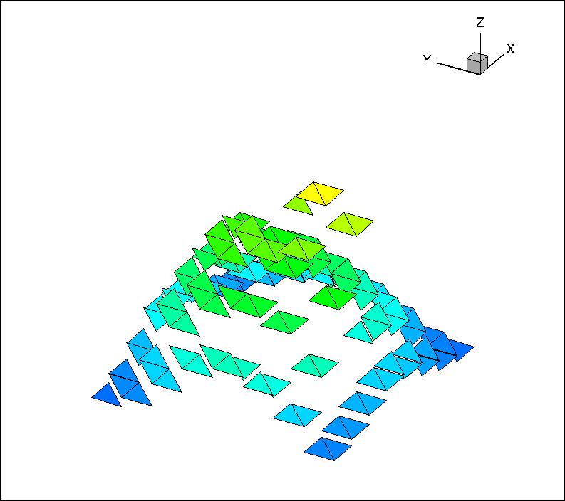
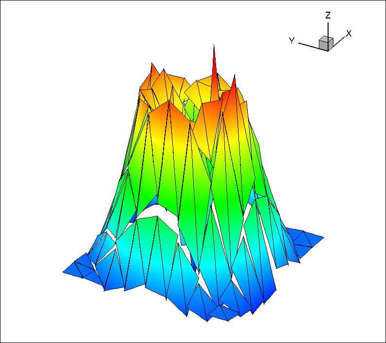
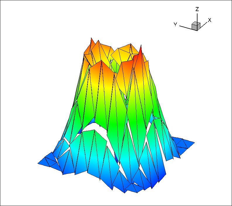
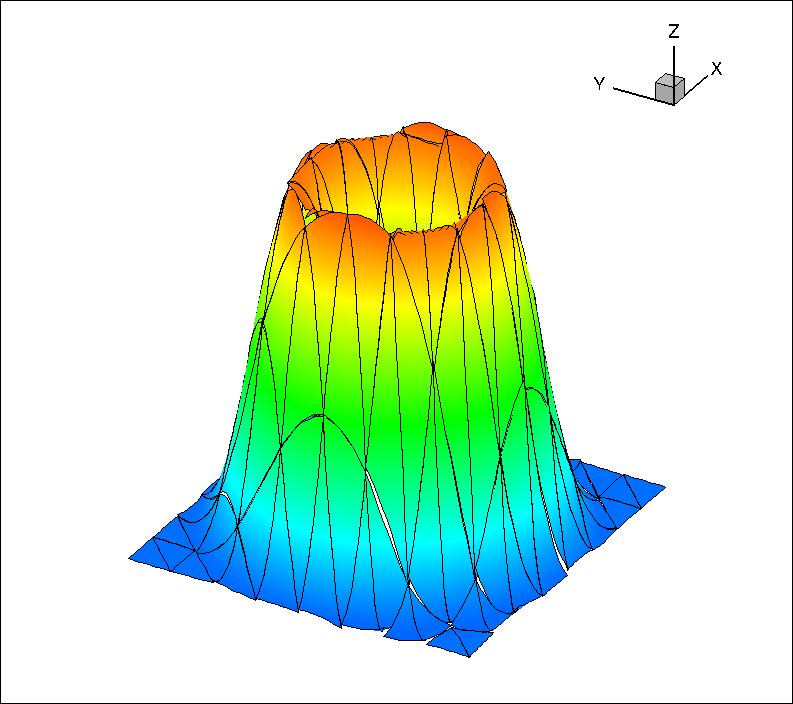
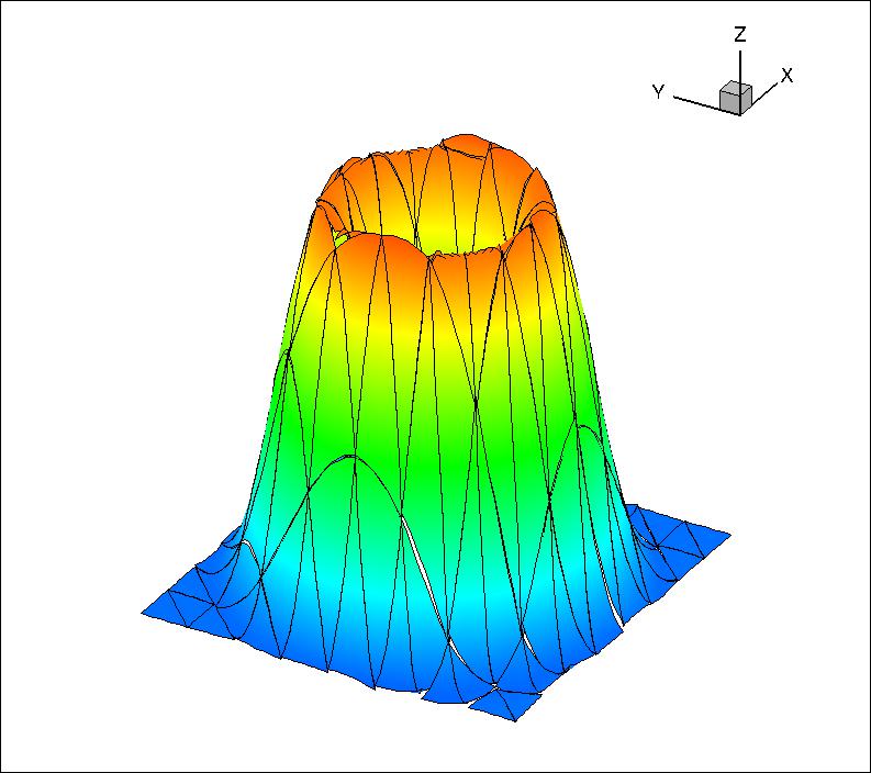
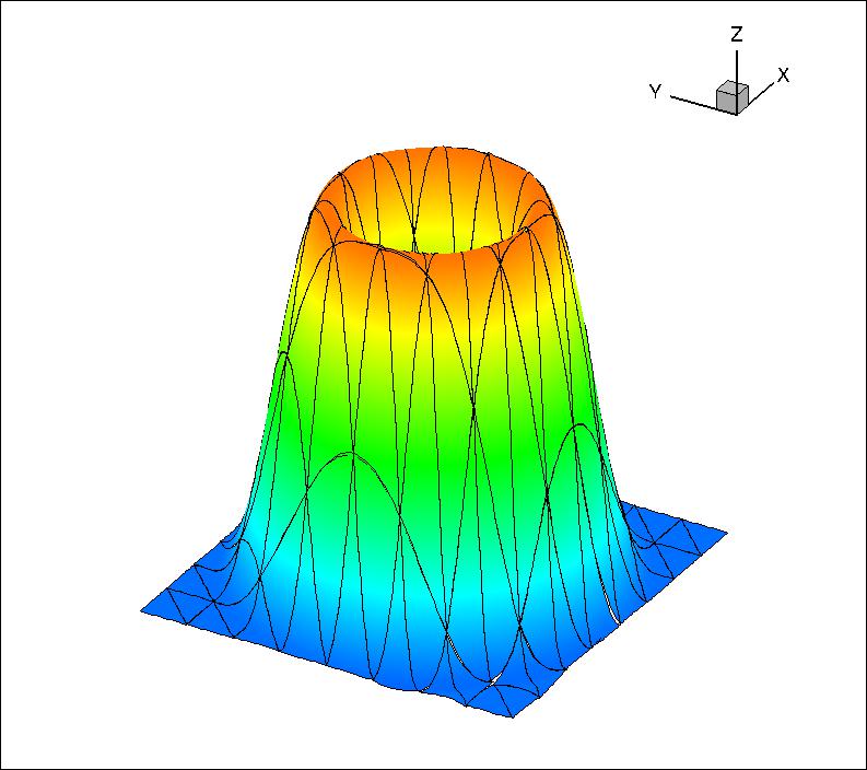
Figure 1. 3D plot of $u_{h}$ for rotating flow test with $\epsilon=10^{-6}$ in 128 elements. Left–Right: $HDG1$, $HDG2$, $HDG3$. Top–Bottom: $P_{0}$–$P_{3}$.

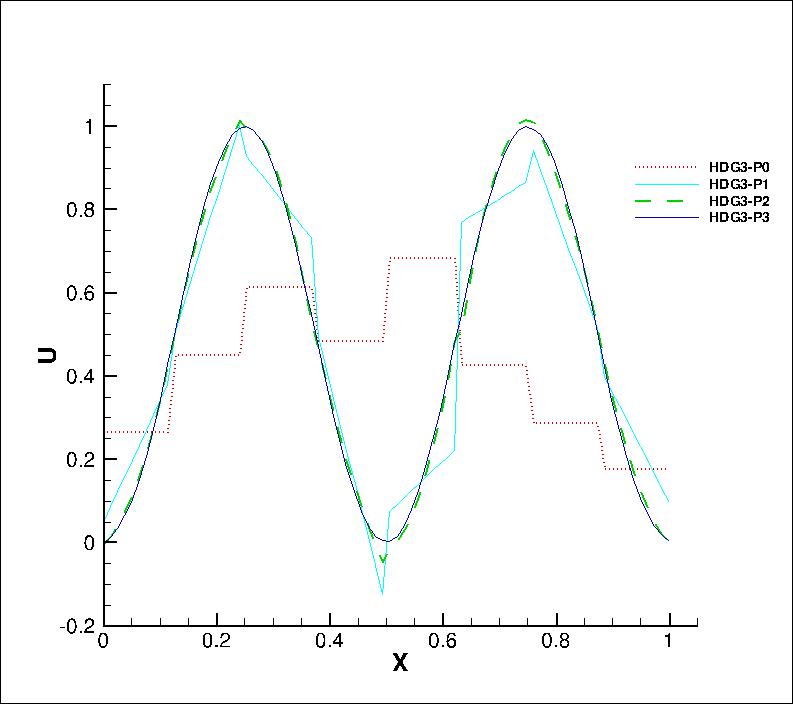
Figure 2. $u_{h}$ along $y=1/2$ for $P_{k}$-$HDG3$ with 128 elements.

Figure 3. A comparison of $P_{0}$-$HDG$ and $P_{3}$-$HDG$. Left: $P_{0}$-$HDG1$ with $8192$ elements; Right $P_{3}$-$HDG1$ with $128$ elements. Top: 3D plot; Bottom: 2D contour.

5.3. An interior layer test

We take $\boldsymbol{\beta}=[1/2,\sqrt{3}/2]^{T}$, $f=0$, and the Dirichlet boundary condition as follows:

$$u=\left\{\begin{tabular}[]{l l}$1$&{ on }$\{y=0,0\leq x\leq 1\}$,\\ $1$&{ on }$\{x=0,0\leq y\leq 1/5\}$,\\ $0$&{ elsewhere.}\end{tabular}\right.$$

It is clear that for $\epsilon$ small, the exact solution produces an interior layer along $\boldsymbol{\beta}$ direction starting from $(0,1/5)$, and boundary layers on the right and top right boundary.

In Fig. 4 and Fig. 5, we plot the computational results in a structured triangular grid of 128 elements for $\epsilon=10^{-3}$ and $\epsilon=10^{-9}$ respectively. In order to better see the performance of the HDG method in capturing interior layers, in Fig. 6, we plot the contour of $u_{h}$ using $P_{k}$-$HDG1$ with $0\leq k\leq 3$ for $\epsilon=10^{-3}$ in three consecutive meshes with the coarsest one consists of 200 elements. Again, all the HDG methods produce quite similar results. Note that, as expected, the piecewise-constant approximations are free of oscillations but extensively smear out the interior layer, while, on the other hand, higher order approximations capture the interior layer within a few elements but produce oscillations within the layer.

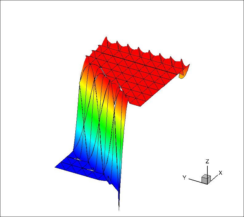
Figure 4. 3D plot of $u_{h}$ for the interior layer test with $\epsilon=10^{-3}$ in 128 elements. Left–Right: $HDG1$, $HDG2$, $HDG3$. Top–Bottom: $P_{0}$–$P_{3}$.

Figure 5. 3D plot of $u_{h}$ for the interior layer test with $\epsilon=10^{-9}$ in 128 elements. Left–Right: $HDG1$, $HDG2$, $HDG3$. Top–Bottom: $P_{0}$–$P_{3}$.

Figure 6. Contour plot of $u_{h}$ using $HDG1$ for the interior layer test with $\epsilon=10^{-3}$. Left to right: three consecutive meshes with the left one consists of a uniform triangulation of 200 elements. Top–Bottom: $P_{0}$–$P_{3}$.

5.4. A boundary layer test

Finally, we take $\boldsymbol{\beta}=[1,1]^{T}$, and choose the source term $f$ so that the exact solution

$$u(x,y)=\sin\frac{\pi\,x}{2}+\sin\frac{\pi\,y}{2}\left(1-\sin\frac{\pi\,x}{2}\right)+\frac{e^{-1/\epsilon}-e^{-(1-x)(1-y)/\epsilon}}{1-e^{-1/\epsilon}}.$$

The solution develops boundary layers along the top and right boundaries for small $\epsilon$ (see Fig. 7 for $\epsilon=10^{-2}$ and Fig. 8 for $\epsilon=10^{-6}$). We take an exact solution which is a slight modification of that considered in [1] so that, away from the boundary layers, our exact solution behaves not like a quadratic polynomial as in [1]. This modification is useful for us to clearly see the orders of convergence for $k=2,3$.

In Fig. 7 and Fig. 8, we plot the exact solution and computational results for $\epsilon=10^{-2}$ and $\epsilon=10^{-6}$ in a structured 200 elements. We find that all the HDG methods produce similar results. The boundary layers are not resolved since the mesh is too coarse.

In Table 4, we show the convergence of $u_{h}$ in $L^{2}$–norm for $\epsilon=10^{-2},10^{-6}$ in the reduced domain $\widetilde{\Omega}=[0,0.9]\times[0,0.9]\subset\Omega$ to exclude the unresolved boundary layers. Just as in the smooth case, the three HDG methods produce very similar convergence results. Hence we only show the computed results for $P_{k}$-$HDG1$ in Table 4. We observe optimal $L^{2}$–convergence rates for $u_{h}$.

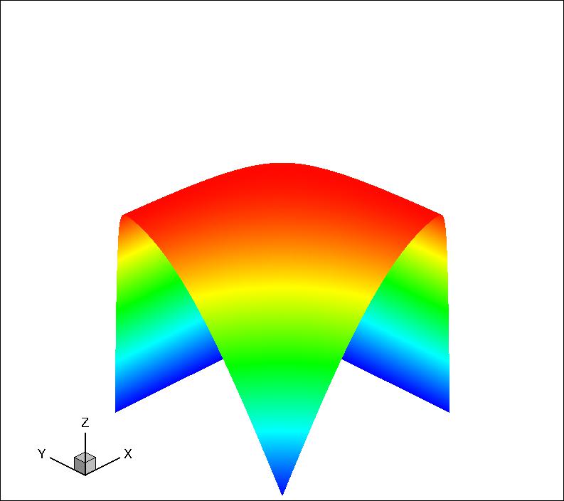
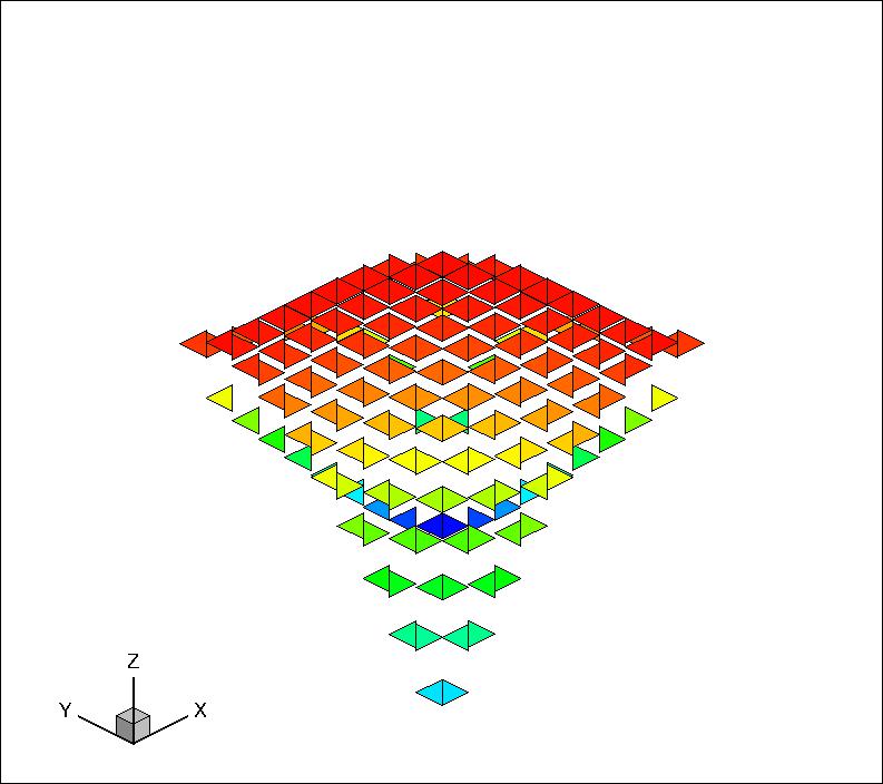
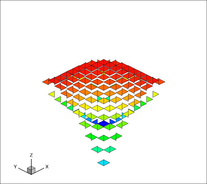
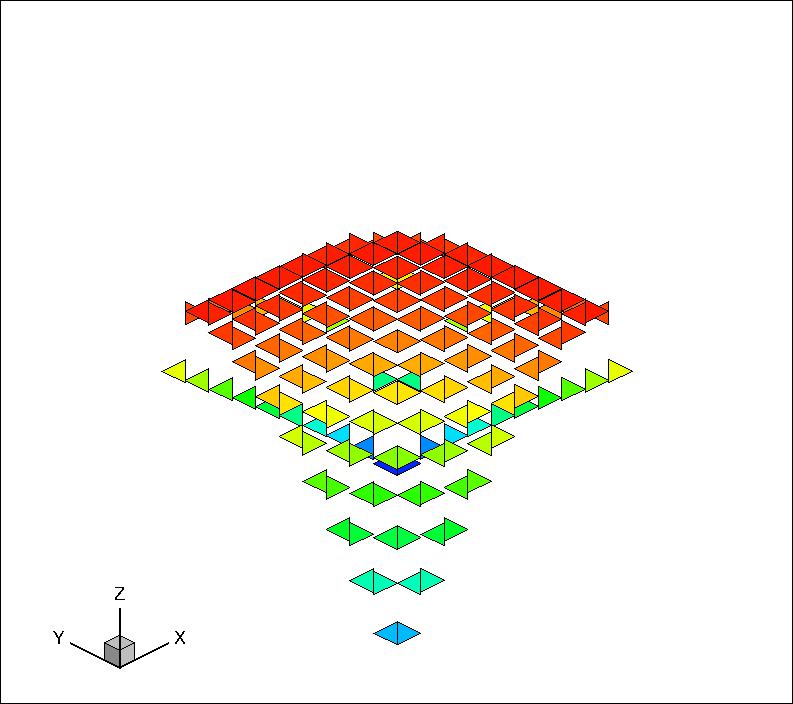
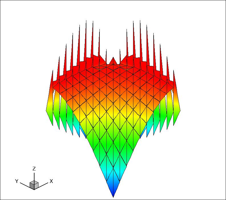
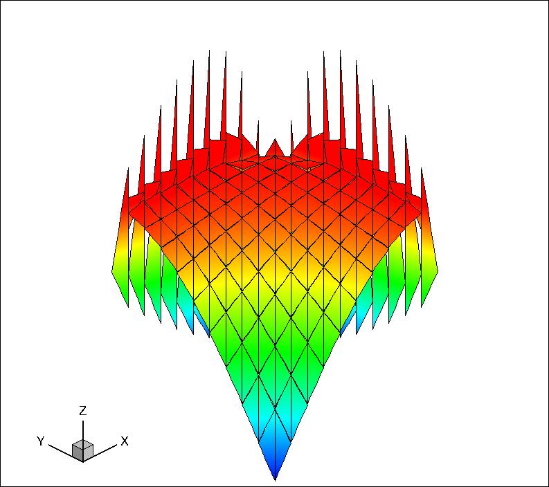
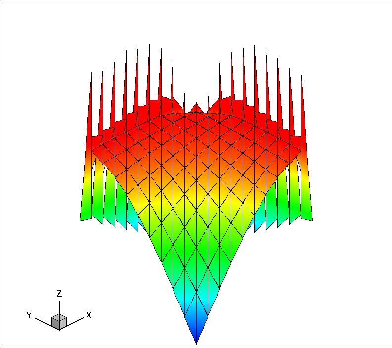
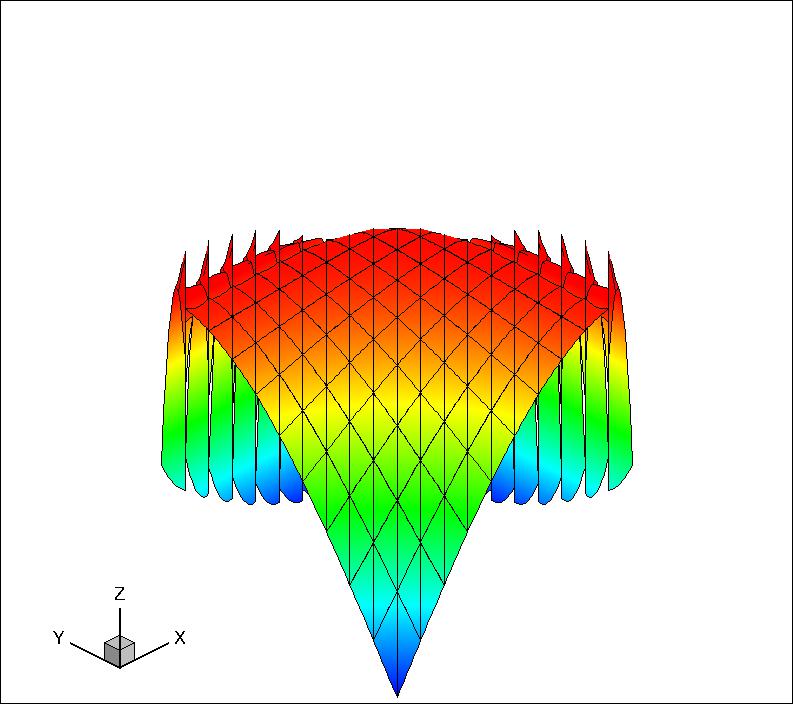
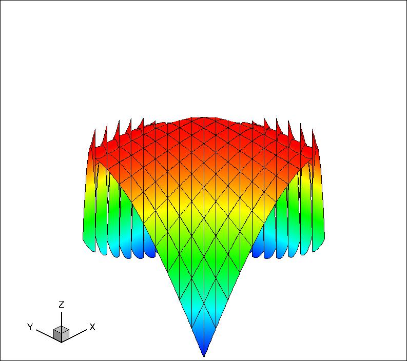
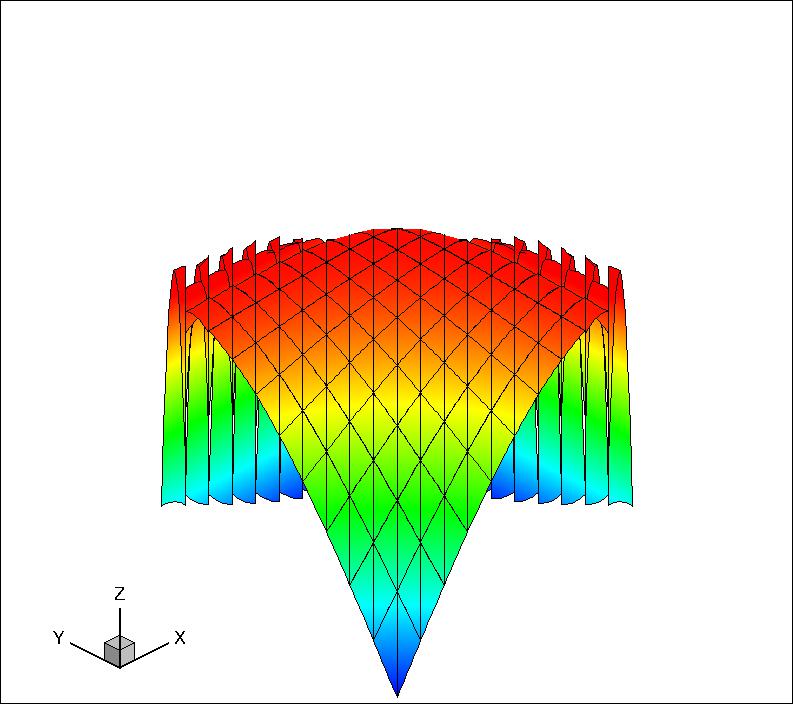
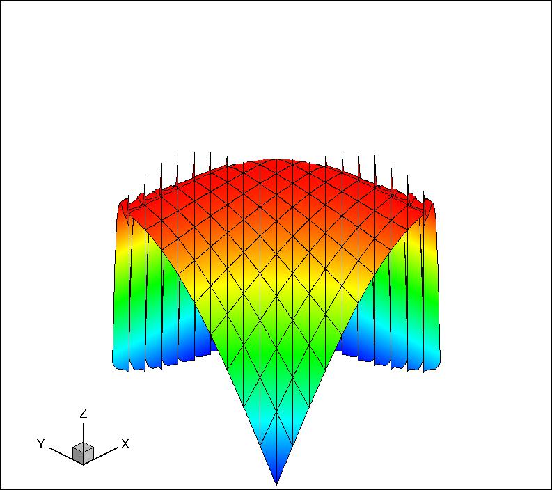
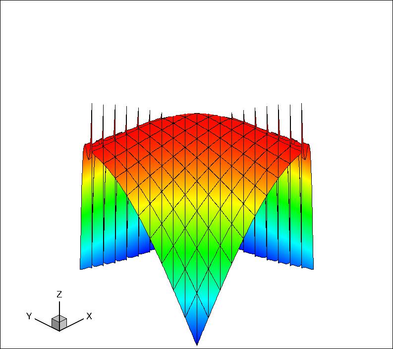
Figure 7. 3D plot of the exact solution and $u_{h}$ for the boundary layer test with $\epsilon=10^{-2}$ in 128 elements. Top center: the exact solution. Left–Right: $HDG1$, $HDG2$, $HDG3$. Top–Bottom: $P_{0}$–$P_{3}$.

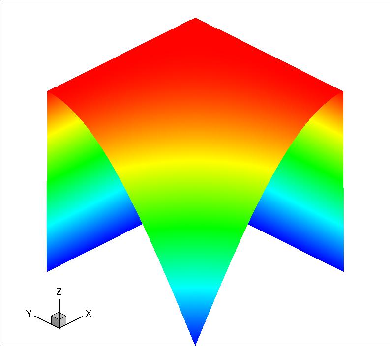
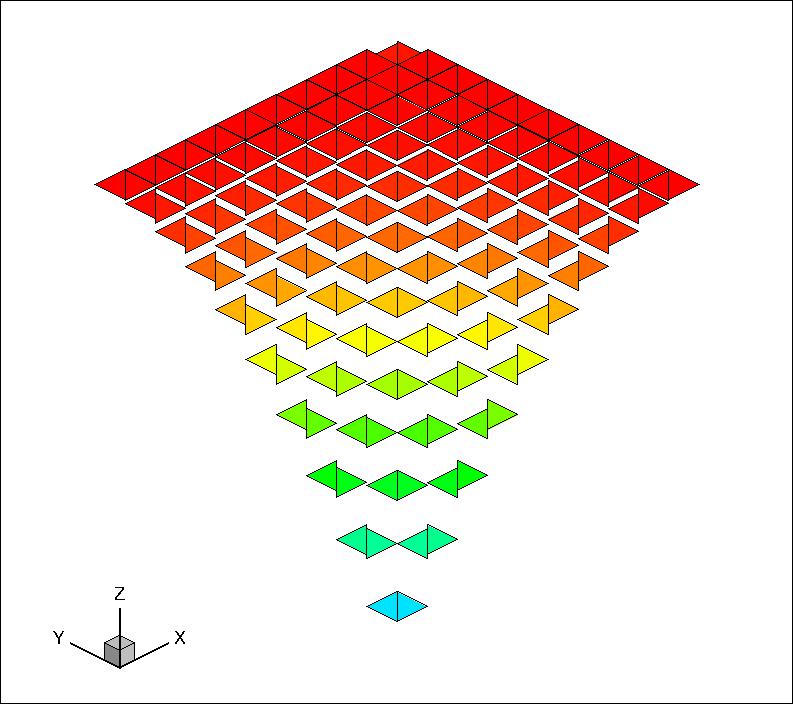
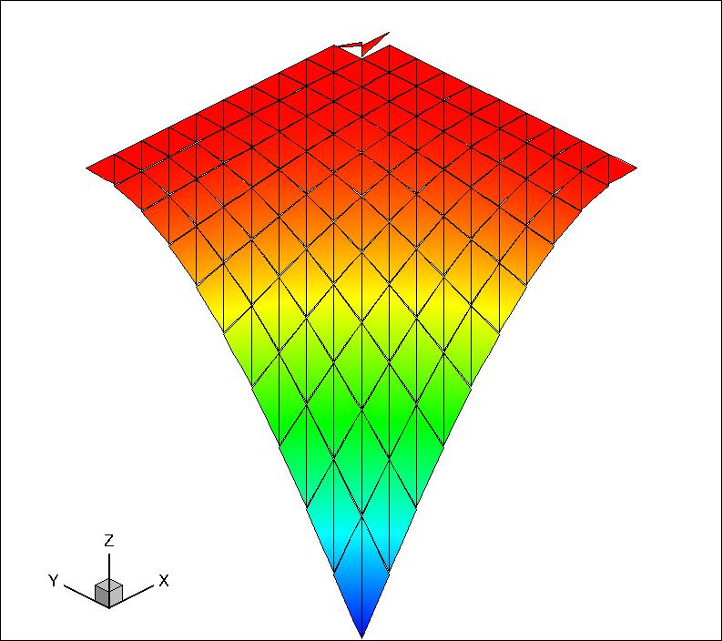
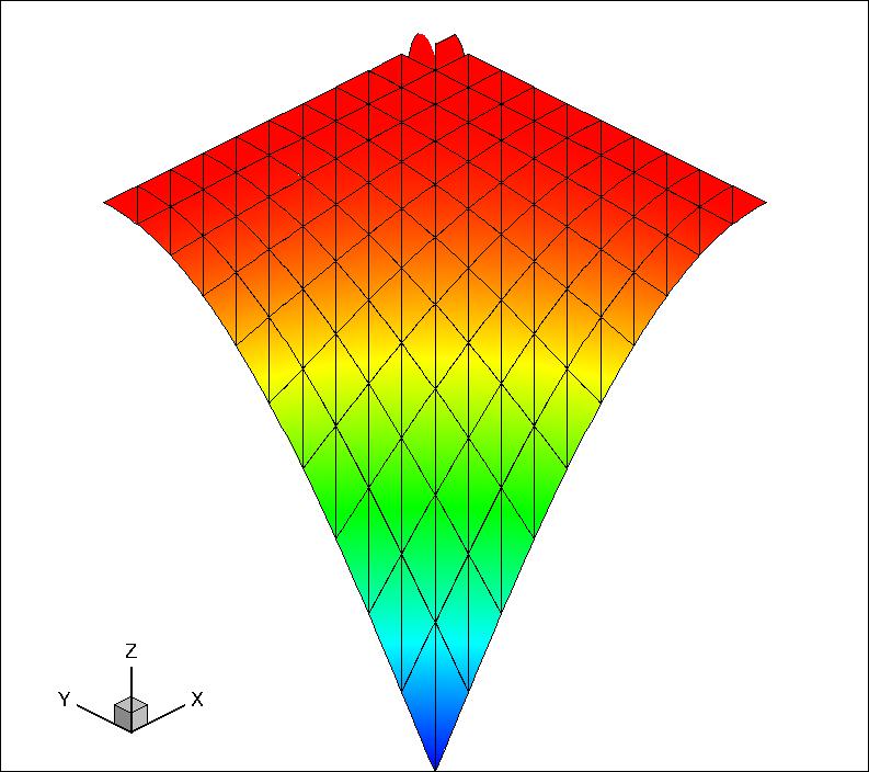
Figure 8. 3D plot of the exact solution and $u_{h}$ for the boundary layer test with $\epsilon=10^{-6}$ in 128 elements. Top center: the exact solution. Left–Right: $HDG1$, $HDG2$, $HDG3$. Top–Bottom: $P_{0}$–$P_{3}$.

$\begin{array}[]{|c|c||c c||c c|}\hline\cr\phantom{\big{|}}\mbox{degree}&\mbox{mesh}&\vrule\lx@intercol\hfil\epsilon=10^{-2}\phantom{\big{|}}\hfil\lx@intercol\vrule\lx@intercol\vrule\lx@intercol&\vrule\lx@intercol\hfil\epsilon=10^{-6}\phantom{\big{|}}\hfil\lx@intercol\vrule\lx@intercol\\ \cline{3-6}\cr\phantom{\big{|}}k&h^{-1}&\mbox{error}&\mbox{order}&\mbox{error}&\mbox{order}\\ \hline\cr&10&3.61\mbox{e-}2&--&3.32\mbox{e-}2&--\\ &20&1.81\mbox{e-}2&0.99&1.67\mbox{e-}2&1.00\\ 0&40&9.06\mbox{e-}3&1.00&8.34\mbox{e-}3&1.00\\ &80&4.52\mbox{e-}3&1.00&4.17\mbox{e-}3&1.00\\ \hline\cr&10&4.22\mbox{e-}3&--&1.20\mbox{e-}3&--\\ &20&8.54\mbox{e-}4&2.30&3.00\mbox{e-}4&2.00\\ 1&40&2.13\mbox{e-}4&2.00&7.51\mbox{e-}5&2.00\\ &80&5.30\mbox{e-}5&2.01&1.88\mbox{e-}5&2.00\\ \hline\cr&10&1.48\mbox{e-}3&--&1.90\mbox{e-}5&--\\ &20&6.66\mbox{e-}5&4.47&2.37\mbox{e-}6&3.00\\ 2&40&8.19\mbox{e-}6&3.02&2.96\mbox{e-}7&3.00\\ &80&1.03\mbox{e-}6&3.00&3.70\mbox{e-}8&3.00\\ \hline\cr&10&4.10\mbox{e-}4&--&3.17\mbox{e-}7&--\\ &20&5.35\mbox{e-}6&6.26&1.99\mbox{e-}8&3.99\\ 3&40&3.56\mbox{e-}7&3.91&1.25\mbox{e-}9&4.00\\ &80&2.27\mbox{e-}8&3.97&7.79\mbox{e-}11&4.00\\ \hline\cr\end{array}$

 

Table 4. History of convergence of $HDG1$ for $\|u-u_{h}\|_{L^{2}(\widetilde{\Omega})}$ when $\epsilon=10^{-2}$ and $\epsilon=10^{-6}$.

5.5. The condition number

Now, we present the condition number of the matrix generated by the original bilinear form $a_{h}$ in (3.2) and the scaled bilinear form $\widetilde{a}_{h}$ in (3.5). We use the same setup as that of the smooth test with two choices of $\boldsymbol{\beta}$. The first choice of $\boldsymbol{\beta}$ is $\boldsymbol{\beta}=[1,2]^{T}$. For this choice, assumption (3.3) is satisfied by both example of $\tau$ in (2.10) and (2.11). Since the condition numbers of all three HDG methods are very similar in our tests, we only present that for $P_{k}$-$HDG1$ in Table 5. Notice that $\mathcal{O}(h^{-2})$ is observed for $\epsilon=1,10^{-3},10^{-9}$ for different polynomial degrees, and that the condition number of the scaled system is similar to that of unscaled system. The second choice of $\boldsymbol{\beta}$ is $\boldsymbol{\beta}=[1,1]^{T}$. For this choice, assumption (3.3) is satisfied by the second choice of $\tau$ in (2.11), but not for the choice (2.10) since the mesh is aligned with $\boldsymbol{\beta}$. However, one can easily modify $\tau$ in $P_{k}$-$HDG1$ and $P_{k}$-$HDG3$ on the aligned faces so that (3.3) holds. We only present the condition numbers for $P_{k}$-$HDG2$ in Table 6. The dependence of the condition number on $\epsilon$ seems to be of order $\mathcal{O}({\epsilon^{-1}})$ for the original system, and we observe a huge improvement of the condition number after scaling for $\epsilon=10^{-9}$. Also, we find that the condition number for the scaled system is of order $\mathcal{O}(h^{-2})$ for $\epsilon=1$, and of order $\mathcal{O}(h^{-1})$ for $\epsilon=10^{-3},10^{-9}$, which is not predicted by our theory.

$\begin{array}[]{|c|c||c|c|c|c|| c|c|c|c|}\hline\cr\phantom{\big{|}}\mbox{$\epsilon$}&\mbox{mesh}&\vrule\lx@intercol\hfil\text{Condition numbers for $a_{h}(\cdot,\cdot)$}\phantom{\big{|}}\hfil\lx@intercol\vrule\lx@intercol\vrule\lx@intercol&\vrule\lx@intercol\hfil\text{Condition numbers for $\widetilde{a}_{h}(\cdot,\cdot)$}\phantom{\big{|}}\hfil\lx@intercol\vrule\lx@intercol\\ \cline{3-10}\cr\phantom{\big{|}}&h^{-1}&\mbox{k=}0&\mbox{k=}1&\mbox{k=}2&\mbox{k=}3&\mbox{k=}0&\mbox{k=}1&\mbox{k=}2&\mbox{k=}3\\ \hline\cr&5&1.11\mbox{e+}2&1.42\mbox{e+}2&2.82\mbox{e+}2&3.31\mbox{e+}2&2.49\mbox{e+}2&2.65\mbox{e+}2&5.30\mbox{e+}2&6.29\mbox{e+}2\\ &10&3.37\mbox{e+}2&5.28\mbox{e+}2&1.06\mbox{e+}3&1.24\mbox{e+}2&6.29\mbox{e+}2&9.83\mbox{e+}2&1.98\mbox{e+}3&2.34\mbox{e+}2\\ 1\mbox{e-}0&20&1.37\mbox{e+}3&2.09\mbox{e+}3&4.17\mbox{e+}3&4.89\mbox{e+}2&2.55\mbox{e+}3&3.89\mbox{e+}3&7.78\mbox{e+}3&9.21\mbox{e+}2\\ &40&5.50\mbox{e+}3&8.32\mbox{e+}3&1.66\mbox{e+}4&1.95\mbox{e+}2&1.03\mbox{e+}4&1.55\mbox{e+}4&3.10\mbox{e+}4&3.67\mbox{e+}2\\ \hline\cr&5&4.86\mbox{e+}1&1.60\mbox{e+}2&3.64\mbox{e+}2&5.00\mbox{e+}2&3.71\mbox{e+}1&1.12\mbox{e+}2&2.44\mbox{e+}2&3.40\mbox{e+}2\\ &10&1.74\mbox{e+}2&5.23\mbox{e+}2&8.79\mbox{e+}2&1.27\mbox{e+}3&1.36\mbox{e+}2&3.75\mbox{e+}2&6.51\mbox{e+}2&8.48\mbox{e+}2\\ 1\mbox{e-}3&20&6.48\mbox{e+}2&1.82\mbox{e+}3&2.35\mbox{e+}3&4.06\mbox{e+}3&5.06\mbox{e+}2&1.25\mbox{e+}3&1.17\mbox{e+}3&2.50\mbox{e+}3\\ &40&2.48\mbox{e+}3&6.94\mbox{e+}3&8.76\mbox{e+}3&1.49\mbox{e+}4&1.94\mbox{e+}3&4.44\mbox{e+}3&5.98\mbox{e+}3&8.96\mbox{e+}3\\ \hline\cr&5&4.90\mbox{e+}1&1.69\mbox{e+}2&4.21\mbox{e+}2&5.76\mbox{e+}2&3.73\mbox{e+}1&9.57\mbox{e+}1&2.97\mbox{e+}2&3.80\mbox{e+}2\\ &10&1.74\mbox{e+}2&5.38\mbox{e+}2&1.17\mbox{e+}3&1.52\mbox{e+}3&1.36\mbox{e+}2&4.04\mbox{e+}2&9.11\mbox{e+}2&1.05\mbox{e+}3\\ 1\mbox{e-}9&20&6.49\mbox{e+}2&1.94\mbox{e+}3&3.76\mbox{e+}3&4.73\mbox{e+}3&5.05\mbox{e+}2&1.46\mbox{e+}3&2.94\mbox{e+}3&3.40\mbox{e+}3\\ &40&2.50\mbox{e+}3&7.06\mbox{e+}3&1.34\mbox{e+}4&1.65\mbox{e+}4&1.93\mbox{e+}3&5.37\mbox{e+}3&9.45\mbox{e+}3&1.25\mbox{e+}4\\ \hline\cr\end{array}$

 

Table 5. Condition numbers for $HDG1$ when $\boldsymbol{\beta}=[1,2]^{T}$.

$\begin{array}[]{|c|c||c|c|c|c|| c|c|c|c|}\hline\cr\phantom{\big{|}}\mbox{$\epsilon$}&\mbox{mesh}&\vrule\lx@intercol\hfil\text{Condition numbers for $a_{h}(\cdot,\cdot)$}\phantom{\big{|}}\hfil\lx@intercol\vrule\lx@intercol\vrule\lx@intercol&\vrule\lx@intercol\hfil\text{Condition numbers for $\widetilde{a}_{h}(\cdot,\cdot)$}\phantom{\big{|}}\hfil\lx@intercol\vrule\lx@intercol\\ \cline{3-10}\cr\phantom{\big{|}}&h^{-1}&\mbox{k=}0&\mbox{k=}1&\mbox{k=}2&\mbox{k=}3&\mbox{k=}0&\mbox{k=}1&\mbox{k=}2&\mbox{k=}3\\ \hline\cr&5&9.99\mbox{e+}1&1.41\mbox{e+}2&2.82\mbox{e+}2&3.31\mbox{e+}2&1.16\mbox{e+}2&1.96\mbox{e+}2&3.92\mbox{e+}2&4.64\mbox{e+}2\\ &10&3.40\mbox{e+}2&5.34\mbox{e+}2&1.07\mbox{e+}3&1.25\mbox{e+}2&4.35\mbox{e+}2&6.82\mbox{e+}2&1.37\mbox{e+}3&1.61\mbox{e+}2\\ 1\mbox{e-}0&20&1.38\mbox{e+}3&2.12\mbox{e+}3&4.23\mbox{e+}3&4.96\mbox{e+}2&1.77\mbox{e+}3&2.71\mbox{e+}3&5.41\mbox{e+}3&6.38\mbox{e+}2\\ &40&5.57\mbox{e+}3&8.44\mbox{e+}3&1.68\mbox{e+}4&1.98\mbox{e+}2&7.12\mbox{e+}3&1.08\mbox{e+}4&2.15\mbox{e+}4&2.54\mbox{e+}2\\ \hline\cr&5&2.01\mbox{e+}2&6.63\mbox{e+}2&9.06\mbox{e+}2&1.55\mbox{e+}3&2.48\mbox{e+}2&1.81\mbox{e+}3&7.02\mbox{e+}3&9.83\mbox{e+}3\\ &10&4.00\mbox{e+}2&1.41\mbox{e+}3&1.62\mbox{e+}3&3.27\mbox{e+}3&5.63\mbox{e+}2&2.34\mbox{e+}3&7.45\mbox{e+}3&1.16\mbox{e+}4\\ 1\mbox{e-}3&20&1.25\mbox{e+}3&4.42\mbox{e+}3&4.98\mbox{e+}3&9.57\mbox{e+}3&1.20\mbox{e+}3&3.99\mbox{e+}3&9.01\mbox{e+}3&1.66\mbox{e+}4\\ &40&4.69\mbox{e+}3&1.63\mbox{e+}4&1.86\mbox{e+}4&3.12\mbox{e+}4&2.60\mbox{e+}3&7.29\mbox{e+}3&1.32\mbox{e+}4&2.49\mbox{e+}4\\ \hline\cr&5&1.43\mbox{e+}8&4.02\mbox{e+}8&6.04\mbox{e+}8&7.34\mbox{e+}8&2.38\mbox{e+}2&2.07\mbox{e+}3&1.23\mbox{e+}4&2.49\mbox{e+}4\\ &10&1.31\mbox{e+}8&3.84\mbox{e+}8&5.68\mbox{e+}8&7.03\mbox{e+}8&5.35\mbox{e+}2&4.66\mbox{e+}3&2.77\mbox{e+}4&5.60\mbox{e+}4\\ 1\mbox{e-}9&20&1.25\mbox{e+}8&3.75\mbox{e+}8&5.51\mbox{e+}8&6.87\mbox{e+}8&1.13\mbox{e+}3&9.84\mbox{e+}3&5.85\mbox{e+}4&1.12\mbox{e+}5\\ &40&1.22\mbox{e+}8&3.70\mbox{e+}8&5.42\mbox{e+}8&6.79\mbox{e+}8&2.32\mbox{e+}3&2.02\mbox{e+}4&1.20\mbox{e+}5&2.30\mbox{e+}5\\ \hline\cr\end{array}$

 

Table 6. Condition numbers for $HDG2$ when $\boldsymbol{\beta}=[1,1]^{T}$.

Acknowledgements. The authors would like to thank Professor Bernardo Cockburn for constructive criticism leading to a better presentation of the material in this paper. The authors would also like to thank one of the referees for pointing out the paper by Egger and Schöberl [26] and for suggesting to comment on the relation of the HDG method to the MH–DG method in [26], as was done in Appendix A. The work of Weifeng Qiu was supported by City University of Hong Kong under start-up grant (No. 7200324).

Appendix A The relation between the HDG method and the MH–DG method in [26]

In this section, we establish the relation between the HDG method (2.4) and the MH–DG considered in [26]. We first present the MH–DG method for equations (1.1) under the condition that $g=0$ and $\boldsymbol{\beta}\in H(\mathrm{div};\Omega)$ is constant in each element. Then, we show that this method coincides with the HDG method (2.4) when using the same approximation spaces and choosing the stability function $\tau$ to be (2.10).

The MH–DG method seeks an approximation $(\boldsymbol{q}_{h},u_{h},\lambda_{h})\in\widetilde{\boldsymbol{V}}_{h}\times W_{h}\times M_{h}(0)$ so that

$$B_{h}((\boldsymbol{q}_{h},u_{h},\lambda_{h}),(\boldsymbol{r},w,\mu))=(f,w)_{{\mathcal{T}_{h}}},$$ (A.1)

for all $(\boldsymbol{r},w,\mu)\in\widetilde{\boldsymbol{V}}_{h}\times W_{h}\times M_{h}(0)$, where $W_{h}$ and $M_{h}(0)$ is defined in (2.3) and $\widetilde{\boldsymbol{V}}_{h}$ is the so called Raviart–Thomas space, slightly larger than $\boldsymbol{V}_{h}$, defined as follows

$$\widetilde{\boldsymbol{V}}_{h} =\{\boldsymbol{r}\in L^{2}(\Omega;\mathbb{R}^{d}):\boldsymbol{r}|_{K}\in P_{k}(K;\mathbb{R}^{d})+\boldsymbol{x}P_{k}(K)\quad\forall K\in\mathcal{T}_{h}\},$$

and

$$B_{h}((\boldsymbol{q},u,\lambda),(\boldsymbol{r},w,\mu))= \;(\epsilon^{-1}\boldsymbol{q},\boldsymbol{r})_{\mathcal{T}_{h}}-(u,\nabla\cdot\boldsymbol{r})_{\mathcal{T}_{h}}+\langle\lambda,\boldsymbol{r}\cdot\boldsymbol{n}\rangle_{\partial\mathcal{T}_{h}}$$

$$-(\boldsymbol{q}+\boldsymbol{\beta}u,\nabla w)_{\mathcal{T}_{h}}+\langle\boldsymbol{q}\cdot\boldsymbol{n}+\boldsymbol{\beta}\cdot\boldsymbol{n}\{\lambda/u\},w-\mu\rangle_{\partial\mathcal{T}_{h}},$$

where

$$\{\lambda/u\}:=\left\{\begin{tabular}[]{c c}$\lambda$,&\quad\text{ if } $\boldsymbol{\beta}\cdot\boldsymbol{n}<0$,\\ $u$,&\quad\text{ if } $\boldsymbol{\beta}\cdot\boldsymbol{n}\geq 0$.\\ \end{tabular}\right.$$

Comparing the bilinear form for the HDG method (4.1) with approximation spaces $\widetilde{\boldsymbol{V}}_{h}\times W_{h}\times M_{h}(0)$ and the stability function $\tau$ in (2.10) and that for the MH–DG method in (A.1), we notice that the only difference lies in the definition of the numerical flux $(\widehat{\boldsymbol{q}}_{h}+\widehat{\boldsymbol{\beta}u_{h}})\cdot\boldsymbol{n}$ and $\boldsymbol{q}_{h}\cdot\boldsymbol{n}+\boldsymbol{\beta}\cdot\boldsymbol{n}\{\lambda/u\}$. However, by the following simple calculation, we observe that the two numerical flux are actually the same:

$$(\widehat{\boldsymbol{q}}_{h}+\widehat{\boldsymbol{\beta}u_{h}})\cdot\boldsymbol{n} =\;{\boldsymbol{q}}_{h}\cdot\boldsymbol{n}+{\boldsymbol{\beta}\cdot\boldsymbol{n}\lambda_{h}}+\tau(u_{h}-\lambda_{h})$$

$$=\;{\boldsymbol{q}}_{h}\cdot\boldsymbol{n}+{\boldsymbol{\beta}\cdot\boldsymbol{n}\lambda_{h}}+\max(\boldsymbol{\beta}\cdot\boldsymbol{n},0)(u_{h}-\lambda_{h})$$

$$=\;\left\{\begin{tabular}[]{c c}$\boldsymbol{q}_{h}\cdot\boldsymbol{n}+\boldsymbol{\beta}\cdot\boldsymbol{n}\lambda_{h}$,&\quad\text{ if } $\boldsymbol{\beta}\cdot\boldsymbol{n}<0$\\ $\boldsymbol{q}_{h}\cdot\boldsymbol{n}+\boldsymbol{\beta}\cdot\boldsymbol{n}u_{h}$,&\quad\text{ if } $\boldsymbol{\beta}\cdot\boldsymbol{n}\geq 0$\end{tabular}\right.$$

$$=\;\boldsymbol{q}_{h}\cdot\boldsymbol{n}+\boldsymbol{\beta}\cdot\boldsymbol{n}\{\lambda_{h}/u_{h}\}.$$

Hence, these two methods coincide.

Appendix B Conditioning of the HDG methods

In this section, we give a proof of Theorem 3.2. Again, the key idea is to recover an estimate of the $L^{2}$–norm of $u_{h}$, see the estimate (B.5) below. By similar argument in the proof of Lemma 4.4, we have the following local energy estimate:

Lemma B.1.

If $\epsilon\leq\mathcal{O}(h)$, then there is $h_{0}>0$, which is independent of $\epsilon$ and $h$, such that for any $\lambda\in M_{h}(0)$ and $K\in\mathcal{T}_{h}$,

$$\epsilon^{-1/2}\|\boldsymbol{q}_{h}^{\lambda}\|_{K}+\|u_{h}^{\lambda}\|_{K}+\||\tau-\frac{1}{2}\boldsymbol{\beta}\cdot\boldsymbol{n}|^{1/2}u_{h}^{\lambda}\|_{\partial K}\leq C\||\tau-\frac{1}{2}\boldsymbol{\beta}\cdot\boldsymbol{n}|^{1/2}\lambda\|_{\partial K},$$ (B.1)

if $h<h_{0}$.

For all $(\boldsymbol{\sigma},v,\lambda),(\boldsymbol{r},w,\mu)\in H^{1}(\mathcal{T}_{h};\mathbb{R}^{d})\times H^{1}(\mathcal{T}_{h})\times L^{2}(\mathcal{E}_{h})$, we define

$$b_{h}((\boldsymbol{\sigma},v,\lambda),(\boldsymbol{r},w,\mu))= \;(\epsilon^{-1}\boldsymbol{\sigma},\boldsymbol{r})_{\mathcal{T}_{h}}+\langle\tau(v-\lambda),w-\mu\rangle_{\partial\mathcal{T}_{h}}$$

$$-(\boldsymbol{\beta}v,\nabla w)_{\mathcal{T}_{h}}+\langle(\boldsymbol{\beta}\cdot\boldsymbol{n})\lambda,w-\mu\rangle_{\partial\mathcal{T}_{h}}-((\nabla\cdot\boldsymbol{\beta})v,w)_{\mathcal{T}_{h}},$$

The next result is similar to Lemma 4.4.

Lemma B.2.

If $\epsilon\leq\mathcal{O}(h)$, then there is $h_{0}>0$, which is independent of $\epsilon$ and $h$, such that for any $\lambda\in M_{h}(0)$,

$$\epsilon^{-1}\|\boldsymbol{q}_{h}^{\lambda}\|_{\mathcal{T}_{h}}^{2}+\|u_{h}^{\lambda}\|_{\mathcal{T}_{h}}^{2}+\||\tau-\frac{1}{2}\boldsymbol{\beta}\cdot\boldsymbol{n}|^{1/2}(u_{h}^{\lambda}-\lambda)\|_{\partial\mathcal{T}_{h}}^{2}$$

$$\leq Cb_{h}((\boldsymbol{q}_{h}^{\lambda},u_{h}^{\lambda},\lambda),(\boldsymbol{q}_{h}^{(P_{0,M}\varphi)\lambda},u_{h}^{(P_{0,M}\varphi)\lambda},(P_{0,M}\varphi)\lambda)),$$

if $h<h_{0}$. Here, the weight function $\varphi=e^{-\psi}+\chi$ is introduced in (4.4). $P_{0,M}$ is the $L^{2}$–orthogonal projection onto $P_{0}(\mathcal{E}_{h})$.

Remark B.3.

Notice that in general, the space $\{(\boldsymbol{q}_{h}^{m},u_{h}^{m},m):m\in M_{h}(0)\}$ is a non-trivial subspace of $\boldsymbol{V}_{h}\times W_{h}\times M_{h}(0)$. Then, given $m\in M_{h}$, $(\boldsymbol{\Pi}_{h}(\varphi\boldsymbol{q}_{h}^{m}),P_{h}(\varphi u_{h}^{m}),P_{M}(\varphi m))$ is not necessarily contained in $\{(\boldsymbol{q}_{h}^{m},u_{h}^{m},m):m\in M_{h}\}$. So, the proof of Lemma B.2 can not be derived from the stability of HDG methods in Lemma 4.4.

Proof.

We accomplish the proof in the following steps.

(I) By the same argument in the proof of Lemma 4.1, if $h$ is small enough (independent of $\epsilon$), then

$$\epsilon^{-1}\chi\|\boldsymbol{q}_{h}^{\lambda}\|_{\mathcal{T}_{h}}^{2}+\|u_{h}^{\lambda}\|_{\mathcal{T}_{h}}^{2}+\chi\||\tau-\frac{1}{2}\boldsymbol{\beta}\cdot\boldsymbol{n}|^{1/2}(u_{h}^{\lambda}-\lambda)\|_{\partial\mathcal{T}_{h}}^{2}$$

$$\leq Cb_{h}((\boldsymbol{q}_{h}^{\lambda},u_{h}^{\lambda},\lambda),(\varphi\boldsymbol{q}_{h}^{\lambda},\varphi u_{h}^{\lambda},\varphi\lambda)).$$

(II) By similar argument in the proof of Lemma 4.4, if we choose $\chi$ big enough and $h$ small enough (both are independent of $\epsilon$), then

$$\epsilon^{-1}\chi\|\boldsymbol{q}_{h}^{\lambda}\|_{\mathcal{T}_{h}}^{2}+\|u_{h}^{\lambda}\|_{\mathcal{T}_{h}}^{2}+\chi\||\tau-\frac{1}{2}\boldsymbol{\beta}\cdot\boldsymbol{n}|^{1/2}(\mathcal{U}\lambda-\lambda)\|_{\partial\mathcal{T}_{h}}^{2}$$

$$\leq Cb_{h}((\boldsymbol{q}_{h}^{\lambda},u_{h}^{\lambda},\lambda),((P_{0,h}\varphi)\boldsymbol{q}_{h}^{\lambda},P_{h}(\varphi u_{h}^{\lambda}),(P_{0,M}\varphi)\lambda)).$$

Here, we define $P_{0,h}\varphi$ to be the average of $\varphi$ on every element $K\in\mathcal{T}_{h}$.

(III) Now, we want to bound $b_{h}((\boldsymbol{q}_{h}^{\lambda},u_{h}^{\lambda},\lambda),((P_{0,h}\varphi)\boldsymbol{q}_{h}^{\lambda},(P_{0,h}\varphi)u_{h}^{\lambda},(P_{0,M}\varphi)\lambda))$ from below. Notice that

$$b_{h}((\boldsymbol{q}_{h}^{\lambda},u_{h}^{\lambda},\lambda),((P_{0,h}\varphi)\boldsymbol{q}_{h}^{\lambda},(P_{0,h}\varphi)u_{h}^{\lambda},(P_{0,M}\varphi)\lambda))$$

$$= b_{h}((\boldsymbol{q}_{h}^{\lambda},u_{h}^{\lambda},\lambda),((P_{0,h}\varphi)\boldsymbol{q}_{h}^{\lambda},P_{h}(\varphi u_{h}^{\lambda}),(P_{0,M}\varphi)\lambda))$$

$$+(\boldsymbol{\beta}\cdot\nabla u_{h}^{\lambda},P_{h}(\varphi u_{h}^{\mu})-(P_{0,h}\varphi)u_{h}^{\mu})_{\mathcal{T}_{h}}$$

$$+\langle(\tau-\boldsymbol{\beta}\cdot\boldsymbol{n})(u_{h}^{\lambda}-\lambda),P_{h}(\varphi u_{h}^{\mu})-(P_{0,h}\varphi)u_{h}^{\mu}\rangle_{\partial\mathcal{T}_{h}}.$$

By (3.1b), we have

$$b_{h}((\boldsymbol{q}_{h}^{\lambda},u_{h}^{\lambda},\lambda),((P_{0,h}\varphi)\boldsymbol{q}_{h}^{\lambda},(P_{0,h}\varphi)u_{h}^{\lambda},(P_{0,M}\varphi)\lambda))$$ (B.2)

$$= b_{h}((\boldsymbol{q}_{h}^{\lambda},u_{h}^{\lambda},\lambda),((P_{0,h}\varphi)\boldsymbol{q}_{h}^{\lambda},P_{h}(\varphi u_{h}^{\lambda}),(P_{0,M}\varphi)\lambda))$$

$$-(\nabla\cdot\boldsymbol{q}_{h}^{\lambda},P_{h}(\varphi u_{h}^{\mu})-(P_{0,h}\varphi)u_{h}^{\mu})_{\mathcal{T}_{h}}.$$

By inverse inequality to $\nabla\cdot\boldsymbol{q}_{h}^{\lambda}$ and assumption $\epsilon\leq\mathcal{O}(h)$, we have

$$\|\nabla\cdot\boldsymbol{q}_{h}^{\lambda}\|_{\mathcal{T}_{h}}\leq C\epsilon^{-1/2}h^{-1/2}\|\boldsymbol{q}_{h}^{\lambda}\|_{\mathcal{T}_{h}}.$$

In addition, we have

$$\|P_{h}(\varphi u_{h}^{\mu})-(P_{0,h}\varphi)u_{h}^{\mu}\|_{\mathcal{T}_{h}}\leq Ch\|u_{h}^{\mu}\|_{\mathcal{T}_{h}}.$$

So, if $h$ is small enough (independent of $\epsilon,\chi$), we have

$$\chi\epsilon^{-1}\|\boldsymbol{q}_{h}^{\lambda}\|_{\mathcal{T}_{h}}^{2}+\|u_{h}^{\lambda}\|_{\mathcal{T}_{h}}^{2}+\chi\||\tau-\frac{1}{2}\boldsymbol{\beta}\cdot\boldsymbol{n}|^{1/2}(u_{h}^{\lambda}-\lambda)\|_{\partial\mathcal{T}_{h}}^{2}$$ (B.3)

$$\leq Cb_{h}((\boldsymbol{q}_{h}^{\lambda},u_{h}^{\lambda},\lambda),((P_{0,h}\varphi)\boldsymbol{q}_{h}^{\lambda},(P_{0,h}\varphi)u_{h}^{\lambda},(P_{0,M}\varphi)\lambda)).$$

(IV) Now, we want to bound $b_{h}((\boldsymbol{q}_{h}^{\lambda},u_{h}^{\lambda},\lambda),((P_{0,h}\varphi)\boldsymbol{q}_{h}^{\lambda},u_{h}^{(P_{0,M}\varphi)\lambda},(P_{0,M}\varphi)\lambda))$ from below. Similar to (B.2), we have

$$b_{h}((\boldsymbol{q}_{h}^{\lambda},u_{h}^{\lambda},\lambda),((P_{0,h}\varphi)\boldsymbol{q}_{h}^{\lambda},u_{h}^{(P_{0,M}\varphi)\lambda},(P_{0,M}\varphi)\lambda))$$ (B.4)

$$= b_{h}((\boldsymbol{q}_{h}^{\lambda},u_{h}^{\lambda},\lambda),((P_{0,h}\varphi)\boldsymbol{q}_{h}^{\lambda},(P_{0,h}\varphi)u_{h}^{\lambda},(P_{0,M}\varphi)\lambda))$$

$$-(\nabla\cdot\boldsymbol{q}_{h}^{\lambda},(P_{0,h}\varphi)u_{h}^{\lambda}-u_{h}^{(P_{0,M}\varphi)\lambda})_{\mathcal{T}_{h}}.$$

Since $\lambda\rightarrow u_{h}^{\lambda}$ is linear and (B.1), then for any $K\in\mathcal{T}_{h}$,

$$\|(P_{0,h}\varphi)u_{h}^{\lambda}-u_{h}^{(P_{0,M}\varphi)\lambda}\|_{K}$$

$$= \|u_{h}^{(P_{0,h}\varphi)\lambda}-u_{h}^{(P_{0,M}\varphi)\lambda}\|_{K}$$

$$\leq C\||\tau-\frac{1}{2}\boldsymbol{\beta}\cdot\boldsymbol{n}|^{1/2}((P_{0,h}\varphi)\lambda-(P_{0,M}\varphi)\lambda)\|_{\partial K}$$

$$\leq Ch\||\tau-\frac{1}{2}\boldsymbol{\beta}\cdot\boldsymbol{n}|^{1/2}\lambda\|_{\partial K}$$

$$\leq Ch^{1/2}\left(\|u_{h}^{\lambda}\|_{K}^{2}+\Sigma_{F\in\mathcal{E}(K)}\||\tau-\frac{1}{2}\boldsymbol{\beta}\cdot\boldsymbol{n}|^{1/2}(u_{h}^{\lambda}-\lambda)\|_{F}^{2}\right)^{1/2}.$$

Recall that by an inverse inequality to $\nabla\cdot\boldsymbol{q}_{h}^{\lambda}$ and assumption $\epsilon\leq\mathcal{O}(h)$,

$$\|\nabla\cdot\boldsymbol{q}_{h}^{\lambda}\|_{\mathcal{T}_{h}}\leq C\epsilon^{-1/2}h^{-1/2}\|\boldsymbol{q}_{h}^{\lambda}\|_{\mathcal{T}_{h}}.$$

So, if $\chi$ is big enough (independent of $\epsilon,h$), we have

$$\epsilon^{-1}\|\boldsymbol{q}_{h}^{\lambda}\|_{\mathcal{T}_{h}}^{2}+\|u_{h}^{\lambda}\|_{\mathcal{T}_{h}}^{2}+\||\tau-\frac{1}{2}\boldsymbol{\beta}\cdot\boldsymbol{n}|^{1/2}(u_{h}^{\lambda}-\lambda)\|_{\partial\mathcal{T}_{h}}^{2}$$

$$\leq Cb_{h}((\boldsymbol{q}_{h}^{\lambda},u_{h}^{\lambda},\lambda),((P_{0,h}\varphi)\boldsymbol{q}_{h}^{\lambda},u_{h}^{(P_{0,M}\varphi)\lambda},(P_{0,M}\varphi)\lambda)).$$

(V) By (B.1), (B.3), (3.3) and the fact that $\lambda\rightarrow\boldsymbol{q}_{h}^{\lambda}$ is linear, we have

$$\epsilon^{-1}\|\boldsymbol{q}_{h}^{\lambda}\|_{\mathcal{T}_{h}}^{2}+\|u_{h}^{\lambda}\|_{\mathcal{T}_{h}}^{2}+\||\tau-\frac{1}{2}\boldsymbol{\beta}\cdot\boldsymbol{n}|^{1/2}(u_{h}^{\lambda}-\lambda)\|_{\partial\mathcal{T}_{h}}^{2}$$

$$\leq Cb_{h}((\boldsymbol{q}_{h}^{\lambda},u_{h}^{\lambda},\lambda),(\boldsymbol{q}_{h}^{(P_{0,M}\varphi)\lambda},u_{h}^{(P_{0,M}\varphi)\lambda},(P_{0,M}\varphi)\lambda))$$

if $h$ is small enough (independent of $\epsilon$).

So, we can conclude the proof is complete. ∎

Now, we are ready to prove Theorem 3.2. By the definition of $\tilde{a}_{h}$ in (3.5),

$$\tilde{a}_{h}(\tilde{\lambda},\tilde{\mu})=a_{h}(\Lambda_{\epsilon}^{-1}\tilde{\lambda},\Lambda_{\epsilon}^{-1}\tilde{\mu})$$

$$= b_{h}((\boldsymbol{q}_{h}^{\Lambda_{\epsilon}^{-1}\tilde{\lambda}},u_{h}^{\Lambda_{\epsilon}^{-1}\tilde{\lambda}},\Lambda_{\epsilon}^{-1}\tilde{\lambda}),(\boldsymbol{q}_{h}^{\Lambda_{\epsilon}^{-1}\tilde{\mu}},u_{h}^{\Lambda_{\epsilon}^{-1}\tilde{\mu}},\Lambda_{\epsilon}^{-1}\tilde{\mu})),$$

for all $\tilde{\lambda},\tilde{\mu}\in M_{h}(0)$.

We recall that $\Lambda_{\epsilon}|_{F}=\left(\sup_{x\in F}|\boldsymbol{\beta}\cdot\boldsymbol{n}(x)|+\min(\dfrac{\epsilon}{h_{F}},1)\right)^{1/2},\quad\forall F\in\mathcal{E}_{h}$ in (3.4). By assumption (3.3) and Lemma B.2, we have that for any $\tilde{\lambda}\in M_{h}(0)$,

$$\tilde{a}_{h}(\tilde{\lambda},(P_{0,M}\varphi)\tilde{\lambda})$$ (B.5)

$$\geq C\left(\|u_{h}^{\Lambda_{\epsilon}^{-1}\tilde{\lambda}}\|_{\mathcal{T}_{h}}^{2}+\||\tau-\frac{1}{2}\boldsymbol{\beta}\cdot\boldsymbol{n}|^{1/2}(u_{h}^{\Lambda_{\epsilon}^{-1}\tilde{\lambda}}-\Lambda_{\epsilon}^{-1}\tilde{\lambda})\|_{\partial\mathcal{T}_{h}}^{2}\right)$$

$$\geq Ch\||\tau-\frac{1}{2}\boldsymbol{\beta}\cdot\boldsymbol{n}|^{1/2}\Lambda_{\epsilon}^{-1}\tilde{\lambda}\|_{\partial\mathcal{T}_{h}}^{2}\quad\quad\text{ (by trace inequality and triangle inequality)}$$

$$\geq C\|\tilde{\lambda}\|_{h}^{2}\geq C\|\tilde{\lambda}\|_{h}\cdot\|(P_{0,M}\varphi)\tilde{\lambda}\|_{h},$$

where

$$\|\tilde{\lambda}\|_{h}=h^{1/2}\|\tilde{\lambda}\|_{\mathcal{E}_{h}},\quad\forall\tilde{\lambda}\in L^{2}(\mathcal{E}_{h}).$$

According to (B.1) and the definition of $\Lambda_{\epsilon}$ in (3.4), we have

$$\tilde{a}_{h}(\tilde{\lambda},\tilde{\mu})\leq Ch^{-2}\|\tilde{\lambda}\|_{h}\cdot\|\tilde{\mu}\|_{h},\quad\forall\tilde{\lambda},\tilde{\mu}\in M_{h}(0).$$ (B.6)

Using (B.5) and (B.6), we can conclude the proof of Theorem 3.2.

Appendix C Generating special meshes

As in [17], we do not intend to provide a detailed description how to generate meshes satisfying assumption (2.1). We just give the main idea to generate the triangulation in the following, which is similar to the idea in [17].

• Given a positive value $h$, we triangulate the outflow boundary $\Gamma^{+}=\{x\in\partial\Omega:\boldsymbol{\beta}\cdot\boldsymbol{n}(x)>0\}$ in segments of size no bigger than $h$.

• For each node $x_{0}$ on $\Gamma^{+}$, we apply the forward Euler time-marching method to the problem

  $$\frac{d}{dt}x(t)=-\boldsymbol{\beta}(x(t))\quad t>0,x(0)=x_{0},$$

  to obtain the set of nodes $\{x_{i}\}^{N(x_{0})}_{i=1}$ such that the distance between $x_{i}$ and $x_{i-1}$ is of order $h$ and $x_{N(x_{0})}$ is the point on $\partial\Omega\setminus\Gamma^{+}$.

• We add the vertices of $\partial\Omega\setminus\Gamma^{+}$ to the set of nodes. Then we generate a triangulation.

• We numerically check assumption (2.1) and modify the simplexes which violate the assumption by using an algorithm similar to that in [33].

References

• [1] B. Ayuso and D. Marini, Discontinuous Galerkin Methods for Advection-Diffusion-Reaction Problems, SIAM J. Numer. Anal., 47(2) (2009), 1391–1420.
• [2] C.E. Baumann and J.T. Oden, A discontinuous hp finite element method for convection–diffusion problems, Comput. Methods Appl. Mech. Engrg., 175 (1999), 311–341.
• [3] F. Brezzi, T.J.R. Hughes, L.D. Marini, A. Russo, and E. Süli, A Priori Error Analysis of Residual-freeBubbles for Advection-Diffusion Problems, SIAM J. Numer. Anal., 36(6) (1999), 1933–1948.
• [4] F. Brezzi, L.D. Marini, and E. Süli, Residual-free bubbles for advection-diffusion problems: the general error analysis, Numer. Math., 85 (2000), 31–47.
• [5] A. N. Brooks and T.J.R. Hughes, Streamline upwind/Petrov-Galerkin formulations for convection dominated flows with particular emphasis on the incompressible Navier-Stokes equations, Comput. Methods Appl. Mech. Engrg., 32 (1982), 199–259.
• [6] A. Buffa, T.J.R. Hughes, and G. Sangalli, Analysis of a multiscale discontinuous Galerkin method for convection-diffusion problems, SIAM J. Numer. Anal., 44(4) (2006), 1420–1440.
• [7] Erik Burman and Alexandre Ern, Stabilized Galerkin Approximation of Convection-Diffusion-Reaction equations: Discrete Maximum Principle and Convergence, Math. Comp. 74 (2005), 1637–1652.
• [8] P. Castillo, B. Cockburn, D. Schötzau, and C. Schwab, An optimal a priori error estimate for the hp–version of the local discontinuous Galerkin method for convection–diffusion problems, Math. Comput., 71 (2002), 455–478.
• [9] Y. Chen and B. Cockburn, Analysis of variable-degree HDG methods for convection-diffusion equations. Part I: General nonconforming meshes, IMA J. Num. Anal., 32(4) (2012), 1267–1293.
• [10] Y. Chen and B. Cockburn, Analysis of variable-degree HDG methods for convection-diffusion equations. Part II: Semimatching nonconforming meshes, Math. Comp., to appear.
• [11] B. Cockburn, A Discontinuous Galerkin methods for convection-dominated problems, In High-order methods for computational physics, volume 9 of Lect. Notes Comput. Sci. Eng., Springer, Berlin, 1999, 69–224.
• [12] B. Cockburn and C. Dawson, Some extensions of the local discontinuous Galerkin method for convection-diffusion equations in multidimensions, In The mathematics of finite elements and applications, X, MAFELAP 1999 (Uxbridge), Elsevier, Oxford, 2000, 225–238.
• [13] B. Cockburn and B. Dong, An analysis of the minimal dissipation local discontinuous Galerkin method for convection–diffusion problems, J. Sci. Comput. 32 (2007), 233–262.
• [14] B. Cockburn, B. Dong, and J. Guzmán, A superconvergent LDG-hybridizable Galerkin method for second-order elliptic problems, Math. Comp. 77 (2008), 1887–1916.
• [15] B. Cockburn, B. Dong, and J. Guzmán, Optimal convergence of the original DG method for the transport-reaction equation on special meshes, SIAM J. Numer. Anal. 48(1) (2008), 1250–1265.
• [16] B. Cockburn, B. Dong, J. Guzmán, M. Restelli, and R. Sacco, A hybridizable discontinuous Galerkin method for steady–state convection–diffusion–reaction problems, J. Sci. Comput. 31 (2009), 3827–3846.
• [17] B. Cockburn, B. Dong, J. Guzmán, and J. Qian, Optimal Convergence of the Original DG Method on Special Meshes for Variable Transport Velocity, SIAM J. Numer. Anal. 46(3) (2010), 133–146.
• [18] B. Cockburn, O. Dubois, J. Gopalakrishnan, and S. Tan, Multigrid for an HDG method, IMA J. Numer. Anal., to appear.
• [19] B. Cockburn, J. Gopalakrishnan, and R. Lazarov, Unified hybridization of discontinuous Galerkin, mixed and continuous Galerkin methods for second order elliptic problems, SIAM J. Numer. Anal. 47 (2009), 1319–1365.
• [20] B. Cockburn, J. Gopalakrishnan, and F.-J. Sayas, A projection-based error analysis of HDG methods, Math. Comp. 79 (2010), 1351–1367.
• [21] B. Cockburn, W. Qiu, and K. Shi Conditions for superconvergence of HDG Methods for second-order elliptic problems, Math. Comp., 81 (2012), 1327–1353.
• [22] B. Cockburn and C.W. Shu The local discontinuous Galerkin method for time–dependent convection–diffusion systems, SIAM J. Numer. Anal., 35 (1998), 2440–2463.
• [23] B. Cockburn and C.W. Shu Runge–Kutta discontinuous Galerkin method for convection–dominated problems, J. Sci. Comput., 16 (2001), 173–261.
• [24] A. Devinatz, R. Ellis, and A. Friedman, The asymptotic behavior of the first real eigenvalue of second order elliptic operators with a small parameter in the highest derivatives. II., Indiana Univ. Math. J. 23 (1973-1974), 991–1011.
• [25] W. Eckhaus, Boundary layers in linear elliptic singular perturbation problems, SIAM Rev. 44(2) (1972).
• [26] H. Egger and J. Schöberl, A hybrid mixed discontinuous Galerkin finite-element method for convection–diffusion problems, IMA J. Num. Anal., 30 (2010), 1206–1234.
• [27] H. Goering, A. Felgenhauer, G. Lube, H.-G. Roos, and L. Tobiska, Singularly perturbed differential equations, Akademie-Verlag, Berlin 1983.
• [28] J. Gopalakrishnan and G. Kanschat, A multilevel discontinuous Galerkin method, Numer. Math., 95(3) (2003), 527–550.
• [29] P. Houston, C. Schwab, and E. Süli, Stabilized hp–finite element methods for first order hyperbolic problems, SIAM J. Num. Anal., 37 (2000), 1618–1643.
• [30] P. Houston, C. Schwab, and E. Süli, Discontinuous hp-finite element methods for advection-diffusion-reaction problems, SIAM J. Num. Anal., 39(6) (2002), 2133–2163.
• [31] T.J.R. Hughes, G. Scovazzi, P. Bochev, and A. Buffa, A multiscale discontinuous Galerkin method with the computational structure of a continuous Galerkin method, Comput. Methods Appl. Mech. Engrg., 195(19-22) (2006), 2761–2787.
• [32] C. Johnson and J. Pitkäranta An analysis of the discontinuous Galerkin method for a scalar hyperbolic equation, Math. Comp., 46 (1986), 1–26.
• [33] T. Iliescu, A flow-aligning algorithm for convection-dominated problems, Internat. J. Numer. Methods Engrg., 46 (1999), 993–1000.
• [34] T.E. Peterson, A note on the convergence of the discontinuous Galerkin method for a scalar hyperbolic equation, SIAM J. Numer. Anal., 28(1991), pp. 133–140.
• [35] W. Reed and T. Hill, Triangular mesh methods for the neutron transport equation, Technical Report LA- UR-73-479, Los Alamos Scientific Laboratory, 1973.
• [36] N.C. Nguyen, J. Peraire, and B. Cockburn, An implicit high–order hybridizable discontinuous Galerkin method for linear convection–diffusion equations, J. Comput. Phys. 288 (2009), 3232–3254.
• [37] N.C. Nguyen, J. Peraire, and B. Cockburn, An implicit high–order hybridizable discontinuous Galerkin method for nonlinear convection–diffusion equations, J. Comput. Phys. 288 (2009), 8841–8855.
• [38] H.-G. Roos, Robust numerical methods for singularly perturbed differential equations: a survey covering 2008–2012, ISRN Appl. Math. 2012, 1–30.
• [39] H.-G. Roos, M. Stynes, and L. Tobiska, Robust numerical methods for singularly perturbed differential equations, volume 24 of Springer Series in Computational Mathematics. Springer-Verlag, Berlin, 2008. Convection-diffusion and flow problems. Second edition.
• [40] H. Zarin and H.G. Roos, Interior penalty discontinuous approximations of convection-diffusion problems with parabolic layers, Numer. Math., 100(4) (2005), 735–759.