Randomized Approximation of the Gram Matrix: Exact Computation and Probabilistic Bounds

Abstract

Given a real matrix $\mathbf{A}$ with $n$ columns, the problem is to approximate the Gram product $\mathbf{A}\mathbf{A}^{T}$ by $c\ll n$ weighted outer products of columns of $\mathbf{A}$. Necessary and sufficient conditions for the exact computation of $\mathbf{A}\mathbf{A}^{T}$ (in exact arithmetic) from $c\geq\mathop{\operator@font rank}\nolimits(\mathbf{A})$ columns depend on the right singular vector matrix of $\mathbf{A}$. For a Monte-Carlo matrix multiplication algorithm by Drineas et al. that samples outer products, we present probabilistic bounds for the 2-norm relative error due to randomization. The bounds depend on the stable rank or the rank of $\mathbf{A}$, but not on the matrix dimensions. Numerical experiments illustrate that the bounds are informative, even for stringent success probabilities and matrices of small dimension. We also derive bounds for the smallest singular value and the condition number of matrices obtained by sampling rows from orthonormal matrices.

1 Introduction

Given a real matrix $\mathbf{A}=\begin{pmatrix}A_{1}&\ldots&A_{n}\end{pmatrix}$ with $n$ columns $A_{j}$, can one approximate the Gram matrix $\mathbf{A}\mathbf{A}^{T}$ from just a few columns? We answer this question by presenting deterministic conditions for the exact computation of $\mathbf{A}\mathbf{A}^{T}$ from a few columns, and probabilistic error bounds for approximations.

Our motivation (Section 1.1) is followed by an overview of the results (Section 1.2), and a literature survey (Section 1.3). Those not familiar with established notation can find a review in Section 1.4.

1.1 Motivation

The objective is the analysis of a randomized algorithm for approximating $\mathbf{A}\mathbf{A}^{T}$. Specifically, it is a Monte Carlo algorithm for sampling outer products and represents a special case of the ground breaking work on randomized matrix multiplication by Drineas, Kannan, and Mahoney [16, 17].

The basic idea is to represent $\mathbf{A}\mathbf{A}^{T}$ as a sum of outer products of columns,

$$\mathbf{A}\mathbf{A}^{T}=A_{1}A_{1}^{T}+\cdots+A_{n}A_{n}^{T}.$$

The Monte Carlo algorithm [16, 17], when provided with a user-specified positive integer $c$, samples $c$ columns $A_{t_{1}}$, $\ldots$, $A_{t_{c}}$ according to probabilities $p_{j}$, $1\leq j\leq n$, and then approximates $\mathbf{A}\mathbf{A}^{T}$ by a weighted sum of $c$ outer products

$$\mathbf{X}=w_{1}A_{t_{1}}A_{t_{1}}^{T}+\cdots+w_{c}A_{t_{c}}A_{t_{c}}^{T}.$$

The weights are set to $w_{j}=1/(cp_{t_{j}})$ so that $\mathbf{X}$ is an unbiased estimator, $\mathbb{E}[\mathbf{X}]=\mathbf{A}\mathbf{A}^{T}$. Intuitively, one would expect the algorithm to do well for matrices of low rank.

The intuition is based on the singular value decomposition. Given left singular vectors $U_{j}$ associated with the $k\equiv\mathop{\operator@font rank}\nolimits(\mathbf{A})$ non-zero singular values $\sigma_{j}$ of $\mathbf{A}$, one can represent $\mathbf{A}\mathbf{A}^{T}$ as a sum of $k$ outer products,

$$\mathbf{A}\mathbf{A}^{T}=\sigma_{1}^{2}\,U_{1}U_{1}^{T}+\cdots+\sigma_{k}^{2}\,U_{k}U_{k}^{T}.$$

Hence for matrices $\mathbf{A}$ of low rank, a few left singular vectors and singular values suffice to reproduce $\mathbf{A}\mathbf{A}^{T}$ exactly. Thus, if $\mathbf{A}$ has columns that “resemble” its left singular vectors, the Monte Carlo algorithm should have a chance to perform well.

1.2 Contributions and Overview

We sketch the main contributions of this paper. All proofs are relegated to Section 7.

1.2.1 Deterministic conditions for exact computation (Section 2)

To calibrate the potential of the Monte-Carlo algorithm [16, 17] and establish connections to existing work in linear algebra, we first derive deterministic conditions that characterize when $\mathbf{A}\mathbf{A}^{T}$ can be computed exactly from a few columns of $\mathbf{A}$. Specifically:

• We present necessary and sufficient conditions (Theorem 2) for computing $\mathbf{A}\mathbf{A}^{T}$ exactly from $c\geq\mathop{\operator@font rank}\nolimits(\mathbf{A})$ columns $A_{t_{1}},\ldots,A_{t_{c}}$ of $\mathbf{A}$,

  $$\mathbf{A}\mathbf{A}^{T}=w_{1}\,A_{t_{1}}A_{t_{1}}^{T}+\cdots+w_{c}\,A_{t_{c}}A_{t_{c}}^{T}.$$

  The conditions and weights $w_{j}$ depend on the right singular vector matrix $\mathbf{V}$ associated with the non-zero singular values of $\mathbf{A}$.

• For matrices with $\mathop{\operator@font rank}\nolimits(\mathbf{A})=1$, this is always possible (Corollary 3).

• In the special case where $c=\mathop{\operator@font rank}\nolimits(\mathbf{A})$ (Theorem 6), the weights are equal to inverse leverage scores, $w_{j}=1/\|\mathbf{V}^{T}e_{t_{j}}\|_{2}^{2}$. However, they do not necessarily correspond to the largest leverage scores.

1.2.2 Sampling probabilities for the Monte-Carlo algorithm (Section 3)

Given an approximation $\mathbf{X}$ from the Monte-Carlo algorithm [16, 17], we are interested in the two-norm relative error due to randomization, $\|\mathbf{X}-\mathbf{A}\mathbf{A}^{T}\|_{2}/\|\mathbf{A}\mathbf{A}^{T}\|_{2}$. Numerical experiments compare two types of sampling probabilities:

• “Optimal” probabilities $p_{j}^{opt}=\|A_{j}\|_{2}^{2}/\|\mathbf{A}\|_{F}^{2}$ [17], and

• Leverage score probabilities $p_{j}^{lev}=\|\mathbf{V}^{T}e_{j}\|_{2}^{2}/k$ [7, 9].

The experiments illustrate that sampling columns of $\mathbf{X}$ with the “optimal” probabilities produces a smaller error than sampling with leverage score probabilities. This was not obvious a priori, because the “optimal” probabilities are designed to minimize the expected value of the Frobenius norm absolute error, $\mathbb{E}[\|\mathbf{X}-\mathbf{A}\mathbf{A}^{T}\|_{F}^{2}]$. Furthermore, corresponding probabilites $p_{j}^{opt}$ and $p_{j}^{lev}$ can differ by orders of magnitude.

For matrices $\mathbf{A}$ of rank one though, we show (Theorem 9) that the probabilities are identical, $p_{j}^{opt}=p_{j}^{lev}$ for $1\leq j\leq n$, and that the Monte Carlo algorithm always produces the exact result, $\mathbf{X}=\mathbf{A}\mathbf{A}^{T}$, when it samples with these probabilities.

1.2.3 Probabilistic bounds (Sections 4 and 5)

We present probabilistic bounds for $\|\mathbf{X}-\mathbf{A}\mathbf{A}^{T}\|_{2}/\|\mathbf{A}\mathbf{A}^{T}\|_{2}$ when the Monte-Carlo algorithm samples with two types of sampling probabilities.

• Sampling with “nearly optimal” probabilities $p_{j}^{\beta}\geq\beta\,p_{j}^{opt}$, where $\beta\leq 1$ (Theorems 10 and 11). We show that

  $$\|\mathbf{X}-\mathbf{A}\mathbf{A}^{T}\|_{2}/\|\mathbf{A}\mathbf{A}^{T}\|_{2}\leq\epsilon\quad\mbox{with probability at least~{}}1-\delta,$$

  provided the number of sampled columns is at least

  $$c\geq c_{0}(\epsilon)\>\frac{\ln(\rho(\mathbf{A})/\delta)}{\beta\epsilon^{2}}\mathsf{sr}(\mathbf{A}),\qquad\mbox{where}\quad 2\leq c_{0}(\epsilon)\leq 2.7.$$

  Here $\mathsf{\rho}(\mathbf{A})=\mathop{\operator@font rank}\nolimits(\mathbf{A})$ or $\mathsf{\rho}(\mathbf{A})=4\,\mathsf{sr}(\mathbf{A})$, where $\mathsf{sr}(\mathbf{A})$ is the stable rank of $\mathbf{A}$. The bound containing $\mathop{\operator@font rank}\nolimits(\mathbf{A})$ is tighter for matrices with $\mathop{\operator@font rank}\nolimits(\mathbf{A})\leq 4\,\mathsf{sr}(\mathbf{A})$.

  Note that the amount of sampling depends on the rank or the stable rank, but not on the dimensions of $\mathbf{A}$. Numerical experiments (Section 4.4) illustrate that the bounds are informative, even for stringent success probabilities and matrices of small dimension.

• Sampling with leverage score probabilities $p_{j}^{lev}$ (Theorem 12). The bound corroborates the numerical experiments in Section 3.2.3, but is not as tight as the bounds for “nearly optimal” probabilities, since it depends only on $\mathop{\operator@font rank}\nolimits(\mathbf{A})$, and $\mathop{\operator@font rank}\nolimits(\mathbf{A})\geq\mathsf{sr}(\mathbf{A})$.

1.2.4 Singular value bounds (Section 6)

Given a $m\times n$ matrix $\mathbf{Q}$ with orthonormal rows, $\mathbf{Q}\mathbf{Q}^{T}=\mathbf{I}_{m}$, the Monte-Carlo algorithm computes $\mathbf{Q}\mathbf{S}$ by sampling $c\geq m$ columns from $\mathbf{Q}$ with the “optimal” probabilities. The goal is to derive a positive lower bound for the smallest singular value $\sigma_{m}(\mathbf{Q}\mathbf{S})$, as well as an upper bound for the two-norm condition number with respect to left inversion $\kappa(\mathbf{Q}\mathbf{S})\equiv\sigma_{1}(\mathbf{Q}\mathbf{S})/\sigma_{m}(\mathbf{Q}\mathbf{S})$.

Surprisingly, Theorem 10 leads to bounds (Theorems 13 and 15) that are not always as tight as the ones below. These bounds are based on a Chernoff inequality and represent a slight improvement over existing results.

• Bound for the smallest singular value (Theorem 14). We show that

  $$\sigma_{m}\left(\mathbf{Q}\mathbf{S}\right)\geq\sqrt{1-\epsilon}\quad\mbox{with probability at least~{}}1-\delta,$$

  provided the number of sampled columns is at least

  $$c\geq c_{1}(\epsilon)\>m\>\frac{\ln(m/\delta)}{\epsilon^{2}},\qquad\mbox{where}\quad 1\leq c_{1}(\epsilon)\leq 2.$$

• Condition number bound (Theorem 16). We show that

  $$\kappa(\mathbf{Q}\mathbf{S})\leq\frac{\sqrt{1+\epsilon}}{\sqrt{1-\epsilon}}\quad\mbox{with probability at least~{}}1-\delta,$$

  provided the number of sampled columns is at least

  $$c\geq c_{2}(\epsilon)\>m\>\frac{\ln(2m/\delta)}{\epsilon^{2}},\qquad\mbox{where}\quad 2\leq c_{2}(\epsilon)\leq 2.6.$$

In addition, we derive corresponding bounds for uniform sampling with and without replacement (Theorems 14 and 16).

1.3 Literature Review

We review bounds for the relative error due to randomization of general Gram matrix approximations $\mathbf{A}\mathbf{A}^{T}$, and also for the smallest singular value and condition number of sampled matrices $\mathbf{Q}\mathbf{S}$ when $\mathbf{Q}$ has orthonormal rows.

In addition to [16, 17], several other randomized matrix multiplication algorithms have been proposed [5, 13, 14, 40, 46, 48]. Sarlós’s algorithms [48] are based on matrix transformations. Cohen and Lewis [13, 14] approximate large elements of a matrix product with a random walk algorithm. The algorithm by Belabbas and Wolfe [5] is related to the Monte Carlo algorithm [16, 17], but with different sampling methods and weights. A second algorithm by Drineas et al. [17] relies on matrix sparsification, and a third algorithm [16] estimates each matrix element independently. Pagh [46] targets sparse matrices, while Liberty [40] estimates the Gram matrix $\mathbf{A}\mathbf{A}^{T}$ by iteratively removing “unimportant” columns from $\mathbf{A}$.

Eriksson-Bique et al. [22] derive an importance sampling strategy that minimizes the variance of the inner products computed by the Monte Carlo method. Madrid, Guerra, and Rojas [41] present experimental comparisons of different sampling strategies for specific classes of matrices.

Excellent surveys of randomized matrix algorithms in general are given by Halko, Martinsson, and Tropp [32], and by Mahoney [45].

1.3.1 Gram matrix approximations

We review existing bounds for the error due to randomization of the Monte Carlo algorithm [16, 17] for approximating $\mathbf{A}\mathbf{A}^{T}$, where $\mathbf{A}$ is a real $m\times n$ matrix. Relative error bounds $\|\mathbf{X}-\mathbf{A}\mathbf{A}^{T}\|/\|\mathbf{A}\mathbf{A}^{T}\|$ in the Frobenius norm and the two-norm are summarized in Tables 1 and 2.

Table 1 shows probabilistic lower bounds for the number of sampled columns so that the Frobenius norm relative error $\left\|\mathbf{X}-\mathbf{A}\mathbf{A}^{T}\right\|_{F}/\left\|\mathbf{A}\mathbf{A}^{T}\right\|_{F}\leq\epsilon$. Not listed is a bound for uniform sampling without replacement [38, Corollary 1], because it cannot easily be converted to the format of the other bounds, and a bound for a greedy sampling strategy [5, p. 5].

Bound for # samples	Sampling	Reference
$\frac{(1+\sqrt{8\ln(1/\delta)})^{2}}{\epsilon^{2}}\frac{\left\|A\right\|_{F}^{4}}{\left\|AA^{T}\right\|_{F}^{2}}$	opt	[17, Theorem 2]
$\frac{1}{\epsilon^{2}\delta}\frac{\left\|A\right\|_{F}^{4}}{\left\|AA^{T}\right\|_{F}^{2}}$	opt	[24, Lemma 1], [25, Lemma 2]
$\frac{n^{2}}{(n-1)\delta\epsilon^{2}}\frac{\sum_{j=1}^{n}{\left\|A_{j}\right\|_{2}^{4}}}{\left\|AA^{T}\right\|_{F}^{2}}$	u-wor	[16, Lemma 7]
$\frac{36n\ln(1/\delta)}{\epsilon^{2}}\frac{\sum_{j=1}^{n}{\left\|A_{i}\right\|_{2}^{4}}}{\left\|AA^{T}\right\|_{F}^{2}}$	u-wor	[8, Lemma 4.13], [27, Lemma 4.3]

Table 1: Frobenius-norm error due to randomization: Lower bounds on the number $c$ of sampled columns in $\mathbf{X}$, so that $\|\mathbf{X}-\mathbf{A}\mathbf{A}^{T}\|_{F}/\|\mathbf{A}\mathbf{A}^{T}\|_{F}\leq\epsilon$ with probability at least $1-\delta$. The second column specifies the sampling strategy: “opt” for sampling with “optimal” probabilities, and “u-wor” for uniform sampling without replacement. The last two bounds are special cases of bounds for general matrix products $\mathbf{A}\mathbf{B}$.

Table 2 shows probabilistic lower bounds for the number of sampled columns so that the two-norm relative error $\left\|\mathbf{X}-\mathbf{A}\mathbf{A}^{T}\right\|_{2}/\left\|\mathbf{A}\mathbf{A}^{T}\right\|_{2}\leq\epsilon$. These bounds imply, roughly, that the number of sampled columns should be at least $\Omega(\mathsf{sr}(\mathbf{A})\>\ln(\mathsf{sr}(\mathbf{A}))$ or $\Omega(\mathsf{sr}(\mathbf{A})\>\ln(m))$.

Bound for # samples	Reference
$C\frac{\mathsf{sr}(A)}{\epsilon^{2}\delta}\ln(\mathsf{sr}(A)/(\epsilon^{2}\delta))$	[47, Theorems 1.1 and 3.1, and their proofs]
$\frac{4\mathsf{sr}(A)}{\epsilon^{2}}\ln(2m/\delta)$	[43, Theorem 17], [42, Theorem 20]
$\frac{96\mathsf{sr}(A)}{\epsilon^{2}}\ln\left(\frac{96\mathsf{sr}(A)}{\epsilon^{2}\sqrt{\delta}}\right)$	[21, Theorem 4]
$\frac{20\mathsf{sr}(A)}{\epsilon^{2}}\ln(16\mathsf{sr}(A)/\delta)$	[44, Theorem 3.1], [55, Theorem 2.1]
$\frac{21(1+\mathsf{sr}(A))}{4\epsilon^{2}}\ln(4\mathsf{sr}(A)/\delta)$	[36, Example 4.3]
$\frac{8m}{\epsilon^{2}}\ln(m/\delta)$	[49, Theorem 3.9]

Table 2: Two-norm error due to randomization, for sampling with “optimal” probabilities: Lower bounds on the number $c$ of sampled columns in $\mathbf{X}$, so that $\|\mathbf{X}-\mathbf{A}\mathbf{A}^{T}\|_{2}/\|\mathbf{A}\mathbf{A}^{T}\|_{2}\leq\epsilon$ with probability at least $1-\delta$ for all bounds but the first. The first bound contains an unspecified constant $C$ and holds with probability at least $1-2\exp(\tilde{C}/\delta)$, where $\tilde{C}$ is another unspecified constant (our $\epsilon$ corresponds to $\epsilon^{2}/2$ in [47, Theorem 1.1]). The penultimate bound is a special case of a bound for general matrix products $\mathbf{A}\mathbf{B}$, while the last bound applies only to matrices with orthonormal rows.

Bound for # samples	Sampling	Reference
$\frac{6n\mu}{\epsilon^{2}}\ln(m/\delta)$	u-wor	[8, Lemma 4.3]
$\frac{4m}{\epsilon^{2}}\ln(2m/\delta)$	opt	[6, Lemma 13]
$\frac{3n\mu}{\epsilon^{2}}\ln(m/\delta)$	u-wr, u-wor	[37, Corollary 4.2]
$\frac{8n\mu}{3\epsilon^{2}}\ln(m/\delta)$	u-wr	[8, Lemma 4.4]
$\frac{2n\mu}{\epsilon^{2}}\ln(m/\delta)$	u-wor	[26, Lemma 1]

Table 3: Smallest singular value of a matrix $\mathbf{Q}\mathbf{S}$ whose columns are sampled from a $m\times n$ matrix $\mathbf{Q}$ with orthonormal rows: Lower bounds on the number $c$ of sampled columns, so that $\sigma_{m}(\mathbf{Q}\mathbf{S})\geq\sqrt{1-\epsilon}$ with probability at least $1-\delta$. The second column specifies the sampling strategy: “opt” for sampling with “optimal” probabilities, “u-wr” for uniform sampling with replacement, and “u-wor” for uniform sampling without replacement.

1.3.2 Singular value bounds

We review existing bounds for the smallest singular value of a sampled matrix $\mathbf{Q}\mathbf{S}$, where $\mathbf{Q}$ is $m\times n$ with orthonormal rows.

Table 3 shows probabilistic lower bounds for the number of sampled columns so that the smallest singular value $\sigma_{m}(\mathbf{Q}\mathbf{S})\geq\sqrt{1-\epsilon}$. All bounds but one contain the coherence $\mu$. Not listed is a bound [21, Lemma 4] that requires specific choices of $\epsilon$, $\delta$, and $\mu$.

1.3.3 Condition number bounds

We are aware of only two existing bounds for the two-norm condition number $\kappa(\mathbf{Q}\mathbf{S})$ of a matrix $\mathbf{Q}\mathbf{S}$ whose columns are sampled from a $m\times n$ matrix $\mathbf{Q}$ with orthonormal rows. The first bound [1, Theorem 3.2] lacks explicit constants, while the second one [37, Corollary 4.2] applies to uniform sampling with and without replacement. It ensures $\kappa(\mathbf{Q}\mathbf{S})\leq\tfrac{\sqrt{1+\epsilon}}{\sqrt{1-\epsilon}}$ with probability at least $1-\delta$, provided the number of sampled columns in $\mathbf{Q}\mathbf{S}$ is at least $c\geq 3\>n\mu\>\ln(2m/\delta)/\epsilon^{2}$.

1.3.4 Relation to subset selection

The Monte Carlo algorithm selects outer products from $\mathbf{A}\mathbf{A}^{T}$, which is equivalent to selecting columns from $\mathbf{A}$, hence it can be viewed as a form of randomized column subset selection.

The traditional deterministic subset selection methods select exactly the required number of columns, by means of rank-revealing QR decompositions or SVDs [11, 28, 29, 31, 34]. In contrast, more recent methods are motivated by applications to graph sparsification [3, 4, 49]. They oversample columns from a matrix $\mathbf{Q}$ with orthonormal rows, by relying on a barrier sampling strategy. The accuracy of the selected columns $\mathbf{Q}\mathbf{S}$ is determined by bounding the reconstruction error, which views $(\mathbf{Q}\mathbf{S})\>(\mathbf{Q}\mathbf{S})^{T}$ as an approximation to $\mathbf{Q}\mathbf{Q}^{T}=I$ [3, Theorem 3.1], [4, Theorem 3.1], [49, Theorem 3.2].

Boutsidis [6] extends this work to general Gram matrices $\mathbf{A}\mathbf{A}^{T}$. Following [29], he selects columns from the right singular vector matrix $\mathbf{V}^{T}$ of $\mathbf{A}$, and applies barrier sampling simultaneously to the dominant and subdominant subspaces of $\mathbf{V}^{T}$.

In terms of randomized algorithms for subset selection, the two-stage algorithm by Boutsidis et al. [9] samples columns in the first stage, and performs a deterministic subset selection on the sampled columns in the second stage. Other approaches include volume sampling [24, 25], and CUR decompositions [20].

1.3.5 Leverage scores

In the late seventies, statisticians introduced leverage scores for outlier detection in regression problems [12, 33, 53]. More recently, Drineas, Mahoney et al. have pioneered the use of leverage scores for importance sampling in randomized algorithms, such as CUR decompositions [20], least squares problems [19], and column subset selection [9], see also the perspectives on statistical leverage [45, §6]. Fast approximation algorithms are being designed to make the computation of leverage scores more affordable [18, 39, 42].

1.4 Notation

All matrices are real. Matrices that can have more than one column are indicated in bold face, and column vectors and scalars in italics. The columns of the $m\times n$ matrix $\mathbf{A}$ are denoted by $\mathbf{A}=\begin{pmatrix}A_{1}&\cdots&A_{n}\end{pmatrix}$. The $n\times n$ identity matrix is $\mathbf{I}_{n}\equiv\begin{pmatrix}e_{1}&\cdots&e_{n}\end{pmatrix}$, whose columns are the canonical vectors $e_{j}$.

The thin Singular Value Decomposition (SVD) of a $m\times n$ matrix $\mathbf{A}$ with $\mathop{\operator@font rank}\nolimits(\mathbf{A})=k$ is $\mathbf{A}=\mathbf{U}\mathbf{\Sigma}\mathbf{V}^{T}$, where the $m\times k$ matrix $\mathbf{U}$ and the $n\times k$ matrix $\mathbf{V}$ have orthonormal columns, $\mathbf{U}^{T}\mathbf{U}=\mathbf{I}_{k}=\mathbf{V}^{T}\mathbf{V}$, and the $k\times k$ diagonal matrix of singular values is $\mathbf{\Sigma}=\mathop{\operator@font diag}\nolimits\begin{pmatrix}\sigma_{1}&\ldots&\sigma_{k}\end{pmatrix}$, with $\sigma_{1}\geq\cdots\geq\sigma_{k}>0$. The Moore-Penrose inverse of $\mathbf{A}$ is $\mathbf{A}^{\dagger}\equiv\mathbf{V}\mathbf{\Sigma}^{-1}\mathbf{U}^{T}$. The unique symmetric positive semi-definite square root of a symmetric positive semi-definite matrix $\mathbf{W}$ is denoted by $\mathbf{W}^{1/2}$.

The norms in this paper are the two-norm $\left\|\mathbf{A}\right\|_{2}\equiv\sigma_{1}$, and the Frobenius norm

$$\left\|\mathbf{A}\right\|_{F}\equiv\sqrt{\sum_{j=1}^{n}{\|A_{j}\|_{2}^{2}}}=\sqrt{\sigma_{1}^{2}+\cdots+\sigma_{k}^{2}}.$$

The stable rank of a non-zero matrix $\mathbf{A}$ is $\mathsf{sr}(\mathbf{A})\equiv\|\mathbf{A}\|_{F}^{2}/\|\mathbf{A}\|_{2}^{2}$, where $1\leq\mathsf{sr}(\mathbf{A})\leq\mathop{\operator@font rank}\nolimits(\mathbf{A})$.

Given a $m\times n$ matrix $\mathbf{Q}=\begin{pmatrix}Q_{1}&\cdots&Q_{n}\end{pmatrix}$ with orthonormal rows, $\mathbf{Q}\mathbf{Q}^{T}=\mathbf{I}_{m}$, the two-norm condition number with regard to left inversion is $\kappa(\mathbf{Q})\equiv\sigma_{1}(\mathbf{Q})/\sigma_{m}(\mathbf{Q})$; the leverage scores [19, 20, 45] are the squared columns norms $\|Q_{j}\|_{2}^{2}$, $1\leq j\leq m$; and the coherence [1, 10] is the largest leverage score,

$$\mu\equiv\max_{1\leq j\leq m}{\|Q_{j}\|_{2}^{2}}.$$

The expected value of a scalar or a matrix-valued random random variable $\mathbf{X}$ is $\mathbb{E}[\mathbf{X}]$; and the probability of an event $\mathcal{X}$ is $\mathbb{P}[\mathcal{X}]$.

2 Deterministic conditions for exact computation

To gauge the potential of the Monte Carlo algorithm, and to establish a connection to existing work in linear algebra, we first consider the best case: The exact computation of $\mathbf{A}\mathbf{A}^{T}$ from a few columns. That is: Given $c$ not necessarily distinct columns $A_{t_{1}},\ldots,A_{t_{c}}$, under which conditions is $w_{1}A_{t_{1}}A_{t_{1}}^{T}+\cdots+w_{c}A_{t_{c}}A_{t_{c}}^{T}=\mathbf{A}\mathbf{A}^{T}$?

Since a column can be selected more than once, and therefore the selected columns may not form a submatrix of $\mathbf{A}$, we express the $c$ selected columns as $\mathbf{A}\mathbf{S}$, where $\mathbf{S}$ is a $n\times c$ sampling matrix with

$$\mathbf{S}=\begin{pmatrix}e_{t_{1}}&\ldots&e_{t_{c}}\end{pmatrix},\qquad 1\leq t_{1}\leq\ldots\leq t_{c}\leq n.$$

Then one can write

$$w_{1}A_{t_{1}}A_{t_{1}}^{T}+\cdots+w_{c}A_{t_{c}}A_{t_{c}}^{T}=(\mathbf{A}\mathbf{S})\mathbf{W}(\mathbf{A}\mathbf{S})^{T},$$

where $\mathbf{W}=\mathop{\operator@font diag}\nolimits\begin{pmatrix}w_{1}&\cdots&w_{c}\end{pmatrix}$ is diagonal weighting matrix. We answer two questions in this section:

1. Given a set of $c$ columns $\mathbf{A}\mathbf{S}$ of $\mathbf{A}$, when is $\mathbf{A}\mathbf{A}^{T}=(\mathbf{A}\mathbf{S})\,\mathbf{W}\,(\mathbf{A}\mathbf{S})^{T}$ without any constraints on $\mathbf{W}$? The answer is an expression for a matrix $\mathbf{W}$ with minimal Frobenius norm (Section 2.1).

2. Given a set of $c$ columns $\mathbf{A}\mathbf{S}$ of $\mathbf{A}$, what are necessary and sufficient conditions under which $(\mathbf{A}\mathbf{S})\mathbf{W}(\mathbf{A}\mathbf{S})^{T}=\mathbf{A}\mathbf{A}^{T}$ for a diagonal matrix $\mathbf{W}$? The answer depends on the right singular vector matrix of $\mathbf{A}$ (Section 2.2).

2.1 Optimal approximation (no constraints on $\mathbf{W}$)

For a given set of $c$ columns $\mathbf{A}\mathbf{S}$ of $\mathbf{A}$, we determine a matrix $\mathbf{W}$ of minimal Frobenius norm that minimizes the absolute error of $(\mathbf{A}\mathbf{S})\mathbf{W}(\mathbf{A}\mathbf{S})^{T}$ in the Frobenius norm.

The following is a special case of [23, Theorem 2.1], without any constraints on the number of columns in $\mathbf{A}\mathbf{S}$. The idea is to represent $\mathbf{A}\mathbf{S}$ in terms of the thin SVD of $\mathbf{A}$ as $\mathbf{A}\mathbf{S}=\mathbf{U}\mathbf{\Sigma}(\mathbf{V}^{T}\mathbf{S})$.

Theorem 1.

Given $c$ columns $\mathbf{A}\mathbf{S}$ of $\mathbf{A}$, not necessarily distinct, the unique solution of

$$\min_{\mathbf{W}}{\|\mathbf{A}\mathbf{A}^{T}-(\mathbf{A}\mathbf{S})\mathbf{W}(\mathbf{A}\mathbf{S})^{T}\|_{F}}$$

with minimal Frobenius norm is $\mathbf{W}_{opt}=(\mathbf{A}\mathbf{S})^{\dagger}\>\mathbf{A}\mathbf{A}^{T}\>((\mathbf{A}\mathbf{S})^{\dagger})^{T}$.

If, in addition, $\mathop{\operator@font rank}\nolimits(\mathbf{A}\mathbf{S})=\mathop{\operator@font rank}\nolimits(\mathbf{A})$, then

$$(\mathbf{A}\mathbf{S})\mathbf{W}_{opt}(\mathbf{A}\mathbf{S})^{T}=\mathbf{A}\mathbf{A}^{T}\qquad and\qquad\mathbf{W}_{opt}=(\mathbf{V}^{T}\mathbf{S})^{\dagger}((\mathbf{V}^{T}\mathbf{S})^{\dagger})^{T}.$$

If also $c=\mathop{\operator@font rank}\nolimits(\mathbf{A}\mathbf{S})=\mathop{\operator@font rank}\nolimits(\mathbf{A})$, then

$$(\mathbf{A}\mathbf{S})\mathbf{W}_{opt}(\mathbf{A}\mathbf{S})^{T}=\mathbf{A}\mathbf{A}^{T}\qquad and\qquad\mathbf{W}_{opt}=(\mathbf{V}^{T}\mathbf{S})^{-1}(\mathbf{V}^{T}\mathbf{S})^{-T}.$$

Proof.

See Section 7.1. ∎

Theorem 1 implies that if $\mathbf{A}\mathbf{S}$ has maximal rank, then the solution $\mathbf{W}_{opt}$ of minimal Frobenius norm depends only on the right singular vector matrix of $\mathbf{A}$ and in particular only on those columns $\mathbf{V}^{T}\mathbf{S}$ that correspond to the columns in $\mathbf{A}\mathbf{S}$.

2.2 Exact computation with outer products (diagonal $\mathbf{W}$)

We present necessary and sufficient conditions under which $(\mathbf{A}\mathbf{S})\mathbf{W}(\mathbf{A}\mathbf{S})^{T}=\mathbf{A}\mathbf{A}^{T}$ for a non-negative diagonal matrix $\mathbf{W}$, that is $w_{1}A_{t_{1}}A_{t_{1}}^{T}+\cdots+w_{c}A_{t_{c}}A_{t_{c}}^{T}=\mathbf{A}\mathbf{A}^{T}$.

Theorem 2.

Let $\mathbf{A}$ be a $m\times n$ matrix, and let $c\geq k\equiv\mathop{\operator@font rank}\nolimits(\mathbf{A})$. Then

$$\sum_{j=1}^{c}{w_{j}\>A_{t_{j}}A_{t_{j}}^{T}}=\mathbf{A}\mathbf{A}^{T}$$

for weights $w_{j}\geq 0$, if and only if the $c\times k$ matrix $\mathbf{V}^{T}\begin{pmatrix}\sqrt{w_{1}}\,e_{t_{1}}&\cdots&\sqrt{w_{c}}\,e_{t_{c}}\end{pmatrix}$ has orthonormal rows.

Proof.

See Section 7.2. ∎

If $\mathbf{A}$ has rank one, then any $c$ non-zero columns of $\mathbf{A}$ will do for representing $\mathbf{A}\mathbf{A}^{T}$, and explicit expressions for the weights can be derived.

Corollary 3.

If $\mathop{\operator@font rank}\nolimits(\mathbf{A})=1$ then for any $c$ columns $A_{t_{j}}\neq 0$,

$$\sum_{j=1}^{c}{w_{j}\>A_{t_{j}}A_{t_{j}}^{T}}=\mathbf{A}\mathbf{A}^{T}\qquad where\quad w_{j}=\frac{1}{c\,\|\mathbf{V}^{T}e_{t_{j}}\|_{2}^{2}}=\frac{\|\mathbf{A}\|_{F}^{2}}{\|A_{t_{j}}\|_{2}^{2}},\quad 1\leq j\leq c.$$

Proof.

See Section 7.3. ∎

Hence, in the special case of rank-one matrices, the weights are inverse leverage scores of $\mathbf{V}^{T}$ as well as inverse normalized column norms of $\mathbf{A}$. Furthermore, in the special case $c=1$, Corollary 3 implies that any non-zero column of $\mathbf{A}$ can be chosen. In particular, choosing the column $A_{l}$ of largest norm yields a weight $w_{1}=1/\|\mathbf{V}^{T}e_{l}\|_{2}^{2}$ of minimal value, where $\|\mathbf{V}^{T}e_{l}\|_{2}^{2}$ is the coherence of $\mathbf{V}^{T}$.

In the following, we look at Theorem 2 in more detail, and distinguish the two cases when the number of selected columns is greater than $\mathop{\operator@font rank}\nolimits(\mathbf{A})$, and when it is equal to $\mathop{\operator@font rank}\nolimits(\mathbf{A})$.

2.2.1 Number of selected columns greater than $\mathop{\operator@font rank}\nolimits(\mathbf{A})$

We illustrate the conditions of Theorem 2 when $c>\mathop{\operator@font rank}\nolimits(\mathbf{A})$. In this case, indices do not necessarily have to be distinct, and a column can occur repeatedly.

Example 4.

Let

$$\mathbf{V}^{T}=\begin{pmatrix}1&0&0&0\\ 0&1&0&0\end{pmatrix}$$

so that $\mathop{\operator@font rank}\nolimits(\mathbf{A})=2$. Also let $c=3$, and select the first column twice, $t_{1}=t_{2}=1$ and $t_{3}=2$, so that

$$\mathbf{V}^{T}\begin{pmatrix}e_{1}&e_{1}&e_{2}\end{pmatrix}=\begin{pmatrix}1&1&0\\ 0&0&1\end{pmatrix}.$$

The weights $w_{1}=w_{2}=1/2$ and $w_{3}=1$ give a matrix

$$\mathbf{V}^{T}\begin{pmatrix}2^{-1/2}e_{1}&2^{-1/2}e_{1}&e_{2}\end{pmatrix}=\begin{pmatrix}2^{-1/2}&2^{-1/2}&0\\ 0&0&1\end{pmatrix}$$

with orthonormal rows. Thus, an exact representation does not require distinct indices.

However, although the above weights yield an exact representation, the corresponding weight matrix does not have minimal Frobenius norm.

Remark 5 (Connection to Theorem 1).

If $c>k\equiv\mathop{\operator@font rank}\nolimits(\mathbf{A})$ in Theorem 2, then no diagonal weight matrix $\mathbf{W}=\mathop{\operator@font diag}\nolimits\begin{pmatrix}w_{1}&\cdots&w_{c}\end{pmatrix}$ can be a minimal norm solution $\mathbf{W}_{opt}$ in Theorem 1.

To see this, note that for $c>k$, the columns $A_{t_{1}},\ldots,A_{t_{c}}$ are linearly dependent. Hence the $c\times c$ minimal Frobenius norm solution $\mathbf{W}_{opt}$ has rank equal to $k<c$. If $\mathbf{W}_{opt}$ were to be diagonal, it could have only $k$ non-zero diagonal elements, hence the number of outer products would be $k<c$, a contradiction.

To illustrate this, let

$$\mathbf{V}^{T}=\frac{1}{\sqrt{2}}\>\begin{pmatrix}1&0&1&0\\ 0&1&0&1\end{pmatrix}$$

so that $\mathop{\operator@font rank}\nolimits(\mathbf{A})=2$. Also, let $c=3$, and select columns $t_{1}=1$, $t_{2}=2$ and $t_{3}=3$, so that

$$\mathbf{V}^{T}\mathbf{S}\equiv\mathbf{V}^{T}\begin{pmatrix}e_{1}&e_{2}&e_{3}\end{pmatrix}=\frac{1}{\sqrt{2}}\>\begin{pmatrix}1&0&1\\ 0&1&0\end{pmatrix}.$$

Theorem 1 implies that the solution with minimal Frobenius norm is

$$\mathbf{W}_{opt}=(\mathbf{V}^{T}\mathbf{S})^{\dagger}((\mathbf{V}\mathbf{S}^{T})^{\dagger})=\begin{pmatrix}1/2&0&1/2\\ 0&2&0\\ 1/2&0&1/2\end{pmatrix},$$

which is not diagonal.

However $\mathbf{W}=\mathop{\operator@font diag}\nolimits\begin{pmatrix}1&2&1\end{pmatrix}$ is also a solution since $\mathbf{V}^{T}\mathbf{S}\mathbf{W}^{1/2}$ has orthonormal rows. But $\mathbf{W}$ does not have minimal Frobenius norm since $\|\mathbf{W}\|_{F}^{2}=6$, while $\|\mathbf{W}_{opt}\|_{F}^{2}=5$.

2.2.2 Number of selected columns equal to $\mathop{\operator@font rank}\nolimits(\mathbf{A})$

If $c=\mathop{\operator@font rank}\nolimits(\mathbf{A})$, then no column of $\mathbf{A}$ can be selected more than once, hence the selected columns form a submatrix of $\mathbf{A}$. In this case Theorem 2 can be strengthened: As for the rank-one case in Corollary 3, an explicit expression for the weights in terms of leverage scores can be derived.

Theorem 6.

Let $\mathbf{A}$ be a $m\times n$ matrix with $k\equiv\mathop{\operator@font rank}\nolimits(\mathbf{A})$. In addition to the conclusions of Theorem 2 the following also holds: If

$$\mathbf{V}^{T}\begin{pmatrix}\sqrt{w_{1}}e_{t_{1}}&\cdots&\sqrt{w_{k}}e_{t_{k}}\end{pmatrix}$$

has orthonormal rows, then it is an orthogonal matrix, and $w_{j}=1/\|\mathbf{V}^{T}e_{t_{j}}\|_{2}^{2}$, $1\leq j\leq k$.

Proof.

See Section 7.4. ∎

Note that the columns selected from $\mathbf{V}^{T}$ do not necessarily correspond to the largest leverage scores. The following example illustrates that the conditions in Theorem 6 are non-trivial.

Example 7.

In Theorem 6 it is not always possible to find $k$ columns from $\mathbf{V}^{T}$ that yield an orthogonal matrix.

For instance, let

$$\mathbf{V}^{T}=\begin{pmatrix}1/2&1/2&1/2&1/2\\ -1/\sqrt{14}&-2/\sqrt{14}&3/\sqrt{14}&0\end{pmatrix},$$

and $c=\mathop{\operator@font rank}\nolimits(\mathbf{V})=2$. Since no two columns of $\mathbf{V}^{T}$ are orthogonal, no two columns can be scaled to be orthonormal. Thus no $2\times 2$ matrix submatrix of $\mathbf{V}^{T}$ can give rise to an orthogonal matrix.

However, for $c=3$ it is possible to construct a $2\times 3$ matrix with orthonormal rows. Selecting columns $t_{1}=1$, $t_{2}=2$ and $t_{3}=3$ from $\mathbf{V}^{T}$, and weights $w_{1}=\sqrt{5/2}$, $w_{2}=\sqrt{2/5}$ and $w_{3}=\sqrt{11/10}$ yields a matrix

$$\mathbf{V}^{T}\begin{pmatrix}\sqrt{\frac{5}{2}}e_{1}&\sqrt{\frac{2}{5}}e_{2}&\sqrt{\frac{11}{10}}e_{3}\end{pmatrix}=\begin{pmatrix}\phantom{-}\sqrt{\frac{5}{8}}&\phantom{-}\sqrt{\frac{1}{10}}&\phantom{-}\sqrt{\frac{11}{40}}\\ -\sqrt{\frac{5}{28}}&-\sqrt{\frac{4}{35}}&\phantom{-}\sqrt{\frac{99}{140}}\end{pmatrix}$$

that has orthonormal rows.

Remark 8 (Connection to Theorem 1).

In Theorem 6 the condition $c=k$ implies that the $k\times k$ matrix

$$\mathbf{V}^{T}\begin{pmatrix}e_{t_{1}}&\ldots&e_{t_{k}}\end{pmatrix}=\mathbf{V}^{T}\mathbf{S}$$

is non-singular. From Theorem 1 follows that $\mathbf{W}_{opt}=(\mathbf{V}^{T}\mathbf{S})^{-1}(\mathbf{V}^{T}\mathbf{S})^{-T}$ is the unique minimal Frobenius norm solution for $\mathbf{A}\mathbf{A}^{T}=(\mathbf{A}\mathbf{S})\mathbf{W}(\mathbf{A}\mathbf{S})^{T}$.

If, in addition, the rows of $\mathbf{V}^{T}\mathbf{S}\mathbf{W}_{opt}^{1/2}$ are orthonormal, then the minimal norm solution $\mathbf{W}_{opt}$ is a diagonal matrix,

$$\mathbf{W}_{opt}=(\mathbf{V}^{T}\mathbf{S})^{-1}(\mathbf{V}^{T}\mathbf{S})^{-T}=\mathop{\operator@font diag}\nolimits\begin{pmatrix}\tfrac{1}{\|\mathbf{V}^{T}e_{t_{1}}\|_{2}^{2}}&\cdots&\tfrac{1}{\|\mathbf{V}^{T}e_{t_{k}}\|_{2}^{2}}\end{pmatrix}.$$

3 Monte Carlo algorithm for Gram Matrix Approximation

We review the randomized algorithm to approximate the Gram matrix (Section 3.1); and discuss and compare two different types of sampling probabilities (Section 3.2).

3.1 The algorithm

The randomized algorithm for approximating $\mathbf{A}\mathbf{A}^{T}$, presented as Algorithm 1, is a special case of the BasicMatrixMultiplication Algorithm [17, Figure 2] which samples according to the Exactly(c) algorithm [21, Algorithm 3], that is, independently and with replacement. This means a column can be sampled more than once.

A conceptual version of the randomized algorithm is presented as Algorithm 1. Given a user-specified number of samples $c$, and a set of probabilities $p_{j}$, this version assembles columns of the sampling matrix $\mathbf{S}$, then applies $\mathbf{S}$ to $\mathbf{A}$, and finally computes the product

$$\mathbf{X}=(\mathbf{A}\mathbf{S})\,(\mathbf{A}\mathbf{S})^{T}=\sum_{j=1}^{c}{\frac{1}{cp_{t_{j}}}\>A_{t_{j}}A_{t_{j}}^{T}}.$$

The choice of weights $1/(cp_{t_{j}})$ makes $\mathbf{X}$ an unbiased estimator, $\mathbb{E}[\mathbf{X}]=\mathbf{A}\mathbf{A}^{T}$ [17, Lemma 3].

Algorithm 1 Conceptual version of randomized matrix multiplication [17, 21]

0:  $m\times n$ matrix $\mathbf{A}$, number of samples $1\leq c\leq n$       Probabilities $p_{j}$, $1\leq j\leq n$, with $p_{j}\geq 0$ and $\sum_{j=1}^{n}{p_{j}}=1$

  

  Approximation $\mathbf{X}=(\mathbf{A}\mathbf{S})\>(\mathbf{A}\mathbf{S})^{T}$ where $\mathbf{S}$ is $n\times c$ with $\mathbb{E}[\mathbf{S}\,\mathbf{S}^{T}]=\mathbf{I}_{n}$

  

  $\mathbf{S}=\mathbf{0}_{n\times c}$

  for $j=1:c$ do

     Sample $t_{j}$ from $\{1,\ldots,n\}$ with probability $p_{t_{j}}$

     independently and with replacement

     $S_{j}=e_{t_{j}}/\sqrt{cp_{t_{j}}}$

  end for

  $\mathbf{X}=(\mathbf{A}\mathbf{S})\>(\mathbf{A}\mathbf{S})^{T}$

Discounting the cost of sampling, Algorithm 1 requires $\mathcal{O}(m^{2}c)$ flops to compute an approximation to $\mathbf{A}\mathbf{A}^{T}$. Note that Algorithm 1 allows zero probabilities. Since an index corresponding to $p_{j}=0$ can never be selected, division by zero does not occur in the computation of $\mathbf{S}$. Implementations of sampling with replacement are discussed in [22, Section 2.1]. For matrices of small dimension, one can simply use the Matlab function randsample.

3.2 Sampling probabilities

We consider two types of probabilities, the “optimal” probabilities from [17] (Section 3.2.1), and leverage score probabilities (Section 3.2.2) motivated by Corollary 3 and Theorem 6, and their use in other randomized algorithms [9, 19, 20]. We show (Theorem 9) that for rank-one matrices, Algorithm 1 with “optimal” probabilities produces the exact result with a single sample. Numerical experiments (Section 3.2.3) illustrate that sampling with “optimal” probabilities results in smaller two-norm relative errors than sampling with leverage score probabilities, and that the two types of probabilities can differ significantly.

3.2.1 “Optimal” probabilities [17]

They are defined by

$$p_{j}^{opt}=\frac{\left\|A_{j}\right\|_{2}^{2}}{\left\|\mathbf{A}\right\|_{F}^{2}},\qquad 1\leq j\leq n$$ (1)

and are called “optimal” because they minimize $\mathbb{E}\left[\left\|\mathbf{X}-\mathbf{A}\mathbf{A}^{T}\right\|_{F}^{2}\right]$ [17, Lemma 4]. The “optimal” probabilities can be computed in $\mathcal{O}(mn)$ flops.

The analyses in [17, Section 4.4] apply to the more general “nearly optimal” probabilities $p_{j}^{\beta}$, which satisfy $\sum_{j=1}^{n}{p^{\beta}_{j}}=1$ and are constrained by

$$p_{j}^{\beta}\geq\beta\>p_{j}^{opt},\qquad 1\leq j\leq n,$$ (2)

where $0<\beta\leq 1$ is a scalar. In the special case $\beta=1$, they revert to the optimal probabilites, $p^{\beta}_{j}=p^{opt}_{j}$, $1\leq j\leq n$. Hence $\beta$ can be viewed as the deviation of the probabilities $p_{j}^{\beta}$ from the “optimal” probabilities $p^{opt}_{j}$.

3.2.2 Leverage score probabilities [7, 9]

The exact representation in Theorem 6 suggests probabilities based on the leverage scores of $\mathbf{V}^{T}$,

$$p_{j}^{lev}=\frac{\left\|\mathbf{V}^{T}e_{j}\right\|_{2}^{2}}{\left\|\mathbf{V}\right\|_{F}^{2}}=\frac{\|\mathbf{V}^{T}e_{j}\|_{2}^{2}}{k},\qquad 1\leq j\leq n,$$ (3)

where $k=\mathop{\operator@font rank}\nolimits(\mathbf{A})$.

Since the leverage score probabilities are proportional to the squared column norms of $\mathbf{V}^{T}$, they are the “optimal” probabilities for approximating $\mathbf{V}^{T}\mathbf{V}=\mathbf{I}_{k}$. Exact computation of leverage score probabilities, via SVD or QR decomposition, requires $\mathcal{O}(m^{2}n)$ flops; thus, it is more expensive than the computation of the “optimal” probabilities.

In the special case of rank-one matrices, the “optimal” and leverage score probabilities are identical; and Algorithm 1 with “optimal” probabilities computes the exact result with any number of samples, and in particular a single sample. This follows directly from Corollary 3.

Theorem 9.

If $\mathop{\operator@font rank}\nolimits(\mathbf{A})=1$, then $p^{lev}_{j}=p^{opt}_{j}$, $1\leq j\leq n$.

If $\mathbf{X}$ is computed by Algorithm 1 with any $c\geq 1$ and probabilities $p^{opt}_{j}$, then $\mathbf{X}=\mathbf{A}\mathbf{A}^{T}$.

Dataset	$m\times n$	$\mathop{\operator@font rank}\nolimits(\mathbf{A})$	$\mathsf{sr}(\mathbf{A})$
Solar Flare	$10\times 1389$	10	1.10
EEG Eye State	$15\times 14980$	15	1.31
QSAR biodegradation	$41\times 1055$	41	1.13
Abalone	$8\times 4177$	8	1.002
Wilt	$5\times 4399$	5	1.03
Wine Quality - Red	$12\times 1599$	12	1.03
Wine Quality - White	$12\times 4898$	12	1.01
Yeast	$8\times 1484$	8	1.05

Table 4: Eight datasets from [2], and the dimensions, rank and stable rank of the associated matrices $\mathbf{A}$.

3.2.3 Comparison of sampling probabilities

We compare the norm-wise relative errors due to randomization of Algorithm 1 when it samples with “optimal” probabilites and leverage score probabilities.

Experimental set up

We present experiments with eight representative matrices, described in Table 4, from the UCI Machine Learning Repository [2].

For each matrix, we ran Algorithm 1 twice: once sampling with “optimal” probabilities $p_{j}^{opt}$, and once sampling with leverage score probabilities $p_{j}^{lev}$. The sampling amounts $c$ range from 1 to $n$, with 100 runs for each value of $c$.

Figure 1 contains two plots for each matrix: The left plot shows the two-norm relative errors due to randomization, $\|\mathbf{X}-\mathbf{A}\mathbf{A}^{T}\|_{2}/\|\mathbf{A}\mathbf{A}^{T}\|_{2}$, averaged over 100 runs, versus the sampling amount $c$. The right plot shows the ratios of leverage score over “optimal” probabilities $p_{j}^{lev}/p_{j}^{opt}$, $1\leq j\leq n$.

Conclusions

Sampling with “optimal” probabilities produces average errors that are lower, by as much as a factor of 10, than those from sampling with leverage score probabilities, for all sampling amounts $c$. Furthermore, corresponding leverage score and “optimal” probabilities tend to differ by several orders of magnitude.

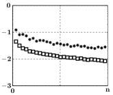
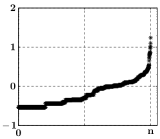
(a) Flare

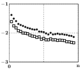
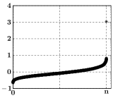
(b) Eye

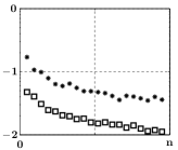
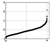
(c) BioDeg

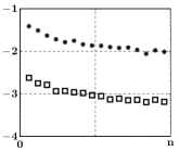
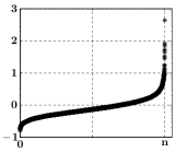
(d) Abalone

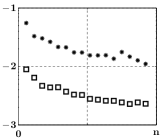
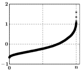
(e) Wilt

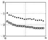
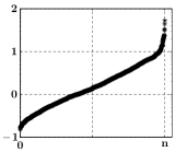
(f) Wine Red

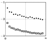
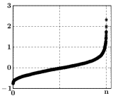
(g) Wine White

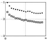
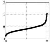
(h) Yeast

Fig. 1: Relative errors due to randomization, and ratios of leverage score over “optimal” probabilities for the matrices in Table 4. Plots in columns 1 and 3: The average over 100 runs of $\left\|\mathbf{X}-\mathbf{A}\mathbf{A}^{T}\right\|_{2}/\left\|\mathbf{A}\mathbf{A}^{T}\right\|_{2}$ when Algorithm 1 samples with “optimal probabilities” $(\square)$ and with leverage score probabilities $(*)$, versus the number $c$ of sampled columns in $\mathbf{X}$. The vertical axes are logarithmic, and the labels correspond to powers of 10. Plots in columns 2 and 4: Ratios $p_{j}^{lev}/p_{j}^{opt}$, $1\leq j\leq n$, sorted in increasing magnitude from left to right.

4 Error due to randomization, for sampling with “nearly optimal” probabilities

We present two new probabilistic bounds (Sections 4.1 and 4.2) for the two-norm relative error due to randomization, when Algorithm 1 samples with the “nearly optimal” probabilities in (2). The bounds depend on the stable rank or the rank of $\mathbf{A}$, but not on the matrix dimensions. Neither bound is always better than the other (Section 4.3). The numerical experiments (Section 4.4) illustrate that the bounds are informative, even for stringent success probabilities and matrices of small dimension.

4.1 First bound

The first bound depends on the stable rank of $\mathbf{A}$ and also, weakly, on the rank.

Theorem 10.

Let $\mathbf{A}\neq\mathbf{0}$ be an $m\times n$ matrix, and let $\mathbf{X}$ be computed by Algorithm 1 with the “nearly optimal” probabilities $p_{j}^{\beta}$ in (2).

Given $0<\delta<1$ and $0<\epsilon\leq 1$, if the number of columns sampled by Algorithm 1 is at least

$$c\geq c_{0}(\epsilon)\>\mathsf{sr}(\mathbf{A})\>\frac{\ln{(\mathop{\operator@font rank}\nolimits(\mathbf{A})/\delta)}}{\beta\,\epsilon^{2}},\qquad where\quad c_{0}(\epsilon)\equiv 2+\frac{2\epsilon}{3},$$

then with probability at least $1-\delta$,

$$\frac{\left\|\mathbf{X}-\mathbf{A}\mathbf{A}^{T}\right\|_{2}}{\|\mathbf{A}\mathbf{A}^{T}\|_{2}}\leq\epsilon.$$

Proof.

See Section 7.5. ∎

As the required error $\epsilon$ becomes smaller, so does the constant $c_{0}(\epsilon)$ in the lower bound for the number of samples, that is, $c_{0}(\epsilon)\rightarrow 2$ as $\epsilon\rightarrow 0$.

4.2 Second bound

This bound depends only on the stable rank of $\mathbf{A}$.

Theorem 11.

Let $\mathbf{A}\neq\mathbf{0}$ be an $m\times n$ matrix, and let $\mathbf{X}$ be computed by Algorithm 1 with the “nearly optimal” probabilities $p_{j}^{\beta}$ in (2).

Given $0<\delta<1$ and $0<\epsilon\leq 1$, if the number of columns sampled by Algorithm 1 is at least

$$c\geq c_{0}(\epsilon)\>\mathsf{sr}(\mathbf{A})\>\frac{\ln{(4\mathsf{sr}(\mathbf{A})/\delta)}}{\beta\,\epsilon^{2}},\qquad\mbox{where}\quad c_{0}(\epsilon)\equiv 2+\frac{2\epsilon}{3},$$

then with probability at least $1-\delta$,

$$\frac{\left\|\mathbf{X}-\mathbf{A}\mathbf{A}^{T}\right\|_{2}}{\|\mathbf{A}\mathbf{A}^{T}\|_{2}}\leq\epsilon.$$

Proof.

See Section 7.6. ∎

4.3 Comparison

The bounds in Theorems 10 and 11 differ only in the arguments of the logarithms.

On the one hand, Theorem 11 is tighter than Theorem 10 if $4\>\mathsf{sr}(\mathbf{A})<\mathop{\operator@font rank}\nolimits(\mathbf{A})$. On the other hand, Theorem 10 is tighter for matrices with large stable rank, and in particular for matrices $\mathbf{A}$ with orthonormal rows where $\mathsf{sr}(\mathbf{A})=\mathop{\operator@font rank}\nolimits(\mathbf{A})$.

In general, Theorem 11 is tighter than all the bounds in Table 2, that is, to our knowledge, all published bounds.

Matrix	$m\times n$	$\mathop{\operator@font rank}\nolimits(\mathbf{A})$	$\mathsf{sr}(\mathbf{A})$	$c\,\gamma_{1}$	$c\,\gamma_{2}$
us04	$163\times 28016$	115	5.27	16.43	13.44
bibd_16_8	$163\times 28016$	120	4.29	13.43	10.65

Table 5: Matrices from [15], their dimensions, rank and stable rank; and key quantities from (4) and (5).

4.4 Numerical experiments

We compare the bounds in Theorems 10 and 11 to the errors of Algorithm 1 for sampling with “optimal” probabilities.

Experimental set up

We present experiments with two matrices from the University of Florida Sparse Matrix Collection [15]. The matrices have the same dimension, and similar high ranks and low stable ranks, see Table 5. Note that only for low stable ranks can Algorithm 1 achieve any accuracy.

The sampling amounts $c$ range from 1 to $n$, the number of columns, with 100 runs for each value of $c$. From the 100 errors $\|\mathbf{X}-\mathbf{A}\mathbf{A}^{T}\|_{2}/\|\mathbf{A}\mathbf{A}^{T}\|_{2}$ for each $c$ value, we plot the smallest, largest, and average.

In Theorems 10 and 11, the success probability is 99 percent, that is, a failure probability of $\delta=.01$. The error bounds are plotted as a function of $c$. That is, for Theorem 10 we plot (see Theorem 22)

$$\frac{\left\|\mathbf{X}-\mathbf{A}\mathbf{A}^{T}\right\|_{2}}{\|\mathbf{A}\mathbf{A}^{T}\|_{2}}\leq\gamma_{1}+\sqrt{\gamma_{1}\>(6+\gamma_{1})},\qquad\gamma_{1}\equiv\mathsf{sr}(\mathbf{A})\>\frac{\ln{(\mathop{\operator@font rank}\nolimits(\mathbf{A})/.01)}}{3\,\,c}$$ (4)

while for Theorem 11 we plot (see Theorem 24)

$$\frac{\left\|\mathbf{X}-\mathbf{A}\mathbf{A}^{T}\right\|_{2}}{\|\mathbf{A}\mathbf{A}^{T}\|_{2}}\leq\gamma_{2}+\sqrt{\gamma_{2}\>(6+\gamma_{2})},\qquad\gamma_{2}\equiv\>\mathsf{sr}(\mathbf{A})\>\frac{\ln{(4\mathsf{sr}(\mathbf{A})/.01)}}{3\,c}$$ (5)

The key quantities $c\>\gamma_{1}$ and $c\>\gamma_{2}$ are shown for both matrices in Table 5.

Figure 2 contains two plots, the left one for matrix us04, and the right one for matrix bibd_16_8. The plots show the relative errors $\|\mathbf{X}-\mathbf{A}\mathbf{A}^{T}\|_{2}/\|\mathbf{A}\mathbf{A}^{T}\|_{2}$ and the bounds (4) and (5) versus the sampling amount $c$.

Conclusions

In both plots, the bounds corresponding to Theorems 10 and 11 are virtually indistinguishable, as was is already predicted by the key quantities $c\>\gamma_{1}$ and $c\>\gamma_{2}$ in Table 5. The bounds overestimate the worst case error from Algorithm 1 by a factor of at most 10. Hence they are informative, even for matrices of small dimension and a stringent success probability.

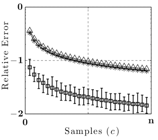
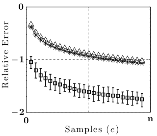
Fig. 2: Relative errors due to randomization from Algorithm 1, and bounds (4) and (5) versus sampling amount $c$, for matrices us04 (left) and bidb_16_8 (right). Error bars represent the maximum and minimum of the errors $\left\|\mathbf{X}-\mathbf{A}\mathbf{A}^{T}\right\|_{2}/\left\|\mathbf{A}\mathbf{A}^{T}\right\|_{2}$ from Algorithm 1 over 100 runs, while the squares represent the average. The triangles $(\bigtriangleup)$ represent the bound (4), while the stars $(*)$ represent (5). The vertical axes are logarithmic, and the labels correspond to powers of 10.

5 Error due to randomization, for sampling with leverage score probabilities

For completeness, we present a normwise relative bound for the error due to randomization, when Algorithm 1 samples with leverage score probabilities (3). The bound corroborates the numerical experiments in Section 3.2.3, and suggests that sampling with leverage score probabilities produces a larger error due to randomization than sampling with “nearly optimal” probabilities.

Theorem 12.

Let $\mathbf{A}\neq\mathbf{0}$ be an $m\times n$ matrix, and let $\mathbf{X}$ be computed by Algorithm 1 with the leverage score probabilites $p_{j}^{lev}$ in (3).

Given $0<\delta<1$ and $0<\epsilon\leq 1$, if the number of columns sampled by Algorithm 1 is at least

$$c\geq c_{0}(\epsilon)\>\mathop{\operator@font rank}\nolimits(\mathbf{A})\>\frac{\ln(\mathop{\operator@font rank}\nolimits(\mathbf{A})/\delta)}{\epsilon^{2}},\qquad\mbox{where}\quad c_{0}(\epsilon)=2+\frac{2\epsilon}{3},$$

then with probability at least $1-\delta$,

$$\frac{\left\|\mathbf{X}-\mathbf{A}\mathbf{A}^{T}\right\|_{2}}{\left\|\mathbf{A}\mathbf{A}^{T}\right\|_{2}}\leq\epsilon.$$

Proof.

See Section 7.7. ∎

In the special case when $\mathbf{A}$ has orthonormal columns, the leverage score probabilities $p_{j}^{lev}$ are equal to the “optimal” probabilities $p_{j}^{opt}$ in (1). Furthermore, $\mathop{\operator@font rank}\nolimits(\mathbf{A})=\mathsf{sr}(\mathbf{A})$, so that Theorem 12 is equal to Theorem 10. For general matrices $\mathbf{A}$, though, $\mathop{\operator@font rank}\nolimits(\mathbf{A})\geq\mathsf{sr}(\mathbf{A})$, and Theorem 12 is not as tight as Theorem 10.

6 Singular value and condition number bounds

As in [21], we apply the bounds for the Gram matrix approximation to a matrix with orthonormal rows, and derive bounds for the smallest singular value (Section 6.1) and condition number (Section 6.2) of a sampled matrix.

Specifically, let $\mathbf{Q}$ be a real $m\times n$ matrix with orthonormal rows, $\mathbf{Q}\mathbf{Q}^{T}=\mathbf{I}_{m}$. Then, as discussed in Section 3.2.1, the “optimal” probabilities (1) for $\mathbf{Q}$ are equal to the leverage score probabilities (3),

$$p_{j}^{opt}=\frac{\|Q_{j}\|_{2}^{2}}{\|\mathbf{Q}\|_{F}^{2}}=\frac{\|Q_{j}\|_{2}^{2}}{m}=p_{j}^{lev},\qquad 1\leq j\leq m.$$

The connection between Gram matrix approximations $(\mathbf{Q}\mathbf{S})\>(\mathbf{Q}\mathbf{S})^{T}$ and singular values of the sampled matrix $\mathbf{Q}\mathbf{S}$ comes from the well-conditioning of singular values [30, Corollary 2.4.4],

$$\left|1-\sigma_{j}\left(\mathbf{Q}\mathbf{S}\right)^{2}\right| = \left|\sigma_{j}\left(\mathbf{Q}\mathbf{Q}^{T}\right)-\sigma_{j}\left((\mathbf{Q}\mathbf{S})\>(\mathbf{Q}\mathbf{S})^{T}\right)\right|$$ (6)

$$\leq \left\|\mathbf{Q}\mathbf{Q}^{T}-(\mathbf{Q}\mathbf{S})\>(\mathbf{Q}\mathbf{S})^{T}\right\|_{2},\qquad 1\leq j\leq m.$$

6.1 Singular value bounds

We present two bounds for the smallest singular value of a sampled matrix, for sampling with the “nearly optimal” probabilities (2), and for uniform sampling with and without replacement.

The first bound is based on the Gram matrix approximation in Theorem 10.

Theorem 13.

Let $\mathbf{Q}$ be an $m\times n$ matrix with orthonormal rows and coherence $\mu$, and let $\mathbf{Q}\mathbf{S}$ be computed by Algorithm 1. Given $0<\epsilon<1$ and $0<\delta<1$, we have $\sigma_{m}\left(\mathbf{Q}\mathbf{S}\right)\geq\sqrt{1-\epsilon}$ with probability at least $1-\delta$, if Algorithm 1

• either samples with the “nearly optimal” probabilities $p_{j}^{\beta}$, and

  $$c\geq c_{0}(\epsilon)\>m\>\frac{\ln(m/\delta)}{\beta\epsilon^{2}},$$

• or samples with uniform probabilities $1/n$, and

  $$c\geq c_{0}(\epsilon)\>n\,\mu\>\frac{\ln(m/\delta)}{\epsilon^{2}}.$$

Here $c_{0}(\epsilon)\equiv 2+\tfrac{2}{3}\>\epsilon$.

Proof.

See Section 7.8. ∎

Since $c_{0}(\epsilon)\geq 2$, the above bound for uniform sampling is slightly less tight than the last bound in Table 3, i.e. [26, Lemma 1]. Although that bound technically holds only for uniform sampling without replacement, the same proof gives the same bound for uniform sampling with replacement.

This inspired us to derive a second bound, by modifying the argument in [26, Lemma 1], to obtain a slightly tighter constant. This is done with a direct application of a Chernoff bound (Theorem 25). The only difference between the next and the previous result is the smaller constant $c_{1}(\epsilon)$, and the added application to sampling without replacement.

Theorem 14.

Let $\mathbf{Q}$ be an $m\times n$ matrix with orthonormal rows and coherence $\mu$, and let $\mathbf{Q}\mathbf{S}$ be computed by Algorithm 1. Given $0<\epsilon<1$ and $0<\delta<1$, we have $\sigma_{m}\left(\mathbf{Q}\mathbf{S}\right)\geq\sqrt{1-\epsilon}$ with probability at least $1-\delta$, if Algorithm 1

• either samples with the “nearly optimal” probabilities $p_{j}^{\beta}$, and

  $$c\geq c_{1}(\epsilon)\>m\>\frac{\ln(m/\delta)}{\beta\epsilon^{2}},$$

• or samples with uniform probabilities $1/n$, with or without replacement, and

  $$c\geq c_{1}(\epsilon)\>n\,\mu\>\frac{\ln(m/\delta)}{\epsilon^{2}}.$$

Here $c_{1}(\epsilon)\equiv\tfrac{\epsilon^{2}}{(1-\epsilon)\ln(1-\epsilon)+\epsilon}$, and $1\leq c_{1}(\epsilon)\leq 2$.

Proof.

See Section 7.9. ∎

The constant $c_{1}(\epsilon)$ is slightly smaller than the constant 2 in [26, Lemma 1], which is the last bound in Table 3.

6.2 Condition number bounds

We present two bounds for the condition number $\kappa(\mathbf{Q}\mathbf{S})\equiv\sigma_{1}(\mathbf{Q}\mathbf{S})/\sigma_{m}(\mathbf{Q}\mathbf{S})$ of a sampled matrix $\mathbf{Q}\mathbf{S}$ with full row-rank.

The first condition number bound is based on a Gram matrix approximation, and is analogous to Theorem 13.

Theorem 15.

Let $\mathbf{Q}$ be an $m\times n$ matrix with orthonormal rows and coherence $\mu$, and let $\mathbf{Q}\mathbf{S}$ be computed by Algorithm 1. Given $0<\epsilon<1$ and $0<\delta<1$, we have $\kappa(\mathbf{Q}\mathbf{S})\leq\tfrac{\sqrt{1+\epsilon}}{\sqrt{1-\epsilon}}$ with probability at least $1-\delta$, if Algorithm 1

• either samples with the “nearly optimal” probabilities $p_{j}^{\beta}$, and

  $$c\geq c_{0}(\epsilon)\>m\>\frac{\ln(m/\delta)}{\beta\epsilon^{2}},$$

• or samples with uniform probabilities $1/n$, and

  $$c\geq c_{0}(\epsilon)\>n\,\mu\>\frac{\ln(m/\delta)}{\epsilon^{2}}.$$

Here $c_{0}(\epsilon)\equiv 2+\tfrac{2}{3}\>\epsilon$.

Proof.

See Section 7.10. ∎

The second condition number bound is based on a Chernoff inequality, and is analogous to Theorem 14, but with a different constant, and an additional factor of two in the logarithm.

Theorem 16.

Let $\mathbf{Q}$ be an $m\times n$ matrix with orthonormal rows and coherence $\mu$, and let $\mathbf{Q}\mathbf{S}$ be computed by Algorithm 1. Given $0<\epsilon<1$ and $0<\delta<1$, we have $\kappa(\mathbf{Q}\mathbf{S})\leq\tfrac{\sqrt{1+\epsilon}}{\sqrt{1-\epsilon}}$ with probability at least $1-\delta$, if Algorithm 1

• either samples with the “nearly optimal” probabilities $p_{j}^{\beta}$, and

  $$c\geq c_{2}(\epsilon)\>m\>\frac{\ln(2m/\delta)}{\beta\epsilon^{2}},$$

• or samples with uniform probabilities $1/n$, with or without replacement, and

  $$c\geq c_{2}(\epsilon)\>n\,\mu\>\frac{\ln(2m/\delta)}{\epsilon^{2}}.$$

Here $c_{2}(\epsilon)\equiv\tfrac{\epsilon^{2}}{(1+\epsilon)\ln(1+\epsilon)-\epsilon}$, and $2\leq c_{2}(\epsilon)\leq 2.6$.

Proof.

See Section 7.11. ∎

It is difficult to compare the two condition number bounds, and neither bound is always tighter than the other. On the one hand, Theorem 16 has a smaller constant than Theorem 15 since $c_{2}(\epsilon)\leq c_{1}(\epsilon)$. On the other hand, though, Theorem 15 has an additional factor of two in the logarithm. For very large $m/\delta$, the additional factor of 2 in the logarithm does not matter much and Theorem 16 is tighter.

In general, Theorem 16 is not always tighter than Theorem 15. For example, if $m=100$, $\delta=0.01$, $\epsilon=0.1$, $\beta=1$, and Algorithm 1 samples with “nearly optimal” probabilities, then Theorem 16 requires $1.57\cdot 10^{5}$ samples, while Theorem 15 requires only $1.43\cdot 10^{5}$; hence, it is tighter.

7 Proofs

We present proofs for the results in Sections 2 – 6.

7.1 Proof of Theorem 1

We will use the two lemmas below. The first one is a special case of [23, Theorem 2.1] where the rank of the approximation is not restricted.

Lemma 17.

Let $\mathbf{H}$ be $m\times n$, $\mathbf{B}$ be $m\times p$, and $\mathbf{C}$ be $q\times n$ matrices, and let $\mathbf{P}_{\mathbf{B}}$ be the orthogonal projector onto $\mathsf{range}(\mathbf{B})$, and $\mathbf{P}_{\mathbf{C}^{T}}$ the orthogonal projector onto $\mathsf{range}(\mathbf{C}^{T})$. Then the solution of

$$\min_{\mathbf{W}}{\|\mathbf{H}-\mathbf{B}\,\mathbf{W}\,\mathbf{C}\|_{F}}$$

with minimal Frobenius norm is

$$\mathbf{W}=\mathbf{B}^{\dagger}\>\mathbf{P}_{\mathbf{B}}\,\mathbf{H}\,\mathbf{P}_{\mathbf{C}^{T}}\>\mathbf{C}^{\dagger}.$$

Lemma 18.

If $\mathbf{B}$ is $m\times p$ and $\mathbf{C}$ is $p\times n$, with $\mathop{\operator@font rank}\nolimits(\mathbf{B})=p=\mathop{\operator@font rank}\nolimits(\mathbf{C})$, then $(\mathbf{B}\mathbf{C})^{\dagger}=\mathbf{C}^{\dagger}\mathbf{B}^{\dagger}$.

Proof.

Set $\mathbf{Y}\equiv\mathbf{B}\mathbf{C}$, and use $\mathbf{B}^{\dagger}\mathbf{B}=\mathbf{I}_{p}=\mathbf{C}\mathbf{C}^{\dagger}$ to verify that $\mathbf{Z}\equiv\mathbf{C}^{\dagger}\mathbf{B}^{\dagger}$ satisfies the four conditions defining the Moore-Penrose inverse

$$\mathbf{Y}\mathbf{Z}\mathbf{Y}=\mathbf{Y},\quad\mathbf{Z}\mathbf{Y}\mathbf{Z}=\mathbf{Z},\quad(\mathbf{Y}\mathbf{Z})^{T}=\mathbf{Y}\mathbf{Z},\quad(\mathbf{Z}\mathbf{Y})^{T}=\mathbf{Z}\mathbf{Y}.$$ (7)

∎

Proof of Theorem 1

Abbreviate $\mathbf{A}_{1}\equiv\mathbf{A}\mathbf{S}$ and $\mathbf{V}_{1}^{T}\equiv\mathbf{V}^{T}\mathbf{S}$.

In Lemma 17, set $\mathbf{H}=\mathbf{A}\mathbf{A}^{T}$, $\mathbf{B}=\mathbf{A}_{1}$, and $\mathbf{C}=\mathbf{A}_{1}^{T}$. Then $\mathbf{P}_{\mathbf{B}}=\mathbf{A}_{1}\mathbf{A}_{1}^{\dagger}=\mathbf{P}_{\mathbf{C}^{T}}$, and

$$\mathbf{W}_{opt}=\mathbf{A}_{1}^{\dagger}\>\mathbf{A}_{1}\mathbf{A}_{1}^{\dagger}\,\mathbf{A}\mathbf{A}^{T}\,\mathbf{A}_{1}\mathbf{A}_{1}^{\dagger}\>(\mathbf{A}_{1}^{\dagger})^{T}.$$

The conditions for the Moore-Penrose inverse (7) imply $\mathbf{A}_{1}^{\dagger}\mathbf{A}_{1}\mathbf{A}_{1}^{\dagger}=\mathbf{A}_{1}^{\dagger}$, and

$$\mathbf{A}_{1}\mathbf{A}_{1}^{\dagger}\>(\mathbf{A}_{1}^{\dagger})^{T}=\left(\mathbf{A}_{1}\mathbf{A}_{1}^{\dagger}\right)^{T}\>(\mathbf{A}_{1}^{\dagger})^{T}=(\mathbf{A}_{1}^{\dagger})^{T}\>\mathbf{A}_{1}^{T}\>(\mathbf{A}_{1}^{\dagger})^{T}=(\mathbf{A}_{1}^{\dagger})^{T}.$$

Hence $\mathbf{W}_{opt}=\mathbf{A}_{1}^{\dagger}\>\mathbf{A}\mathbf{A}^{T}\>(\mathbf{A}_{1}^{\dagger})^{T}$.

Special case $\mathop{\operator@font rank}\nolimits(\mathbf{A}_{1})=\mathop{\operator@font rank}\nolimits(\mathbf{A})$

This means the number of columns $c$ in $\mathbf{A}_{1}=\mathbf{U}\mathbf{\Sigma}\mathbf{V}_{1}^{T}$ is at least as large as $k\equiv\mathop{\operator@font rank}\nolimits(\mathbf{A})$. Hence $\mathbf{V}_{1}^{T}$ is $k\times c$ with $c\geq k$, and $\mathop{\operator@font rank}\nolimits(\mathbf{V}_{1}^{T})=k=\mathop{\operator@font rank}\nolimits(\mathbf{U}\mathbf{\Sigma})$. From Lemma 18 follows $\mathbf{A}_{1}^{\dagger}=(\mathbf{V}_{1}^{\dagger})^{T}\>\mathbf{\Sigma}^{-1}\mathbf{U}^{T}$. Hence

$$\mathbf{W}_{opt}=(\mathbf{V}_{1}^{\dagger})^{T}\>\mathbf{V}^{T}\mathbf{V}\>\mathbf{V}_{1}^{\dagger}=(\mathbf{V}_{1}^{\dagger})^{T}\>\mathbf{V}_{1}^{\dagger}.$$

Furthermore $\mathop{\operator@font rank}\nolimits(\mathbf{A}_{1})=\mathop{\operator@font rank}\nolimits(\mathbf{A})$ implies that $\mathbf{A}_{1}$ has the same column space as $\mathbf{A}$. Hence the residual in Theorem 1 is zero, and $\mathbf{A}_{1}\mathbf{W}_{opt}\mathbf{A}_{1}^{T}=\mathbf{A}\mathbf{A}^{T}$.

Special case $c=\mathop{\operator@font rank}\nolimits(\mathbf{A}_{1})=\mathop{\operator@font rank}\nolimits(\mathbf{A})$

This means $c=k$, so that $\mathbf{V}_{1}$ is a $k\times k$ matrix. From $\mathop{\operator@font rank}\nolimits(\mathbf{A})=k$ follows $\mathop{\operator@font rank}\nolimits(\mathbf{V}_{1})=k$, so that $\mathbf{V}_{1}$ is nonsingular and $\mathbf{V}_{1}^{\dagger}=\mathbf{V}_{1}^{-1}$.

7.2 Proof of Theorem 2

Abbreviate

$$\mathbf{A}_{1}\equiv\begin{pmatrix}A_{t_{1}}&\cdots&A_{t_{c}}\end{pmatrix},\qquad\mathbf{V}_{1}^{T}\equiv\mathbf{V}^{T}\begin{pmatrix}e_{t_{1}}&\cdots&e_{t_{c}}\end{pmatrix},$$

so that the sum of outer products can be written as $\sum_{j=1}^{c}{w_{j}\>A_{t_{j}}A_{t_{j}}^{T}}=\mathbf{A}_{1}\mathbf{W}\mathbf{A}_{1}^{T}$, where $\mathbf{W}\equiv\mathop{\operator@font diag}\nolimits\begin{pmatrix}w_{1}&\cdots&w_{c}\end{pmatrix}$.

1. Show: If $\mathbf{A}_{1}\mathbf{W}\mathbf{A}_{1}^{T}=\mathbf{A}\mathbf{A}^{T}$ for a diagonal $\mathbf{W}$ with non-negative diagonal, then $\mathbf{V}_{1}^{T}\mathbf{W}^{1/2}$ has orthonormal rows

From $\mathbf{A}\mathbf{A}^{T}=\mathbf{A}_{1}\mathbf{W}\mathbf{A}_{1}^{T}$ follows

$$\mathbf{U}\mathbf{\Sigma}^{2}\mathbf{U}^{T}=\mathbf{A}\mathbf{A}^{T}=\mathbf{A}_{1}\mathbf{W}\mathbf{A}_{1}^{T}=\mathbf{U}\mathbf{\Sigma}\>\mathbf{V}_{1}^{T}\,\mathbf{W}\,\mathbf{V}_{1}\>\mathbf{\Sigma}\mathbf{U}^{T}.$$ (8)

Multiplying by $\mathbf{\Sigma}^{-1}\mathbf{U}^{T}$ on the left and by $\mathbf{U}\mathbf{\Sigma}^{-1}$ on the right gives $\mathbf{I}_{k}=\mathbf{V}_{1}^{T}\,\mathbf{W}\,\mathbf{V}_{1}$. Since $\mathbf{W}$ is positive semi-definite, it has a symmetric positive semi-definite square root $\mathbf{W}^{1/2}$. Hence $\mathbf{I}_{k}=\mathbf{V}_{1}^{T}\,\mathbf{W}\,\mathbf{V}_{1}=(\mathbf{V}_{1}^{T}\mathbf{W}^{1/2})\>(\mathbf{V}_{1}^{T}\mathbf{W}^{1/2})^{T}$, and $\mathbf{V}_{1}^{T}\mathbf{W}^{1/2}$ has orthonormal rows.

2. Show: If $\mathbf{V}_{1}^{T}\mathbf{W}^{1/2}$ has orthonormal rows, then $\mathbf{A}_{1}\mathbf{W}\mathbf{A}_{1}^{T}=\mathbf{A}\mathbf{A}^{T}$

Inserting $\mathbf{I}_{k}=(\mathbf{V}_{1}^{T}\mathbf{W}^{1/2})\>(\mathbf{V}_{1}^{T}\mathbf{W}^{1/2})^{T}=\mathbf{V}_{1}^{T}\mathbf{W}\mathbf{V}_{1}$ into $\mathbf{A}_{1}\mathbf{W}\mathbf{A}_{1}^{T}$ gives

$$\mathbf{A}_{1}\mathbf{W}\mathbf{A}_{1}^{T}=\mathbf{U}\mathbf{\Sigma}\>\left(\mathbf{V}_{1}^{T}\,\mathbf{W}\,\mathbf{V}_{1}\right)\>\mathbf{\Sigma}\mathbf{U}^{T}=\mathbf{U}\mathbf{\Sigma}^{2}\mathbf{U}^{T}=\mathbf{A}\mathbf{A}^{T}.$$

7.3 Proof of Corollary 3

Since $\mathop{\operator@font rank}\nolimits(\mathbf{A})=1$, the right singular vector matrix $\mathbf{V}=\begin{pmatrix}v_{1}&\ldots&v_{n}\end{pmatrix}^{T}$ is a $n\times 1$ vector. Since $\mathbf{A}$ has only a single non-zero singular value, $\|A_{j}\|_{2}=\|\mathbf{U}\mathbf{\Sigma}\>v_{j}\|_{2}=\|\mathbf{A}\|_{F}v_{j}$. Clearly $A_{j}\neq 0$ if and only $v_{j}\neq 0$, and $\|\mathbf{V}^{T}e_{j}\|_{2}^{2}=v_{j}^{2}=\|A_{j}\|_{2}^{2}/\|\mathbf{A}\|_{F}^{2}$. Let $A_{t_{j}}$ be any $c$ non-zero columns of $\mathbf{A}$. Then

$$\sum_{j=1}^{c}{w_{j}A_{t_{j}}A_{t_{j}}^{T}}=\mathbf{U}\mathbf{\Sigma}\>\left(\sum_{j=1}^{c}{w_{j}v_{t_{j}}^{2}}\right)\>\mathbf{\Sigma}\mathbf{U}^{T}=\mathbf{U}\mathbf{\Sigma}^{2}\mathbf{U}^{T}=\mathbf{A}\mathbf{A}^{T}$$

if and only if $\sum_{j=1}^{c}{w_{j}v_{t_{j}}^{2}}=1$. This is true if $w_{j}=1/(cv_{t_{j}}^{2})$, $1\leq j\leq c$.

7.4 Proof of Theorem 6

Since Theorem 6 is a special case of Theorem 2, we only need to derive the expression for the weights. From $c=k$ follows that $\mathbf{V}_{1}^{T}\mathbf{W}^{1/2}$ is $k\times k$ with orthonormal rows. Hence $\mathbf{V}_{1}^{T}\mathbf{W}^{1/2}$ is an orthogonal matrix, and must have orthonormal columns as well, $(\mathbf{W}^{1/2}\mathbf{V}_{1})\>(\mathbf{W}^{1/2}\mathbf{V}_{1})^{T}=\mathbf{I}_{k}$. Thus

$$\mathbf{V}_{1}\mathbf{V}_{1}^{T}=\mathop{\operator@font diag}\nolimits\begin{pmatrix}\left\|\mathbf{V}^{T}e_{t_{1}}\right\|_{2}^{2}&\cdots&\left\|\mathbf{V}^{T}e_{t_{c}}\right\|_{2}^{2}\end{pmatrix}=\mathbf{W}^{-1}.$$

This and $\mathbf{W}^{1/2}$ being diagonal implies $w_{j}=1/\left\|\mathbf{V}^{T}e_{t_{j}}\right\|_{2}^{2}$.

7.5 Proof of Theorem 10

We present two auxiliary results, a matrix Bernstein concentration inequality (Theorem 19) and a bound for the singular values of a difference of positive semi-definite matrices (Theorem 20), before deriving a probabilistic bound (Theorem 21). The subsequent combination of Theorem 21 and the invariance of the two-norm under unitary transformations yields Theorem 22 which, at last, leads to a proof for the desired Theorem 10.

Theorem 19 (Theorem 1.4 in [51]).

Let $\mathbf{X}_{j}$ be $c$ independent real symmetric random $m\times m$ matrices. Assume that, with probability one, $\mathbb{E}[\mathbf{X}_{j}]=\mathbf{0}$, $1\leq j\leq c$ and $\max_{1\leq j\leq c}{\|\mathbf{X}_{j}\|_{2}}\leq\rho_{1}$. Let $\left\|\sum_{j=1}^{c}{\mathbb{E}[\mathbf{X}_{j}^{2}]}\right\|_{2}\leq\rho_{2}$.

Then for any $\epsilon\geq 0$

$$\mathbb{P}\left[\left\|\sum_{j=1}^{c}{\mathbf{X}_{j}}\right\|_{2}\geq\epsilon\right]\leq m\>\exp\left(-\frac{\epsilon^{2}/2}{\rho_{2}+\rho_{1}\epsilon/3}\right).$$

Theorem 20 (Theorem 2.1 in [54]).

If $\mathbf{B}$ and $\mathbf{C}$ are $m\times m$ real symmetric positive semi-definite matrices, with singular values $\sigma_{1}(\mathbf{B})\geq\ldots\geq\sigma_{m}(\mathbf{B})$ and $\sigma_{1}(\mathbf{C})\geq\ldots\geq\sigma_{m}(\mathbf{C})$, then the singular values of the difference are bounded by

$$\sigma_{j}(\mathbf{B}-\mathbf{C})\leq\sigma_{j}\begin{pmatrix}\mathbf{B}&\mathbf{0}\\ \mathbf{0}&\mathbf{C}\end{pmatrix},\qquad 1\leq j\leq m.$$

In particular, $\|\mathbf{B}-\mathbf{C}\|_{2}\leq\max\{\|\mathbf{B}\|_{2},\,\|\mathbf{C}\|_{2}\}$.

Theorem 21.

Let $\mathbf{A}\neq\mathbf{0}$ be an $m\times n$ matrix, and let $\mathbf{X}$ be computed by Algorithm 1 with the “nearly optimal” probabilites $p_{j}^{\beta}$ in (2).

For any $\delta>0$, with probability at least $1-\delta$,

$$\frac{\left\|\mathbf{X}-\mathbf{A}\mathbf{A}^{T}\right\|_{2}}{\|\mathbf{A}\mathbf{A}^{T}\|_{2}}\leq\gamma_{0}+\sqrt{\gamma_{0}\>(6+\gamma_{0})},\qquad where\quad\gamma_{0}\equiv\mathsf{sr}(\mathbf{A})\>\frac{\ln{(m/\delta)}}{3\,\beta\,c}.$$

Proof.

In order to apply Theorem 19, we need to change variables, and check that the assumptions are satisfied.

1. Change of variables

Define the $m\times m$ real symmetric matrix random variables $\mathbf{Y}_{j}\equiv\frac{1}{c\,p_{t_{j}}}\>A_{t_{j}}A_{t_{j}}^{T}$, and write the output of Algorithm 1 as

$$\mathbf{X}=(\mathbf{A}\mathbf{S})\>(\mathbf{A}\mathbf{S})^{T}=\mathbf{Y}_{1}+\cdots+\mathbf{Y}_{c}.$$

Since $\mathbb{E}[\mathbf{Y}_{j}]=\mathbf{A}\mathbf{A}^{T}/c$, but Theorem 19 requires random variables with zero mean, set $\mathbf{X}_{j}\equiv\mathbf{Y}_{j}-\frac{1}{c}\mathbf{A}\mathbf{A}^{T}$. Then

$$\mathbf{X}-\mathbf{A}\mathbf{A}^{T}=(\mathbf{A}\mathbf{S})\,(\mathbf{A}\mathbf{S})^{T}-\mathbf{A}\mathbf{A}^{T}=\sum_{j=1}^{c}{\left(\mathbf{Y}_{j}-\frac{1}{c}\,\mathbf{A}\mathbf{A}^{T}\right)}=\sum_{j=1}^{c}{\mathbf{X}_{j}}.$$

Hence, we show $\left\|\mathbf{X}-\mathbf{A}\mathbf{A}^{T}\right\|_{2}\leq\epsilon$ by showing $\left\|\sum_{j=1}^{c}{\mathbf{X}_{j}}\right\|_{2}\leq\epsilon$.

Next we have to check that the assumptions of Theorem 19 are satisfied. In order to derive bounds for $\max_{1\leq j\leq c}{\|\mathbf{X}_{j}\|_{2}}$ and $\left\|\sum_{j=1}^{c}{\mathbb{E}[\mathbf{X}_{j}^{2}]}\right\|_{2}$, we assume general non-zero probabilities $p_{j}$ for the moment, that is, $p_{j}>0$, $1\leq j\leq n$.

2. Bound for $\max_{1\leq j\leq c}{\|\mathbf{X}_{j}\|_{2}}$

Since $\mathbf{X}_{j}$ is a difference of positive semidefinite matrices, apply Theorem 20 to obtain

$$\|\mathbf{X}_{j}\|_{2}\leq\max\left\{\|\mathbf{Y}_{j}\|_{2},\,\tfrac{1}{c}\left\|\mathbf{A}\mathbf{A}^{T}\right\|_{2}\right\}\leq\frac{\hat{\rho}_{1}}{c},\qquad\hat{\rho}_{1}\equiv\max_{1\leq i\leq n}\left\{\frac{\|A_{i}\|_{2}^{2}}{p_{i}},\,\left\|\mathbf{A}\right\|_{2}^{2}\right\}.$$

3. Bound for $\left\|\sum_{j=1}^{c}{\mathbb{E}[\mathbf{X}_{j}^{2}]}\right\|_{2}$

To determine the expected value of

$$\mathbf{X}_{j}^{2}=\mathbf{Y}_{j}^{2}-\tfrac{1}{c}\,\mathbf{A}\mathbf{A}^{T}\>\mathbf{Y}_{j}-\tfrac{1}{c}\mathbf{Y}_{j}\>\mathbf{A}\mathbf{A}^{T}+\tfrac{1}{c^{2}}(\mathbf{A}\mathbf{A}^{T})^{2}$$

use the linearity of the expected value and $\mathbb{E}[\mathbf{Y}_{j}]=\mathbf{A}\mathbf{A}^{T}/c$ to obtain

$$\mathbb{E}[\mathbf{X}_{j}^{2}]=\mathbb{E}[\mathbf{Y}_{j}^{2}]-\frac{1}{c^{2}}\,(\mathbf{A}\mathbf{A}^{T})^{2}.$$

Applying the definition of expected value again yields

$$\mathbb{E}[\mathbf{Y}_{j}^{2}]=\frac{1}{c^{2}}\>\sum_{i=1}^{n}{p_{i}\>\frac{(A_{i}A_{i}^{T})^{2}}{p^{2}_{i}}}=\frac{1}{c^{2}}\>\sum_{i=1}^{n}{\frac{(A_{i}A_{i}^{T})^{2}}{p_{i}}}.$$

Hence

$$\sum_{j=1}^{c}{\mathbb{E}[\mathbf{X}_{j}^{2}]} = \frac{1}{c}\>\left(\sum_{i=1}^{n}{\frac{(A_{i}A_{i}^{T})^{2}}{p_{i}}}-(\mathbf{A}\mathbf{A}^{T})^{2}\right)=\frac{1}{c}\mathbf{A}\>\left(\sum_{i=1}^{n}{e_{i}\frac{\|A_{i}\|_{2}^{2}}{p_{i}}e_{i}^{T}}-\mathbf{A}^{T}\mathbf{A}\right)\>\mathbf{A}^{T}$$

$$= \frac{1}{c}\mathbf{A}\>(\mathbf{L}-\mathbf{A}^{T}\mathbf{A})\>\mathbf{A}^{T},$$

where $\mathbf{L}\equiv\mathop{\operator@font diag}\nolimits\begin{pmatrix}\|A_{1}\|_{2}^{2}/p_{1}&\ldots&\|A_{n}\|_{2}^{2}/p_{n}\end{pmatrix}$. Taking norms and applying Theorem 20 to $\|\mathbf{L}-\mathbf{A}^{T}\mathbf{A}\|_{2}$ gives

$$\left\|\sum_{j=1}^{c}{\mathbb{E}[\mathbf{X}_{j}^{2}]}\right\|_{2}\leq\frac{\|\mathbf{A}\|_{2}^{2}}{c}\>\max\left\{\|\mathbf{L}\|_{2},\,\|\mathbf{A}\|_{2}^{2}\right\}=\frac{\|\mathbf{A}\|_{2}^{2}}{c}\>\hat{\rho}_{1}.$$

4. Application of Theorem 19

The required upper bounds for Theorem 19 are

$$\|\mathbf{X}_{j}\|_{2}\leq\rho_{1}\equiv\frac{\hat{\rho}_{1}}{c}\qquad and\qquad\left\|\sum_{j=1}^{c}{\mathbb{E}[\mathbf{X}_{j}^{2}]}\right\|_{2}\leq\rho_{2}\equiv\frac{\|\mathbf{A}\|_{2}^{2}}{c}\>\hat{\rho}_{1}.$$

Inserting these bounds into Theorem 19 gives

$$\mathbb{P}\left[\left\|\sum_{j=1}^{c}{\mathbf{X}_{j}}\right\|_{2}>\epsilon\right]\leq m\>\exp\left(\frac{-c\epsilon^{2}}{2\hat{\rho}_{1}\,(\|\mathbf{A}\|_{2}^{2}+\epsilon/3)}\right).$$

Hence $\left\|\sum_{j=1}^{c}{\mathbf{X}_{j}}\right\|_{2}\leq\epsilon$ with probability at least $1-\delta$, where

$$\delta\equiv m\>\exp\left(\frac{-c\epsilon^{2}}{2\hat{\rho}_{1}\,(\|\mathbf{A}\|_{2}^{2}+\epsilon/3)}\right).$$

Solving for $\epsilon$ gives

$$\epsilon=\tau_{1}\,\hat{\rho}_{1}+\sqrt{\tau_{1}\,\hat{\rho}_{1}\>\left(6\|\mathbf{A}\|_{2}^{2}+\tau_{1}\,\hat{\rho}_{1}\right)},\qquad\tau_{1}\equiv\frac{\ln{(m/\delta)}}{3c}.$$

5. Specialization to “nearly optimal” probabilities

We remove zero columns from the matrix. This does not change the norm or the stable rank. The “nearly optimal” probabilities for the resulting submatrix are $p_{j}^{\beta}=\beta\|A_{j}\|_{2}^{2}/\|\mathbf{A}\|_{F}^{2}$, with $p_{j}>0$ for all $j$. Now replace $p_{j}^{\beta}$ by their lower bounds (2). This gives $\hat{\rho}_{1}\leq\|\mathbf{A}\|_{2}^{2}\,\tau_{2}$ where $\tau_{2}\equiv\mathsf{sr}(\mathbf{A})/\beta\geq 1$, and

$$\epsilon\leq\|\mathbf{A}\|_{2}^{2}\left(\tau_{1}\tau_{2}+\sqrt{\tau_{1}\tau_{2}\>\left(6+\tau_{1}\tau_{2}\right)}\right).$$

Finally observe that $\gamma_{0}=\tau_{1}\tau_{2}$, and divide by $\|\mathbf{A}\|_{2}^{2}=\|\mathbf{A}\mathbf{A}^{T}\|_{2}$. ∎

We make Theorem 21 tighter and replace the dimension $m$ by $\mathop{\operator@font rank}\nolimits(\mathbf{A})$. The idea is to apply Theorem 21 to the $k\times k$ matrix $(\mathbf{\Sigma}\mathbf{V}^{T})\>(\mathbf{\Sigma}\mathbf{V}^{T})^{T}$ instead of the $m\times m$ matrix $\mathbf{A}\mathbf{A}^{T}$.

Theorem 22.

Let $\mathbf{A}\neq\mathbf{0}$ be an $m\times n$ matrix, and let $\mathbf{X}$ be computed by Algorithm 1 with the “nearly optimal” probabilites $p_{j}^{\beta}$ in (2).

For any $\delta>0$, with probability at least $1-\delta$,

$$\frac{\left\|\mathbf{X}-\mathbf{A}\mathbf{A}^{T}\right\|_{2}}{\|\mathbf{A}\mathbf{A}^{T}\|_{2}}\leq\gamma_{1}+\sqrt{\gamma_{1}\>(6+\gamma_{1})},\qquad where\quad\gamma_{1}\equiv\mathsf{sr}(\mathbf{A})\>\frac{\ln{(\mathop{\operator@font rank}\nolimits(\mathbf{A})/\delta)}}{3\,\beta\,c}.$$

Proof.

The invariance of the two-norm under unitary transformations implies

$$\|\mathbf{X}-\mathbf{A}\mathbf{A}^{T}\|_{2}=\left\|(\mathbf{\Sigma}\mathbf{V}^{T}\mathbf{S})\>(\mathbf{\Sigma}\mathbf{V}^{T}\mathbf{S})^{T}-(\mathbf{\Sigma}\mathbf{V}^{T})\>(\mathbf{\Sigma}\mathbf{V}^{T})^{T}\right\|_{2}.$$

Apply Theorem 21 to the $k\times n$ matrix $B\equiv\mathbf{\Sigma}\mathbf{V}^{T}$ with probabilities

$$p_{j}^{\beta}\geq\beta\>\frac{\|A_{j}\|_{2}^{2}}{\|\mathbf{A}\|_{F}^{2}}=\beta\>\frac{\|B_{j}\|_{2}^{2}}{\|\mathbf{B}\|_{F}^{2}}.$$

∎

Note that Algorithm 1 is still applied to the original matrix $\mathbf{A}$, with probabilities (2) computed from $\mathbf{A}$. It is only the bound that has changed.

Proof of Theorem 10

At last, we set $\gamma_{1}+\sqrt{\gamma_{1}\>(6+\gamma_{1})}\leq\epsilon$ and solve for $c$ as follows. In $\gamma_{1}+\sqrt{\gamma_{1}\>(6+\gamma_{1})}$, write

$$\gamma_{1}=\tfrac{\ln{(\mathop{\operator@font rank}\nolimits(\mathbf{A})/\delta)}}{3\,\beta\,c}\>\mathsf{sr}(\mathbf{A})=\tfrac{t}{3c},\qquad\mbox{where}\quad t\equiv\frac{\ln{(\mathop{\operator@font rank}\nolimits(\mathbf{A})/\delta)}\>\mathsf{sr}(\mathbf{A})}{\beta}.$$

We want to determine $\alpha>0$ so that $c=\alpha t/\epsilon^{2}$ satisfies

$$\gamma_{1}+\sqrt{\gamma_{1}\>(6+\gamma_{1})}=\frac{t}{3c}+\sqrt{\frac{t}{3c}\left(6+\frac{t}{3c}\right)}\leq\epsilon.$$

Solving for $\alpha$ gives $\alpha\geq 2+2\epsilon/3=c_{0}(\epsilon)$.

7.6 Proof of Theorem 11

To start with, we need a matrix Bernstein concentration inequality, along with the the Löwner partial ordering [35, Section 7.7]. and the instrinsic dimension [52, Section 7].

If $\mathbf{A}_{1}$ and $\mathbf{A}_{2}$ are $m\times m$ real symmetric matrices, then $\mathbf{A}_{1}\preceq\mathbf{A}_{2}$ means that $\mathbf{A}_{2}-\mathbf{A}_{1}$ is positive semi-definite [35, Definition 7.7.1]. The intrinsic dimension of a $m\times m$ symmetric positive semi-definite matrix $\mathbf{A}$ is [52, Definition 7.1.1]:

$$\mathsf{intdim}(\mathbf{A})\equiv\mathsf{trace}(\mathbf{A})/\left\|\mathbf{A}\right\|_{2},$$

where $1\leq\mathsf{intdim}(\mathbf{A})\leq\mathop{\operator@font rank}\nolimits(\mathbf{A})\leq m$.

Theorem 23 (Theorem 7.3.1 and (7.3.2) in [52]).

Let $\mathbf{X}_{j}$ be $c$ independent real symmetric random matrices, with $\mathbb{E}[\mathbf{X}_{j}]=\mathbf{0}$, $1\leq j\leq c$. Let $\max_{1\leq j\leq c}{\|\mathbf{X}_{j}\|_{2}}\leq\rho_{1}$, and let $\mathbf{P}$ be a symmetric positive semi-definite matrix so that $\sum_{j=1}^{c}{\mathbb{E}[\mathbf{X}_{j}^{2}]}\preceq\mathbf{P}$. Then for any $\epsilon\geq\left\|\mathbf{P}\right\|_{2}^{1/2}+\rho_{1}/3$

$$\mathbb{P}\left[\left\|\sum_{j=1}^{c}{\mathbf{X}_{j}}\right\|_{2}\geq\epsilon\right]\leq 4\>\mathsf{intdim}(\mathbf{P})\>\exp\left(\frac{-\epsilon^{2}/2}{\left\|\mathbf{P}\right\|_{2}+\rho_{1}\epsilon/3}\right).$$

Now we apply the above theorem to sampling with “nearly optimal” probabilities.

Theorem 24.

Let $\mathbf{A}\neq\mathbf{0}$ be an $m\times n$ matrix, and let $\mathbf{X}$ be computed by Algorithm 1 with the “nearly optimal” probabilities $p_{j}^{\beta}$ in (2).

For any $0<\delta<1$, with probability at least $1-\delta$,

$$\frac{\left\|\mathbf{X}-\mathbf{A}\mathbf{A}^{T}\right\|_{2}}{\|\mathbf{A}\mathbf{A}^{T}\|_{2}}\leq\gamma_{2}+\sqrt{\gamma_{2}\>(6+\gamma_{2})},\qquad where\quad\gamma_{2}\equiv\>\mathsf{sr}(\mathbf{A})\>\frac{\ln{(4\mathsf{sr}(\mathbf{A})/\delta)}}{3\,\beta\,c}.$$

Proof.

In order to apply Theorem 23, we need to change variables, and check that the assumptions are satisfied.

1. Change of variables

As in item 1 of the proof of Theorem 21, we define the real symmetric matrix random variables $\mathbf{Y}_{j}\equiv\frac{1}{c\,p_{t_{j}}}\>A_{t_{j}}A_{t_{j}}^{T}$, and write the output of Algorithm 1 as

$$\mathbf{X}=(\mathbf{A}\mathbf{S})\>(\mathbf{A}\mathbf{S})^{T}=\mathbf{Y}_{1}+\cdots+\mathbf{Y}_{c}.$$

The zero mean versions are $\mathbf{X}_{j}\equiv\mathbf{Y}_{j}-\frac{1}{c}\mathbf{A}\mathbf{A}^{T}$, so that $\mathbf{X}-\mathbf{A}\mathbf{A}^{T}=\sum_{j=1}^{c}{\mathbf{X}_{j}}$.

Next we have to check that the assumptions of Theorem 23 are satisfied, for the “nearly optimal” probabilities $p_{j}^{\beta}=\beta\|A_{j}\|_{2}^{2}/\|\mathbf{A}\|_{F}^{2}$. Since Theorem 23 does not depend on the matrix dimensions, we can assume that all zero columns of $\mathbf{A}$ have been removed, so that all $p_{j}^{\beta}>0$.

2. Bound for $\max_{1\leq j\leq c}{\|\mathbf{X}_{j}\|_{2}}$

From item 2 in the proof of Theorem 21 follows $\|\mathbf{X}_{j}\|_{2}\leq\rho_{1}$, where

$$\rho_{1}=\frac{1}{c}\max_{1\leq j\leq n}\left\{\frac{\|A_{j}\|_{2}^{2}}{p_{j}^{\beta}},\,\left\|\mathbf{A}\right\|_{2}^{2}\right\}\leq\frac{\|\mathbf{A}\|_{F}^{2}}{\beta c}.$$

3. The matrix $\mathbf{P}$

From item 3 in the proof of Theorem 21 follows

$$\sum_{j=1}^{c}{\mathbb{E}[\mathbf{X}_{j}^{2}]}=\tfrac{1}{c}\mathbf{A}\mathbf{L}\mathbf{A}^{T}-\tfrac{1}{c}\mathbf{A}\mathbf{A}^{T}\mathbf{A}\mathbf{A}^{T},$$

where $\mathbf{L}\equiv\mathop{\operator@font diag}\nolimits\begin{pmatrix}\|A_{1}\|_{2}^{2}/p_{1}^{\beta}&\cdots&\|A_{n}\|_{2}^{2}/p_{n}^{\beta}\end{pmatrix}\preceq(\left\|\mathbf{A}\right\|_{F}^{2}/\beta)\>\mathbf{I}_{n}$. Since $\mathbf{A}\mathbf{A}^{T}\mathbf{A}\mathbf{A}^{T}$ is positive semi-definite, so is

$$\tfrac{1}{c}\mathbf{A}\mathbf{A}^{T}\mathbf{A}\mathbf{A}^{T}=\tfrac{1}{c}\mathbf{A}\mathbf{L}\mathbf{A}^{T}-\tfrac{1}{c}\left(\mathbf{A}\mathbf{L}\mathbf{A}^{T}-\mathbf{A}\mathbf{A}^{T}\mathbf{A}\mathbf{A}^{T}\right)=\tfrac{1}{c}\mathbf{A}\mathbf{L}\mathbf{A}^{T}-\sum_{j=1}^{c}{\mathbb{E}[\mathbf{X}_{j}^{2}]}.$$

Thus, $\sum_{j=1}^{c}{\mathbb{E}[\mathbf{X}_{j}^{2}]}\preceq\frac{1}{c}\mathbf{A}\mathbf{L}\mathbf{A}^{T}\preceq\frac{\left\|\mathbf{A}\right\|_{F}^{2}}{\beta c}\mathbf{A}\mathbf{A}^{T}$, where the the second inequality follows from [35, Theorem 7.7.2(a)]. Set $\mathbf{P}\equiv\frac{\left\|\mathbf{A}\right\|_{F}^{2}}{\beta c}\mathbf{A}\mathbf{A}^{T}$. Then

$$\left\|\mathbf{P}\right\|_{2}=\frac{\|\mathbf{A}\|_{2}^{2}\|\mathbf{A}\|_{F}^{2}}{\beta c}\qquad and\qquad\mathsf{intdim}(\mathbf{P})=\frac{\left\|\mathbf{A}\right\|_{F}^{4}}{\left\|\mathbf{A}\right\|_{F}^{2}\left\|\mathbf{A}\right\|_{2}^{2}}=\mathsf{sr}(\mathbf{A}).$$

4. Application of Theorem 23

Substituting the above expressions for $\|\mathbf{P}\|_{2}$, $\mathsf{intdim}(\mathbf{P})$ and $\rho_{1}=\frac{\|\mathbf{A}\|_{F}^{2}}{\beta\,c}$ into Theorem 23 gives

$$\mathbb{P}\left[\left\|\sum_{j=1}^{c}{\mathbf{X}_{j}}\right\|_{2}\geq\epsilon\right]\leq 4\>\mathsf{sr}(\mathbf{A})\>\exp\left(\frac{-\epsilon^{2}\beta c}{2\left\|\mathbf{A}\right\|_{F}^{2}\left(\left\|\mathbf{A}\right\|_{2}^{2}+\epsilon/3\right)}\right).$$

Hence $\left\|\sum_{j=1}^{c}{\mathbf{X}_{j}}\right\|_{2}\leq\epsilon$ with probability at least $1-\delta$, where

$$\delta\equiv 4\>\mathsf{sr}(\mathbf{A})\>\exp\left(\frac{-\epsilon^{2}\beta c}{2\left\|\mathbf{A}\right\|_{F}^{2}\left(\left\|\mathbf{A}\right\|_{2}^{2}+\epsilon/3\right)}\right).$$

Solving for $\epsilon$ gives

$$\epsilon=\hat{\gamma}_{2}+\sqrt{\hat{\gamma}_{2}\>(6\left\|\mathbf{A}\right\|_{2}^{2}+\hat{\gamma}_{2})},\qquad\mbox{where}\quad\hat{\gamma}_{2}\equiv\left\|\mathbf{A}\right\|_{F}^{2}\>\frac{\ln(4\,\mathsf{sr}(\mathbf{A})/\delta)}{3\beta c}=\|\mathbf{A}\|_{2}^{2}\>\gamma_{2}.$$

It remains to show the last requirement of Theorem 23, that is, $\epsilon\geq\left\|\mathbf{P}\right\|^{1/2}_{2}+\rho_{1}/3$. Replacing $\epsilon$ by its above expression in terms of $\hat{\gamma}_{2}$ shows that the requirement is true if $\hat{\gamma}_{2}\geq\rho_{1}/3$ and $\sqrt{6\|\mathbf{A}\|_{2}^{2}\,\hat{\gamma_{2}}}\geq\|\mathbf{P}\|_{2}^{1/2}$. This is the case if $\ln(4\,\mathsf{sr}(\mathbf{A})/\delta)>1$. Since $\mathsf{sr}(\mathbf{A})\geq 1$, this is definitely true if $\delta<4/e$. Since we assumed $\delta<1$ from the start, the requirement is fulfilled automatically.

At last, divide both sides of $\left\|\mathbf{X}-\mathbf{A}\mathbf{A}^{T}\right\|_{2}\leq\hat{\gamma}_{2}+\sqrt{\hat{\gamma}_{2}\>(6\left\|\mathbf{A}\right\|_{2}^{2}+\hat{\gamma}_{2})}$ by $\left\|\mathbf{A}\mathbf{A}^{T}\right\|_{2}=\left\|\mathbf{A}\right\|_{2}^{2}$. ∎

Proof of Theorem 11

As in the proof of Theorem 10, solve for $c$ in $\gamma_{2}+\sqrt{\gamma_{2}\>(6+\gamma_{2})}\leq\epsilon$.

7.7 Proof of Theorem 12

To get a relative error bound, substitute the thin SVD $\mathbf{A}=\mathbf{U}\mathbf{\Sigma}\mathbf{V}^{T}$ into

$$\|\mathbf{X}-\mathbf{A}\mathbf{A}^{T}\|_{2} = \|(\mathbf{A}\mathbf{S})\,(\mathbf{A}\mathbf{S})^{T}-\mathbf{A}\mathbf{A}^{T}\|_{2}=\|(\mathbf{\Sigma}\mathbf{V}^{T}\mathbf{S})\,(\mathbf{\Sigma}\mathbf{V}^{T}\mathbf{S})^{T}-\mathbf{\Sigma}\mathbf{V}^{T}\mathbf{V}\mathbf{\Sigma}\|_{2}$$

$$\leq \|\mathbf{\Sigma}\|_{2}^{2}\>\|(\mathbf{V}^{T}\mathbf{S})\,(\mathbf{V}^{T}\mathbf{S})^{T}-\mathbf{V}^{T}\mathbf{V}\|_{2}$$

$$= \|\mathbf{A}\mathbf{A}^{T}\|_{2}\>\|(\mathbf{V}^{T}\mathbf{S})\,(\mathbf{V}^{T}\mathbf{S})^{T}-\mathbf{V}^{T}\mathbf{V}\|_{2}.$$

The last term can be viewed as sampling columns from $\mathbf{V}^{T}$ to approximate the product $\mathbf{V}^{T}\mathbf{V}=\mathbf{I}_{n}$. Now apply Theorem 10, where $\|\mathbf{V}\|_{F}^{2}=k=\mathop{\operator@font rank}\nolimits(\mathbf{A})$ and $\|\mathbf{V}\|_{2}^{2}=1$, so that $\mathsf{sr}(\mathbf{V})=k=\mathop{\operator@font rank}\nolimits(\mathbf{A})$.

7.8 Proof of Theorem 13

We present separate proofs for the two types of sampling probabilities.

Sampling with “nearly optimal” probabilities

Applying Theorem 10 shows that $\left\|\mathbf{Q}\mathbf{Q}^{T}-(\mathbf{Q}\mathbf{S})\>(\mathbf{Q}\mathbf{S})^{T}\right\|_{2}\leq\epsilon$ with probability at least $1-\delta$, if $c\geq c_{0}(\epsilon)\>\tfrac{m}{\beta\epsilon^{2}}\>\ln(m/\delta)$.

Sampling with uniform probabilities

Use the $\beta$ factor to express the uniform probabilities as “nearly optimal” probabilities,

$$\frac{1}{n}=\frac{m}{n\>\mu}\>\frac{\mu}{m}\geq\frac{m}{n\>\mu}\>\frac{\left\|Q_{j}\right\|_{2}^{2}}{\left\|\mathbf{Q}\right\|_{F}^{2}}=\beta\>\frac{\left\|Q_{j}\right\|_{2}^{2}}{\left\|\mathbf{Q}\right\|_{F}^{2}}=\beta\>p_{j}^{opt}\qquad 1\leq j\leq n.$$

Now apply Theorem 10 with $\beta=m/(n\mu)$.

For both sampling methods, the connection (6) implies that $\sigma_{m}(\mathbf{Q}\mathbf{S})\geq\sqrt{1-\epsilon}$ with probability at least $1-\delta$.

7.9 Proof of Theorem 14

First we present the concentration inequality on which the proof is based. Below $\lambda_{min}(\mathbf{X})$ and $\lambda_{max}(\mathbf{X})$ denote the smallest and largest eigenvalues, respectively, of the symmetric positive semi-definite matrix $\mathbf{X}$.

Theorem 25 (Theorem 5.1.1 in [52]).

Let $\mathbf{X}_{j}$ be $c$ independent $m\times m$ real symmetric positive semi-definite random matrices, with $\max_{1\leq j\leq c}{\|\mathbf{X}_{j}\|_{2}}\leq\rho$. Define

$$\rho_{max}\equiv\lambda_{max}\left(\mathbb{E}\left[\sum_{j=1}^{c}{X_{j}}\right]\right),\qquad\rho_{min}\equiv\lambda_{min}\left(\mathbb{E}\left[\sum_{j=1}^{c}{X_{j}}\right]\right),$$

and $f(x)\equiv e^{x}/(1+x)^{1+x}$. Then, for any $0<\epsilon<1$

$$\mathbb{P}\left[\lambda_{min}\left(\sum_{j=1}^{c}{X_{j}}\right)\leq(1-\epsilon)\rho_{min}\right]\leq m\>f(-\epsilon)^{\rho_{min}/\rho},$$

and

$$\mathbb{P}\left[\lambda_{max}\left(\sum_{j=1}^{c}{X_{j}}\right)\geq(1+\epsilon)\rho_{max}\right]\leq m\>f(\epsilon)^{\rho_{max}/\rho}.$$

Proof of Theorem 14

Write $(\mathbf{Q}\mathbf{S})\>(\mathbf{Q}\mathbf{S})^{T}=\sum_{j=1}^{c}{X_{j}}$, where $\mathbf{X}_{j}\equiv\tfrac{Q_{t_{j}}Q_{t_{j}}^{T}}{c\>p_{t_{j}}}$. To apply Theorem 25 we need to compute $\rho$, $\rho_{min}$, and $\rho_{max}$.

Sampling with “nearly optimal” probabilities

The definition of “nearly optimal” probabilities (2) and the fact that $\left\|\mathbf{Q}\right\|_{F}^{2}=m$ imply $\left\|\mathbf{X}_{j}\right\|_{2}=\tfrac{\left\|Q_{t_{j}}\right\|_{2}^{2}}{cp_{t_{j}}^{\beta}}\leq\tfrac{m}{c\>\beta}$. Hence we can set $\rho\equiv\tfrac{m}{c\>\beta}$. The definition of $\mathbf{X}_{j}$ implies

$$\mathbb{E}\left[\sum_{j=1}^{c}{X_{t_{j}}}\right]=\frac{1}{c}\sum_{j=1}^{c}{\sum_{i=1}^{n}{Q_{i}Q_{i}^{T}}}=\mathbf{Q}\mathbf{Q}^{T}=\mathbf{I}_{m},$$

so that $\rho_{min}=1$. Now apply Theorem 25 to conclude

$$\mathbb{P}\left[\lambda_{min}\left(\sum_{j=1}^{c}{X_{j}}\right)\leq(1-\epsilon)\right]\leq mf(-\epsilon)^{c\beta/m}.$$

Setting the right hand side equal to $\delta$ and solving for $c$ gives

$$c=\frac{m}{\beta}\>\frac{\ln(\delta/m)}{\ln{f(-\epsilon)}}=c_{1}(\epsilon)\>m\>\frac{\ln(m/\delta)}{\beta\epsilon^{2}},$$

where the second equality follows from $\ln{f(x)}=x-(1+x)\ln{(1+x)}$. The function $c_{1}(x)$ is decreasing in $[0,1]$, and L’Hôpital’s rule implies that $c_{1}(\epsilon)\rightarrow 2$ as $\epsilon\rightarrow 0$ and $c_{1}(\epsilon)\rightarrow 1$ as $\epsilon\rightarrow 1$.

Sampling with uniform probabilities

An analogous proof with $p_{j}=1/n$ shows that $\|\mathbf{X}_{j}\|_{2}\leq\rho\equiv n\mu/c$.

Uniform sampling without replacement

Theorem 25 also holds when the matrices $\mathbf{X}_{j}$ are sampled uniformly without replacement [50, Theorem 2.2].

For all three sampling methods, the connection (6) implies that $\sigma_{m}(\mathbf{Q}\mathbf{S})\geq\sqrt{1-\epsilon}$ with probability at least $1-\delta$.

7.10 Proof of Theorem 15

The proof follows from Theorem 13, and the connection (6), since $|1-\sigma_{j}^{2}(\mathbf{Q}\mathbf{S})|\leq\epsilon$, $1\leq j\leq m$, implies that both, $\sigma_{m}(\mathbf{Q}\mathbf{S})\geq\sqrt{1-\epsilon}$ and $\sigma_{1}\left(\mathbf{Q}\mathbf{S}\right)\leq\sqrt{1+\epsilon}$.

7.11 Proof of Theorem 16

We derive separate bounds for the smallest and largest singular values of $\mathbf{Q}\mathbf{S}$.

Sampling with “nearly optimal” probabilities

The proof Theorem 14 implies that

$$\mathbb{P}\left[\lambda_{min}\left(\sum_{j=1}^{c}{X_{j}}\right)\leq(1-\epsilon)\right]\leq mf(-\epsilon)^{c\beta/m}.$$

Similarly, we can apply Theorem 25 with $\rho_{max}=1$ to conclude

$$\mathbb{P}\left[\lambda_{max}\left(\sum_{j=1}^{c}{X_{j}}\right)\geq(1+\epsilon)\right]\leq mf(\epsilon)^{c\beta/m}.$$

Since $f(-\epsilon)\leq f(\epsilon)$, Boole’s inequality implies

$$\mathbb{P}\left[\lambda_{min}\left(\sum_{j=1}^{c}{X_{j}}\right)\leq(1-\epsilon)\ \mbox{and}\ \lambda_{max}\left(\sum_{j=1}^{c}{X_{j}}\right)\geq(1+\epsilon)\right]\leq 2mf(\epsilon)^{c\beta/m}.$$

Hence, $\sigma_{m}(\mathbf{Q}\mathbf{S})\geq\sqrt{1-\epsilon}$ and $\sigma_{1}(\mathbf{Q}\mathbf{S})\leq\sqrt{1+\epsilon}$ hold simultaneously with probability at least $1-\delta$, if

$$c\geq c_{2}(\epsilon)\>m\>\frac{\ln(2m/\delta)}{\beta\epsilon^{2}}.$$

This bound for $c$ also ensures that $\kappa(\mathbf{Q}\mathbf{S})\leq\frac{\sqrt{1+\epsilon}}{\sqrt{1-\epsilon}}$ with probability at least $1-\delta$. The function $c_{2}(x)$ is increasing in $[0,1]$, and L’Hôpital’s rule implies that $c_{2}(\epsilon)\rightarrow 2$ as $\epsilon\rightarrow 0$ and $c_{2}(\epsilon)\rightarrow 1/(2\ln(2)-1)\leq 2.6$ as $\epsilon\rightarrow 1$.

Uniform sampling, with or without replacement

The proof is analogous to the corresponding part of the proof Theorem 14.

References

[1]H. Avron, P. Maymounkov, and S. Toledo, Blendenpik: Supercharging
LAPACK’s least-squares solver, SIAM J. Sci. Comput., 32 (2010), p. 1217.
[2]K. Bache and M. Lichman, UCI machine learning repository.
http://archive.ics.uci.edu/ml, 2013.
[3]J. D. Batson, D. A. Spielman, and N. Srivastava, Twice-Ramanujan
sparsifiers, in STOC’09—Proceedings of the 2009 ACM International
Symposium on Theory of Computing, ACM, New York, NY, 2009,
pp. 255–262.
[4], Twice-Ramanujan
sparsifiers, SIAM J. Comput., 41 (2012), pp. 1704–1721.
[5]M.-A. Belabbas and P. J. Wolfe, On sparse representations of linear
operators and the approximation of matrix products, in Proc. 42nd Ann. Conf.
Information Sciences and Systems, 2008, pp. 258–263.
[6]C. Boutsidis, Topics in matrix sampling algorithms, PhD thesis,
Rensselaer Polytechnic Institute, 2011.
[7]C. Boutsidis, P. Drineas, and M. Magdon-Ismail, Near-optimal
column-based matrix reconstruction, in 2011 IEEE 52nd Ann. Symp. on
Foundations of Computer Science (FOCS), IEEE Comput. Soc. Press, Los
Alamitos, CA, 2011, pp. 305–314.
[8]C. Boutsidis and A. Gittens, Improved matrix algorithms via the
subsampled randomized Hadamard transform, SIAM J. Matrix Anal. Appl., 34
(2013), pp. 1301–1340.
[9]C. Boutsidis, M. W. Mahoney, and P. Drineas, An improved
approximation algorithm for the column subset selection problem, in Proc.
19th Ann. ACM-SIAM Symp. Discrete Algorithms, Philadelphia, 2009, SIAM,
pp. 968–977.
[10]Emmanuel J. Candès and Benjamin Recht, Exact matrix completion
via convex optimization, Found. Comput. Math., 9 (2009), pp. 717–772.
[11]S. Chandrasekaran and I. C. F. Ipsen, On rank-revealing QR
factorisations, SIAM J. Matrix Anal. Appl., 15 (1994), pp. 592–622.
[12]S. Chatterjee and A. S. Hadi, Influential observations, high
leverage points, and outliers in linear regression, Statist. Sci., 1 (1986),
pp. 379–393.
[13]E. Cohen and D. D. Lewis, Approximating matrix multiplication for
pattern recognition tasks, in Proc. 8th Ann. ACM-SIAM Symp. on
Discrete Algorithms, 1997, pp. 682–691.
[14], Approximating matrix
multiplication for pattern recognition tasks, J. Algorithms, 30 (1999),
pp. 211–252.
[15]T. A. Davis and Y. Hu, The University of Florida Sparse
Matrix Collection, ACM Trans. Math. Software, 38 (2011),
pp. 1–25.
[16]P. Drineas and R. Kannan, Fast Monte-Carlo algrithms for
approximate matrix multiplication, in Proc. 42nd IEEE Symp. Foundations of
Computer Science (FOCS), Los Alamitos, CA, 2001, IEEE Comput. Soc. Press,
pp. 452–459.
[17]P. Drineas, R. Kannan, and M. W. Mahoney, Fast Monte Carlo
algorithms for matrices I: Approximating matrix multiplication, SIAM J.
Comput., 36 (2006), pp. 132–157.
[18]P. Drineas, M. Magdon-Ismail, M. W. Mahoney, and D. P. Woodruff, Fast approximation of matrix coherence and statistical leverage, J. Mach.
Learn. Res., 13 (2012), pp. 3475–3506.
[19]P. Drineas, M. W. Mahoney, and S. Muthukrishnan, Sampling algorithms
for regression and applications, in Proc. 17th Ann. ACM-SIAM
Symp. Discrete Algorithms, New York, 2006, ACM, pp. 1127–1136.
[20]Petros Drineas, Michael W. Mahoney, and S. Muthukrishnan, Relative-error CUR matrix decompositions, SIAM J. Matrix Anal. Appl., 30
(2008), pp. 844–881.
[21]P. Drineas, M. W. Mahoney, S. Muthukrishnan, and T. Sarlós, Faster least squares approximation, Numer. Math., 117 (2010), pp. 219–249.
[22]S. Eriksson-Bique, M. Solbrig, M. Stefanelli, S. Warkentin, R. Abbey, and
I. C. F. Ipsen, Importance sampling for a Monte Carlo matrix
multiplication algorithm, with application to information retrieval, SIAM J.
Sci. Comput., 33 (2011), pp. 1689–1706.
[23]S. Friedland and A. Torokhti, Generalized rank-constrained matrix
approximations, SIAM J. Matrix Anal. Appl., 29 (2007), pp. 656–659.
[24]A. Frieze, R. Kannan, and S. Vempala, Fast monte-carlo algorithms
for finding low-rank approximations, in Proc. 39th Ann. Symp. Foundations of
Computer Science (FOCS), Los Alamitos, CA, 1998, IEEE Comput. Soc. Press,
pp. 370–378.
[25], Fast Monte-Carlo
algorithms for finding low-rank approximations, J. ACM, 51 (2004),
pp. 1025–1041.
[26]A. Gittens, The spectral norm error of the naïve
Nyström extension.
arxiv:1110.5305v1, 2011.
[27], Topics in randomized
numerical linear algebra, PhD thesis, California Institute of Technology,
2013.
[28]G. Golub, Numerical methods for solving linear least squares
problems, Numer. Math., 7 (1965), pp. 206–216.
[29]G. H. Golub, V. Klema, and G. W. Stewart, Rank degeneracy and
least squares problems, Tech. Report STAN-CS-76-559, Computer Science
Department, Stanford University, 1976.
[30]G. H. Golub and C. F. Van Loan, Matrix Computations, The Johns
Hopkins University Press, Baltimore, fourth ed., 2013.
[31]M. Gu and S. C. Eisenstat, Efficient algorithms for computing a
strong rank-revealing qr factorization, SIAM J. Sci. Comput., 17 (1996),
pp. 848–869.
[32]N. Halko, P. G. Martinsson, and J. A. Tropp, Finding structure with
randomness: Probabilistic algorithms for constructing approximate matrix
decompositions, SIAM Rev., 53 (2011), pp. 217–288.
[33]D. C. Hoaglin and R. E. Welsch, The Hat matrix in regression and
ANOVA, Amer. Statist., 32 (1978), pp. 17–22.
[34]H.P. Hong and C.-T. Pan, The rank-revealing QR decomposition
and SVD, Math. Comp., 58 (1992), pp. 213–32.
[35]R. A. Horn and C. R. Johnson, Matrix analysis, Cambridge University
Press, Cambridge, second ed., 2013.
[36]D. Hsu, S. M. Kakade, and T. Zhang, Tail inequalities for sums of
random matrices that depend on the intrinsic matrix dimension, Electron.
Commun. Probab., 17 (2012), pp. 1–13.
[37]I. C. F. Ipsen and T. Wentworth, The effect of coherence on sampling
from matrices with orthonormal columns, and preconditioned least squares
problems.
arXiv:1203.4809v2, 2012.
[38]S. Kumar, M. Mohri, and A. Talwalkar, Sampling techniques for the
Nyström method, in Proc. 12th Int. Conf. Artificial Intelligence and
Statistics, vol. 5, 2009, pp. 304–311.
[39]Mu Li, Gary L. Miller, and Richard Peng, Iterative row sampling,
2013 IEEE 54th Annual Symposium on Foundations of Computer Science, 0 (2013),
pp. 127–136.
[40]E. Liberty, Simple and deterministic matrix sketching, in Proc.
19th ACM SIGKDD Int. Conf. on Knowledge Discovery and Data Mining (KDD), New
York, 2013, ACM, pp. 581–588.
[41]H. Madrid, V. Guerra, and M. Rojas, Sampling techniques for Monte
Carlo matrix multiplication with applications to image processing, in Proc.
4th Mexican Conference on Pattern Recognition, 2012, pp. 45–54.
[42]M. Magdon-Ismail, Row sampling for matrix algorithms via a
non-commutative Bernstein bound.
arXiv:1008.0587, 2010.
[43], Using a
non-commutative Bernstein bound to approximate some matrix algorithms in
the spectral norm.
arXiv1103.5453v1, 2011.
[44]A. Magen and A. Zouzias, Low rank matrix-valued Chernoff bounds
and approximate matrix multiplication, in Proc. 22nd Ann. ACM-SIAM Symp.
Discrete Algorithms, Philadelphia, 2011, SIAM, pp. 1422––1436.
[45]M. W. Mahoney, Randomized algorithms for matrices and data,
Foundations and Trends in Machine Learning, 3 (2011), pp. 123–224.
[47]M. Rudelson and R. Vershynin, Sampling from large matrices: An
approach through geometric functional analysis, J. ACM, 54 (2007), pp. Art.
21, 19 pp. (electronic).
[48]T. Sarlós, Improved approximation for large matrices via random
projections, in Proc. 47th Ann. IEEE Symp. Foundations of Computer Science
(FOCS), Los Alamitos, CA, 2006, IEEE Comput. Soc. Press, pp. 143–152.