Measurement of $\gamma$ from three-body $B$ decays

Abstract:

Using the BaBar measurements of the Dalitz plots for the decays $B^{0}\to K^{+}\pi^{0}\pi^{-}$, $B^{0}\to K^{0}\pi^{+}\pi^{-}$, $B^{+}\to K^{+}\pi^{+}\pi^{-}$, $B^{0}\to K^{+}K^{0}K^{-}$, and $B^{0}\to K^{0}K^{0}{\bar{K}}^{0}$, we demonstrate that it is possible to cleanly extract the weak phase $\gamma$. An advantage of this Dalitz-plot method is that one can obtain many independent measurements of $\gamma$, thereby reducing its statistical error. An accurate determination of the errors, however, requires detailed knowledge of the data. Hopefully, an experimental group will repeat the analysis, and obtain precise values of the errors.

1 Introduction

In $B$ physics, the standard way of testing the standard model (SM) is by measuring the three angles $\alpha$, $\beta$ and $\gamma$ of the unitarity triangle in a number of different processes, and looking for inconsistencies. Now, despite all the efforts that were done in this vein, established direct measurements of $\gamma$ based on two-body $B$ decays still suffer from large experimental uncertainties. In this talk, we present a method for implementing new constraints on $\gamma$ using the three-body decays $B\to K\pi\pi$ and $B\to KK{\bar{K}}$. The content is based on Ref. [1].

For the general problem of extracting a weak phase from a decay $B\to f$, the ideal candidate is a process for which (i) the final state $f$ is a CP eigenstate and (ii) the amplitude contains a single contribution, so that there is no pollution due to interferences. In such a case, the measurement of the time-dependent CP asymmetry is sufficient to cleanly extract the corresponding weak phase. A perfect example of this is the golden mode $B^{0}\to J/\psi K_{s}$, from which the angle $\beta$ is obtained with good precision. There is no such prototype process for three-body $B$ decays, and a certain number of general problems are encountered in extracting any weak-phase information from these modes. First, the final state is not, in general, a CP eigenstate. As an example, for the decay $B^{0}\to K_{s}\pi^{\pm}\pi^{\mp}$, $f$ can be either even or odd under CP, depending on the state of relative angular momentum of the pair of pions. This is a major complication because it means that one needs first to separate the CP states of a given process before extracting any weak-phase information from the data. This separation of CP components can be done by constructing an amplitude that is symmetric or antisymmetric under the exchange of the two pions. In section 2, we describe how this can be performed using the results of Dalitz-plot fits.

A second problem is the fact that the amplitude of a three-body $B$ decay process usually involves several different contributions. It was shown in Ref. [2] that any such decay can be expressed in terms of ten graphical diagrams (neglecting power-suppressed contributions from weak-annihilation topologies): gluonic penguins (${\tilde{P}}^{\prime}_{uc}$ and ${\tilde{P}}^{\prime}_{tc}$), color-allowed trees ($T^{\prime}_{1,2}$), color-suppressed trees ($C^{\prime}_{1,2}$), color-allowed electroweak-penguins (EWP’s) ($P^{\prime}_{EW1,2}$) and color-suppressed EWP’s ($P_{EW1,2}^{\prime C}$). This large number of diagrams implies that any extraction of weak-phase information from three-body $B$ decays has to deal with a large number of hadronic theoretical parameters. Thus, a single mode is not sufficient. Instead, one must consider a set of several decays, all related by a flavor symmetry and written in terms of the same diagrams. In the current method, assuming flavor-SU(3) symmetry, the following five decays are considered: $B^{0}\to K^{+}\pi^{0}\pi^{-}$, $B^{0}\to K^{0}\pi^{+}\pi^{-}$, $B^{0}\to K^{+}K^{0}K^{-}$, $B^{0}\to K^{0}K^{0}{\bar{K}}^{0}$ and $B^{+}\to K^{+}\pi^{+}\pi^{-}$. The last one is not required for extracting $\gamma$ under full SU(3), but we use it in order to probe the leading-order effect of SU(3) breaking. This is described in detail in the following sections.

There are many unknown hadronic parameters to deal with, but it was shown in Ref. [3] that, within flavor-SU(3) symmetry, tree and EWP diagrams are not independent, to a good approximation. In the current method we use this fact to reduce the number of hadronic parameters. However, the tree-EWP relations require the final state to be fully symmetric. In order to use these relations, and because of the CP-eigenstate problem discussed above, all final states considered here have to be fully symmetrized (and not symmetrized only with respect to the pair of pions or kaons).

Third, contrary to two-body decays, the amplitude of a three-body process is momentum dependent. Thus, all diagrams are explicit functions of the momenta of the final-state particles, so that one cannot get values of gamma and all the hadronic parameters from a global fit to integrated observables. The thing that has to be done is a fit for a given bin in the momentum space and to repeat it for all possible bins. Several values of $\gamma$ are then obtained and need to be averaged appropriately.

All of these problems can be overcome but they still imply technical difficulties in the implementation of the method, thus leading to numerical uncertainties in our final results. These cannot be estimated rigorously without full access to the data, so that all numerical results presented in this talk should be regarded more as a pedagogical example than a firm state-of-the-art extraction of $\gamma$. Our aim is to demonstrate the principle of the method with the hope that experimentalists can apply it directly to the data.

2 Description of the method

The procedure for extracting $\gamma$ from $B\to K\pi\pi$ and $B\to KK{\bar{K}}$ decays can be summarized in four steps. The first step is to construct a fully-symmetric amplitude from the Dalitz-plot results. Consider a general decay mode $B\to P_{1}P_{2}P_{3}$. One defines the three Mandelstam variables $s_{ij}\equiv(p_{i}+p_{j})^{2}$, where $p_{i}$ is the four-momentum of $P_{i}$. Only two of them are independent since they obey the kinematic relation $s_{12}+s_{23}+s_{13}=m_{B}^{2}+m_{1}^{2}+m_{2}^{2}+m_{3}^{2}$, where $m_{B}$ is the mass of the $B$ meson and $m_{i}$ is the mass of $P_{i}$. The amplitude of the three-body decay is therefore basically a complex function of two Mandelstam variables: $A(s_{12},s_{13})$. In experimental Dalitz-plot analyses, the isobar model is usually assumed for $A(s_{12},s_{13})$ in a fit of the event distribution. Within this framework, the amplitude is written as a sum of complex terms describing each of the resonant and nonresonant components of the decay. Explicitly,

$$A(s_{12},s_{13})=\mathcal{N}\sum_{j}c_{j}e^{i\theta_{j}}F_{j}(s_{12},s_{13})~{}.$$ (1)

Above, the $c_{j}e^{i\theta_{j}}$ are complex coefficients obtained from the experimental fit, the $F_{j}$ are the dynamical functions of the model, and $\mathcal{N}$ is a global normalization constant fixed by the requirement that the integrated Dalitz plot reproduces the correct experimental branching fraction of the decay. The important point is that, within these assumptions, the amplitude and its momentum dependence are fully measured by the fit. (On the other hand, the use of the isobar coefficients implies a model dependence of the output.) It is now straightforward to construct the fully-symmetric amplitude $A_{\rm fs}(s_{12},s_{13})$ that has the correct CP properties [4]. Explicitly, it takes the form

$$A_{\rm fs}(s_{12},s_{13}) = \frac{1}{\sqrt{6}}\left(A(s_{12},s_{13})+A(s_{13},s_{12})+A(s_{12},s_{23})\right.$$ (2)

$$\left.+~{}A(s_{23},s_{12})+A(s_{13},s_{23})+A(s_{23},s_{13})\right)~{}.$$

The second step is to construct a set of fully-symmetric observables. In analogy with the standard branching fraction, direct CP asymmetry and indirect CP asymmetry, one can define the following fully-symmetric observables for any given value of momenta of the final-state particles:

$$X(s_{12},s_{13}) = |A_{\rm fs}(s_{12},s_{13})|^{2}+|{\bar{A}}_{\rm fs}(s_{12},s_{13})|^{2}$$

$$Y(s_{12},s_{13}) = |A_{\rm fs}(s_{12},s_{13})|^{2}-|{\bar{A}}_{\rm fs}(s_{12},s_{13})|^{2}$$

$$Z(s_{12},s_{13}) = {\rm Im}\left(A^{*}_{\rm fs}(s_{12},s_{13}){\bar{A}}_{\rm fs}(s_{12},s_{13})\right)~{},$$ (3)

where the observable $Z(s_{12},s_{13})$ applies only to those decays for which the final state is accessible to both the $B^{0}$ and the ${\bar{B}}^{0}$ mesons. For the five decays we consider in the method we then have, in principle, 13 fully-symmetric observables: five $X$’s, five $Y^{\prime}s$ and three $Z^{\prime}s$ (for $B^{0}\to K^{0}\pi^{+}\pi^{-}$, $B^{0}\to K^{+}K^{0}K^{-}$ and $B^{0}\to K^{0}K^{0}{\bar{K}}^{0}$). This is the set of observables we use to fit for $\gamma$.

In step three, we obtain a theoretical expression for each of the observables. This is done by writing the fully-symmetric amplitude of each of the five considered decays using graphical diagrams as described in Ref. [2]. After using the tree-EWP relations and combining diagrams that always appear in the same linear combination, we get the following expressions:

$$2A(B^{0}\to K^{+}\pi^{0}\pi^{-})_{\rm fs} = be^{i\gamma}-\kappa c~{},$$

$$\sqrt{2}A(B^{0}\to K^{0}\pi^{+}\pi^{-})_{\rm fs} = -de^{i\gamma}-{\tilde{P}}^{\prime}_{uc}e^{i\gamma}-a+\kappa d~{},$$

$$\sqrt{2}A(B^{+}\to K^{+}\pi^{+}\pi^{-})_{\rm fs} = -ce^{i\gamma}-{\tilde{P}}^{\prime}_{uc}e^{i\gamma}-a+\kappa b~{},$$

$$\sqrt{2}A(B^{0}\to K^{+}K^{0}K^{-})_{\rm fs} = \alpha_{SU(3)}(-ce^{i\gamma}-{\tilde{P}}^{\prime}_{uc}e^{i\gamma}-a+\kappa b)~{},$$

$$A(B^{0}\to K^{0}K^{0}{\bar{K}}^{0})_{\rm fs} = \alpha_{SU(3)}({\tilde{P}}^{\prime}_{uc}e^{i\gamma}+a)~{},$$ (4)

where $a$, $b$, $c$ and $d$ are four effective diagrams defined as

$$a\equiv-{\tilde{P}}^{\prime}_{tc}+\kappa\left(\frac{2}{3}T^{\prime}_{1}+\frac{1}{3}C^{\prime}_{1}+\frac{1}{3}C^{\prime}_{2}\right)~{},~{}~{}b\equiv T^{\prime}_{1}+C^{\prime}_{2}~{},~{}~{}c\equiv T^{\prime}_{2}+C^{\prime}_{1}~{},~{}~{}d\equiv T^{\prime}_{1}+C^{\prime}_{1}~{},$$ (5)

and $\alpha_{SU(3)}$ is a complex number parametrizing the leading-order SU(3) breaking between $B\to K\pi\pi$ and $B\to KK{\bar{K}}$ decays.

There are several important comments regarding the above two equations. First, even if the momentum dependence is not written explicitly, all of the above diagrams are functions of the momenta of the final-state particles. Second, $A(B^{+}\to K^{+}\pi^{+}\pi^{-})_{\rm fs}$ and $A(B^{0}\to K^{+}K^{0}K^{-})_{\rm fs}$ are identical under flavor-SU(3) symmetry. This can be seen explicitly in Eq. (2) by setting $\alpha_{SU(3)}=1$. Although $\alpha_{SU(3)}$ is a complex number, its phase always cancels when calculating fully-symmetric observables as in Eq. (3), so that its inclusion effectively adds only a single real parameter in the counting. Finally, it should be mentioned that approximate SU(3) relations were used in order to write all EWP’s in terms of trees in Eqs. (2) and (5). These relations imply a direct proportionality $P^{\prime}_{EWi}=\kappa T^{\prime}_{i}$, where

$$\kappa\equiv-\frac{3}{2}\frac{|\lambda_{t}^{(s)}|}{|\lambda_{u}^{(s)}|}\frac{c_{9}+c_{10}}{c_{1}+c_{2}}~{},$$ (6)

and where $c_{i}$’s are Wilson coefficients of the effective electroweak hamiltonian and $\lambda_{p}^{(s)}=V^{*}_{pb}V_{ps}$.

From the above, for each point in the momentum space there are, in principle, 11 theoretical parameters: 9 hadronic parameters (five magnitudes of ${\tilde{P}}^{\prime}_{uc}$, $a$, $b$, $c$, $d$ and their four relative strong phases), $|\alpha_{SU(3)}|$ and $\gamma$. Thus, in step four, $\gamma$ can be extracted for any given bin of the momentum space and all these results can be averaged. In the next section we give a numerical example of how this can be done in practice.

3 Numerical example

In order to demonstrate how this method can be applied concretely to data, we use the published results of Dalitz-plot analyses from the BaBar collaboration [5, 6, 7, 8, 9]. In these papers, event distributions for the five decays of interest were fitted within the isobar model, and the complex coefficients $c_{j}e^{i\theta_{j}}$ of Eq. (1) extracted. As described in the previous section, we can then construct fully-symmetric amplitudes and a set of fully-symmetric observables for any given point in the momentum space. But it is important to note that in four of these five papers, the isobar coefficients are quoted with statistical errors only. Therefore the following results do not include systematic effects, which are not negligible in general. In order to estimate the error bars of calculated fully-symmetric observables, we let all input isobar parameters vary within their 1$\sigma$ ranges and include correlations among these input numbers whenever this information is provided. There is another important remark about the set of input numbers. In Ref. [9], $A(B^{0}\to K^{0}K^{0}{\bar{K}}^{0})$ was assumed to be equal to its CP-conjugate amplitude. In order to be consistent with this we have set the gluonic penguin diagram ${\tilde{P}}^{\prime}_{uc}$ to zero, which reduces the number of theoretical parameters by two. But, consistently, the CP-violating observables $Y$ and $Z$ in this mode also vanish. This reduces the number of observables by two so that there is no change in the counting balance. Note that this approximation is not expected to have a big impact on the output numbers since this penguin diagram is CKM suppressed and is expected to be sub-dominant compared to ${\tilde{P}}^{\prime}_{tc}$.

Since we do not work directly with the event distributions, in this numerical demonstration we do not perform a binning of the momentum space. Instead we consider a regular grid of 50 points with a resolution of 1 GeV². This is represented in Fig. 1. Note also that, since the observables are fully symmetric by construction, the sample points are restricted to one sixth of the Dalitz plot in order to avoid multiple counting.

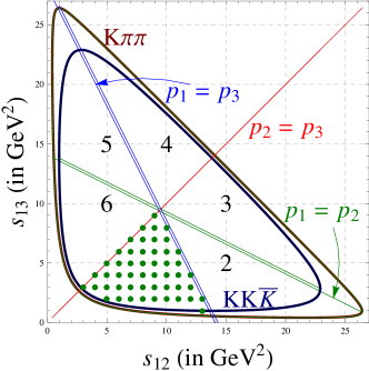
Figure 1: Kinematic boundaries and symmetry axes of $B\to K\pi\pi$ and $B\to KK{\bar{K}}$ Dalitz plots. The symmetry axes divide each plot into six zones, five of which are marked 2-6. The fifty dots in the region of overlap of the first of six zones from all Dalitz plots are used for the $\gamma$ measurement.

At this point it is important to mention that, in the current numerical analysis, we do not include correlations among observables at different points of the Dalitz plot. They can, in principle, be strongly correlated since they are calculated from the same constructed amplitudes, and not derived directly from the data. These correlations may have an important effect on the errors of the final result. Note also that the choice of resolution of 1 GeV² is completely ad hoc. There is no formal justification for this and it can also have a big effect on the final error since the error of the average of the $N$ values of $\gamma$ extracted from $N$ points of the Dalitz plot naively scales as $1/\sqrt{N}$. A more rigorous analysis needs to be performed directly from the data in order to avoid these assumptions.

For each of the 50 points we perform a maximum-likelihood fit within three scenarios (in order to test flavor-SU(3) breaking), and then combine all likelihood distributions. In the first scenario (Fit 1), the mode $B^{+}\to K^{+}\pi^{+}\pi^{-}$ is excluded and full SU(3) is assumed by setting $|\alpha_{SU(3)}|=1$. In the second scenario (Fit 2), $|\alpha_{SU(3)}|$ is calculated using the ratio of $X$’s from the $B^{0}\to K^{+}K^{0}K^{-}$ and $B^{+}\to K^{+}\pi^{+}\pi^{-}$ modes, and is then used in the fit with the other modes. Finally, in the last scenario (Fit 3), $|\alpha_{SU(3)}|$ is left as a free parameter and all five decays are fit simultaneously. The combined $-2\Delta\ln{\rm L}(\gamma)$ distributions for these three analyses are presented in Fig. 2.

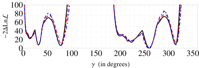
Figure 2: Results of the maximum-likelihood fits. The solid (black) curve represents the fit assuming flavor-SU(3) symmetry. The short dashes (red) represent the fit where flavor-SU(3) breaking is fixed by a point-by-point comparison of Dalitz plots for $B^{+}\to K^{+}\pi^{+}\pi^{-}$ and $B^{0}\to K^{+}K^{0}K^{-}$. The long dashes (blue) represent the fit with inputs from five Dalitz plots and an extra hadronic fit parameter $|\alpha_{SU(3)}|$.

All three scenarios produce very similar results, suggesting a small SU(3) breaking. There are four favored solutions, and this discrete ambiguity cannot be resolved without additional outside input. As an example, the numerical results of $\gamma$ for Fit 1 are $(31^{+2}_{-1})^{\circ}$, $(77\pm 2)^{\circ}$, $(261^{+2}_{-3})^{\circ}$ and $(314\pm 2)^{\circ}$. It is interesting to note that only one solution ($77^{\circ}$) is consistent with established direct measurements of $\gamma$. Let us emphasize again that the small error bars obtained are a consequence of the choice of the 1 GeV² grid, the fact that systematic effects are not included in the input numbers, and the fact that we do not include correlations among observables at different points of the Dalitz plots. These numbers are pedagogical examples containing several assumptions, but they are still values of $\gamma$ extracted from data of three-body $B$ decays. This proves that such an extraction can be done. This is the main point of this talk.

Finally, it is interesting to mention that the SU(3)-breaking parameter $|\alpha_{SU(3)}|$ can be extracted for each point of the Dalitz plot from the $A$’s and $\bar{A}$’s independently. Averaging over the 50 points, we find $|\alpha_{SU(3)}|=0.97\pm 0.04$ ($A$’s) or $0.99\pm 0.04$ ($\bar{A}$’s). These are consistent with one another and are also consistent with unity, again pointing towards a small SU(3)-breaking effect. The bottom line is that, even if SU(3) breaking is not under full control with the addition of a single breaking parameter, all clues suggest a small effect.

4 Conclusion

In this talk, we have described a new method for extracting the angle $\gamma$ from the data of $B\to K\pi\pi$ and $B\to KK{\bar{K}}$ decays, and we have demonstrated numerically that such an extraction can be done. All numbers presented here contain several simplifying assumptions, so that they should be regarded mostly as a pedagogical example. At present, it is impossible to predict what would be the output of a reproduction of this analysis performed directly from the data and including all statistical and correlation effects. But the fact is that three-body $B$ decays can provide additional constraints on $\gamma$.

- [1] B. Bhattacharya, M. Imbeault and D. London, Direct measurement of using and decays, hep-ph/1303.0846; B. Bhattacharya, M. Imbeault and D. London, Extraction of from three-body B decays, hep-ph/1212.1167; B. Bhattacharya, D. London and M. Imbeault, Measurement of gamma using B -¿ K pi pi and B -¿ K K Kbar decays, hep-ph/1306.5574.
- [2] N. R. -L. Lorier, M. Imbeault and D. London, Diagrammatic Analysis of Charmless Three-Body B Decays, Phys. Rev. D 84, 034040 (2011) [hep-ph/1011.4972].
- [3] M. Imbeault, N. R. -L. Lorier and D. London, Measuring in Decays, Phys. Rev. D 84, 034041 (2011) [hep-ph/1011.4973].
- [4] N. Rey-Le Lorier and D. London, Measuring with and Decays, Phys. Rev. D 85, 016010 (2012) [hep-ph/1109.0881].
- [5] J. P. Lees et al. [BABAR Collaboration], Amplitude Analysis of and Evidence of Direct CP Violation in decays, Phys. Rev. D 83, 112010 (2011) [hep-ex/1105.0125];
- [6] B. Aubert et al. [BABAR Collaboration], Time-dependent amplitude analysis of B0 —¿ K0(S) pi+ pi-, Phys. Rev. D 80, 112001 (2009) [hep-ex/0905.3615];
- [7] B. Aubert et al. [BABAR Collaboration], Evidence for Direct CP Violation from Dalitz-plot analysis of , Phys. Rev. D 78, 012004 (2008) [hep-ex/0803.4451];
- [8] J. P. Lees et al. [BABAR Collaboration], Study of CP violation in Dalitz-plot analyses of B0 —¿ K+K-K0(S), B+ —¿ K+K-K+, and B+ —¿ K0(S)K0(S)K+, Phys. Rev. D 85, 112010 (2012) [hep-ex/1201.5897];
- [9] J. P. Lees et al. [BABAR Collaboration], Amplitude analysis and measurement of the time-dependent CP asymmetry of decays, Phys. Rev. D 85, 054023 (2012) [hep-ex/1111.3636].