Distributed $n$-player approachability and consensus
in coalitional games

Abstract

We study a distributed allocation process where, repeatedly in time, every player renegotiates past allocations with neighbors and allocates new revenues. The average allocations evolve according to a doubly (over time and space) averaging algorithm. We study conditions under which the average allocations reach consensus to any point within a predefined target set even in the presence of adversarial disturbances. Motivations arise in the context of coalitional games with transferable utilities (TU) where the target set is any set of allocations that make the grand coalitions stable.

I Introduction

We consider a two-step distributed allocation process where at every time players first renegotiate their past allocations and second generate a new revenue and allocate it. The time-averaged allocations evolve according to a doubly (over time and space) averaging dynamics. The goal is to let all allocations reach consensus to any value in a predefined set even in the presence of an adversarial disturbance.

Motivations. The problem arises in the context of dynamic coalitional games with Transferable Utilities (TU games) [8]. A coalitional TU game consists in a set of players, who can form coalitions, and a characteristic function that provides a value for each coalition. The predefined set introduced above can be thought of as (but it is not limited to) the core of the game. This is the set of imputations under which no coalition has a value greater than the sum of its members’ payoffs. Therefore, no coalition has incentive to leave the grand coalition and receive a larger payoff.

Highlights of contributions. We analyze conditions under which the average allocations: (i) approach the set $X$ (Theorem 1), (ii) reach consensus, in which case we also compute the consensus value (Theorem 2), and (iii) are robust against disturbances (Theorem 3).

Related literature. Coalitional games with transferable utilities (TU) were first introduced by von Neumann and Morgenstern [14]. Here, a main issue is to study whether the core is an “approachable” set, and which allocation processes can drive the “complaint vector” to that set. Approachability theory was developed by Blackwell in the early ’56, [2], and is captured in the well known Blackwell’s Theorem. The geometric (approachability) principle that lies behind the Blackwell’s Theorem is among the fundamentals in allocation processes in coalitional games [7]. The discrete-time dynamics analyzed in the paper follows the rules of a typical consensus dynamics (see, e.g., [11] and references therein). among multiple agents, where an underlying communication graph for the agents and balancing weights have been used with some variations to reach an agreement on common decision variable in [10, 9, 11, 13, 12, 4] for distributed multi-agent optimization.

The paper is organized as follows. In Section, II, we formulate the problem and discuss motivations and main assumptions. In Section III, we illustrate the main results. In Section IV we provide numerical illustrations. Finally, in Section V, we provide concluding remarks and future directions.

Notation. We view vectors as columns. For a vector $x$, we use $[x]_{j}$ to denote its $j$th coordinate component. We let $x^{\prime}$ denote the transpose of a vector $x$, and $\|x\|$ denote its Euclidean norm. An $n\times n$ matrix $A$ is row-stochastic if the matrix has nonnegative entries $a^{i}_{j}$ and $\sum_{j=1}^{n}a^{i}_{j}=1$ for all $i=1,\ldots,n$. For a matrix $A$, we use $a^{i}_{j}$ or $[A]_{ij}$ to denote its $ij$th entry. A matrix $A$ is doubly stochastic if both $A$ and its transpose $A^{\prime}$ are row-stochastic. Given two sets $U$ and $S$, we write $U\subset S$ to denote that $U$ is a proper subset of $S$. We use $|S|$ for the cardinality of a given finite set $S$. We write $P_{X}[x]$ to denote the projection of a vector $x$ on a set $X$, and we write ${\rm dist}(x,X)$ for the distance from $x$ to $X$, i.e., $P_{X}[x]=\arg\min_{y\in X}\|x-y\|$ and ${\rm dist}(x,X)=\|x-P_{X}[x]\|$, respectively. Given a function of time $x(\cdot):\mathbb{N}\rightarrow\mathbb{R}$, we denote by $\bar{x}(t)$ its average up to time $t$, i.e., $\bar{x}(t):=\frac{1}{t}\sum_{\tau=1}^{t}x(\tau)$.

II Distributed reward allocation algorithm

Every player in a set $N=\{1,\ldots,n\}$ is characterized by an average allocation vector $\hat{x}_{i}(t+1)\in\mathbb{R}^{n}$. At every time he renegotiates with neighbors all past allocations and generates a new allocation vector $x_{i}(t+1)$. The time-averaged allocation $\hat{x}_{i}(t)$ evolves as follows:

$$\hat{x}_{i}(t+1)=\frac{t}{t+1}\left[\sum_{j=1}^{n}a^{i}_{j}(t)\hat{x}_{j}(t)\right]+\frac{1}{t+1}x_{i}(t+1),$$ (1)

where $a^{i}=(a^{i}_{1},\ldots,a^{i}_{n})^{\prime}$ is a vector of nonnegative weights consistent with the sparsity of the communication graph $\mathcal{G}(t)=(N,\mathcal{E}(t))$. A link $(j,i)\in\mathcal{E}(t)$ exists if player $j$ is a neighbor of player $i$ at time $t$, i.e. if player $i$ renegotiates allocations with player $j$ at time $t$.

Problem. Our goal is to study under what conditions all allocation vectors converge to a unique value and this value belongs to a predefined set $X$: for all $i,j\in V$,

$$\hat{x}_{i}(t)=\hat{x}_{j}(t)\in X,\quad\mbox{for $t\rightarrow\infty$}.$$ (2)

In the sequel, we rewrite equation (1) in the compact form:

$$\hat{x}_{i}(t+1)=\frac{t}{t+1}w_{i}(t)+\frac{1}{t+1}x_{i}(t+1),$$ (3)

where $w_{i}(t)$ is the space average defined as

$$w_{i}(t)=\left[\sum_{j=1}^{n}a^{i}_{j}(t)\hat{x}_{j}(t)\right].$$ (4)

II-A Motivations

The set $X$ introduced above can be thought of as the core of a coalitional game with Transferable Utilities (TU game).

A coalitional TU game is defined by a pair $<N,\eta>$, where $N=\{1,\ldots,n\}$ is a set of players and $\eta:2^{N}\rightarrow{\mathbb{R}}$ a function defined for each coalition $S\subseteq N$ ($S\in 2^{N}$). The function $\eta$ determines the value $\eta(S)$ assigned to each coalition $S\subset N$, with $\eta(\emptyset)=0$. We let $\eta_{S}$ be the value $\eta(S)$ of the characteristic function $\eta$ associated with a nonempty coalition $S\subseteq N$. Given a TU game $<N,\eta>$, let $C(\eta)$ be the core of the game,

$$\begin{split}C(\eta)&=\left\{x\in\mathbb{R}^{n}\,\Big{|}\,\sum_{j\in N}[x]_{j}=\eta_{N},\ \right.\\ &\qquad\left.\sum_{j\in S}[x]_{j}\geq\eta_{S}\hbox{ for all nonempty }S\subset N\right\}.\end{split}$$

Essentially, the core of the game is the set of all allocations that make the grand coalition stable with respect to all subcoalitions. Condition $\sum_{j\in N}[x]_{j}=\eta_{N}$ is also called efficiency condition. Condition $\sum_{j\in S}[x]_{j}\geq\eta_{S}$ for all nonempty $S\subset N$ is referred to as “stability with respect to subcoalitions”, since it guarantees that the total amount given to the members of a coalition exceeds the value of the coalition itself.

II-B Main assumptions

Following [11] (see also [8]) we can make the following assumptions on the information structure. We let $A(t)$ be the weight matrix with entries $a^{i}_{j}(t)$.

Assumption 1

Each matrix $A(t)$ is doubly stochastic with positive diagonal. Furthermore, there exists a scalar $\alpha>0$ such that $a^{i}_{j}(t)\geq\alpha$ whenever $a^{i}_{j}(t)>0$.

At any time, the instantaneous graph $\mathcal{G}(t)$ need not be connected. However, for the proper behavior of the process, the union of the graphs $\mathcal{G}(t)$ over a period of time is assumed to be connected.

Assumption 2

There exists an integer $Q\geq 1$ such that the graph $\left(N,\bigcup_{\tau=tQ}^{(t+1)Q-1}\mathcal{E}(\tau)\right)$ is strongly connected for every $t\geq 0$.

It is worth noting that the above assumptions are fairly standard in the distributed computation literature. In particular, the joint strong connectivity is the weakest possible assumption to guarantee persistent circulation of the information through the graph. The double stochasticity of the matrix $A(t)$ is a common assumption to guarantee average consensus.

Let $X\subset\mathbb{R}^{n}$ be the core set of the game. A common assumption in approachability theory is that both the core set is convex and bounded, and the payoff (or loss) vectors generated at each time are bounded. Thus, following [2, 5], we borrow and adapt such an assumption to our framework.

Assumption 3

The core set $X$ is nonempty.

Notice that a nonempty core is a convex and compact set.

The next assumption indicates how the new reward vector has to be generated in order to obtain approachability.

Assumption 4

For each $i\in N$ the new reward vector $x_{i}(\cdot)$ is bounded, i.e., there exists $L>0$ s.t. $\forall t\geq 0\;\|x_{i}(t+1)\|\leq L$, and satisfies the following inequality, for a scalar negative number, $\phi<0$,

$$\left(w_{i}(t)-P_{X}(w_{i}(t))\right)^{\prime}\left(x_{i}(t+1)-P_{X}(w_{i}(t)\right)\leq\phi<0.$$

From a geometric standpoint, Assumption 4 requires that, given the two half-spaces identified by the supporting hyperplane of $X$ through $P_{X}(w_{i}(t))$, the new reward vector $x_{i}(t+1)$ lies in the half-space not containing $w_{i}(t)$.

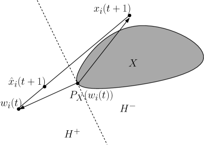
Figure 1: Approachability principle.

III Main results

Next, we provide the main results of the paper. Namely, we prove that the average allocations: (i) approach the set $X$ (Theorem 1), (ii) reach consensus (Theorem 2), and (iii) are robust against disturbances (Theorem 3).

III-A Approachability and consensus

Before stating the first theorem, we need to introduce two lemmas. The next lemma establishes that the space averaging step in (1) reduces the total distance (i.e. the sum of distances) of the estimates from the set $X$.

Lemma 1

Let Assumption 1 hold. Then the total distance from $X$ decreases when replacing the allocations $\hat{x}_{i}(t)$ by their space averages $w_{i}(t)$, i.e.,

$$\sum_{i=1}^{n}{\rm dist}(w_{i}(t),X)\leq\sum_{i=1}^{n}{\rm dist}(\hat{x}_{i}(t),X).$$

As a preliminary step to the next result, observe that, from the definition of ${\rm dist}(\cdot,X)$ and from (1) and (4), it holds

$$\begin{split}{\rm dist}&(\hat{x}_{i}(t+1),X)^{2}=\|\hat{x}_{i}(t+1)-P_{X}[\hat{x}_{i}(t+1)]\|^{2}\\ &\leq\|\hat{x}_{i}(t+1)-P_{X}[w_{i}(t)]\|^{2}\\ &=\left\|\frac{t}{t+1}w_{i}(t)+\frac{1}{t+1}x_{i}(t+1)-P_{X}[w_{i}(t)]\right\|^{2}\\ &=\left\|\frac{t}{t+1}\left(w_{i}(t)-P_{X}[w_{i}(t)]\right)\right.\\ &\qquad\left.+\frac{1}{t+1}\left(x_{i}(t+1)-P_{X}[w_{i}(t)]\right)\right\|^{2}\\ &=\left(\frac{t}{t+1}\right)^{2}\|w_{i}(t)-P_{X}[w_{i}(t)]\|^{2}\\ &\qquad+\left(\frac{1}{t+1}\right)^{2}\|x_{i}(t+1)-P_{X}[w_{i}(t)]\|^{2}\\ &+\frac{2t}{(t+1)^{2}}(w_{i}(t)-P_{X}[w_{i}(t)])^{\prime}(x_{i}(t+1)-P_{X}[w_{i}(t)]).\end{split}$$ (5)

The following lemma states that, under the approachability assumption, the distance of each single estimate from $X$ decreases with respect to the one of the spatial average when applying the time averaging step.

Lemma 2

Let Assumptions 3-4 hold. Then, there exists a positive integer scalar, $\tilde{t}>0$, such that for all $t\geq\tilde{t}>0$ the distance of each single $\hat{x}_{i}(t+1)$ decreases in comparison with the distance of $w_{i}(t)$, i.e.,

$${\rm dist}(\hat{x}_{i}(t+1),X)<{\rm dist}(w_{i}(t),X),\quad\forall i=1,\ldots,n$$

We are now ready to state the first main result.

Theorem 1

Let Assumptions 1-4 hold. Then all average allocations approach set $X$, i.e.,

$$\lim_{t\rightarrow\infty}\sum_{i=1}^{n}{\rm dist}(\hat{x}_{i}(t),X)=0.$$

Next, let us introduce the barycenter of respectively the estimates and the reward vectors

$$\hat{x}_{b}(t):=\frac{1}{n}\sum_{i=1}^{n}\hat{x}_{i}(t)\qquad\text{and}\qquad x_{b}(t):=\frac{1}{n}\sum_{i=1}^{n}x_{i}(t).$$

Consistently, let us denote as $\bar{x}_{b}(t)$ the time average of the barycenter, i.e.

$$\bar{x}_{b}(t)=\frac{1}{t+1}\sum_{\tau=0}^{t}x_{b}(\tau).$$

The following lemma establishes that the barycenter of the estimates evolves as the time average $\bar{x}_{b}(t)$ of the barycenter of the reward vectors generated by the players.

Lemma 3

The barycenter of the local allocations $\hat{x}_{b}(t)$ coincides at each time $t$ with the time-average of the barycenter of the generated reward vectors $\bar{x}_{b}(t)$.

The following theorem establishes that all allocations converge to $\bar{x}_{b}(t)$, which in the limit must belong to $X$ according to Theorem 1.

Theorem 2

(Consensus to the barycenter time-average) Let Assumptions 1-4 hold. Then, all players reach consensus on the time-average of the barycenter of the reward vectors generated by each player, $\bar{x}_{b}(t)$, i.e.,

$$\lim_{t\rightarrow\infty}\|\hat{x}_{i}(t)-\bar{x}_{b}(t)\|=0\quad\forall i=1,\ldots,n.$$

Summarizing the two main results, we have proven that asymptotically all the players’ allocations converge to the time-average of the barycenter of the generated reward vectors and that this vector lies in the core of the game.

III-B Adversarial disturbance

Here we analyze the case where, for each player $i\in N$, the input $x_{i}(\cdot)$ is the payoff of a repeated two-player game between player $i$ (Player $i_{1}$) and an (external) adversary (Player $i_{2}$). With some slight abuse of notation we denote $S_{1}$ and $S_{2}$ the finite set of actions of players $i_{1}$ and $i_{2}$ respectively.

The instantaneous payoff $x_{i}(t)$ at time $t$ is given by a function $\phi_{i}:S_{1}\times S_{2}\to\mathbb{R}^{n}$ as follows:

$$x_{i}(t)=\phi(j(t),k(t)),$$

where $j(t)\in S_{1}$ and $k(t)\in S_{2}$. We extend $x_{i}$ to the set of mixed actions pairs, $\Delta(S_{1})\times\Delta(S_{2})$, in a bilinear fashion. In particular, for every pair of mixed strategies $(p(t),q(t))\in\Delta(S_{1})\times\Delta(S_{2})$ for player $i_{1}$ and $i_{2}$ at time $t$, the expected payoff is

$$\mathbb{E}x_{i}(t)=\sum_{j\in S_{1}}\sum_{k\in S_{2}}p_{j}(t)q_{k}(t)\phi(j,k).$$

For simplicity the one-shot vector-payoff game $(S_{1},S_{2},x_{i})$ is denoted by $G_{i}$.

Let $\lambda\in\mathbb{R}^{n}$. Denote by $\langle\lambda,G_{i}\rangle$ the zero-sum one-shot game whose set of players and their action sets are as in the game $G_{i}$, and the payoff that player 2 pays to player 1 is $\lambda^{\prime}\phi(j,k)$ for every $(j,k)\in S_{1}\times S_{2}$.

The resulting zero-sum game is described by the matrix

$$\Phi_{\lambda}=[\lambda^{\prime}\phi(j,k)]_{j\in S_{1},k\in S_{2}}.$$

As a zero-sum one-shot game, the game $\langle\lambda,G_{i}\rangle$ has a value, denoted

$$v_{\lambda}:=\min_{p\in\Delta S_{1}}\max_{q\in\Delta S_{2}}p^{\prime}\Phi_{\lambda}q=\max_{q\in\Delta S_{2}}\min_{p\in\Delta S_{1}}p^{\prime}\Phi_{\lambda}q.$$

For every mixed action $p\in\Delta(S_{1})$ denote $D_{1}(p)$ the set of all payoffs that might be realized when player $i_{1}$ plays the mixed action $p$:

$$D_{1}(p)=\{x_{i}(p,q)\colon q\in\Delta(S_{2})\}.$$

If $v_{\lambda}\geq 0$ (resp. $v_{\lambda}>0$), then there is a mixed action $p\in\Delta(S_{1})$ such that $D_{1}(p)$ is a subset of the closed half space $\{x\in\mathbb{R}^{n}\colon\lambda^{\prime}x\geq 0\}$ (resp. half space $\{x\in\mathbb{R}^{m}\colon\lambda^{\prime}x>0\}$).

Let us introduce next the counterpart of Assumption 4 in this new worst-case setting.

Assumption 5

For any $w_{i}(t)\in\mathbb{R}^{n}$, there exists a mixed strategy $p(t+1)\in\Delta(S_{1})$ for Player $i_{1}$ such that, for all mixed strategy $q(t+1)\in\Delta(S_{2})$ of Player $i_{2}$, the new reward vector $x_{i}(\cdot)$ is bounded, i.e. there exists $L>0$ s.t. $\forall t\geq 0\;\|x_{i}(t+1)\|\leq L$, and satisfies

$$\left(w_{i}(t)-P_{X}(w_{i}(t))\right)^{\prime}\left(\mathbb{E}x_{i}(t+1)-P_{X}(w_{i}(t)\right)\leq\phi<0,$$

where $\mathbb{E}x_{i}(t+1)=\sum_{j\in S_{1}}\sum_{k\in S_{2}}p_{j}(t+1)q_{k}(t+1)\phi(j,k).$

The above condition is among the foundations of approachability theory as it guarantees that the average payoff $\frac{1}{T}\sum_{t=0}^{T-1}x_{i}(t)$ converges almost surely to $X$ (see, e.g., [2] and also [5], chapter 7). Here we adapt the above condition to the multi-agent and distributed scenario under study.

Corollary III.1 (see [2], Corollary 2)

Any convex set $X\subset\mathbb{R}^{n}$ is approachable if and only if $v_{\lambda}<0$ for any $\lambda\in\mathbb{R}^{n}$.

Next we show that if the approachability condition expressed above holds true, then $dist(\hat{x}_{i},X)$ tends to zero for any $X$. We write $w.p.1$ to mean “with probability 1”.

Theorem 3

Let Assumptions 1-3 and 5 hold. Then all average allocations approach set $X$, i.e.,

$$\lim_{t\rightarrow\infty}\sum_{i=1}^{n}{\rm dist}(\hat{x}_{i}(t),X)=0,\quad w.p.1.$$

We conclude this section by observing that Theorem 2 still holds and therefore all players’ estimates reach consensus on the time-average of the barycenter of the reward vectors generated by each player.

IV Simulations

We illustrate the results in a game with four players, $N=\{1,\ldots,4\}$, communicating according to a fixed undirected cycle graph. That is, $\mathcal{G}(t)=(N,\mathcal{E})$ where $\mathcal{E}=\{(i,j)\;|\;j=i+1,i\in\{1,\ldots n-1\}\;\text{or}\;(i,j)=(n,1)\}$.

We set $\eta_{\{1\}}=\ldots=\eta_{\{4\}}=2$, $\eta_{\{1,2\}}=5$, $\eta_{\{3,4\}}=5$, $\eta_{\{1,2,3\}}=7$ and $\eta_{N}=10$ ($\eta_{S}$ is the value of coalition $S$). That is, each player expects to receive at least a reward of $2$ which is its value as a singleton coalition. But, for example, players $1$ and $2$ expect to be more valuable if they form a coalition as well as $3$ and $4$. Consistently, the core of the game is the polyhedral set given by

$$\begin{split}C(\eta)=\Big{\{}x\in\mathbb{R}^{4}\,\Big{|}\,x_{1}+x_{2}+x_{3}+x_{4}=10,\\ x_{1}+x_{2}+x_{3}\geq 7,\ x_{1}+x_{2}\geq 5,\\ \ x_{3}+x_{4}\geq 5,x_{1}\geq 2,\ldots,x_{4}\geq 2\Big{\}}.\end{split}$$

We initialize the assignments assuming each player assign itself the entire reward. That is, denoting $b_{i}\in{\mathbb{R}}^{n}$ the $i$-th canonical vector (so that, e.g., $b_{1}=[1\;0\;\ldots\;0]^{\prime}$), we set $\hat{x}_{i}(0)=10\,b_{i}$ for all $i\in\{1,\ldots,n\}$. At every iteration $t\in{\mathbb{N}}$, each player chooses the new reward vector $x_{i}(t+1)$ according to the approachability principle. In particular, we set $x_{i}(t+1)=P_{X}[w_{i}(t)]+\alpha\,(P_{X}[w_{i}(t)]-w_{i}(t))+v^{\top}$, where $\alpha$ is a random number uniformly distributed in $[0,1]$ and $v^{\top}$ a random vector belonging to the hyperplane tangent to the core at $P_{X}[w_{i}(t)]$ with coordinates uniformly chosen in $[0,1]$. The temporal evolution of the local estimates of the average reward vector is depicted in Figure 2. As expected the local estimates converge to the same average assignment which is the point of the core $[3.8\;\,3\;\,2.2\;\,1]^{\prime}$.

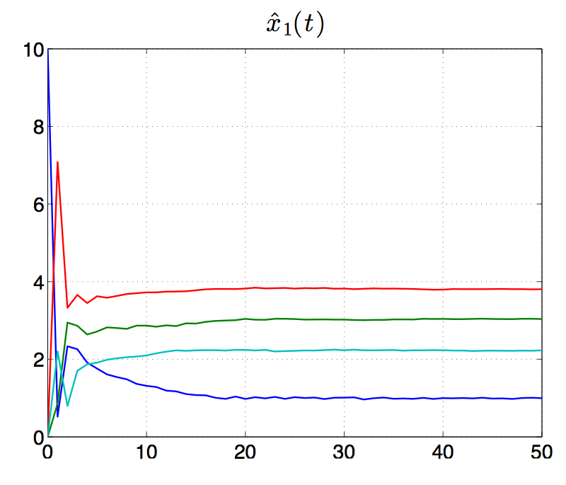
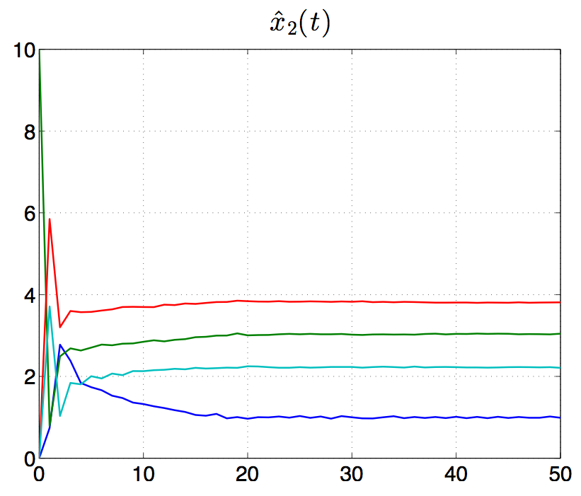
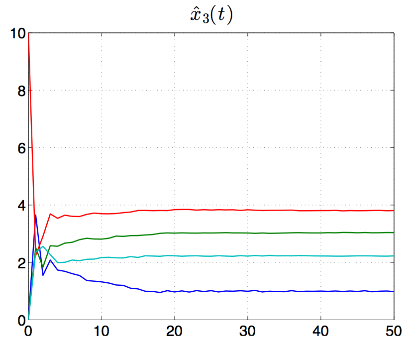
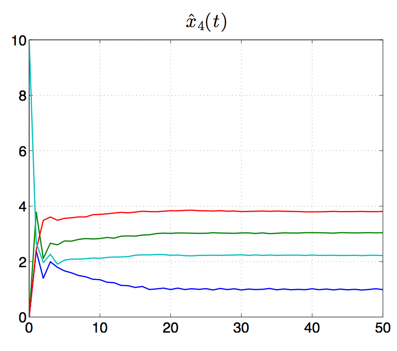
Figure 2: Local average reward vectors

V Conclusions

We have analyzed convergence conditions of a distributed allocation process arising in the context of TU games. Future directions include the extension of our results to population games with mean-field interactions, and averaging algorithms driven by Brownian motions.

Appendix

Proof of Lemma 1

By convexity of the distance function ${\rm dist}(\cdot,X)$ and from (4) we have

$${\rm dist}(w_{i}(t),X)\leq\sum_{j=1}^{n}a^{i}_{j}(t){\rm dist}(\hat{x}_{j}(t),X).$$

Summing over $i=1,\ldots,n$ both sides of the above inequality we obtain

$$\begin{split}&\sum_{i=1}^{n}{\rm dist}(w_{i}(t),X)\leq\sum_{i=1}^{n}\sum_{j=1}^{n}a^{i}_{j}(t){\rm dist}(\hat{x}_{j}(t),X)\\ =&\sum_{j=1}^{n}\left(\sum_{i=1}^{n}a^{i}_{j}(t)\right){\rm dist}(\hat{x}_{j}(t),X)=\sum_{j=1}^{n}{\rm dist}(\hat{x}_{j}(t),X),\\ \end{split}$$

where the last equality follows from the stochasticity of $A(t)$ in Assumption 1. This concludes the proof.

Proof of Lemma 2

Rearranging equation (5) we obtain

$$\begin{split}\|\hat{x}_{i}(t+1)-P_{X}[\hat{x}_{i}(t+1)]\|^{2}\\ -\frac{t^{2}}{(t+1)^{2}}\|w_{i}(t)-P_{X}[w_{i}(t)]\|^{2}\leq\\ \;\frac{1}{(t+1)^{2}}\|x_{i}(t+1)-P_{X}[w_{i}(t)]\|^{2}\\ +\frac{2t}{(t+1)^{2}}(w_{i}(t)-P_{X}[w_{i}(t)])^{\prime}(x_{i}(t+1)-P_{X}[w_{i}(t)]).\\ \end{split}$$ (6)

Note that the left hand side in (6) approximates ${\rm dist}(\hat{x}_{i}(t+1),X)^{2}-{\rm dist}(w_{i}(t),X)^{2}$ for increasing $t$ and also that for all $t$ the left hand side upper bounds such a difference, i.e.,

$$\begin{split}{\rm dist}(\hat{x}_{i}(t+1),X)^{2}-{\rm dist}(w_{i}(t),X)^{2}\\ \leq{\rm dist}(\hat{x}_{i}(t+1),X)^{2}-\frac{t^{2}}{(t+1)^{2}}{\rm dist}(w_{i}(t),X)^{2}\quad\forall t.\end{split}$$

It remains to note that there exists a great enough scalar integer $\tilde{t}$ such that the left hand side in (6) is negative for all $t\geq\tilde{t}$. From the boundedness of set $X$ and of vectors $x_{i}(t)$, there exists $M>0$ such that $\|x_{i}(t+1)-P_{X}[w_{i}(t)]\|^{2}<M$. Thus, we have

$$\begin{split}{\rm dist}(\hat{x}_{i}(t+1),X)^{2}-{\rm dist}(w_{i}(t),X)^{2}\\ \leq{\rm dist}(\hat{x}_{i}(t+1),X)^{2}-\frac{t^{2}}{(t+1)^{2}}{\rm dist}(w_{i}(t),X)^{2}\\ \leq\frac{1}{(t+1)^{2}}\big{(}\|x_{i}(t+1)-P_{X}[w_{i}(t)]\|^{2}\\ +2t(w_{i}(t)-P_{X}[w_{i}(t)])^{\prime}(x_{i}(t+1)-P_{X}[w_{i}(t)])\big{)}\\ \leq\frac{1}{(t+1)^{2}}(M+2t\phi)<0\end{split}$$ (7)

Taking $\tilde{t}>-M/2\phi>0$ concludes the proof.

Proof of Theorem 1

Recall from (5) that

$$\begin{split}\|\hat{x}_{i}(t+1)-P_{X}[\hat{x}_{i}(t+1)]\|^{2}\leq\\ \left(\frac{t}{t+1}\right)^{2}\|w_{i}(t)-P_{X}[w_{i}(t)]\|^{2}\\ +\left(\frac{1}{t+1}\right)^{2}\|x_{i}(t+1)-P_{X}[w_{i}(t)]\|^{2}\\ \;+2\frac{t}{(t+1)^{2}}(w_{i}(t)-P_{X}[w_{i}(t)])^{\prime}(x_{i}(t+1)-P_{X}[w_{i}(t)]).\end{split}$$

From Lemma 1 and rearranging the above inequality, we have

$$\begin{split}\sum_{i=1}^{n}\big{[}(t+1)^{2}\|\hat{x}_{i}(t+1)-P_{X}[\hat{x}_{i}(t+1)]\|^{2}\\ -t^{2}\|\hat{x}_{i}(t)-P_{X}[\hat{x}_{i}(t)]\|^{2}\big{]}\\[5.16663pt] \leq\sum_{i=1}^{n}\Big{[}\|x_{i}(t+1)-P_{X}[w_{i}(t)]\|^{2}\\ +2t(w_{i}(t)-P_{X}[w_{i}(t)])^{\prime}(x_{i}(t+1)-P_{X}[w_{i}(t)])\Big{]}\\[5.16663pt] \leq\sum_{i=1}^{n}\left[\|x_{i}(t+1)-P_{X}[w_{i}(t)]\|^{2}\right.,\end{split}$$

where the last inequality is due to Assumption 4. Summing over $t=0,\ldots,\tau-1$, and noting that $\|x_{i}(t+1)-P_{X}[w_{i}(t)]\|$ is bounded (from Assumption 3), so that the right hand side is upper bounded by some $M>0$, we obtain

$$\sum_{i=1}^{n}\tau^{2}\|\hat{x}_{i}(\tau)-P_{X}[\hat{x}_{i}(\tau)]\|^{2}\leq M\tau$$

from which $\|\hat{x}_{i}(\tau)-P_{X}[\hat{x}_{i}(\tau)]\|^{2}\leq\frac{M}{\tau}$, and therefore $\lim_{\tau\rightarrow\infty}\|\hat{x}_{i}(\tau)-P_{X}[\hat{x}_{i}(\tau)]\|^{2}=0$, which concludes the proof.

Proof of Lemma 3

To prove the statement observe that $\bar{x}_{b}(0)=\hat{x}_{b}(0)=x_{b}(0)$. Thus, we prove that $\bar{x}_{b}(t)$ and $\hat{x}_{b}(t)$ satisfy the same dynamics. By definition of time-average, $\bar{x}_{b}(t)$ satisfies the dynamics

$$\bar{x}_{b}(t+1)=\frac{t}{t+1}\bar{x}_{b}(t)+\frac{1}{t+1}x_{b}(t+1).$$ (8)

The dynamics of $\hat{x}_{b}(t)$ is

$$\frac{1}{n}\sum_{i=1}^{n}\hat{x}_{i}(t+1)=\frac{1}{n}\Big{[}\frac{t}{t+1}\sum_{i=1}^{n}\sum_{j=1}^{n}a^{i}_{j}(t)\hat{x}_{j}(t)$$

$$+\frac{1}{t+1}\sum_{i=1}^{n}x_{i}(t+1)\Big{]}.$$

Exchanging the sum signs

$$\hat{x}_{b}(t+1)=\frac{1}{n}\frac{t}{t+1}\sum_{j=1}^{n}\sum_{i=1}^{n}a^{i}_{j}(t)\hat{x}_{j}(t)+\frac{1}{t+1}x_{b}(t+1),$$

and, by Assumption 1 ($A(t)$ is doubly stochastic),

$$\begin{split}\hat{x}_{b}(t+1)=\frac{1}{n}\frac{t}{t+1}\sum_{j=1}^{n}\hat{x}_{j}(t)+\frac{1}{t+1}x_{b}(t+1)\\ =\frac{t}{t+1}\hat{x}_{b}(t)+\frac{1}{t+1}x_{b}(t+1),\end{split}$$

which is the same dynamics as (8), thus concluding the proof.

Proof of Theorem 2

Using the previous lemma we can show that $\hat{x}_{i}(t)$ converges to $\hat{x}_{b}(t)$. Let us introduce the error of the estimate $\hat{x}_{i}(t)$ from the barycenter, i.e. $\hat{e}_{i}(t)=\hat{x}_{i}(t)-\hat{x}_{b}(t)$. The error dynamics is given by

$$\begin{split}\hat{e}_{i}(t+1)=\frac{t}{t+1}\left[\sum_{j=1}^{n}a^{i}_{j}(t)\hat{e}_{j}(t)+\sum_{j=1}^{n}a_{j}^{i}\hat{x}_{b}(t)\right]\\ +\frac{1}{t+1}e_{i}(t+1)+\frac{1}{t+1}x_{b}(t+1)\\[5.16663pt] -\frac{t}{t+1}\hat{x}_{b}(t)-\frac{1}{t+1}x_{b}(t+1),\end{split}$$

where $e_{i}(t)=x_{i}(t)-x_{b}(t)$. Thus

$$\hat{e}_{i}(t+1)=\frac{t}{t+1}\big{(}\sum_{j=1}^{n}a^{i}_{j}(t)\hat{e}_{j}(t)\big{)}+\frac{1}{t+1}e_{i}(t+1).$$

Multiplying both sides by $(t+1)$ and taking $t$ inside the sum,

$$(t+1)\hat{e}_{i}(t+1)=\sum_{j=1}^{n}a^{i}_{j}(t)t\hat{e}_{j}(t)+e_{i}(t+1).$$

Defining $\hat{z}_{i}(t)=t\,\hat{e}_{i}(t)$, we have

$$\hat{z}_{i}(t+1)=\sum_{j=1}^{n}a^{i}_{j}(t)\hat{z}_{j}(t)+e_{i}(t+1).$$

In vector form the above equation turns to be

$$\hat{z}(t+1)=\big{(}A(t)\otimes I_{n}\big{)}\hat{z}(t)+e(t+1),$$ (9)

with $\hat{z}(t)=[z_{1}(t)\;\ldots\;z_{n}(t)]^{\prime}$, $\hat{e}(t)=[e_{1}(t)\;\ldots\;e_{n}(t)]^{\prime}$, $I_{n}$ the identity matrix of dimension $n$ and $\otimes$ the Kronecker product. Notice that denoting $[\hat{z}]_{\ell}=\big{[}[\hat{z}_{1}]_{\ell}\;\ldots\;[\hat{z}_{n}]_{\ell}\big{]}$ and $[e]_{\ell}=\big{[}[e_{1}]_{\ell}\;\ldots\;[e_{n}]_{\ell}\big{]}$, $\ell\in\{1,\ldots,n\}$, the dynamics of each $[\hat{z}]_{\ell}$ is given by

$$[\hat{z}]_{\ell}(t+1)=A(t)[\hat{z}]_{\ell}(t)+[e]_{\ell}(t+1).$$ (10)

Thus, we can simply work on each component separately. Slightly abusing notation we neglect the subscript of $[\hat{z}]_{\ell}$ and $[e]_{\ell}$, and write $\hat{z}(t)$ and $e(t)$.

It is worth noting that the driven system (10), and so (9), is not bounded-input-bounded-state stable (when a general input signal is allowed). That is, for general initial condition and input signal the state trajectory may diverge. We show that for the special initial condition ($\hat{z}(t)=0$ by construction) and class of input signals ($\mathbf{1}^{\prime}e(t+1)=0$ by definition) under consideration, the state trajectories of (9) are bounded.

First, let us observe that, multiplying both sides of (9) by the vector $\mathbf{1}^{\prime}=[1\;\ldots\;1]$, we get

$$\begin{split}\mathbf{1}^{\prime}\hat{z}(t+1)&=\mathbf{1}^{\prime}A(t)\hat{z}(t)+\mathbf{1}^{\prime}e(t+1)\\ &=\mathbf{1}^{\prime}\hat{z}(t).\end{split}$$ (11)

Since $\hat{z}(0)=0$ by construction, it holds $\mathbf{1}^{\prime}\hat{z}(t)=0$ for all $t\in{\mathbb{N}}$. That is, $\hat{z}(t)$ is orthogonal to the vector $\mathbf{1}$ for all $t$.

Next, we show that the trajectory $\hat{z}(\cdot)$ is bounded. Following [3], let $P\in{\mathbb{R}}^{(n-1)\times n}$ be a matrix defining an orthogonal projection onto the space orthogonal to span{$\mathbf{1}$}. It holds that $P\mathbf{1}=0$ and $\|Px\|_{2}=\|x\|_{2}$ if $x^{\prime}\mathbf{1}=0$. Thus, from equation (11) we have that $\|P\hat{z}(t)\|_{2}=\|\hat{z}(t)\|_{2}$ for all $t$. Therefore, proving boundedness of $\hat{z}(\cdot)$ is equivalent to showing that $P\hat{z}(\cdot)$ is bounded. For a given $P$, associated to any $A(t)$ satisfying Assumption 1, there exists $\bar{A}(t)$ satisfying $PA(t)=\bar{A}(t)P$. The spectrum of $\bar{A}(t)$ is the spectrum of $A(t)$ after removing the eigenvalue $1$. Multiplying both sides of equation (9) by $P$, we get

$$\begin{split}P\hat{z}(t+1)&=PA(t)\hat{z}(t)+Pe(t+1)\\ &=\bar{A}(t)P\hat{z}(t)+Pe(t+1).\end{split}$$ (12)

Under Assumptions 1 and 2, the undriven dynamics $y(t+1)=\bar{A}(t)y(t)$ is uniformly exponentially stable, i.e., $||y(t)||<C\rho^{t}||y(0)||$ with $C$ and $\rho<1$ independent of $y(0)$ and depending only on $n$, $Q$ and $\alpha$ (see Theorem 9.2 and Corollary 9.1 in [6]). Thus, the state trajectories of (12) are bounded for any bounded signal $Pe(t+1)$ with $\mathbf{1}^{\prime}e(t)=0$. Since $\mathbf{1}^{\prime}e(t)=0$ for all $t$, we have $\|Pe(t)\|_{2}=\|e(t)\|_{2}$ for all $t$, which is bounded. The proof follows by recalling that $\|P\hat{z}(t)\|_{2}=\|\hat{z}(t)\|_{2}$ and that $\hat{z}(t)=t\hat{e}(t)$.

Proof of Theorem 3

From (5), invoking Lemma 1 and using Assumption 5 we have

$$\begin{split}\sum_{i=1}^{n}\big{[}(t+1)^{2}\|\hat{x}_{i}(t+1)-P_{X}[\hat{x}_{i}(t+1)]\|^{2}\\ -t^{2}\|\hat{x}_{i}(t)-P_{X}[\hat{x}_{i}(t)]\|^{2}\big{]}\\[5.16663pt] \leq\sum_{i=1}^{n}\Big{[}\|x_{i}(t+1)-P_{X}[w_{i}(t)]\|^{2}\\ +2t(w_{i}(t)-P_{X}[w_{i}(t)])^{\prime}(x_{i}(t+1)-\mathbb{E}x_{i}(t+1))\Big{]},\end{split}$$

Summing over $t=0,\ldots,\tau-1$, and noting that $\|x_{i}(t+1)-P_{X}[w_{i}(t)]\|$ is upper bounded (from Assumption 3) by some $M>0$, we obtain

$$\begin{split}\sum_{i=1}^{n}\|\hat{x}_{i}(\tau)-P_{X}[\hat{x}_{i}(\tau)]\|^{2}\\ \leq\frac{M}{\tau}+\frac{1}{\tau}\sum_{t=0}^{\tau-1}\sum_{i=1}^{n}K^{i}_{t}\|x_{i}(t+1)-\mathbb{E}x_{i}(t+1)\|\end{split}$$

where $K^{i}_{t}=\frac{1}{\tau}2t\|w_{i}(t)-P_{X}[w_{i}(t)]\|$. Now, using $\|x_{i}(t+1)\|\leq L\;\forall t\geq 0$ from Assumption 5 and from (3) and (4) we have that $w_{i}(t)$ is bounded which in turn implies that $\|w_{i}(t)-P_{X}[w_{i}(t)]\|$ is bounded. Then, the second term in the right-hand side is an average of bounded zero-mean martingale differences, and therefore the Hoeffding-Azuma inequality (together with the Borel-Cantelli lemma) immediately implies that

$$\lim_{\tau\rightarrow\infty}\sum_{i=0}^{n}\|\hat{x}_{i}(\tau)-P_{X}[\hat{x}_{i}(\tau)]\|^{2}=0$$

which concludes the proof.

References

- [1] D. Bauso and G. Notarstefano. Distributed -player approachability via time and space average consensus. In 3rd IFAC Workshop on Distributed Estimation and Control in Networked Systems, pages 198–203, Santa Barbara, CA, USA, Sept 2012.
- [2] D. Blackwell. An analog of the minmax theorem for vector payoffs. Pacific J. Math., 6:1–8, 1956.
- [3] Vincent D Blondel, Julien M Hendrickx, Alex Olshevsky, and John N Tsitsiklis. Convergence in multiagent coordination, consensus, and flocking. In 44th IEEE Conf. on Decision and Control, 2005, pages 2996–3000, 2005.
- [4] M. Bürger, G. Notarstefano, F. Allgöwer, and F. Bullo. A distributed simplex algorithm for degenerate linear programs and multi-agent assignments. Automatica, 48(9):2298–2304, Sept 2012.
- [5] N. Cesa-Bianchi and G. Lugosi. Prediction, Learning, and Games. Cambridge University Press, 2006.
- [6] Julien M Hendrickx. Graphs and networks for the analysis of autonomous agent systems. PhD thesis, Ecole Polytechnique, 2008.
- [7] E. Lehrer. Allocation processes in cooperative games. International J. of Game Theory, 31:341–351, 2002.
- [8] A. Nedić and D. Bauso. Dynamic coalitional tu games: Distributed bargaining among players’ neighbors. IEEE Trans. Autom. Control, 58(6):1363–1376, 2013.
- [9] A. Nedić, A. Olshevsky, A. Ozdaglar, and J.N. Tsitsiklis. On distributed averaging algorithms and quantization effects. IEEE Trans. Autom. Control, 54(11):2506–2517, 2009.
- [10] A. Nedić and A. Ozdaglar. Distributed subgradient methods for multi-agent optimization. IEEE Trans. Autom. Control, 54(1):48–61, 2009.
- [11] A. Nedić, A. Ozdaglar, and P.A. Parrilo. Constrained consensus and optimization in multi-agent networks. IEEE Trans. Autom. Control, 55(4):922–938, 2010.
- [12] G. Notarstefano and F. Bullo. Distributed abstract optimization via constraints consensus: Theory and applications. IEEE Trans. on Automatic Control, 56(10):2247–2261, October 2011.
- [13] S. Sundhar Ram, A. Nedić, and V.V. Veeravalli. Incremental stochastic subgradient algorithms for convex optimization. SIAM Journal on Optimization, 20(2):691–717, 2009.
- [14] J. von Neumann and O. Morgenstern. Theory of Games and Economic Behavior. Princeton Univ. Press, 1944.