Quantification of the strength of inertial waves in a rotating turbulent flow

Abstract

We quantify the strength of the waves and their impact on the energy cascade in rotating turbulence by studying the wave number and frequency energy spectrum, and the time correlation functions of individual Fourier modes in numerical simulations in three dimensions in periodic boxes. From the spectrum, we find that a significant fraction of the energy is concentrated in modes with wave frequency $\omega\approx 0$, even when the external forcing injects no energy directly into these modes. However, for modes for which the period of the inertial waves $\tau_{\omega}$ is faster than the turnover time $\tau_{\textrm{NL}}$, a significant fraction of the remaining energy is concentrated in the modes that satisfy the dispersion relation of the waves. No evidence of accumulation of energy in the modes with $\tau_{\omega}=\tau_{\textrm{NL}}$ is observed, unlike what critical balance arguments predict. From the time correlation functions, we find that for modes with $\tau_{\omega}<\tau_{\textrm{sw}}$ (with $\tau_{\textrm{sw}}$ the sweeping time) the dominant decorrelation time is the wave period, and that these modes also show a slower modulation on the timescale $\tau_{\textrm{NL}}$ as assumed in wave turbulence theories. The rest of the modes are decorrelated with the sweeping time, including the very energetic modes modes with $\omega\approx 0$.

I Introduction

Restitutive forces in an incompressible fluid give rise to the development of waves when the fluid is slightly perturbed from its state of rest. That is the case of inertial waves in rotating fluids, inertial gravity waves in stratified fluids, or Alfvén waves in conducting fluids. However, when the perturbation is large, the system can develop far from equilibrium dynamics, with the waves coexisting with eddies in a fully developed turbulent flow. In such a case, and when the wave period is much faster than the turnover time of the waves, wave turbulence theories can be used to predict the scaling laws followed by the system Cambon et al. (2004).

In the case of rotating flows, the presence of background rotation breaks down isotropy, and a preferred direction arises along the axis of rotation (see, e.g., Cambon and Jacquin (1989); Cambon et al. (1997); Bellet et al. (2006)). As a result of a selection of triadic interaction by resonant waves, energy is preferentially transferred towards modes in Fourier space in the plane perpendicular to the rotation axis Waleffe (1993). The transfer of energy, besides becoming anisotropic, is also slowed down, resulting in a steeper energy spectrum than in the isotropic and homogeneous case Waleffe (1993); Cambon et al. (1997).

Generally speaking, wave turbulence theories can be separated into theories of weak and of strong turbulence. In the former case, the assumption of weak nonlinearities results in decorrelation between the modes being governed by linear dispersion, and the equations can be closed to obtain exact spectral solutions. For rotating turbulence, the theory of weak turbulence predicts an axisymmetric energy spectrum $e(k_{\perp},k_{\parallel})\sim k_{\parallel}^{-1/2}k_{\perp}^{-5/2}$ Galtier (2003), but this theory only applies to a subset of modes dominated by waves. Moreover, as energy may be transfered outside this subset of modes at finite time, whether the turbulence can remain weak in rotating flows has been a matter of debate Chen et al. (2005). In the latter case, theories of strong turbulence can describe modes with eddy turnover time of the order of the wave period (although not the modes with zero frequency in the waves), and give a more complete description of the flow, but rely on phenomenological approximations to obtain energy spectra that are positive definite Cambon and Jacquin (1989); Cambon et al. (1997, 2004).

Numerical simulations and experiments give results that in some cases are consistent with some of the predictions of wave turbulence theories Müller and Thiele (2007); Mininni et al. (2009, 2012), but the strength and relevance of the waves is hard to quantify. In this paper we quantify the strength of inertial waves and their impact on the turbulent dynamics of rotating flows in numerical simulations in periodic boxes by two means: (1) We compute wave number and frequency spectra, in which the dispersion relation of the waves can be directly observed (cf. Cobelli et al. (2009, 2011); Dmitruk and Matthaeus (2009)). Using these spectra, the amount of energy in waves and in eddies can be discriminated. (2) We compute time correlation functions of individual modes in Fourier space, to identify the relevant decorrelation time depending on the scale.

Besides the analysis presented here to identify the role of the waves in setting the dominant timescale in a rotating flow, it is important to note that a proper understanding of decorrelation times in turbulence is relevant for many applications, as well as for other theoretical approaches to turbulence. A somewhat different approach to study turbulence in the presence of waves is that of Rapid Distortion Theory (RDT). In RDT, the presence of a time scale in the fluid which is much shorter than the turnover time (or the decorrelation time) of the large scale eddies allows certain magnitudes in a turbulent flow to be computed using linear theory (see, e.g., Cambon and Scott (1999); Durbin and Reif (2011) for reviews, and Cambon and Jacquin (1989) for the specific case of rotating turbulence).

Time correlation functions and decorrelation times were computed before for rotating fluids, with the focus on their relevance to predict the acoustic emission produced by a turbulent flow, and on the effect of flow anisotropy in the decorrelation time Favier et al. (2010). For magnetohydrodynamic flows, time correlation functions and decorrelation times were recently computed in Servidio et al. (2011). In isotropic and homogeneous turbulence, a proper understanding of the decorrelation time is needed to correctly obtain the frequency spectrum from the Kolmogorov spectrum in terms of wavenumbers Tennekes (1975). In this latter case, the dominant timescale for all modes is the sweeping time, associated with the interactions of the small-scale eddies with the large-scale energy containing eddies Chen and Kraichnan (1989); Nelkin and Tabor (1990); Sanada and Shanmugasundaram (1992). Finally, time correlation functions are also important in turbulence closure models, for the dynamics of Lagrangian particles Monin and Yaglom (2007), and for the computation of turbulent diffusion of passive scalars (see, e.g., Blackman and Field (2003)).

II Rotating flows

II.1 Waves and eddies

The dynamics of incompressible rotating flows is described by the Navier-Stokes equations in a rotating frame,

$$\frac{\partial{\bf u}}{\partial t}=-\mbox{\boldmath$\omega$}\times{\bf u}-2\mbox{\boldmath$\Omega$}\times{\bf u}-\nabla{\cal P}+\nu\nabla^{2}{\bf u}+{\bf F},$$ (1)

together with the incompressibility condition

$$\nabla\cdot{\bf u}=0.$$ (2)

In these equations, ${\bf u}$ is the velocity, $\mbox{\boldmath$\omega$}=\nabla\times{\bf u}$ is the vorticity, ${\cal P}$ is the total pressure (including the centrifugal term, and normalized by the uniform fluid mass density), $\Omega$ is the rotation frequency, the rotation axis is in the $z$ direction with $\mbox{\boldmath$\Omega$}=\Omega\hat{z}$, ${\bf F}$ is an external mechanical force per unit of mass density, and $\nu$ is the kinematic viscosity.

Solutions to these equations can be characterized by two dimensionless parameters, the Reynolds number

$$\textrm{Re}=\frac{UL}{\nu},$$ (3)

and the Rossby number

$$\textrm{Ro}=\frac{U}{2L\Omega},$$ (4)

where $U$ is the r.m.s. velocity, and $L$ is the forcing scale.

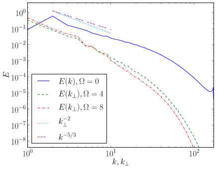
Figure 1: (Color online) Isotropic energy spectrum $E(k)$ in the simulation with $\Omega=0$, and reduced perpendicular energy spectra $E(k_{\perp})$ in the simulations with $\Omega=4$ and $8$. In all three simulations $\textrm{Re}\approx 5000$, while $\textrm{Ro}\approx\infty$, $0.03$, and $0.015$ respectively. Kolmogorov and $\sim k_{\perp}^{-2}$ slopes are shown as a reference. The simulation without rotation has a spectrum with a narrow range of scales arguably compatible with Kolmogorov scaling and followed by a bottleneck and a dissipative range, while the runs with rotation display a steeper spectrum.

In the ideal case and in the absence of forcing, the linearized equations have helical waves ${\bf h}_{s}$ as solutions, with $s=\pm 1$ corresponding to the two possible circular polarizations such that $i{\bf k}\times{\bf h}_{s}=sk{\bf h}_{s}$, and with ${\bf k}$ the wave vector. These waves correspond to inertial waves with dispersion relation $\omega_{\bf k}=s2\Omega k_{z}/k$. The velocity field at wave vector ${\bf k}$ can then be decomposed as Waleffe (1993)

$${\bf u}({\bf k},t)=a_{+}({\bf k},t){\bf h}_{+}+a_{-}({\bf k},t){\bf h}_{-}.$$ (5)

In the nonlinear case, a large number of modes are excited (and nonlinearly coupled) in the velocity field. As a rotating flow can sustain both waves and eddies, for sufficiently strong rotation it is safe to assume that for a large number of wave vectors ${\bf k}$ the waves will be faster than the eddies. Then, in wave turbulence theories the amplitudes $a_{s}({\bf k},t)$ are further decomposed into

$$a_{s}({\bf k},t)=A_{s}(T)e^{i\omega_{\bf k}t},$$ (6)

where $e^{i\omega_{\bf k}t}$ is the fast variation at timescale $\tau_{\omega}=2\pi/\omega_{\bf k}$ associated with the waves, and $A_{s}(T)$ is a slowly varying modulation on a timescale $T\sim\textrm{Ro}\,t$ associated with the eddies.

Replacing this decomposition in Eq. (1), it is obtained that energy is only transferred between modes with wave vectors ${\bf k}$, ${\bf p}$, and ${\bf q}$ such that Cambon and Jacquin (1989); Waleffe (1993); Cambon et al. (1997)

$${\bf k}+{\bf p}+{\bf q}=0,$$ (7)

and

$$\omega_{\bf k}+\omega_{\bf p}+\omega_{\bf q}=0.$$ (8)

The last relation, corresponding to the resonant condition of the waves to have net transfer of energy when integrated over times longer than the wave period, is also associated with the development of anisotropies in the flow. Equation (8) is trivially satisfied for modes with $k_{z}=0$ (the so-called 2D or “slow” modes, as those modes have wave frequency $\omega_{\bf k}=0$), and Eqs. (7) and (8) drive the nonlinear coupling to transfer energy preferentially towards modes with small $k_{z}$ Waleffe (1993). However, the problem with wave turbulence theories is that they are not valid for small values of $k_{z}$, as those modes have eddy turnover times of the order (or faster) than the wave periods. In fact, in many theories the predicted energy transfer towards modes with $k_{z}=0$ vanishes, and 2D modes are then completely decoupled from wave modes Galtier (2003).

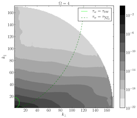
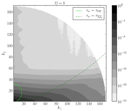
Figure 2: (Color online) Isocontours of the axisymmetric energy spectrum $e(k_{\perp},k_{\parallel})$ in the runs with $\Omega=4$ (above) and $8$ (below); dark means larger energy density (in logarithmic scale). Lines indicating the modes for which the wave time becomes equal to the sweeping time, and to the turnover time, are given as references. It should be noted that the energy does not accumulate near the modes with $\tau_{\omega}=\tau_{\textrm{NL}}$, unlike what is expected in theories dealing with the concept of critical balance Nazarenko and Schekochihin (2011).

At this point, it is important to distinguish more precisely between theories of weak and of strong turbulence. In weak turbulence theory it is assumed that rotation is so strong that nonlinear interactions are weak, such that the linear decorrelation of the waves dominates over any nonlinear decorrelation time. Such theories predict the development of anisotropy and the transfer towards modes with smaller $k_{z}$, but the transfer is arrested as the energy reaches modes with turnover time of the order of the wave period (see, e.g., Galtier (2003)). In theories of strong turbulence (as, e.g., Eddy-Damped Quasi-Normal Markovian, or EDQNM, closures) strong nonlinear coupling can be modeled (although the modes with $k_{z}=0$ still remain decoupled from the other modes), and nonlinear decorrelation times can be dominant Cambon and Jacquin (1989); Cambon et al. (1997); Bellet et al. (2006). However, for the energy to remain positive in such closures a damping time must be externally imposed (see Cambon et al. (2004)). This damping time is often chosen as

$$\frac{1}{\tau_{D}}=\sqrt{\sum_{i}\left(\frac{1}{\tau_{i}}\right)^{2}},$$ (9)

where $\tau_{i}$ are the different times in the system (e.g., viscous, wave, and eddy turnover times), although other empirical combinations can be used Cambon and Jacquin (1989); Cambon et al. (1997); Bellet et al. (2006) to improve the modeling of spectral anisotropy.

Table 1: Fraction of the energy contained in the different regions of ${\bf k}$-space defined in Fig. 2, for the two runs with $\Omega\neq 0$. $\Omega$ is the rotation frequency, $E(\textrm{2D})/E$ is the ratio of energy in the 2D modes to the total energy, $E(\tau_{\omega}<\tau_{\textrm{sw}})/E$ is the fraction of energy in the modes with the wave period faster than the sweeping time, and $E(\tau_{\omega}<\tau_{\textrm{NL}})/E$ is the fraction of the energy in the modes with the wave period faster than the turnover time.

$\Omega$	$E(\textrm{2D})/E$	$E(\tau_{\omega}<\tau_{\textrm{sw}})/E$	$E(\tau_{\omega}<\tau_{\textrm{NL}})/E$
4	0.37	0.59	0.60
8	0.31	0.67	0.68

II.2 Wavenumber-frequency spectrum and correlation functions

Rotating turbulence is often studied using spectra of spatial fluctuations, either isotropic or anisotropic. However, distinction between eddies and waves requires spectra also resolved in frequencies, to distinguish the modes that satisfy the dispersion relation from the rest. There are studies in which the presence of inertial waves was explicitly verified in simulations and experiments Hopfinger et al. (1982); Godeferd and Lollini (1999); Manders and Maas (2003) (including observations of inertial waves in the Earth core Aldridge and Lumb (1987)), although studying their coexistence with turbulent eddies is only possible with large amounts of data. This can be understood as computation of spectra resolved in time and in space require storing data of high resolution simulations (or experiments) with a very short cadence in time (at least twice faster than the fastest waves in the system), and for very long times (at least twice the slowest timescale in the flow).

In the following we present spectra $E_{ij}({\bf k},\omega)$ for several numerical simulations, defined as

$$E_{ij}({\bf k},\omega)=\frac{1}{2}\hat{u}_{i}^{*}({\bf k},\omega)\hat{u}_{j}({\bf k},\omega),$$ (10)

where $\hat{u}_{i}({\bf k},\omega)$ is the Fourier transform in time and in space of the $i$-component of the velocity field ${\bf u}({\bf x},t)$, and where the asterisk denotes complex conjugate.

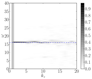
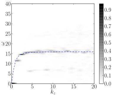
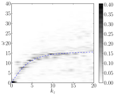
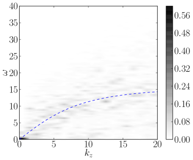
Figure 3: (Color online) Normalized wave vector and frequency spectrum $E_{11}({\bf k},\omega)/E_{11}({\bf k})$ for the run with $\Omega=8$. Darker regions indicate larger energy density. The dashed curve indicates the dispersion relation for inertial waves. Top left: Normalized $E_{11}(k_{x}=0,k_{y}=0,k_{z},\omega)$. Top right: Normalized $E_{11}(k_{x}=0,k_{y}=1,k_{z},\omega)$. Bottom left: Normalized $E_{11}(k_{x}=0,k_{y}=5,k_{z},\omega)$. Bottom right: Normalized $E_{11}(k_{x}=0,k_{y}=10,k_{z},\omega)$. Note from the maximum values in the color bars how the modes close to the dispersion relation concentrate most of the energy in the first two cases ($k_{y}=0$ and $k_{y}=1$), while as $k_{y}$ is increased energy becomes more spread.

Information on the relevant timescales for each spatial mode, and on their decorrelation time, can be obtained also from the time correlation function

$$\Gamma_{ij}({\bf k},\tau)=\frac{\left<\hat{u}_{i}^{*}({\bf k},t)\hat{u}_{j}({\bf k},t+\tau)\right>_{t}}{\left<|\hat{u}_{i}^{*}({\bf k},t)\hat{u}_{j}({\bf k},t)|\right>_{t}},$$ (11)

where $\hat{u}_{i}({\bf k},t)$ is the Fourier transform in space of the $i$-component of the velocity field, the brackets denote time average, and only the real part is used. If the mode $\hat{u}_{i}({\bf k},t)$ is dominated by waves in a regime that satisfies the hypothesis of weak turbulence theory, then $\Gamma_{ii}({\bf k},\tau)\sim\cos(\omega_{\bf k}\tau)$. If nonlinear effects are important, then the mode with wave vector ${\bf k}$ should be decorrelated after a time $\tau_{D}({\bf k})$ following an approximate exponential decay

$$\Gamma_{ii}({\bf k},\tau)\sim e^{-\tau/\tau_{D}({\bf k})}.$$ (12)

In the following we will define $\tau_{D}$ as the time at which the function $\Gamma$ decays to $1/e$ of its initial value. Note this definition is arbitrary, and some authors use the half-width of the correlation function, or a value based on an integral timescale (see, e.g., Favier et al. (2010); Servidio et al. (2011))

$$\tau_{D}({\bf k})=\int_{0}^{\infty}\Gamma_{ii}({\bf k},\tau)\,\text{d}\tau.$$ (13)

We verified that no quantitative differences are obtained by using these other definitions, except for a multiplicative factor of order one in the values of all decorrelation times.

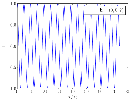
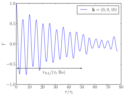
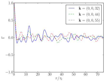
Figure 4: (Color online) Correlation function $\Gamma_{11}(\tau)$ for different modes, the wave-like behavior is quite evident in the first two panels. Time is normalized such that $\Gamma_{11}(\tau)=1/e$ at a time of order unity. See text for the definition of $\tau_{\textrm{t}}$. Top: A mode with $\tau_{\omega}\ll\tau_{\textrm{sw}}$. Middle: A mode with $\tau_{\omega}<\tau_{\textrm{sw}}$. Here $\tau_{\omega}$ still dominates, and the correlation function shows the oscillating behavior expected for a wave-like mode, but with a slow decay in its modulation proportional to the nonlinear time (indicated by the arrow). Bottom: A mode with $\tau_{\omega}>\tau_{\textrm{sw}}$, here all wave-like behavior is lost.

II.3 Numerical simulations

Computation of the functions described above require a significant amount of storage. As a result, only moderate resolution simulations can be performed. We performed three simulations using grids of $N^{3}=512^{3}$ points, in a three-dimensional periodic box.

Equations (1) and (2) were solved using a parallel pseudospectral method, and evolved in time with a second order Runge-Kutta scheme (for more details of the code, see Gómez et al. (2005); Mininni et al. (2011)). The simulations were dealiased with the $2/3$-rule (see, e.g., Gómez et al. (2005)).

The equations are written in dimensionless units. The periodic domain has length $\lambda_{0}=2\pi$, resulting in integer wavenumbers and in a minimum wave number $k_{\textrm{min}}=2\pi/\lambda_{0}=1$. Per virtue of the $2/3$-rule, the largest resolved wave number is $k_{\textrm{max}}=N/3$, associated with the smallest resolved wavelength $\lambda_{\textrm{min}}=2\pi/k_{\textrm{max}}=6\pi/N$. With this choice, for a characteristic velocity $U_{0}=1$ and a characteristic length $L_{0}=1$, the turnover time is $T_{0}=L_{0}/U_{0}=1$, which we use as unit of time. $\Omega$ is then measured in units of the inverse of time $T_{0}$.

In previous studies of rotating turbulence in periodic domains, it was found that if the forcing is applied at intermediate scales (i.e., scales smaller than the size of the domain), an inverse cascade develops and most of the energy ends up in the 2D modes Sen et al. (2012). Evidence of this inverse cascade has been also observed in experiments Yarom et al. (2013). It is unclear for the moment whether this effect also takes place in homogeneous, unbounded flows, such as those considered by wave turbulence theories Cambon et al. (2004). As a result, we forced the system at the largest scales available, to prevent the inverse cascade from developing. However, this has a caveat: the finite domain selects a discrete set of inertial waves which are normal modes of the domain (see, e.g., Smith and Lee (2005); Bellet et al. (2006)). As a result of the discretized wavenumbers, the number of modes that satisfy the resonance condition (8) depends on the wavenumber, and is smaller (or zero) for smaller wavenumbers, resulting in only near-resonances being available Smith and Lee (2005). As this effect is aggravated when domains with non-unity aspect ratio are used, we restricted our study to boxes with aspect ratio of unity.

As we are also interested in correlation times, to prevent imposing external correlation times with the forcing we used a coherent forcing (in opposition to a time-correlated, or delta-correlated in time forcing function). We therefore used Taylor-Green forcing

$${\bf F} = F_{0}\left[\sin(k_{\textrm{TG}}x)\cos(k_{\textrm{TG}}y)\cos(k_{\textrm{TG}}z)\hat{x}\right.$$ (14)

$$\left.-\cos(k_{\textrm{TG}}x)\sin(k_{\textrm{TG}}y)\cos(k_{\textrm{TG}}z)\hat{y}\right],$$

where $F_{0}$ is the amplitude of the force, which was kept constant in time. Although the forcing injects energy directly only into the $x$- and $y$-components of the velocity, the resulting flow is three-dimensional because of pressure gradients that excite the remaining component of the velocity field. This forcing injects no energy in the 2D modes, and only affects directly a few modes in Fourier space corresponding (for the choice $k_{\textrm{TG}}=1$) to the mode ${\bf k}=(1,1,1)$ in the first quadrant, and the modes obtained after reflections across the axes in Fourier space. As will become evident later, forcing only these modes is better for the excitation of waves than forcing, e.g., all modes in a spherical shell in Fourier space. Finally, Taylor-Green forcing is of interest as it mimics the flow generated in some experiments using two counter-rotating disks Bourgoin et al. (2002); Ponty et al. (2005).

As explained above, the forcing was applied at modes such as ${\bf k}=(1,1,1)$, which results in a forced wave number $k_{\textrm{F}}=|{\bf k}|=\sqrt{3}$, and in a forced length scale $L=2\pi/k_{\textrm{F}}=2\pi/\sqrt{3}$. The amplitude of the force was $F_{0}=0.277$ in all the runs, and this value was chosen to have an r.m.s. velocity close to 1 in the turbulent steady state in the absence of rotation (in practice, $U\approx 0.9$ and fluctuates around this value in time). The kinematic viscosity was $\nu=6.5\times 10^{-4}$, resulting in a Reynolds number in the turbulent steady state $\textrm{Re}\approx 5000$.

Three runs were done using the following procedure. First, a simulation with no rotation ($\Omega=0$) was done starting from the fluid at rest (${\bf u}=0$), and applying the Taylor-Green forcing until the system reached a turbulent steady state. This run was continued for $12$ large scale turnover times. Using the final state of this run as an initial condition, two other runs were done, respectively with $\Omega=4$ and $8$, and keeping the external force and all other parameters the same. Both runs were also evolved for $12$ large scale turnover times. This results in three runs with Rossby numbers respectively of $\textrm{Ro}\approx\infty$, $0.03$, and $0.015$. The last $6$ turnover times of each run (in all cases, after the system reached the turbulent steady state) were used to compute the spectra and correlation functions presented below. For the analysis, data was saved with a time cadence $\Delta t=0.01$.

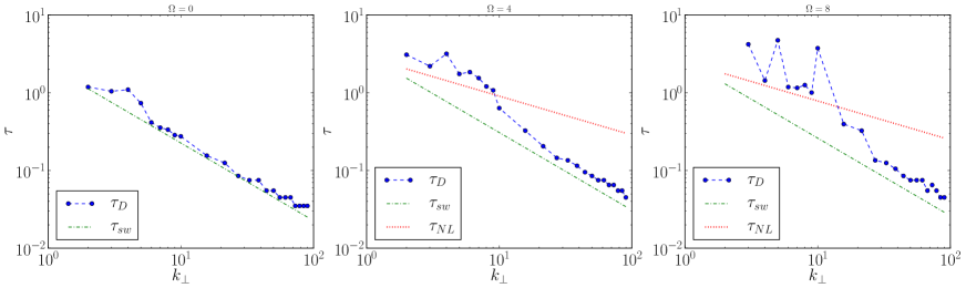
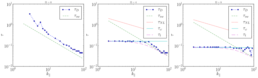
Figure 5: (Color online) Top: Decorrelation time $\tau_{D}$ for the modes with $k_{\parallel}=0$, as a function of $k_{\perp}$, and for the three different values of $\Omega$. Bottom: Same for the modes with $k_{\perp}=0$, as a function of $k_{\parallel}$. In all figures, the data corresponds to the dots connected by dashed lines; the wave period $\tau_{\omega}$, the sweeping time $\tau_{\textrm{sw}}$, the nonlinear time $\tau_{\textrm{NL}}$, and the total effective time $\tau_{\textrm{t}}$ are given as references.

III Analysis

III.1 Behavior of the runs in wavenumber space

Before proceeding to the analysis of the wavenumber and frequency spectrum, and to the study of the decorrelation time for each mode, we present some spectra in wavenumber space, as is often done to characterize turbulent flows. Besides being useful to characterize the runs, these spectra will be also important to identify the behavior of the different modes depending on what dynamical times are expected to be dominant.

Figure 1 shows the isotropic energy spectrum $E(k)$ for the run with $\Omega=0$, and the reduced perpendicular energy spectrum $E(k_{\perp})$ for the two runs with rotation. The reduced perpendicular spectrum is obtained by integrating the power spectrum of $\hat{\bf u}({\bf k},t)$ over cylindrical shells around the axis of rotation, and averaging in time to obtain a spectrum that depends only on $k_{\perp}=\sqrt{k_{x}^{2}+k_{y}^{2}}$. In the absence of rotation, the isotropic spectrum has a narrow range of wave numbers compatible with Kolmogorov scaling, followed by a bottleneck and a dissipative range. In the rotating case the spectrum becomes steeper, as expected.

The axisymmetric energy spectrum $e(k_{\perp},k_{\parallel})$, obtained after integrating the power of $\hat{\bf u}({\bf k},t)$ only over the azimuthal angle in Fourier space, provides more information on the anisotropy of the flow. As rotation is along the $z$ axis, $k_{\parallel}=k_{z}$. Figure 2 shows contour plots of $e(k_{\perp},k_{\parallel})/\sin(\theta_{k})$ for the runs with $\Omega=4$ and with $\Omega=8$, and where $\theta_{k}=\arctan(k_{\perp}/k_{\parallel})$ is the colatitude in Fourier space. For an isotropic flow ($\Omega=0$), contours of $e(k_{\perp},k_{\parallel})/\sin(\theta_{k})$ are circles. As rotation is increased, energy becomes more concentrated near the axis with $k_{\parallel}=0$.

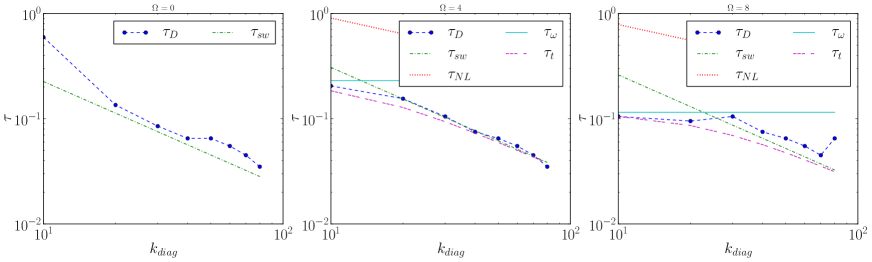
Figure 6: (Color online) Top: Decorrelation time $\tau_{D}$ for the modes with $k_{\perp}=k_{\parallel}$, as a function of $k=\sqrt{k_{\perp}^{2}+k_{\parallel}^{2}}$. Labels for the curves are as in Fig. 5.

Based on the previous discussion on wave turbulence theory, and on previous studies of decorrelation times in isotropic turbulence Chen and Kraichnan (1989); Nelkin and Tabor (1990); Sanada and Shanmugasundaram (1992) and in rotating flows Favier et al. (2010), we can expect several timescales to be relevant for our studies. These timescales depend on the wave vector, and assuming the shorter one dominates the dynamics, different regions in the axisymmetric energy spectrum $e(k_{\perp},k_{\parallel})$ can be defined. The first timescale is the period of the waves

$$\tau_{\omega}({\bf k})=C_{\omega}\frac{k}{2\Omega k_{\parallel}},$$ (15)

where $C_{\omega}$ is a dimensionless constant of order unity.

This time should be compared with the eddy turnover time $\tau_{\textrm{NL}}\sim 1/[k\sqrt{kE(k)}]$. Simple phenomenological arguments suggest the isotropic energy spectrum in the inertial range of rotating turbulence follows $E(k)\sim\epsilon^{1/2}\Omega^{1/2}k^{-2}$ Zhou (1995); Müller and Thiele (2007); Mininni et al. (2012). Then, a possible estimation of the eddy turnover time is

$$\tau_{\textrm{NL}}({\bf k})=C_{\textrm{NL}}\frac{1}{\epsilon^{1/4}\Omega^{1/4}k^{1/2}},$$ (16)

where $C_{\textrm{NL}}$ is another dimensionless constant of order unity, and where $\epsilon$ is the energy injection rate. It is worth noticing that the spectrum of rotating turbulence is actually anisotropic and dependent on $k_{\parallel}$ and $k_{\perp}$ instead of simply on $k$. However, for the purpose of the discussion here, and as we are only concerned with order of magnitude estimation of the timescales, we will use the simplest isotropic expression of $E(k)$.

Sweeping may be the dominant process in the decorrelation of Fourier modes when the sweeping time becomes shorter than the wave period, as is the case in isotropic turbulence Tennekes (1975); Chen and Kraichnan (1989); Nelkin and Tabor (1990); Sanada and Shanmugasundaram (1992), and as also found in simulations of rotating turbulence at lower resolution Favier et al. (2010). The sweeping time is

$$\tau_{\textrm{sw}}({\bf k})=C_{\textrm{sw}}\frac{1}{Uk},$$ (17)

where $C_{\textrm{sw}}$ is a dimensionless constant of order unity. Finally, phenomenological theories of rotating turbulence (see, e.g., Zhou (1995); Müller and Thiele (2007); Mininni et al. (2012)) often also consider an energy cascade transfer time $\tau_{\textrm{tr}}\sim\tau_{\textrm{NL}}(\tau_{\textrm{NL}}/\tau_{\omega})$, where the ratio of timescales between parenthesis expresses the fact that waves slow down the energy cascade.

In Fig. 2 we indicate two curves, corresponding to the modes that satisfy the relations $\tau_{\omega}({\bf k})=\tau_{\textrm{sw}}({\bf k})$, and $\tau_{\omega}({\bf k})=\tau_{\textrm{NL}}({\bf k})$. Modes inside the region enclosed by the former curve have the wave period faster than any other time, and we should expect correlation functions $\Gamma_{ii}({\bf k},\tau)$ for these modes to be harmonic. Modes outside that region should decorrelate with the fastest time, which is the sweeping time. Finally, modes outside the region enclosed by the latter curve have the eddy turnover time shorter than the wave period, and as a result those modes cannot be considered as waves slowly modulated by eddies. In fact, for those modes the effect of rotation should be negligible. These considerations will be important in the next subsection. To plot the curves $\tau_{\omega}({\bf k})=\tau_{\textrm{sw}}({\bf k})$ and $\tau_{\omega}({\bf k})=\tau_{\textrm{NL}}({\bf k})$, we used $C_{\omega}=1.3$, $C_{\textrm{NL}}=1$, $C_{\textrm{sw}}=2.3$; these values were obtained from the analysis of the data in Sec. III.3.

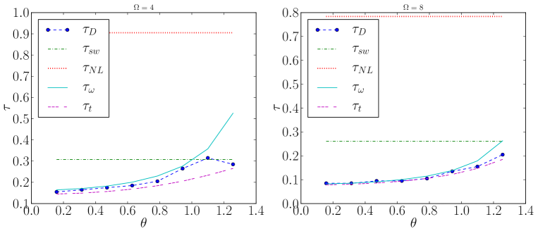
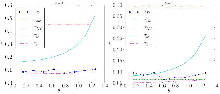
Figure 7: (Color online) Decorrelation time $\tau_{D}$ for modes with $k=$constant, as a function of $\theta_{k}$ (the colatitude in Fourier space). Top: $\tau_{D}(\theta_{k})$ for $k=10$. Bottom: Same for $k=40$. Labels for the curves are as in Fig. 5.

In table 1 the fraction of the energy that is contained in 2D modes, in modes with $\tau_{\omega}<\tau_{\textrm{sw}}$, and in modes with $\tau_{\omega}<\tau_{\textrm{NL}}$ is shown for the simulations with $\Omega=4$ and 8. As mentioned previously, energy becomes more concentrated near the axis with $k_{\parallel}=0$ in the presence of rotation. However, the fraction of the energy in 2D modes actually decreases as $\Omega$ is increased from 4 to 8, and more of the injected energy remains in the modes with $\tau_{\omega}<\tau_{\textrm{sw}}$ (although a significant portion of the energy, $\approx 30\%$, still escapes outside this region and concentrates in the 2D modes). The energy that is concentrated in these modes comes solely from the leakage from the 3D modes, as no energy is injected directly into the 2D modes by the forcing we are using.

The final motivation to use Taylor-Green forcing now becomes apparent. The modes excited by the forcing are in the region $\tau_{\omega}<\tau_{\textrm{sw}}$, and favors modes dominated by the waves. As a result, all energy in the region with $\tau_{\omega}>\tau_{\textrm{sw}}$, and in the region with $\tau_{\omega}>\tau_{\textrm{NL}}$, can only be accounted for by the nonlinear transfer of energy from the modes dominated by the wave time. Weak turbulence theories Galtier (2003) cannot account for this transfer.

It should also be noted that in Fig. 2 the energy does not accumulate near the modes with $\tau_{\omega}=\tau_{\textrm{NL}}$, as it is expected in theories dealing with the concept of critical balance Nazarenko and Schekochihin (2011). In critical balance, it is argued that in the case of strong turbulence, energy in the weak turbulence modes cascades towards larger values of $k_{\perp}$, while energy in modes with $\tau_{\omega}<\tau_{\textrm{NL}}$ (which are outside the domain of weak turbulence, and are, therefore, strong) cascade inversely towards smaller values of $k_{\perp}$ Nazarenko and Schekochihin (2011); Nazarenko (2011). This establishes a balance with $\tau_{\omega}=\tau_{\textrm{NL}}$; energy accumulates in the modes that satisfy this balance and then cascades towards larger values of $k$ along this curve. No such accumulation is visible in Fig. 2, and as only modes with $\tau_{\omega}<\tau_{\textrm{sw}}$ are forced, the energy in the domain $\tau_{\omega}>\tau_{\textrm{NL}}$ can only come from a transfer from the wave modes to the vortical modes in the direction opposite to that needed to establish the balance.

III.2 Wave vector and frequency spectrum

Figure 3 shows the wave vector and frequency spectrum $E_{11}({\bf k},\omega)/E_{11}({\bf k})$ for different values of ${\bf k}$, where

$$E_{11}(\mathbf{k})=\int E_{11}({\bf k},\omega)\,\text{d}\omega.$$ (18)

With this choice for the normalization, the frequencies that concentrate most of the energy for each ${\bf k}$ are more clearly visible.

When $k_{x}=0$, $k_{y}=0$, and $k_{z}$ is varied, most of the energy is concentrated near $\omega=2\Omega$, especially for $k_{z}<10$. For larger values of $k_{z}$ the width of the band that concentrates most of the energy increases (compare this with the regions in Fig. 2 corresponding to modes with $\tau_{\omega}({\bf k})<\tau_{\textrm{sw}}({\bf k})$, and to modes with $\tau_{\omega}({\bf k})<\tau_{\textrm{NL}}$). The wave vector and frequency spectrum for the other components of the velocity were also calculated, showing similar behavior.

When $k_{x}=0$, $k_{y}$ is kept fixed, and $k_{z}$ is varied, most of the energy is still concentrated near the linear dispersion relation $\omega=2\Omega k_{z}/\sqrt{k_{y}^{2}+k_{z}^{2}}$ in the cases with $k_{y}=1$ and $k_{y}=5$. However, for $k_{y}=10$ and larger, energy is more evenly distributed among all values of $\omega$, and most of the energy is in the modes with $\omega\approx 0$.

Leaving aside the energy in the modes with $\omega\approx 0$, the modes that concentrate energy near the linear dispersion relation could in principle be treated by weak turbulence theories, where energy is transferred through wave interactions. But it is worth pointing out also that the accumulation of energy in these fast modes makes (at least for a subset of the wave numbers) some magnitudes in the turbulent flow treatable by RDT Cambon and Jacquin (1989); Cambon and Scott (1999). This has been used to study the early time evolution of the system when rotation is turned on in an initially isotropic flow Brethouwer (2005)).

III.3 Correlation functions and decorrelation times

Figure 4 shows the time correlation function $\Gamma_{11}({\bf k},\tau/\tau_{t})$ for the $x$-component of the velocity, with the time being normalized by a total effective time $\tau_{t}$, and for different modes in Fourier space. The total effective time is defined as

$$\left(\frac{1}{\tau_{\textrm{t}}}\right)^{2}=\left(\frac{1}{\tau_{\omega}}\right)^{2}+\left(\frac{1}{\tau_{\textrm{sw}}}\right)^{2},$$ (19)

such that for $\tau_{\omega}\ll\tau_{\textrm{sw}}$, $\tau_{\textrm{t}}\approx\tau_{\omega}$, and for $\tau_{\omega}\gg\tau_{\textrm{sw}}$, $\tau_{\textrm{t}}\approx\tau_{\textrm{sw}}$. With this definition, $\Gamma_{11}(\tau/\tau_{t})=1/e$ at a time $\tau/\tau_{t}$ of order unity for all modes.

By inspection of these functions, we identified three different behaviors that are illustrated by a few modes in the figure. Modes near the $k_{\parallel}$ axis (and for sufficiently small $k_{\parallel}$) have $\Gamma\sim\cos(\omega_{\bf k}\tau)$, the behavior expected for waves ($\tau_{t}\approx\tau_{\omega}$ for these wavenumbers). As $k_{\parallel}$ is increased (and as $k_{\perp}$ is increased as well), the correlation functions still show a wave-like behavior, but also display a slower decay in their modulation in a time that can be associated with the eddy timescale $\tau_{\textrm{NL}}$ (following Eq. 6, the eddy or “slow” timescale $T$ is of order one when $t\sim{Ro}^{-1}$; in that timescale the decay time of the correlation functions is given by $\tau_{\textrm{NL}}$). It is interesting that the slow modulation takes place on a timescale of the order of ${Ro}^{-1}$, as some studies suggest that this is the time in which energy is transfered outside the region of weak turbulence in Fourier space, and for which rotating turbulence becomes strong Chen et al. (2005). Finally, for even larger values of the wavenumber, the correlation functions decay exponentially and resemble those obtained in the absence of rotation. Correlation functions for the other components of the velocity were also calculated, showing similar behavior.

From the correlation functions the decorrelation time $\tau_{D}$ can be measured directly. Figure 5 shows $\tau_{D}$ for the $x$-component of the velocity for modes along the $k_{y}$ axis (i.e., for $k_{x}=k_{z}=0$), and along the $k_{z}$ axis (i.e., for $k_{x}=k_{y}=0$). In the case with $k_{\parallel}=0$, the modes seem to decorrelate with the sweeping time independently of the value of $\Omega$, as also found in Favier et al. (2010), although in the rotating case and for small $k_{\perp}$ ($k_{\perp}\lesssim 10$) the behavior seems to be compatible with $\tau_{D}\sim\tau_{\textrm{NL}}$. Note that in the runs with rotation, these modes correspond to the 2D or “slow” modes, with zero wave frequency. As a result, these modes can only be vortical.

The modes with $k_{\perp}=0$ decorrelate with the sweeping time in the run without rotation, but in the runs with rotation $\tau_{D}$ has a transition at $\tau_{\omega}({\bf k})=\tau_{\textrm{sw}}({\bf k})$. For $k_{\parallel}$ such that $\tau_{\omega}({\bf k})<\tau_{\textrm{sw}}({\bf k})$, $\tau_{D}\approx\tau_{\omega}$. For $k_{\parallel}$ such that $\tau_{\omega}({\bf k})>\tau_{\textrm{sw}}({\bf k})$, $\tau_{D}\approx\tau_{\textrm{sw}}$. This transition was also found in the simulations in Favier et al. (2010). The nonlinear time plays no clear role in the decorrelation. A similar behavior is obtained if ${\bf k}$ is varied along the diagonal with $k_{y}=k_{z}$ and $k_{x}=0$ (see Fig. 6), or if $k$ is kept fixed and the colatitude $\theta_{k}$ in Fourier space is varied (see Fig. 7). This former case is interesting as for small values of $k$ the decorrelation time $\tau_{D}$ is closer to the wave period, while for larger values of $k$ the decorrelation is closer to the sweeping time (i.e., approximately constant with $\theta_{k}$). As explained above, the modes dominated by the faster timescale $\tau_{\omega}$ satisfy conditions akin to the hypothesis made in RDT Cambon and Jacquin (1989); Cambon and Scott (1999).

The dimensionless constants $C_{\omega}$, $C_{\textrm{NL}}$, and $C_{\textrm{sw}}$ in Eqs. (15), (16), and (17) were chosen from the data in Figs. 5, 6, and 7, and are the same for all runs (independently of the mode ${\bf k}$ studied, and of the value of $\Omega$). Note these amplitudes only account for an arbitrariness in the definition of the decorrelation time, which from the time correlation function and as explained above can be defined based on the time to decay to $1/e$ of its value, based on its half-width, or on an integral timescale.

From these observations, it becomes apparent that the effective time $\tau_{t}$ gives a good approximation to the actual decorrelation time $\tau_{D}$ in all figures. It is interesting that the choice to average the relevant times in Eq. (19) is similar to the choice used in the simplest EDQNM models of rotating turbulence to estimate the eddy damping Cambon and Jacquin (1989); Cambon et al. (1997).

From these figures, we can also conclude that the modes in the region enclosed by the curve $\tau_{\omega}=\tau_{\textrm{sw}}$ in Fig. 2 have wave-like behavior with decorrelation dominated by the waves, while the rest of the modes are dominated by sweeping effects (similar to what happens in isotropic and homogeneous turbulence Chen and Kraichnan (1989)).

III.4 Decorrelation times and anisotropy

The fact that modes with $\tau_{\omega}>\tau_{\textrm{sw}}$ have decorrelation dominated by the sweeping time should not be interpreted as that the effects of waves and of rotation are negligible for these modes. This is evidenced quite clearly in Fig. 2, where anisotropic spectral distribution of energy can be observed even for modes with $\tau_{\omega}>\tau_{\textrm{sw}}$. Isotropy is expected to be recovered at the Zeman wavenumber $k_{\Omega}$ for which $\tau_{\omega}(k_{\Omega})=\tau_{\textrm{NL}}(k_{\Omega})$ Zeman (1994). This wavenumber is equivalent to the Ozmidov wavenumber in a stratified flow, and that isotropy is recovered in rotating turbulence at that wave number has been recently confirmed in high resolution numerical simulations Mininni et al. (2012).

From the expressions in Sec. III.1, assuming that when isotropy is recovered $k_{\perp}\approx k_{\parallel}$ and therefore $k\approx\sqrt{2}k_{\parallel}$, we can write the condition $\tau_{\omega}=\tau_{\textrm{NL}}$ at $k=k_{\Omega}$ as

$$\frac{C_{\textrm{NL}}}{\epsilon^{1/4}\Omega^{1/4}k^{1/2}_{\Omega}} =\frac{C_{\omega}}{\sqrt{2}\Omega}$$

$$\Rightarrow k_{\Omega} =C_{\Omega}\left(\frac{\Omega^{3}}{\epsilon}\right)^{1/2},$$

where $C_{\Omega}=2(C_{\textrm{NL}}/C_{\omega})^{2}\approx 1.18$.

This expression is compatible with the one found in Mininni et al. (2012), where $C_{\Omega}=1$ was found from direct observation of the scale at which isotropy was recovered. For the simulation with $\Omega=4$, $k_{\Omega}\approx 150$ (which lies in the dissipative range of the simulation), and for the simulation with $\Omega=8$, $k_{\Omega}\approx 460$ (which lies outside the domain of resolved scales).

It is interesting that the characteristic timescales discussed here present another interpretation of the Zeman scale: isotropy is recovered not when all modes satisfy the condition $\tau_{\textrm{NL}}\leq\tau_{\omega}$ (which happens in the runs with $\Omega=4$ and $8$ at much larger wave numbers, see Fig. 2), but when a significant fraction of the modes satisfy this condition (i.e., when the modes in the diagonal with $k_{\perp}\approx k_{\parallel}$ satisfy the equality of timescales).

IV Conclusions

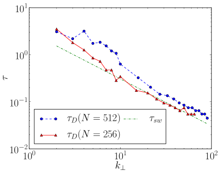
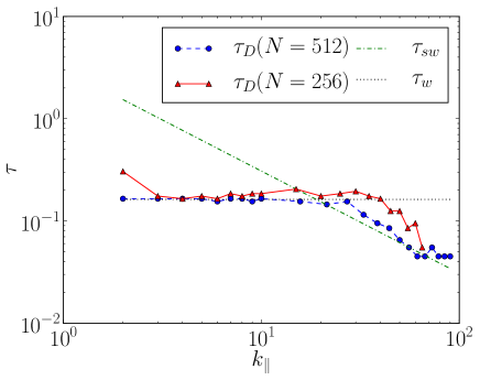
Figure 8: (Color online) Top: Decorrelation time $\tau_{D}$ for the modes with $k_{\parallel}=0$ as a function of $k_{\perp}$, for runs with same value of $\Omega$ but different spatial resolution $N$ and Reynolds number. The time $\tau_{D}(N=512)$ is for the run with $N=512$ linear resolution, while $\tau_{D}(N=256)$ is for the run with $N=256$. Bottom: Same for the modes with $k_{\perp}=0$, as a function of $k_{\parallel}$. In all figures, the data corresponds to the symbols connected by dashed lines. The curves scaling with wavenumber as the wave period $\tau_{\omega}$, the sweeping time $\tau_{\textrm{sw}}$, and the total effective time $\tau_{\textrm{t}}$ are shown as references.

The results presented here indicate that: (1) A significant fraction of the energy is concentrated in modes with $\omega\approx 0$, which have correlation functions corresponding to that of strong turbulence (i.e., vortical modes). In this respect, the simulations are limited to finite domains and we cannot conclude from this what the behavior is for a homogeneous (infinite) flow as is often considered in wave turbulence theories. (2) For modes with $\tau_{\omega}\ll\tau_{\textrm{sw}}$, a significant fraction of the remaining energy is concentrated near the dispersion relation $\omega({\bf k})$ of inertial waves. However, the dispersion relation is not visible anymore in $E({\bf k},\omega)$ as the wave number is increased. (3) For $\tau_{\omega}<\tau_{\textrm{sw}}$, the correlation functions behave as expected for modes in weak turbulence theories: waves slowly modulated by eddies. For $\tau_{\omega}\ll\tau_{\textrm{sw}}$, waves dominate and the correlation functions are harmonic in $\tau$. The rest of the modes decorrelate with the sweeping time. However, the effects of rotation only become negligible (e.g., to reobtain isotropy) for modes with $\tau_{\textrm{NL}}\leq\tau_{\omega}$.

Previous studies of the time correlation function at lower Reynolds number and at lower spatial resolution, using $256^{3}$ grid points, obtanied similar results Favier et al. (2010). This indicates that the results are not very sensitive to the value of the Reynolds number, at least in the range of parameters considered in the present study. To further confirm this, in the Appendix we present a comparison of our results with simulations with $256^{3}$ grid points and with $\textrm{Re}\approx 3100$. Studying flows with higher Reynolds numbers is currently out of our reach, as computation of time correlation functions and of the wave number and frequency spectrum require storage of vast amounts of data which increase rapidly as spatial resolution is increased. Such higher Reynolds numbers studies would determine the degree of applicability of the current results to the fully developed turbulence regime.

Finally, the results presented here were obtained for a forcing function that only excites a few modes in the region of Fourier space dominated by the wave timescale. For isotropic, random, delta-correlated in time forcing, preliminary studies indicate that at the same Rossby number the effect of the waves is weaker.

*

Appendix A Simulations with lower Reynolds number

We briefly compare here the results obtained from the simulations with $512^{3}$ grid points and $\textrm{Re}\approx 5000$, with simulations at lower resolution and lower Reynolds number. We performed a set of simulations with the same Rossby numbers as the $512^{3}$ simulations, but with larger viscosity and using $N^{3}=256^{3}$ grid points, resulting in a Reynolds number $\textrm{Re}\approx 3100$.

Figure 8 presents a comparison of the decorrelation times in the simulations with $256^{3}$ and $512^{3}$ grid points, both with $\Omega=4$. This figure is equivalent to Fig. 5, in which only the results for the $512^{3}$ simulation were shown. The sweeping time and the wave period are the same for both simulations, as the forcing amplitude and the value of $\Omega$ were kept the same. No significative differences are observed between both simulations, and the decorrelation time presents the same behavior with $k_{\parallel}$ and $k_{\perp}$ in both cases. Small differences observed are due to the fact that the r.m.s. velocity is not exactly the same in both runs.

We also verified that other quantities (such as $\Gamma_{11}$, the correlation functions) also act similarly in the $\textrm{Re}=3100$ and $\textrm{Re}=5000$ cases, lending some confidence that the results described above are not very sensitive to the Reynolds number at the modest values considered here.

References

- Cambon et al. (2004) C. Cambon, R. Rubinstein, and F. S. Godeferd, New J. Phys. 6, 73 (2004).
- Cambon and Jacquin (1989) C. Cambon and L. Jacquin, J. Fluid Mech. 202, 295 (1989).
- Cambon et al. (1997) C. Cambon, N. N. Mansour, and F. S. Godeferd, J. Fluid Mech. 337, 303 (1997).
- Bellet et al. (2006) F. Bellet, F. S. Godeferd, and F. S. Scott, J. Fluid Mech. 562, 83 (2006).
- Waleffe (1993) F. Waleffe, Phys. Fluids A 5, 677 (1993).
- Galtier (2003) S. Galtier, Phys. Rev. E 68, 015301 (2003).
- Chen et al. (2005) Q. Chen, S. Chen, G. L. Eyink, and D. Holm, J. Fluid Mech. 542, 139 (2005).
- Müller and Thiele (2007) W.-C. Müller and M. Thiele, Europhys. Lett. 77, 34003 (2007).
- Mininni et al. (2009) P. D. Mininni, A. Alexakis, and A. Pouquet, Phys. Fluids 21, 015108 (2009).
- Mininni et al. (2012) P. D. Mininni, D. Rosenberg, and A. Pouquet, J. Fluid Mech. 699, 263 (2012).
- Cobelli et al. (2009) P. Cobelli, P. Petitjeans, A. Maurel, V. Pagneux, and N. Mordant, Phys. Rev. Lett. 103, 204301 (2009).
- Cobelli et al. (2011) P. Cobelli, A. Przadka, P. Petitjeans, G. Lagubeau, V. Pagneux, and A. Maurel, Phys. Rev. Lett. 107, 214503 (2011).
- Dmitruk and Matthaeus (2009) P. Dmitruk and W. H. Matthaeus, Phys. Plasmas 16, 062304 (2009).
- Cambon and Scott (1999) C. Cambon and J. F. Scott, Annual review of fluid mechanics 31, 1–53 (1999).
- Durbin and Reif (2011) P. A. Durbin and B. A. P. Reif, Statistical theory and modeling for turbulent flow (Wiley, Chichester, West Sussex, UK, 2011).
- Favier et al. (2010) B. Favier, F. S. Godeferd, and C. Cambon, Phys. Fluids 22, 015101 (2010).
- Servidio et al. (2011) S. Servidio, V. Carbone, P. Dmitruk, and W. H. Matthaeus, EPL (Europhysics Letters) 96, 55003 (2011).
- Tennekes (1975) H. Tennekes, Journal of Fluid Mechanics 67, 561–567 (1975).
- Chen and Kraichnan (1989) S. Chen and R. H. Kraichnan, Physics of Fluids A: Fluid Dynamics 1, 2019 (1989).
- Nelkin and Tabor (1990) M. Nelkin and M. Tabor, Phys. Fluids A 2, 81 (1990).
- Sanada and Shanmugasundaram (1992) T. Sanada and V. Shanmugasundaram, Phys. Fluids A 4, 1245 (1992).
- Monin and Yaglom (2007) A. S. Monin and A. M. Yaglom, Statistical fluid mechanics mechanics of turbulence. (Dover Publications, New York, 2007).
- Blackman and Field (2003) E. G. Blackman and G. B. Field, Phys. Fluids 15, L73 (2003).
- Nazarenko and Schekochihin (2011) S. V. Nazarenko and A. A. Schekochihin, J. Fluid Mech. 677, 134–153 (2011).
- Hopfinger et al. (1982) E. J. Hopfinger, F. K. Browand, and Y. Gagne, J. Fluid Mech. 125, 505 (1982).
- Godeferd and Lollini (1999) F. S. Godeferd and L. Lollini, J. Fluid Mech. 393, 257 (1999).
- Manders and Maas (2003) A. M. M. Manders and L. R. M. Maas, J. Fluid Mech. 493, 59 (2003).
- Aldridge and Lumb (1987) K. D. Aldridge and I. Lumb, Nature 325, 421 (1987).
- Gómez et al. (2005) D. O. Gómez, P. D. Mininni, and P. Dmitruk, Adv. Sp. Res. 35, 899 (2005).
- Mininni et al. (2011) P. D. Mininni, D. Rosenberg, R. Reddy, and A. Pouquet, Parallel Computing 37, 316 (2011).
- Sen et al. (2012) A. Sen, P. D. Mininni, D. Rosenberg, and A. Pouquet, Phys. Rev. E 86, 036319 (2012).
- Yarom et al. (2013) E. Yarom, Y. Vardi, and E. Sharon, Phys. Fluids 25, 085105 (2013).
- Smith and Lee (2005) L. M. Smith and Y. Lee, J. Fluid Mech. 535, 111 (2005).
- Bourgoin et al. (2002) M. Bourgoin, L. Marié, F. Pétrélis, C. Gasquet, A. Guigon, J.-B. Luciani, M. Moulin, F. Namer, J. Burguete, A. Chiffaudel, F. Daviaud, S. Fauve, P. Odier, and J.-F. Pinton, Phys. Fluids 14, 3046 (2002).
- Ponty et al. (2005) Y. Ponty, P. D. Mininni, D. C. Montgomery, J.-F. Pinton, H. Politano, and A. Pouquet, Phys. Rev. Lett. 94, 164502 (2005).
- Zhou (1995) Y. Zhou, Phys. Fluids 7, 2092 (1995).
- Nazarenko (2011) S. Nazarenko, Wave Turbulence (Springer-Verlag, Berlin, 2011).
- Brethouwer (2005) G. Brethouwer, Journal of Fluid Mechanics 542, 305 (2005).
- Zeman (1994) O. Zeman, Phys. Fluids 6, 3221 (1994).