Chimera: A hybrid approach to numerical loop quantum cosmology

Abstract

The existence of a quantum bounce in isotropic spacetimes is a key result in loop quantum cosmology (LQC), which has been demonstrated to arise in all the models studied so far. In most of the models, the bounce has been studied using numerical simulations involving states which are sharply peaked and which bounce at volumes much larger than the Planck volume. An important issue is to confirm the existence of the bounce for states which have a wide spread, or which bounce closer to the Planck volume. Numerical simulations with such states demand large computational domains, making them very expensive and practically infeasible with the techniques which have been implemented so far. To overcome these difficulties, we present an efficient hybrid numerical scheme using the property that at the small spacetime curvature, the quantum Hamiltonian constraint in LQC, which is a difference equation with uniform discretization in volume, can be approximated by a Wheeler-DeWitt differential equation. By carefully choosing a hybrid spatial grid allowing the use of partial differential equations at large volumes, and with a simple change of geometrical coordinate, we obtain a surprising reduction in the computational cost. This scheme enables us to explore regimes which were so far unachievable for the isotropic model in LQC. Our approach also promises to significantly reduce the computational cost for numerical simulations in anisotropic LQC using high performance computing.

1 Introduction

A key prediction of loop quantum gravity (LQG) is that classical differential geometry of general relativity (GR) is replaced by discrete quantum geometry at the Planck scale. Loop quantum cosmology (LQC) which is a quantization of homogeneous spacetimes based on LQG, manifests this feature in the form of a discrete quantum evolution equation which is non-singular [1]. Due to the quantum geometric effects, the energy density and curvature invariants are bounded and the classical big bang is replaced by a quantum big bounce. At curvature scales far smaller than the Planck scale, the quantum evolution equation, a finite difference equation in volume, can be well approximated by the Wheeler-DeWitt (WDW) differential equation, and GR is recovered in the infra-red regime. The smooth classical differential geometry of classical GR turns out to be a low curvature approximation of the underlying quantum geometry.

The existence of a bounce in LQC was first demonstrated for the case of a spatially flat $(k=0)$, homogeneous and isotropic model sourced with a massless scalar field [3, 4, 5]. In these papers, numerical simulations are performed with an appropriate choice of an initial state peaked on a classical trajectory at late times. Such a state is then evolved backwards in internal time towards the big bang using the loop quantum difference equation. In the numerical evolution, the LQC trajectory agrees with the classical trajectory as long as the spacetime curvature remains much below the Planck curvature. As the backward evolution continues, and the curvature increases, the quantum geometric effects become more prominent. As a result, the LQC trajectory starts to deviate from the classical trajectory, eventually resulting in a bounce which occurs when the energy density of the massless scalar field reaches a maximum value $\rho_{\mathrm{max}}\approx 0.41\rho_{\mathrm{Planck}}$. Further, for states which are semi-classical at late times in a macroscopic universe, and which bounce at volumes much greater than the Planck volume, numerical quantum evolution in LQC reveals a very interesting feature. It turns out that the quantum evolution for such states can be well approximated by an effective continuum description derived from an effective Hamiltonian which incorporates quantum geometric modifications [6, 7, 8]. This feature has served as an important tool to extract various results on the physical implications of the bounce (see [1] for a review).

The existence of a bounce in the spatially flat isotropic model has also been studied using an exactly soluble model (sLQC) [9], which is derived using a different choice of lapse in comparison to the works in Refs. [3, 4, 5]. Though for a different lapse, sLQC confirms various properties which were initially discovered numerically. In particular, one can prove that the bounce is a generic property of all the states in the physical Hilbert space, in the sense that the expectation value of the Dirac observable corresponding to volume always has a global minima in the Planck regime. Further, there exists a universal maxima for the energy density which turns out to be the same as $\rho_{\mathrm{max}}$, and relative fluctuations and peakedness properties are tightly constrained across the bounce [10, 11, 12]. Recently, sLQC has been used to compute consistent quantum probabilities for the occurrence of a bounce, which turns out to be unity [13].

Over the past few years, the prediction of the existence of a quantum bounce has been extended to other isotropic models, including spatially closed [14, 15] and open models [16, 17] with a massless scalar field, in the presence of a positive [18] and negative cosmological constant [19] and the $\phi^{2}$ inflationary potential [20]. As in the $k=0$ model, the quantum Hamiltonian constraint derived in these models is non-singular and the evolution equation is a difference equation with uniform discreteness in volume. The qualitative behavior of the bounce in all the models remain the same (see Refs. [24, 25] for a review of various numerical results in different models).

So far, the numerical studies in different isotropic models in LQC have been performed by considering sharply peaked states with a Gaussian profile with a large scalar field momentum. The motivation for considering states with large field momentum comes from the observation that such states correspond to universes which describe a large classical universe at late times [5, 14]. In numerical simulations of such states, it turns out that the bounce takes place when the energy density is very close to its maximum value, and the effective dynamical trajectories agree extremely well with the LQC trajectories throughout the evolution. However, similar investigations for states which are widely spread or peaked at small values of field momentum are not available. Here we note that Gaussian states which correspond to small field momentum, typically are also widely spread in the volume. As an example, a Gaussian state peaked at $p_{\phi}=20\sqrt{G}\hbar$ with a relative dispersion of 10%, has a large relative spread in volume: $\Delta V/V\approx 3.2$. Thus, it is very widely spread in volume. This is in contrast to an initial state peaked at $p_{\phi}=1500\sqrt{G}\hbar$ with the same relative dispersion in $p_{\phi}$, which yields the relative spread in volume to be approximately $\Delta V/V\approx 0.1$. An important question is whether the properties of the bounce which have been obtained so far for sharply peaked Gaussian states with large field momentum hold true also for states which are not sharply peaked or have small $p_{\phi}$.

The answer to the above question is important for several reasons. First, it provides test of the robustness of the bounce for states corresponding to universes which are more quantum than those considered so far. This issue is especially important to understand in the models which are not exactly solvable. Secondly, it serves as an important test for the validity of the effective dynamics in LQC in the region where the bounce happens much closer to the Planck volume. Note that the states which have been considered so far in numerical simulations in LQC, are peaked on a large value of $p_{\phi}$. Such states bounce at volumes much larger than the Planck volume. As an example, if the momentum of the scalar field $\phi$ is chosen to be $p_{\phi}=1500\sqrt{G}\hbar$, then the bounce occurs at a volume greater than 1600 times the Planck volume for a Gaussian state with a relative fluctuation in $p_{\phi}=4\%$ in the flat isotropic model. Though this volume is small, it is too large to explore the extreme regime of validity of the effective dynamics in LQC. Finally, such a study sets the stage for a more ambitious analysis of non-trivial generalizations of initial states, such as squeezed states. Here we note that using sLQC, it has been analytically shown that the key properties of the bounce, such as the energy density at which bounce occurs, depend on the squeezing parameter of the initial state [11]. It is therefore pertinent to generalize the numerical simulations of semi-classical states in LQC to include widely spread and small $p_{\phi}$ states.

Numerical simulations of more general states, such as those with a wide spread, pose severe numerical challenges which are beyond the capability of the current numerical techniques in LQC. The main limitation comes from the Courant-Friedrichs-Lewy (CFL) stability criterion which gives a condition for the numerical stability of finite difference methods. Since the discreteness in volume in the quantum difference equation in LQC is fixed by the underlying quantum geometry, the CFL stability limits the size of time steps taken during the numerical evolution of the state. It turns out that for a stable numerical evolution, the size of the time step has to be inversely proportional to the number of grid points in the spatial grid. This can be computationally very expensive to achieve. To give an estimate, a simulation of a sharply peaked state with large $p_{\phi}$, say at $p_{\phi}=1500\sqrt{G}\hbar$ with a relative fluctuation in $p_{\phi}$ of around 4% can be successfully performed by choosing $\sim 30,000$ points on the volume grid. This takes approximately 4 minutes on a 2.4 GHz Sandybridge workstation with 16 cores. In contrast, for a simulation of a widely spread state with $p_{\phi}=20\sqrt{G}\hbar$ it is necessary to use about $1.5\times 10^{19}$ spatial grid points. This requires $1.25\times 10^{14}$ times more grid points as compared to the sharply peaked state. Also, due to the CFL stability conditions one would have to take $1.25\times 10^{14}$ times smaller time steps. Such a simulation would take $1\times 10^{27}\,{\rm hours}\sim 10^{23}\,{\rm years}$ on a similar workstation.

These limitations are not only confined to the isotropic models in LQC. They become more severe in the case of numerical simulations in anisotropic models even for sharply peaked states. For a locally rotationally symmetric (LRS) Bianchi-I model with a massless scalar field, one has to consider a two dimensional spatial grid and a grid in internal time. In comparison to the isotropic model, the number of spatial grid points $n$ scale as $n^{2}$ and the computational cost roughly scales as $n^{3}$ (with one power of $n$ originating from the CFL condition). For Bianchi-I models which are not locally rotationally symmetric, the computational cost scales as $n^{4}$ in comparison to the isotropic models. Hence, anisotropic models are computationally extremely expensive. A rigorous analysis of evolution of states with quantum evolution equations in Bianchi models necessarily requires going beyond the techniques currently used in numerical LQC. This is important to understand the quantum analog of mixmaster behavior in Bianchi models in LQC, on the lines of investigations in classical theory [26, 27].

The goal of this paper is to investigate these numerical challenges and develop an efficient scheme (which we call ‘Chimera’) to tackle them, as well as establish a more general infrastructure for numerical simulations in LQC. Utilizing the fact that, in the large volume limit, the LQC evolution equations can be very well approximated by the WDW equation, we propose a hybrid numerical spatial grid composed of two parts. The inner part corresponding to the discrete LQC grid, while the outer part, corresponding to the large volume limit, is taken to be a continuum WDW grid. We solve the LQC difference equation on the inner grid and the WDW equation on the outer grid. Since, the WDW equation is a partial differential equation we can use advanced PDE techniques to solve the evolution equation on the outer grid. We will implement two such methods: (i) a finite difference (FD) implementation, and (ii) a discontinuous Galerkin (DG) implementation. The latter scheme turns out to be particularly efficient computationally. It uses a smaller number of grid points and allows larger time steps. With this scheme the simulation which would have taken $10^{23}\,{\rm years}$ with the usual method, can now be done in a few hours on the same workstation. Since the DG implementation is more efficient than the FD implementation, we have used the DG implementation to obtain the results and discuss various convergence tests of Chimera scheme in this paper. While the computational details and robustness tests of the numerical scheme presented here are focused towards the isotropic LQC with Gaussian states, the scheme has much wider applications. Our approach not only provides an efficient numerical infrastructure for widely spread Gaussian states, but also proves to be very efficient to study the numerical evolution of non-Gaussian states in isotropic spacetimes, and as well as 2+1 and 3+1 dimensional anisotropic spacetimes. These additional applications of the Chimera scheme will be presented in upcoming papers [28, 29]. In this sense, the present article can be considered as the first in a series of papers dedicated to numerical studies in LQC.

The paper is organized as follows. In the next section we will briefly describe the WDW theory and LQC of the spatially flat FRW spacetime with a massless scalar field, obtain the LQC difference equation and discuss the way it is approximated by the WDW equation in the large volume limit. This step is largely based on the work in Ref. [5], to which we refer the reader for more details. We will discuss the construction of initial data and the large volume limit of the LQC difference equation which are of key importance in the development of the Chimera scheme. In Sec. 3, we give the numerical details of the Chimera scheme. Here we consider the large volume limit of the LQC evolution equation and perform the Courant stability analysis by computing the characteristic speeds of the evolution equations. We explain the way LQC and WDW grids can be chosen to substantially decrease computational costs. We will also discuss a few selected results for two extreme cases, one sharply peaked and one widely spread state, using the Chimera scheme in Sec. 4. A more detailed analysis of the results of the numerical evolutions of widely spread states will be provided in an upcoming paper [30] where we will analyze in detail the spread dependent properties of the states and compare with the effective theory for various parameters of the initial state. In Sec. 5 we perform several convergence tests of the Chimera scheme to check the robustness of the results. We conclude with a summary and discussion in Sec. 6.

2 Quantization of spatially flat isotropic FRW cosmology

In this section we briefly review the loop quantization of a homogeneous and isotropic flat FRW universe. The discussion in this section is mainly based on [4, 5]. We will first describe the Wheeler-DeWitt quantization in terms of the variables commonly used in geometrodynamics, and then move to loop quantization where we introduce the loop variables: the Ashtekar-Barbero connection and the conjugate densitized triad. The metric for the flat FRW spacetime is given by

$$ds^{2}=-N^{2}dt^{2}+a^{2}(t)\left(dx^{2}+dy^{2}+dz^{2}\right),$$ (1)

where $N$ is the lapse function and $a(t)$ is the scale factor of the universe. We choose the lapse as $N=1$. The spatial topology of the above metric is taken to be $\mathbb{R}^{3}$. In order to define the Hamiltonian framework in non-compact models and to be able to define a symplectic structure on the spatial manifold we need to introduce a fiducial cell $\mathcal{V}$, to which all our integrations are restricted. The volume of the fiducial cell is chosen to be $V_{o}=\int d^{3}x\sqrt{\mathring{q}}$, where $\mathring{q}$ is the determinant of the fiducial metric $\mathring{q}_{ab}$ on the spatial manifold. We will consider the FRW spacetime with a massless scalar field as the matter source. The scalar field being massless, turns out to be a monotonic function of time in the classical theory which, in turn, serves as a viable choice of relational time in the quantum theory. We will make this choice of clock and define our Dirac observables: a volume observable and the field momentum $p_{\phi}$ with respect to it. We begin with a summary of WDW quantization of this model, which is followed by the quantization of this model in LQC.

2.1 Wheeler-DeWitt Theory

In the WDW theory, the canonical phase space variables are: the scale factor $a$ and its conjugate momentum $p_{a}(=-a\dot{a})$ for the gravitational sector and the scalar field $\phi$ and the field momentum $p_{\phi}(=\dot{\phi}V_{o}a^{3})$ for the matter sector. Here the dot denotes the derivative with respect to proper time ‘t’. These two pairs of canonical variables satisfy the following Poisson bracket relations:

$$\{a,\,p_{a}\}=\frac{4\pi G}{3V_{o}},\qquad\{\phi,\,p_{\phi}\}=1~{}.$$ (2)

The full Hamiltonian constraint is given by,

$$C^{\rm WDW}=-\frac{3}{8\pi G}\frac{p_{a}^{2}\,V}{a^{4}}+\frac{p_{\phi}^{2}}{2V}\approx 0.$$ (3)

Using Hamilton’s equations, the Hamiltonian constraint can now be solved to obtain the classical solution of the scale factor in terms of the proper time t as follows:

$$a(t)=\left(\pm\sqrt{12\pi G}\,p_{\phi}\left(t-t_{o}\right)\right)^{1/3},$$ (4)

where $t=t_{o}$ corresponds to the time at which the classical singularity occurs, and the plus and minus signs denote the expanding and contracting solutions respectively. From the solution obtained above, it is clear that the scale factor $a$ is a monotonic function of time $t$. That is, in forward evolution, it always increases in an expanding universe and decreases to zero in a contracting universe.

In a similar way, we can obtain the equations of motion for the matter field. Solving them we get:

$$\phi(t)=\sqrt{\frac{1}{12\pi G}}\ln\left(|t-t_{o}|\right)+\phi_{o},$$ (5)

where $\phi_{o}$ is a constant of integration that is fixed by the initial conditions. It is important to note that $\phi$ is a monotonic function of time. These solutions can be utilized to express the scale factor in parametric form, with $\phi$ being the parameter, as follows

$$a\left(\phi\right)=\exp\left(\pm\sqrt{\frac{4\pi G}{3}}(\phi-\phi_{o})\right),$$ (6)

where, as noted before, the plus and minus signs denote the expanding an contracting solutions respectively. Considering the scalar field $\phi$ as an emergent “clock”, it is evident that there is a past classical singularity at $\phi\rightarrow-\infty$ in the expanding branch and a future singularity at $\phi\rightarrow\infty$ in the contracting branch.

To construct the quantum theory, one starts with the kinematical Hilbert space ${\cal H}_{\mathrm{kin}}^{\mathrm{wdw}}=L^{2}(\mathbb{R}^{2},da\,d\phi)$, on which the scale factor and scalar field operators acts by multiplication, and $p_{a}$ and $p_{\phi}$ act by differentiation. The WDW Hamiltonian constraint (eq. (3)) expressed in terms of these operators yields:

$$\frac{\partial^{2}}{\partial\phi^{2}}\underline{\Psi}(v,\,\phi)=12\pi Gv\frac{\partial}{\partial v}\left(v\frac{\partial}{\partial v}\right)\underline{\Psi}(v,\,\phi)=:-\underline{\hat{\Theta}}\underline{\Psi}(v,\phi),$$ (7)

where, to facilitate comparison with the quantum evolution equation in LQC, we have expressed the scale factor in terms of the variable $v$ which is related to the volume $V=V_{o}\,a^{3}$ via eq. (18). Equation (7) is a wave equation, with the scalar field $\phi$ playing the role of time, and $\widehat{\underline{\Theta}}$ playing the role of a spatial Laplacian. The physical inner product between two states $\underline{\Psi}_{1}$ and $\underline{\Psi}_{2}$ in the WDW theory is given by:

$$\langle\underline{\Psi}_{1}|\underline{\Psi}_{2}\rangle=\int\frac{dv}{v}\,\bar{\underline{\Psi}}_{1}(v,\phi)\,\underline{\Psi}_{2}(v,\phi).$$ (8)

With respect to this inner product, the physical observables – the Dirac observables of the theory, which in this case are the field momentum $p_{\phi}$ and volume computed at constant $\phi$ slices $v|_{\phi}$, have a self-adjoint action. Their actions are given by [5, 9]

$$\hat{p}_{\phi}\underline{\Psi}(v,\phi)=\sqrt{\underline{\Theta}}\underline{\Psi}(v,\phi),~{}~{}\mathrm{and}~{}~{}\hat{v}|_{\phi_{o}}\underline{\Psi}(v,\phi)=e^{i\sqrt{\underline{\Theta}}(\phi-\phi_{o})}v\underline{\Psi}(v,\phi).$$ (9)

A general solution to eq. (7) can be expanded in terms of the eigenfunctions of the $\underline{\Theta}$ operator:

$$\underline{\hat{\Theta}}\underline{e}_{k}(v)=\omega^{2}\underline{e}_{k}(v),~{}~{}\underline{e}_{k}(v)=\frac{1}{\sqrt{2\pi}}e^{ik\ln(v)},$$ (10)

where $k^{2}=\omega^{2}/12\pi G$, as:

$$\underline{\Psi}_{\phi}\left(v,\,\phi\right)=\int_{-\infty}^{\infty}dk\,\left(\tilde{\Psi}_{+}\left(k\right)\underline{e}_{k}(v)\,e^{i\omega\phi}+\tilde{\Psi}_{-}\left(k\right)\underline{{\bar{e}}}_{k}(v)\,e^{-i\omega\phi}\right).$$ (11)

Here, $\Psi_{+}$ and $\Psi_{-}$ represent the positive and negative frequency solutions, respectively. If $\Psi_{\pm}(k)$ has support on positive values of $k$, the state is referred to as “ingoing” or “contracting”, otherwise, if $\Psi_{\pm}(k)$ has support on negative values of $k$, it is said to be “outgoing” or “expanding”. The physical Hilbert space can be decomposed into positive and negative frequency subspaces, which are preserved by the action of the Dirac observables. In this analysis we will construct the initial state corresponding to the positive frequency. Further, we will choose the state such that it is peaked on an expanding trajectory. An example of such a state is one with a Gaussian profile:

$$\underline{\Psi}_{\phi}\left(v,\,\phi\right)=\int_{-\infty}^{\infty}dk\,e^{-\left(k-k^{*}\right)^{2}/2\sigma^{2}}\underline{e}_{k}(v)\,e^{i\omega\phi}.$$ (12)

Using the above initial state, we can now compute the expectation values of the Dirac observables using the inner product given in eq. (8). It turns out that the WDW trajectory obtained in this way exactly follows the classical trajectory during the entire evolution. As a result, in the WDW theory, the classical singularity remains unresolved in the sense that expectation values of the volume observable vanish [5, 9]. This conclusion has also been reached recently at the level of probabilities in a WDW quantum universe, where it has been shown that the probability for a WDW universe to be singular turns out to be unity [31].

2.2 Loop quantum cosmology of $k=0$ FRW spacetime

We now summarize the loop quantization of the spatially flat, isotropic and homogeneous model with a massless scalar field. The fundamental variables in LQG are SU(2) Ashtekar-Barbero connections $A_{a}^{i}$ and densitized triads $E_{i}^{a}$. Utilizing the symmetries of homogeneity and isotropy, these variables can be written in a rather simple form as follows [1]

$$A_{a}^{i}=c~{}V_{o}^{1/3}~{}\mathring{\omega}_{a}^{i},\quad{\rm and}\quad E_{i}^{a}=p~{}V_{o}^{-2/3}\sqrt{\mathring{q}}~{}\mathring{e}_{i}^{a},$$ (13)

where $(\mathring{\omega}_{a}^{i},\,\mathring{e}_{i}^{a})$ are pairs of orthonormal cotriads and triads, compatible with the fiducial metric $\mathring{q}_{ab}$. The symmetry reduced connection $c$ and the triad $p$ satisfy the following Poisson bracket relation,

$$\{c,\,p\}=\frac{8\pi G\gamma}{3},$$ (14)

where $\gamma\approx 0.2375$ is the Barbero-Immirizi parameter whose numerical value is fixed via the black hole entropy computation in LQG [32, 33]. The Hamiltonian constraint can be written in terms of the Ashtekar variables $(A,\,E)$ and then expressed in terms of the symmetry reduced variables $(c,\,p)$ as follows:

$$C_{\rm g}=-\frac{1}{\gamma^{2}}\int d^{3}x~{}\varepsilon_{ijk}~{}\frac{E^{ai}E^{bj}F^{k}_{ab}}{\sqrt{|\rm{det}(E)|}}=-\frac{6}{\gamma^{2}}c^{2}~{}\sqrt{|p|},$$ (15)

where $F_{ab}^{k}$ denotes the field strength, and as in the WDW theory, we have chosen the lapse function to be $N=1$. The modulus sign over the triad is introduced because the triad can have positive or negative orientation. Since we will not be considering any fermions in this model, the choice of the orientation should not affect the physics. In the quantum theory, we will consider states which will be symmetric under this choice.

In the quantization of the Hamiltonian constraint, the matter part is quantized following the standard Schrödinger quantization, and the gravitational part is loop quantized. In the loop quantization of the gravitational part of the Hamiltonian constraint, the terms in $C_{\rm g}$ are first expressed in terms of the elementary variables: the holonomy of the connection and the flux corresponding to the triad. Due to the homogeneity, the latter turns out to be proportional to the triad itself, and the holonomy of the connection along the $k$th straight edge $\mu~{}\mathring{e}_{i}^{a}$ can be written as:

$$h_{k}^{(\mu)}=\cos\frac{\mu c}{2}\mathbb{I}+2\sin\frac{\mu c}{2}\tau_{k}~{}.$$ (16)

where $\mathbb{I}$ is the Identity matrix and $\tau_{k}$ is the basis of the su(2) Lie algebra. A crucial input of the underlying quantum geometry on the quantization of the Hamiltonian constraint manifests itself in terms of the field strength operator. To construct this operator, one considers holonomies of connection over a closed square loop $\Box_{ij}$: $h_{\Box_{ij}}=h_{i}^{(\bar{\mu})}h_{j}^{(\bar{\mu})}(h_{i}^{(\bar{\mu})})^{-1}(h_{j}^{(\bar{\mu})})^{-1}$. This loop, with area $\bar{\mu}^{2}|p|$ is shrunk to the minimum eigenvalue of the area in loop quantum geometry: $\Delta=4\sqrt{3}\pi\gamma l_{\rm Pl}^{2}$ [5, 34]. Thus, $\bar{\mu}$ is related to the triad as: $\bar{\mu}=\sqrt{\Delta/|p|}$. If $\mu$ was a constant, holonomies (eq. (16)) would act on triad eigenstates with a simple translation. However, due to the dependence on the triad, their action is not a simple translation on the triads. It turns out that the action is simple translative on the eigenkets $|v\rangle$ of the volume operator $\hat{V}=\widehat{|p|^{3/2}}$ [5]:

$$\widehat{\exp\left(i\bar{\mu}c/2\right)}|v\rangle=|v+1\rangle,$$ (17)

where

$$v=K\left(\frac{6}{8\pi\gamma}\right)^{3/2}V,~{}~{}~{}\mathrm{and}~{}~{}~{}\qquad K=\frac{2}{3\sqrt{3\sqrt{3}}}~{}.$$ (18)

In addition to understanding the action of holonomies, we also need to understand the way inverse triad terms in the Hamiltonian constraint are regulated in the quantum theory. Using Thiemann’s methods [35, 36], the inverse triad operator is

$$|p|^{-1/2}={\rm sgn}(p)\left[\frac{1}{4\pi\gamma l_{\rm Pl}^{2}\bar{\mu}}{\rm Tr}\sum_{k}\tau^{k}h_{k}^{(\bar{\mu})}\{h_{k}^{(\bar{\mu})-1},\,V^{1/3}\}\right].$$ (19)

Using the action of various operators in the gravitational part of the Hamiltonian, we can write the operator $\widehat{C_{\rm g}}$ which acts on the state $\Psi$ in the following manner:

$$\hskip-8.5359pt\widehat{C_{\rm g}}\Psi\left(v,\,\phi\right)=C^{+}(v)\Psi\left(v+4,\,\phi\right)+C^{o}(v)\Psi\left(v,\,\phi\right)+C^{-}(v)\Psi\left(v-4,\,\phi\right)$$ (20)

where the coefficients $C^{+},\,C^{-}\,{\rm and}\,C^{o}$ are given by [5]:

$$C^{+}(v) = \frac{3\pi KG}{8}|v+2|\left||v+1|-|v+3|\right|,$$

$$C^{-}(v) = C^{+}(v-4)=\frac{3\pi KG}{8}|v-2|\left||v-3|-|v-1|\right|,$$ (21)

$$C^{0}(v) = -C^{+}(v)-C^{-}(v).$$

The full Hamiltonian constraint can then be written as

$$\frac{\partial^{2}}{\partial\phi^{2}}\Psi(v,\,\phi)=-\widehat{\Theta}\Psi(v,\,\phi),$$ (22)

where the operator $\Theta$, a difference operator, is the evolution operator of LQC

$$\hskip-45.52458pt\widehat{\Theta}\Psi(v,\,\phi)=-{B(v)}^{-1}\left[C^{+}(v)\Psi\left(v+4,\,\phi\right)\right.+C^{0}(v)\Psi\left(v,\,\phi\right)\left.+C^{-}(v)\Psi\left(v-4,\,\phi\right)\right]$$ (23)

and the function $B(v)$, denoting the eigenvalues of $\widehat{|p|^{-3/2}}$, is given by

$$B(v)=\frac{27K}{8}|v|\arrowvert|v+1|^{1/3}-|v-1|^{1/3}\arrowvert^{3}.$$ (24)

In contrast to the WDW evolution operator, $\widehat{\Theta}$ is a quantum difference operator, and the resulting evolution equation is non-singular. The physical inner product between two states $\Psi_{1}(v,~{}\phi)$ and $\Psi_{2}(v,~{}\phi)$ is given as

$$\langle\Psi_{1}|\Psi_{2}\rangle=\sum_{v}B(v)\bar{\Psi}_{1}(v,~{}\phi_{o})\Psi_{2}(v,~{}\phi_{o})$$ (25)

at the emergent time $\phi=\phi_{o}$. The physical states are considered to be symmetric under the change of orientation of the triad, i.e. they satisfy: $\Psi(v,\phi)=\Psi(-v,\phi)$. Since the quantum evolution operator $\widehat{\Theta}$ couples a physical state on a uniform lattice in volume, the wavefunctions have support on lattices $\pm\epsilon+4n$, where $\epsilon\in[0,4)$. It is important to note that these lattices are preserved by quantum dynamics, and the physical Hilbert space becomes separable in $\epsilon$ sectors. In our analysis, we focus on the case of $\epsilon=0$ which includes the possibility of vanishing volume in the quantum evolution. As in the WDW theory, the physical observables are the set of Dirac observables: $p_{\phi}$ and $v|_{\phi=\phi_{o}}$. These observables are self-adjoint with respect to the inner product (eq. (25)).

Using the inner product defined in eq. (25) the expectation value of $\widehat{v}$ and $\widehat{p_{\phi}}$ can be computed as follows

$$\langle\Psi|\widehat{v}|_{\phi=\phi_{o}}|\Psi\rangle = ||\Psi||^{-1}\sum_{v}B(v)|v||\Psi(v,~{}\phi_{o})|^{2},$$

$$\langle\Psi|\widehat{v^{2}}|_{\phi=\phi_{o}}|\Psi\rangle = ||\Psi||^{-1}\sum_{v}B(v)|v^{2}||\Psi(v,~{}\phi_{o})|^{2},$$ (26)

$$\langle\Psi|\widehat{p_{\phi}}|\Psi\rangle = ||\Psi||^{-1}(-i\hbar)\sum_{v}B(v)\bar{\Psi}(v,~{}\phi)~{}\partial_{\phi}\Psi(v,~{}\phi),$$

$$\langle\Psi|\widehat{p_{\phi}^{2}}|\Psi\rangle = ||\Psi||^{-1}(-i\hbar)^{2}\sum_{v}B(v)\bar{\Psi}(v,~{}\phi)~{}\partial_{\phi}^{2}\Psi(v,~{}\phi),$$

where $||\Psi||=\langle\Psi|\Psi\rangle$. These can then be used to compute the dispersions in $p_{\phi}$ and $v$ as

$$\langle\Delta\widehat{p_{\phi}}\rangle=\sqrt{\langle\widehat{p_{\phi}^{2}}\rangle-\langle\widehat{p_{\phi}}\rangle^{2}},\qquad\langle\Delta\widehat{v}|_{\phi=\phi_{o}}\rangle=\sqrt{\langle\widehat{v^{2}}|_{\phi=\phi_{o}}\rangle-\langle\widehat{v}|_{\phi=\phi_{o}}\rangle^{2}}.$$ (27)

For the brevity of notation, in the discussion of results and plots, we will denote $\langle\Delta\widehat{V}|_{\phi=\phi_{o}}\rangle$ as $\Delta V$ (or equivalently $\langle\Delta{V}|_{\phi=\phi_{o}}\rangle$ as $\Delta V$) for the dispersion in volume, and similarly $\langle\widehat{V}|_{\phi=\phi_{o}}\rangle$ as $V$ for the volume observable.

Let us now turn to the discussion of the large volume limit and construction of initial data for the evolution. In the limit of large volume $v\gg 1$ we find that the LQC coefficients, given in eq. (21), take the form

$$C^{+}(v)=\frac{3\pi KG}{4}(v+2),$$

$$C^{-}(v)=C^{+}(v-4)=\frac{3\pi KG}{4}(v-2),$$ (28)

$$C^{0}(v)=-C^{+}(v)-C^{-}(v)=-\frac{3\pi KG}{2}v,$$

$$B(v)=\frac{K}{v}+\mathcal{O}\left(v^{-3}\right).$$

Using these we find that the action of spatial operator $\widehat{\Theta}$ in the large volume limit can be written, to leading order, as

$$\widehat{\Theta}\Psi(v,\phi)=-12\pi Gv \left[v\frac{\Psi(v+4,\phi)-2\Psi(v,\phi)+\Psi(v-4,\phi)}{16}\right.$$ (29)

$$\left.+\frac{\Psi(v+4,\phi)-\Psi(v-4,\phi)}{8}\right].$$

We recognize the two terms in square brackets in eq. (29) as the second order accurate finite difference approximation to the second and first partial derivative of $\Psi(v,\phi)$ with grid-spacing $\Delta v=4$. Thus in the large volume limit the equation of motion can be written as

$$\frac{\partial^{2}\Psi}{\partial\phi^{2}}=12\pi Gv\left[v\frac{\partial^{2}\Psi}{\partial v^{2}}+\frac{\partial\Psi}{\partial v}\right]=12\pi Gv\frac{\partial}{\partial v}\left(v\frac{\partial\Psi}{\partial v}\right),$$ (30)

which is the WDW equation eq. (7).

The initial states are constructed such that they are peaked on an expanding classical trajectory at very large volume. Such states can be obtained by considering solutions of the WDW equation at late times. Here, we construct the initial data following the method of phase rotation of eigenfunctions of the WDW theory (‘method-3’ in [4, 5]). Considering only the positive frequency solutions, the form of the initial state is

$${\Psi}\left(v,\,\phi_{o}\right)=\int_{-\infty}^{\infty}dk\,{\Psi}\left(k\right)\underline{e}_{k}(v)\,e^{i\omega\phi_{o}}e^{-i\alpha}.$$ (31)

As compared to the solution of the WDW equation given in equation eq. (11), the above integral has an additional phase factor given by $e^{-i\alpha}$, where $\alpha=k(\ln(|k|)-1)$ and $k=-\omega/\sqrt{12\pi G}$. This phase is introduced in order to match the eigenfunctions of the WDW equation with that of the LQC evolution operator at large volume. For a more elaborate discussion on obtaining the phase factor, see [5]. Given a form of the wavepacket $\Psi(k)$, the integral in equation eq. (31) can be evaluated and the initial data can be constructed. In this article we choose $\Psi(k)$ to be a Gaussian peaked at $k^{*}=-p_{\phi}^{*}/\sqrt{12\pi G}\hbar$, with a spread $\sigma$ such that

$$\Psi(k)=e^{-\left(k-k^{*}\right)^{2}/2\sigma^{2}}.$$ (32)

In the numerical simulations performed here, we numerically integrate eq. (31) for such a wavepacket to obtain the form of the initial wave-function. The initial data can then be evolved using the LQC difference equation. For numerical convenience we introduce $\Phi=\partial\Psi/\partial\phi$ as an independent variable and rewrite eq. (22) in first order in time form

$$\frac{\partial}{\partial\phi}\Psi(v,\phi) = \Phi(v,\phi)$$ (33)

$$\frac{\partial}{\partial\phi}\Phi(v,\phi) = -\widehat{\Theta}\Psi(v,\phi).$$ (34)

In this paper we will use the above evolution equations to study the numerical evolution of semiclassical states.

3 The Chimera scheme

In this section we describe the formulation of the Chimera scheme and two different methods of its implementation. Solving the evolution equation of LQC is equivalent to solving a one dimensional wave equation. The initial data, at $\phi=\phi_{o}$, is given in the form of the wavefunction $\Psi(v,\,\phi_{o})$ and its $\phi$-derivative $\Phi(v,\,\phi_{o})$, which are functions of the label $v$. The idea is now to compute $\Psi$ and $\Phi$ at each value of $v$. In this setting, the variable $v$ plays the role of spatial coordinate and $\phi$ the role of time, in analogy with the one dimensional wave equation. Here and in what follows, we will refer to $v$ as the spatial and $\phi$ as the time coordinate of this evolution system.

The WDW equation eq. (7) is a wave equation written in second order form in both time and space (in the sense that it involves second order derivatives of both space and time). For numerical analysis (and numerical implementation) it is convenient to rewrite the equation in first order in time and space form by introducing the auxiliary variables $\underline{\tilde{\Phi}}=\partial\underline{\Psi}/\partial\phi$ and $\underline{\tilde{\Pi}}=\partial\underline{\Psi}/\partial v$ and convert eq. (7) into the system of equations

$$\frac{\partial\underline{\tilde{\Phi}}}{\partial\phi}=12\pi Gv^{2}\frac{\partial\underline{\tilde{\Pi}}}{\partial v}+12\pi Gv\underline{\tilde{\Pi}},$$

$$\frac{\partial\underline{\tilde{\Pi}}}{\partial\phi}=\frac{\partial\underline{\tilde{\Phi}}}{\partial v},$$ (35)

$$\frac{\partial\underline{\Psi}}{\partial\phi}=\underline{\tilde{\Phi}}.$$

The first equation comes from the original second order equation by substituting the definitions of $\underline{\tilde{\Phi}}$ and $\underline{\tilde{\Pi}}$. The second equation comes from taking a derivative with respect to $\phi$ of the definition of $\underline{\tilde{\Pi}}$, and interchanging $v$ and $\phi$ derivatives. The third equation is just the definition of $\underline{\tilde{\Phi}}$. This set of equations is equivalent to the original second order equation eq. (7). In both the second order and first order form, $\underline{\Psi}(v,\phi_{0})$ and $\partial\underline{\Psi}/\partial\phi|_{\phi_{0}}=\underline{\tilde{\Phi}}(v,\phi_{0})$ is needed initially in order to evolve the system with respect to $\phi$. In the first order form $\underline{\tilde{\Pi}}(v,\phi_{0})$ is in principle needed as well, but it can be found from $\underline{\Psi}(v,\phi_{0})$ simply by taking a numerical or analytical derivative of $\underline{\Psi}(v,\phi_{0})$ with respect to $v$. As this set of equations does not contain any spatial derivatives of $\underline{\Psi}$ with respect to $v$, only the fields $\underline{\tilde{\Phi}}$ and $\underline{\tilde{\Pi}}$ are important for determining the characteristic properties. The last equation is only present in order to be able to obtain $\underline{\Psi}$ by integrating $\underline{\tilde{\Phi}}$ with respect to $\phi$. So, in the following discussion we omit this equation and write the first two equations in eq. (35) in matrix form by introducing ${\mathbf{\tilde{u}}}=(\underline{\tilde{\Phi}},\underline{\tilde{\Pi}})$ as

$$\frac{\partial{\mathbf{\tilde{u}}}}{\partial\phi}={\mathbf{\tilde{A}}}\frac{\partial{\mathbf{\tilde{u}}}}{\partial v}+{\mathbf{B\tilde{u}}},$$ (36)

where

$${\mathbf{\tilde{A}}}=\left(\begin{array}[]{cc}0&12\pi Gv^{2}\\ 1&0\end{array}\right)$$ (37)

and

$${\mathbf{B}}=\left(\begin{array}[]{cc}0&12\pi Gv\\ 0&0\end{array}\right).$$ (38)

The eigenvalues of $\mathbf{\tilde{A}}$ gives the characteristic speeds of the Wheeler-DeWitt equation. We find

$$\tilde{\lambda}_{\pm}=\pm\sqrt{12\pi G}v,$$ (39)

i.e. the characteristic speeds are proportional to $v$. Using an explicit time integration scheme, we are limited in time step size $\Delta\phi$ by the Courant-Friedrich-Lewy (CFL) condition requiring that $\Delta\phi<C\Delta v/\max(|\tilde{\lambda}_{\pm}|)$ for numerical stability. Here $C$ is a constant depending on the numerical scheme, $\Delta v$ is the spatial grid spacing and $\max(|\tilde{\lambda}_{\pm}|)$ is the maximum characteristic speed on the whole numerical grid. Since $\max(|\tilde{\lambda}_{\pm}|)$ increases linearly with the location of the outer boundary on the grid, this means that the maximal time step size is inversely proportional to the outer boundary location $v_{\mathrm{outer}}$ according to the inequality

$$\Delta\phi\leq C\frac{2}{\sqrt{3\pi G}\,v_{\mathrm{outer}}}.$$ (40)

Since the number of grid points as well as the number of time steps increases linearly with $v_{\mathrm{outer}}$, we find that the computational cost scales proportional to $v_{\mathrm{outer}}^{2}$. The same must then be true for the original LQC difference evolution equation eq. (34) since it is well approximated by the WDW equation when the outer boundary is located at a large enough volume.

Changing the coordinate used in the WDW equation from $v$ to $x=\ln v$ results in the following form of the system of evolution equations

$$\frac{\partial\underline{\Psi}}{\partial\phi}=\underline{\Phi},$$ (41)

$$\frac{\partial\underline{\Phi}}{\partial\phi}=12\pi G\frac{\partial\underline{\Pi}}{\partial x},$$ (42)

$$\frac{\partial\underline{\Pi}}{\partial\phi}=\frac{\partial\underline{\Phi}}{\partial x},$$ (43)

where

$$\underline{\Phi}=\frac{\partial\underline{\Psi}}{\partial\phi}=\underline{\tilde{\Phi}},$$ (44)

$$\underline{\Pi}=\frac{\partial\underline{\Psi}}{\partial x}=v\underline{\tilde{\Pi}}.$$ (45)

Here, the variables without a tilde use $x=\ln v$ as the coordinate while the variables with a tilde use $v$ as the coordinate. As before we can introduce ${\mathbf{u}}=(\underline{\Phi},\underline{\Pi})$ and write the equations in matrix form as

$$\frac{\partial{\mathbf{u}}}{\partial\phi}={\mathbf{A}}\frac{\partial{\mathbf{u}}}{\partial x},$$ (46)

where

$${\mathbf{A}}=\left(\begin{array}[]{cc}0&12\pi G\\ 1&0\end{array}\right).$$ (47)

In this case the matrix ${\mathbf{B}}$ is zero. Now the characteristic speeds (the eigenvalues of $\mathbf{A}$) are

$$\lambda^{\pm}=\pm\sqrt{12\pi G},$$ (48)

i.e. independent of the spatial coordinate $x$.

The simple idea behind the Chimera hybrid scheme then is to split the numerical domain into two separate pieces with an interface at $v=v_{\mathrm{interface}}$ and solve the full LQC difference equations eq. (33) and eq. (34) on the inner grid with fixed grid spacing $\Delta v=4$ and the WDW equations eq. (41), eq. (42) and eq. (43) using $x=\ln v$ as variable on the outer grid. Of course $v=v_{\mathrm{interface}}$ has to be chosen large enough that the WDW equation is in fact a good approximation to the full LQC difference equation. The main advantages to this approach are: 1) a significant reduction in the number of grid points since $x=\ln v$, and 2) a significant increase in the time step size, since now the time step is determined by the value of $v_{\mathrm{interface}}$ instead of $v_{\mathrm{outer}}$.

In the following we will be using the Method of Lines (MoL) where the computational domain is discretized in the spatial (volume) direction only, while leaving the $\phi$-direction continuous. The discreteness of the quantum evolution in LQC grid is fixed by the quantum theory at $\Delta v=4$, while we can choose the discretization $\Delta x$ on the WDW grid as per our requirements. This turns the set of equations (difference equations on the LQC grid and discretized PDE’s on the WDW grid) into a system of coupled ordinary differential equations (ODE’s) that can be evolved in the $\phi$-direction using standard ODE solvers. There is one ODE per grid point and the coupling comes from the dependence of the right hand side (RHS) of the evolution equations on state information from neighboring grid points (on the LQC grid through the difference equations and for the WDW grid through the discretized approximation to the volume derivatives).

When using a finite numerical domain, the problem is not stated fully without specifying the boundary conditions. In the numerical evolution of the initial state, we need to specify the boundary conditions at the outer boundary. Once again utilizing the fact that at large volume LQC difference equation can be very well approximated by WDW equation, we can specify the boundary conditions by analytically evaluating $\Psi$ from the integral in equation eq. (31) and its derivative approximated by $\partial_{\phi}\Psi=\sqrt{12\pi G}\,v\partial_{v}\Psi$. Using the Chimera scheme, however, we can choose the outer boundary so large that the state and its derivative are smaller than the roundoff error and, hence, essentially zero at the outer boundary. Therefore, in our numerical simulations, we choose the value of the state and its derivative to be zero at $v_{\rm outer}$. We have tested that numerical simulations with this choice of boundary condition gives the same numerical results as setting the boundary conditions by evaluating $\Psi$ and its derivative at $v_{\rm outer}$.

We implement this scheme in two different ways. The first uses a finite difference (FD) and the second a Discontinuous Galerkin (DG) approximation to the derivatives on the outer WDW grid. It turns out that the DG implementation is much more efficient than the FD implementation, because it uses a lot less number of grid points on the outer grid than the FD implementation. Therefore, we have used the DG implementation to obtain the results in the later sections. We now present, in turn, a more detailed description of these two different implementations of the Chimera scheme.

3.1 Finite difference implementation

We set up two separate grids with a slight overlap as indicated in Fig. 1.

Figure 1: The grid setup near the interface boundary in the finite difference implementation of the Chimera scheme. The positions of the grid points on the outer grid are shown in $v$-space. In $x$-space they are uniformly spaced.

On the inner grid, the grid spacing is uniform in $v$ with $\Delta v=4$ (which is fixed by the underlying discreteness of the quantum geometry) and $v_{\mathrm{N}}$ denotes $v_{\mathrm{interface}}$. The inner grid is extended by one extra gridpoint ($v_{\mathrm{N}+1}$). On this grid, the grid functions $\Psi,\Phi$ and their “time” derivatives $\Psi_{\mathrm{RHS}},\Phi_{\mathrm{RHS}}$ are allocated, where the subscript RHS denotes that the time derivatives are given via the right hand side of eq. (33) and eq. (34). Given $\Psi$ and $\Phi$ data everywhere, $\Psi_{\mathrm{RHS}}$ is then computed everywhere on the grid according to eq. (33) and $\Phi_{\mathrm{RHS}}$ is computed up to and including the grid point $v_{N}$ according to eq. (34). On the outer grid we choose uniform grid spacing (the simplest finite difference choice) in $x$ with $\Delta x=4/v_{\mathrm{interface}}$ (in order to ensure that the resolution is the same on both sides of the interface) and $x_{1}=\ln v_{\mathrm{interface}}$. The outer grid is extended by an additional grid point ($x_{0}$) on the inside. On this grid the grid functions $\underline{\Psi},\underline{\Phi},\underline{\Pi}$ and their RHS $\underline{\Psi}_{\mathrm{RHS}},\underline{\rho}_{\mathrm{RHS}},\underline{\Pi}_{\mathrm{RHS}}$ are allocated. Given $\underline{\Psi},\underline{\Phi}$ and $\underline{\Pi}$ data everywhere $\underline{\Psi}_{\mathrm{RHS}}$ is then computed everywhere according to eq. (41), while $\underline{\Phi}_{\mathrm{RHS}}$ and $\underline{\Pi}_{\mathrm{RHS}}$ are computed everywhere from and including grid point $x_{1}$ according to eq. (42) and eq. (43) using second order accurate centered finite differencing. Before completing a full time step we need to fill in values for $\Phi_{\mathrm{RHS}}$ at point $v_{N+1}$, and for $\underline{\Phi}_{\mathrm{RHS}}$ and $\underline{\Pi}_{\mathrm{RHS}}$ at point $x_{0}$. Since, in the large volume limit, $\Phi_{\mathrm{RHS}}=\underline{\Phi}_{\mathrm{RHS}}$ the value of $\Phi_{\mathrm{RHS}}$ at point $v_{N+1}$ can just be filled using quadratic interpolation of the values of $\underline{\Phi}_{\mathrm{RHS}}$ in $x_{1},x_{2}$ and $x_{3}$. Similarly the value of $\underline{\Phi}_{\mathrm{RHS}}$ at point $x_{0}$ can be filled using quadratic interpolation of the values of $\Phi_{\mathrm{RHS}}$ in $v_{N-2},v_{N-1}$ and $v_{N}$. Now, $\underline{\Pi}_{\mathrm{RHS}}$ on the outer grid does not have a corresponding grid function on the inner grid. However, since

$$\underline{\Pi}_{\mathrm{RHS}}=\frac{\partial\underline{\Phi}}{\partial x}=v\frac{\partial\Phi}{\partial v}$$ (49)

we can find approximations to $\underline{\Pi}_{\mathrm{RHS}}$ in grid points $v_{N-2},v_{N-1}$ and $v_{N}$ on the inner grid by taking second order accurate finite differences of $\Phi$ with respect to $v$, convert to derivatives with respect to $x$ and interpolate those values to grid point $x_{0}$ on the outer grid. This prescription leads to a stable evolution scheme, where ingoing and outgoing modes are passed back and forth without noticeable problems between the inner and outer grids.

3.2 Discontinuous Galerkin implementation

Instead of using finite difference techniques for the WDW equation on the outer grid, we can in principle use any stable scheme for solving the PDE’s. With the second order finite difference scheme presented above, we have to use the same resolution on either side of the interface. With a higher order scheme we can achieve the same accuracy on the outer grid at a lower resolution, thus reducing the computational cost even further. We chose a discontinuous Galerkin (DG) scheme as an alternative and, since such schemes are not commonly used in the fields of numerical relativity or loop quantum gravity, we have presented the basic ideas behind the scheme in some detail in A. In summary, the main idea is to divide the computational domain into a number of elements and, within each element, represent the grid functions using $p$-th order polynomials, where $p$ can be a large integer. It is possible to use either a polynomial basis or interpolating polynomials to represent grid functions. In the latter case $p+1$ nodes within each element are selected and the interpolating polynomials are constructed so that the polynomial $P_{i}$ has the value of the grid function at node $i$ and is zero at all other nodes. This is the approach we take in our analysis. Approximations to derivatives of grid function at all nodes can then be computed simply by evaluating the derivative of the interpolating polynomials. The final ingredient is the coupling of each element to its neighbors. This is done using suitable numerical fluxes evaluated at either side of an element boundary. Such numerical fluxes can be constructed in several different ways to maintain numerical stability and accuracy. In this implementation we use simple Lax-Friedrich fluxes (see A).

Figure 2: The grid setup near the interface boundary in the discontinuous Galerkin implementation is presented. It corresponds to the case of 4th order discontinuous Galerkin implementation. Here $n_{0}$ and $n_{1}$ label the first two DG elements. Each element consists of 5 nodes (labeled $x_{0}$–$x_{4}$ for the first element). Node $x_{4}$ of the first element coincides with the first node (unlabeled) of the second element.

The inner grid and variables are set up in exactly the same way as for the finite difference implementation described in Sec. 3.1 and illustrated in Fig. 2. The outer grid is now divided into $n$ elements each with $p+1$ unevenly spaced nodes (where $p$ is the order of the scheme). Figure 2 shows the first two elements (labeled $n_{0}$ and $n_{1}$) for the case of a 4th order DG scheme. The first node in the first element (labeled $x_{0}$) is placed at $x_{0}=\ln v_{\mathrm{interface}}=\ln v_{N}$. On the outer grid we use the same variables ($\underline{\Psi},\underline{\Phi},\underline{\Pi}$) and their RHS as in the finite difference implementation. The interface between the two grids, however, is treated differently. In the DG scheme we set the fields $\Psi$ and $\Phi$ in point $v_{N+1}$ on the inner grid directly from interpolation from the corresponding variables in the first element on the outer grid. As the solution on the outer grid is stored as interpolating polynomials, this is a straightforward operation. To transfer information from the inner grid to the outer grid, we only need to construct a numerical flux for the left boundary of the first DG element using information from the inner grid. The flux needs values for $\underline{\Phi}$ and $\underline{\Pi}$ at the boundary. These are simply given by

$$\left.\underline{\Phi}\right|_{x_{0}} = \left.\Phi\right|_{v_{N}},$$ (50)

$$\left.\underline{\Pi}\right|_{x_{0}} = \left.\frac{\partial\underline{\Psi}}{\partial x}\right|_{x_{0}}=\left.v\frac{\partial\Psi}{\partial v}\right|_{v_{N}}\approx v_{N}\frac{\Psi_{N+1}-\Psi_{N-1}}{8}.$$ (51)

The boundary is then treated like any other boundary between two neighboring DG elements, independently of the order of the DG scheme. As the accuracy of the DG scheme is much higher than the 2nd order finite difference scheme, we do not have to use the same resolution on the inner and outer grids. For most runs presented later we use 64th order DG elements with an effective resolution 32 times lower than a corresponding 2nd order finite difference scheme would need. This saving is the main advantage the DG scheme has over the 2nd order finite difference scheme.

4 Results

Let us now discuss a representative set of results for the simulations in the flat FRW model with a massless scalar field which show the implementation of the Chimera method. We will present a more detailed analysis of the results by considering various other values of the field momenta and the relative volume spreads in an upcoming article [30] based on an application of the Chimera scheme. The initial data is constructed as a solution of the WDW equation, in the low curvature regime, by choosing the initial state to be peaked on a large value of the volume. A large value of the volume ensures that the energy density of the scalar field $\rho=p_{\phi}^{2}/2\,V^{2}$, is much smaller than the Planck density. It turns out that the physical volume at the bounce is proportional to the value of the field momentum $p_{\phi}$, a constant of motion for the massless scalar field. Hence, a large value of the field momentum will give rise to a large bounce volume.

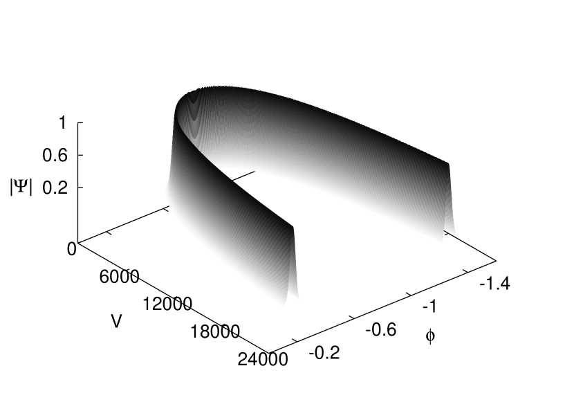
Figure 3: This figure shows the time evolution of absolute value of the wavefunction. For clarity we only show $|\Psi|>10^{-3}$ in the plot. The values of the parameters are $p_{\phi}^{*}=1500\,\hbar\sqrt{G}$, $\sigma=95$ and $\Delta V/V=0.06$. It is clear from the figure that the state remains sharply peaked throughout the evolution.

We will consider two extreme cases: the first corresponds to a sharply peaked state with a large field momentum such that the initial relative volume dispersion is very small compared to unity ($p_{\phi}^{*}=1500\,\sqrt{G}\hbar,\,\sigma=95,\,\Delta V/V\approx 0.06,\,V^{*}\approx 68700\,V_{\rm Pl}$) for which the volume at bounce is $V_{\rm b}=1659.83\,V_{\rm Pl}$, and the second corresponds to a wide state with small field momentum and large initial relative volume dispersion ($p_{\phi}^{*}=20\,\sqrt{G}\hbar,\,\sigma=2.25,\,\Delta V/V\approx 6.44,\,V^{*}=68700\,V_{\rm Pl}$) for which the volume at bounce is $V_{\rm b}=146.22\,V_{\rm Pl}$. As discussed earlier in Sec. 2, here, $\Delta V$ refers to the expectation value of the dispersion in volume, $\langle\Delta V\rangle$. In both of these cases, the initial state is constructed using eq. (31). In this paper, we have considered the evolution of symmetric initial states which have support on $V>0$, and have a very small amplitude near $V=0$. In principle one can consider states which have larger amplitude at or close to $V=0$. However, the part of the state close to $V=0$ contributes very little to the expectation values of the observables, while most of the contribution comes from the larger $V$ domain. It is also noteworthy, that the relative spread in volume $\Delta V/V$ being greater than 1 does not imply that the support of the state extends to negative volume. It is also to be noted that the shape of the wavefunction is symmetric in the variable $\ln(v)$ which leads to high asymmetry around the peak when plotted against $v$ for widely spread states. Due to this, the part of the state that extends to large volume contributes much more to the dispersion in volume $\Delta V$ than the part that extends to smaller volume. Thus, even though the dispersion are larger than 1 for the wide case, the state has support only on positive $V$. The bounce volume is computed after evaluating expectation values of the volume observable using quantum evolution equation in LQC. We consider semi-classical states, corresponding to these two cases, far from bounce and peaked on a classical trajectory on the expanding branch as the initial data. Then we numerically evolve the state backwards using the Chimera scheme. During this evolution, as the energy density grows and the spatial curvature becomes Planckian, the classical trajectory tends to fall into the big bang singularity. In the LQC evolution, the trajectory agrees with the classical one in the low curvature regime and follows it very closely as long as the curvature remains very small compared to Planckian value. During further backward evolution, as the energy density grows closer to the Planck density, the LQC trajectory starts to deviate from the classical trajectory, and unlike the classical theory, the LQC trajectory undergoes a bounce from a finite non-zero volume instead of collapsing into the singularity. This behavior of the LQC trajectories were obtained in Refs. [3, 4, 5] for semi-classical states initially sharply peaked on a classical trajectory, with large $p_{\phi}$.

Figure 3 shows the evolution of a sharply peaked semiclassical state for $p_{\phi}=1500\,\sqrt{G}\hbar$ and $\Delta V/V=0.064$ where the amplitude of the wave-function is plotted with respect to the volume $V$ and emergent time $\phi$. The initial state is constructed as described in Sec. 2. In the numerical simulations, the initial data is provided in the expanding branch and the evolution is carried backwards. It is clear from the figure that the state remains sharply peaked throughout the evolution. The bounce for the state occurs at $V_{\rm b}=1659.83\,V_{\rm Pl}$, when the energy density becomes $\rho\approx 0.408\,\rho_{\rm Pl}$. This value is slightly less than, yet very close to, the upper bound on the energy density, $\rho_{\mathrm{max}}=0.409\,\rho_{\rm Pl}$.

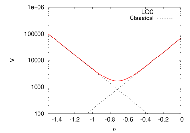
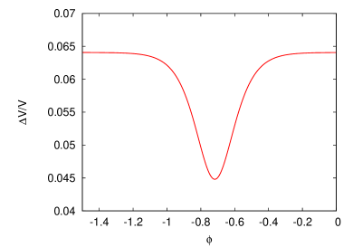
Figure 4: In this figure, the left plot shows the time evolution of the expectation value of the volume and the right plot shows the evolution of the relative volume dispersion of the state at each time, for $p_{\phi}^{*}=1500\,\sqrt{G}\hbar$ and $\Delta V/V=0.064$. The dashed curve in the left plot shows the classical trajectories.

Figure 4 shows the expectation value of the volume and the relative dispersion in the volume as a function of $\phi$ for $p_{\phi}^{*}=1500\,\sqrt{G}\hbar$ and $\Delta V/V=0.064$. The solid (red) curves show the LQC trajectory while the dashed (black) curves mark the two disjoint classical trajectories, one corresponding to the expanding branch and the other to the contracting branch for the same value of $p_{\phi}$. It is straightforward to see from these plots that the LQC trajectory undergoes a non-singular bounce at finite volume. On the other hand, both of the classical trajectories continue to evolve towards the big bang.

As discussed in the previous sections, the numerical evolution of wide states with small $p_{\phi}$ is quite a challenge. Thanks to the Chimera scheme we can now perform such a numerical evolution very efficiently.

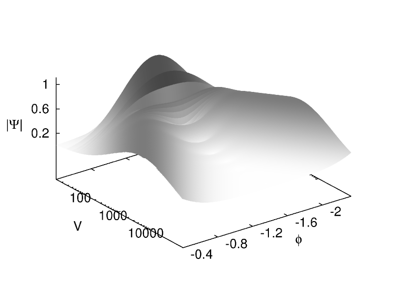
Figure 5: This figure shows the time evolution of the absolute value $|\Psi|$ of a wide state corresponding to parameters $p_{\phi}^{*}=20\,\sqrt{G}\hbar$, $\sigma=2.25$ and $\Delta V/V=6.44$. Far from bounce, both before and after, the state has the form of a Gaussian, whereas it has clear non-Gaussian features in the vicinity of the bounce. Since the state is very spread out in $V$, we have used logscale on $V$-axis.

Fig. 5 shows the evolution of the absolute value of the state $|\Psi|$ as function of $V$ and $\phi$ for the case of $p_{\phi}^{*}=20\,\sqrt{G}\hbar$, $\sigma=2.25$ and $\Delta V/V\approx 6.44$. Note that only a small range of $V$ is shown in the figure. It is clear from the figure that far from the bounce the state has the form of a widely spread Gaussian whereas, in the vicinity of the bounce, the state has non-Gaussian features. The non-Gaussian feature of the state is more apparent in the first panel of Fig. 10, which shows a snapshot of the state at $\phi=-1.35$ close to the bounce. This behavior is very different from the evolution of the sharply peaked state (shown in Fig. 3), where the state remains sharply peaked Gaussian throughout the evolution.

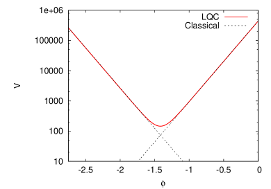
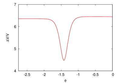
Figure 6: The left plot shows the time evolution of the expectation value of the volume and the right plot shows the evolution of the relative volume dispersion of the state as a function of $\phi$ for $p_{\phi}^{*}=20\,\sqrt{G}\hbar$, $\sigma=2.25$ and $\Delta V/V\approx 6.44$. The dashed curve in the left plot shows the classical trajectories.

Fig. 6 shows the expectation value of $V$ and $\Delta V/V$ with respect to $\phi$, corresponding to the evolution shown in Fig. 5. As can be seen from this figure, the qualitative features of the evolution trajectory of wide states are the same as those of the sharply peaked states. In the low curvature regime, the state follows the classical trajectory while in the Planck regime the corresponding classical trajectory reaches the big bang singularity while the LQC trajectory undergoes non-singular quantum bounce. This happens at a much smaller (but still non zero) volume compared to the sharply peaked state. There is also difference in the value of energy density at which the bounce occurs. In contrast to the previous case, this value turns out to be $\rho=0.009\,\rho_{\rm Pl}$, which is almost two orders of magnitude smaller than the upper bound on the energy density, $\rho_{\mathrm{max}}=0.409\,\rho_{\rm Pl}$.

In table 1 we list representative run times for the $p_{\phi}^{*}=20\,\sqrt{G}\hbar$ and $\Delta V/V\approx 6.44$ case using the Chimera scheme (for both the FD and DG implementations) on a 16 core 2.4 GHz Sandybridge workstation. The first two columns give the grid size ($n_{\mathrm{inner}}$) and run time of evolving only on the inner LQC grid, the next two columns give the outer grid size ($n_{\mathrm{outer}}$) and total run time for the finite difference Chimera scheme and the final two columns give the same information for the DG Chimera scheme. For both cases (FD and DG), $n_{\mathrm{outer}}$ was chosen so that the outer boundary was placed at $v_{\mathrm{outer}}=1.5\times 10^{19}$.

For the FD Chimera scheme, the resolution on the outer WDW grid is chosen to match the resolution of the LQC grid at the interface. In the DG Chimera scheme we use 64th order elements and due to the much higher accuracy, we can use much lower resolution. This is reflected in the much lower values for $n_{\mathrm{outer}}$ for the DG scheme in the table (compared to the FD scheme) and, though the computational cost per grid point is higher in the DG scheme than in the FD scheme, this the main reason for the corresponding much smaller run times. We emphasize that the times listed for the FD and DG Chimera schemes include the time spent on the inner LQC grid.

Table 1: Computational cost for various grid setups. The first two columns lists the number of grid points ($n_{\mathrm{inner}}$) and the time spent on evolution on the inner LQC grid. The next 2 columns lists the number of grid points ($n_{\mathrm{outer}}$) on the outer WDW grid and the total evolution time (on both the inner and outer grid) with the finite difference implementation of the Chimera scheme. The last 2 columns lists the same quantities for evolution with the discontinuous Galerkin Chimera scheme. For both the FD and DG chimera schemes the grid is set up so that the outer boundary is at $v_{\mathrm{outer}}=1.5\times 10^{19}$. The timings are given in total walltime (seconds) when running on 16 cores on a 2.4 GHz Sandybridge workstation.

• LQC grid		Chimera (FD)		Chimera (DG)
  $n_{\mathrm{inner}}$	time (s)	$n_{\mathrm{outer}}$	time (s)	$n_{\mathrm{outer}}$	time (s)
  7,500	38.8	253,953	1117.6	8,125	143.5
  15,000	87.4	497,508	9148.8	15,860	471.3
  30,000	239.3	974,221	40339.0	31,005	1671.0
  60,000	870.0	—	—	60,645	6160.0

The evolution time on the inner LQC grid reveals $n_{\mathrm{inner}}^{2}$ scaling for large $n$, and from this we can estimate that a pure LQC simulation with the outer boundary at $v_{\mathrm{outer}}=1.5\times 10^{19}$ would take $3.4\times 10^{30}$ s $=1\times 10^{23}$ years on this machine (if it had enough memory). For the Chimera scheme the run time is reduced to about half a day for the FD implementation and less than about half an hour for the DG implementation (for the highest resolution listed in the table). For the FD Chimera scheme we did not execute the computational run with $n_{\mathrm{inner}}=60,000$ since it would take a long time. For the DG Chimera scheme the run at $n_{\mathrm{inner}}=30,000$ gives accurate enough results, and a higher resolution is not required for discussion of results. In summary, though most of the computational saving comes from the Chimera scheme, the computational cost was brought down by another order of magnitude through the use of advanced DG methods rather than a straightforward FD implementation.

We now comment on the cost estimates for an implementation of the Chimera scheme to anisotropic models. For simplicity let us consider the case of an LRS Bianchi-I model with a massless scalar field. In this spacetime, two of the scale factors and their time derivatives are equal, while the third scale factor is different. Taking into account that the computational cost of updating one grid point will increase (due to additional evolved variables and derivative terms) and based on the current memory and computational requirements for the 1+1 dimensional code, we can get rough estimates of the requirements for a 2+1 dimensional code. Here, the number of grid points (i.e. memory requirements) would scale as $n^{2}$, as the spatial grid for LRS Bianchi-I spacetime would be two dimensional, and the computational cost as $n^{3}$ (two powers of $n$ from the number of grid points and one power of $n$ from the smaller step size), where $n$ is the number of grid points in one dimension. For the lower resolution case in table 1 with the outer boundary at $v_{\mathrm{outer}}=1.5\times 10^{19}$, we estimate that a 2+1 dimensional code would require of the order 50 Gb of memory and about 20,000 core hours. The next higher resolution would require about 200 Gb of memory and about 160,000 core hours. Assuming that we can write a well scaling code, such simulations could be done comfortably within a day (lowest resolution) or a week (higher resolution) running on 1,000 cores on a typical modern super computer.

5 Tests of the Chimera scheme

In the previous section, we have discussed that the DG method is far more efficient and computationally inexpensive compared to the FD method. For this reason, we will focus on the discussion of the DG method. We now describe the concept of convergence for the Chimera scheme for the DG method, and present detailed tests. There are two major concerns regarding the accuracy of the numerical results. The first is the effect of the interface between the LQC and WDW grid and the second is due to the initial data being chosen as a WDW state with an additional phase (eq. (31)). With regard to the first issue, we have to choose the location of $v_{\mathrm{interface}}$ large enough such that the WDW equations are a good approximation to the LQC equations. We can control the errors from the interface by performing runs with different values for $v_{\mathrm{interface}}$ and compare the results. As the resolution on the WDW grid is chosen to match the resolution on the LQC grid in $v$-space, increasing $v_{\mathrm{interface}}$ automatically results in higher resolution (in $x$) on the WDW grid. Thus, increasing $v_{\mathrm{interface}}$ results in higher accuracy due to two different factors. The WDW equations are better approximations to the LQC equations, and the WDW equations are solved with higher numerical resolution. With regard to the second issue, we are interested in setting up a simulation where the state starts to travel inwards (towards smaller volume) as the evolution proceeds. We will refer to this as an ingoing mode. Similarly we refer to a mode that initially travels outwards (towards larger volume) as an outgoing mode. Initial data constructed as a pure ingoing WDW state will have a small (depending on where the state is peaked and how wide it is) outgoing LQC mode. We can reduce the amplitude of this outgoing mode by starting the simulation at a larger value of $\phi_{\mathrm{o}}$. However, we demonstrate that, if the state is setup on the WDW grid, the interface between the LQC and WDW grids also helps by acting as a filter that reflects the outgoing LQC mode.

5.1 Convergence for a sharply peaked state

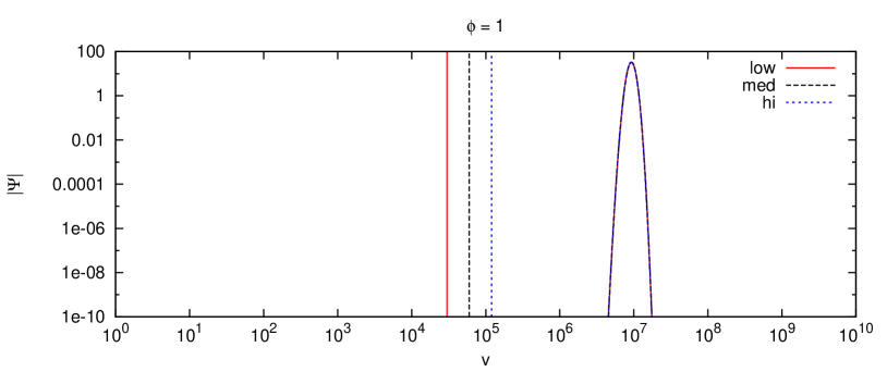
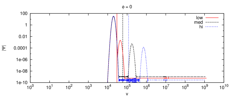
Figure 7: Log-log plots of the absolute value of the state as a function of the volume variable $v$. Here snapshots of the evolution of a sharply peaked state with $p_{\phi}^{*}=1500\,\sqrt{G}\hbar$ and $\Delta V/V=0.064$ at $\phi=1$ (upper panel) and $\phi=0$ (lower panel). The solid (red), dashed (black) and dotted (blue) curves are for the low ($v_{\mathrm{interface}}=30,000$), medium ($v_{\mathrm{interface}}=60,000$) and high ($v_{\mathrm{interface}}=120,000$) resolution runs, respectively. For clarity the thinner vertical lines shows the position of $v_{\mathrm{interface}}$ for the three cases.

.

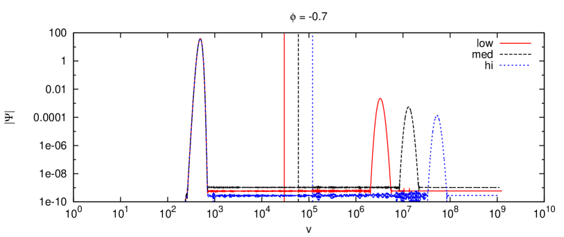
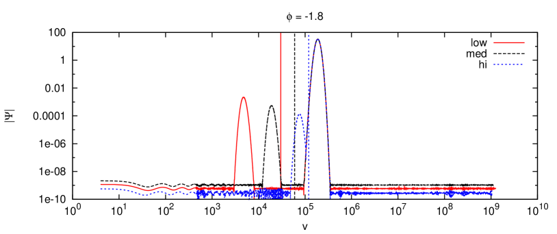
Figure 8: Log-log plots of the absolute value of the state as a function of the volume variable $v$. Here snapshots of the evolution of a sharply peaked state with $p_{\phi}^{*}=1500\,\sqrt{G}\hbar$ and $\Delta V/V=0.064$ at $\phi=-0.7$ (upper panel) and $\phi=-1.8$ (lower panel). The solid (red), dashed (black) and dotted (blue) curves are for the low ($v_{\mathrm{interface}}=30,000$), medium ($v_{\mathrm{interface}}=60,000$) and high ($v_{\mathrm{interface}}=120,000$) resolution runs, respectively. For clarity the thinner vertical lines shows the position of $v_{\mathrm{interface}}$ for the three cases.

.

In figures 7 and 8 we show four snapshots of the evolution of a sharply peaked state with $p_{\phi}^{*}=1500\,\sqrt{G}\hbar$ and $\Delta V/V=0.064$ starting at $\phi=1$. The upper panel in Fig. 7 shows the initial state at $\phi=1$ while the lower panel shows the state at $\phi=0$ when it has just passed through the interfaces, denoted by vertical lines. We consider three different resolutions, corresponding to three different locations of the interface: the solid (red), dashed (black) and dotted (blue) curves correspond to the low, medium and high resolution respectively. It is clear from the figures that as the state passes through an interface, a part of the state is reflected from it. Properties of the reflected parts depend on the location of the interface. For example, in the higher resolution case, since the interface is further out, the reflection occurs earlier and the reflected part of the state has propagated to a larger volume than the low and medium resolution cases. Moreover, the amplitude of the reflected part of the state converges to zero to second order in $v_{\mathrm{interface}}$. That is, when $v_{\mathrm{interface}}$ doubles, the amplitude decreases by a factor of four. The almost flat but noisy features trailing the state at around the $10^{-9}$ level (different at different resolutions) is caused by a combination of roundoff and truncation errors. In Fig. 8, the upper panel shows the state at $\phi=-0.7$ close to the bounce which occurs at $\phi_{\mathrm{b}}=-0.71744$ at $V_{\mathrm{b}}=1659.83V_{\mathrm{Pl}}$. In this figure, the reflected part of the waves have propagated further to the right (towards larger $v$). The lower panel of Fig. 8 shows the state at $\phi=-1.8$ just after it has crossed the interface one more time. Again there is a reflected part of the state, now propagating to the left (towards smaller $v$). The amplitude is again second order convergent in $v_{\mathrm{interface}}$ and since the state has to propagate to larger $v$ before hitting the interface in the high resolution case, the reflected part of the state is delayed, as compared to the lower resolution cases. This allows a larger time interval between the two reflections (first before bounce and the second afterwards) at the interface, in the case of high resolution. The first reflection is caused by the fact that the initial state is set up as a purely ingoing WDW state. It evolves cleanly until it hits the interface. As this purely ingoing WDW state is not a purely ingoing LQC state, it contains a small outgoing component. This component can not be propagated inwards and is reflected. In this sense the interface acts as a filter that ensures that the state on the LQC grid is purely ingoing. If the initial state was set up completely contained within the LQC grid, we would see a small part of the state immediately starting to move outwards. Note that the outer boundary in this simulation was placed at $v\approx 10^{9}$, allowing us to set up the state at $\phi=1$ where it is peaked at $v\approx 10^{7}$. This would have been prohibitively expensive using only an LQC grid.

5.2 Convergence for a wide state

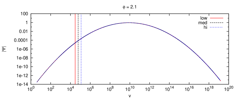
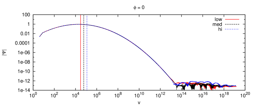
Figure 9: Log-log plots of the absolute value of the state as a function of the volume variable $v$. Here snapshots of the evolution of a very wide state with $p_{\phi}^{*}=20\,\sqrt{G}\hbar$ and $\Delta V/V\approx 6.44$ at $\phi=2.1$ (upper panel) and $\phi=0$ (lower panel). The solid (red), dashed (black) and dotted (blue) curves are for the low ($v_{\mathrm{interface}}=30,000$), medium ($v_{\mathrm{interface}}=60,000$) and high ($v_{\mathrm{interface}}=120,000$) resolution runs, respectively. For clarity the thinner vertical lines shows the position of $v_{\mathrm{interface}}$ for the three cases.

.

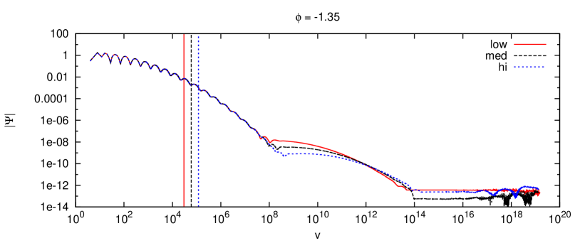
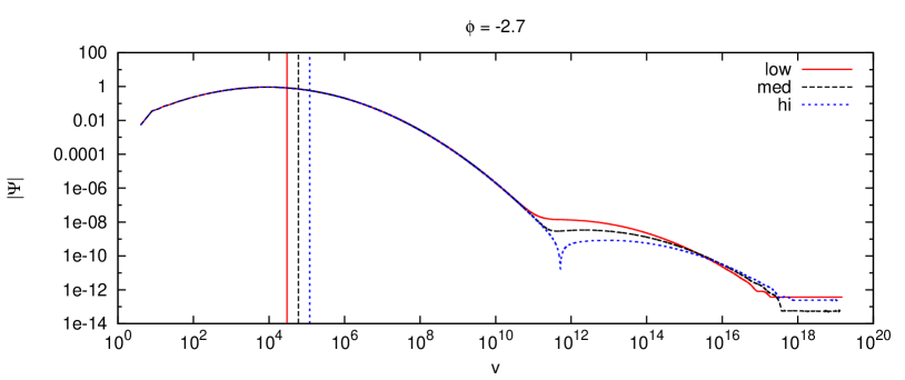
Figure 10: Log-log plots of the absolute value of the state as a function of the volume variable $v$. Here snapshots of the evolution of a very wide state with $p_{\phi}^{*}=20\,\sqrt{G}\hbar$ and $\Delta V/V\approx 6.44$ at $\phi=-1.35$ (upper panel) and $\phi=-2.7$ (lower panel). The solid (red), dashed (black) and dotted (blue) curves are for the low ($v_{\mathrm{interface}}=30,000$), medium ($v_{\mathrm{interface}}=60,000$) and high ($v_{\mathrm{interface}}=120,000$) resolution runs, respectively. For clarity the thinner vertical lines shows the position of $v_{\mathrm{interface}}$ for the three cases.

.

In figures 9 and 10 we similarly show four snapshots of the evolution of a very wide state with $p_{\phi}^{*}=20\,\sqrt{G}\hbar$ and $\Delta V/V\approx 6.44$ starting at $\phi=2$. The upper panel in Fig. 9 shows the initial state at $\phi=2$. As in Fig. 7 and Fig. 8, the vertical lines indicate the position of the interface boundary for each of the three different resolutions. Note that the state is so wide that we need to place the outer boundary at $v=10^{19}$ in order to contain the state within the numerical domain, and that it has non-zero amplitude on the inner LQC domain. This means that there is a non-zero outgoing LQC mode from the beginning of the simulation. However, the amplitude is small and does not affect the measurement of the expectation value of $V$ and its spread $\Delta V$. The lower panel shows the state at $\phi=0$. In the outer part of the grid the numerical solution is dominated by roundoff errors, while in the inner part of the grid part of the state has already started to bounce. The upper panel in Fig. 10 shows the state at $\phi=-1.35$ close to the bounce which occurs at $\phi_{\mathrm{b}}=-1.4167$ at $V_{\mathrm{b}}=146.219V_{\mathrm{Pl}}$. For $v>10^{8}$ it is possible to see the part of the state that has been reflected off the interface boundary. The amplitude of the reflection is much smaller compared to the case of the narrow state. In this case the reflected amplitude is about $10^{8}$ times smaller than the amplitude of the state. As before, the amplitude converges to zero at second order with the interface position $v_{\mathrm{interface}}$. The lower panel shows the state at $\phi=-2.7$ well after the peak has bounced. At this point the shoulder of the reflection propagates cleanly towards large $v$ ahead of the bouncing state.

It is clear from Fig. 10 that, unlike the case of sharply peaked state whose shape always remains a smooth and sharply peaked Gaussian in the evolution, the wide state with $p_{\phi}^{*}=20\,\sqrt{G}\hbar$ and $\Delta V/V\approx 6.44$ shows non-Gaussian features at $\phi\approx-1.35$ near the bounce. This behavior, as discussed in section 4, can also be seen in figure 5 which shows a 3D evolution of the absolute value of the state, $|\Psi|$ with respect to $V$ and $\phi$. However, as shown in the second panels of Fig. 9 and Fig. 10, the shape of the wide state far from bounce, both before (at $\phi=0$) and after the bounce (at $\phi=-2.7$), is a smooth Gaussian. Hence, far from the bounce the shape of the state is smooth for both the sharply peaked and widely spread states, while there are differences in the qualitative features of the shape of the wide states close to the bounce.

5.3 Convergence of $\Delta V/V$

When calculating the expectation value of the volume $V$ of the state and its corresponding spread $\Delta V$, as given in eq. (26) and eq. (27), we need to integrate over the state. As the integrand used to compute the expectation value of $v^{2}$ contains an extra factor of $v$, it is clear from Fig. 9 that we would get contributions from the roundoff error (noise at the $10^{-13}$ level contributes significantly when multiplied by $10^{19}$) if the integration is extended all the way to the outer boundary. For this reason we need to choose a volume $v_{\mathrm{int}}$ at which the integration is stopped. On one hand, if we choose $v_{\mathrm{int}}$ to be too small, we may not have the whole state contained in the integration domain. On the other hand, if we choose it too large we may get spurious contributions from the roundoff error noise or from the reflected part of the state. In fact, in many cases, it is impossible to choose a value for $v_{\mathrm{int}}$ that is satisfactory for the whole simulation. We illustrate this in figures 11, 12 and 13 for the extreme case of $p_{\phi}^{*}=20\,\sqrt{G}\hbar$ and $\Delta V/V\approx 6.44$ at low, medium and high resolutions respectively.

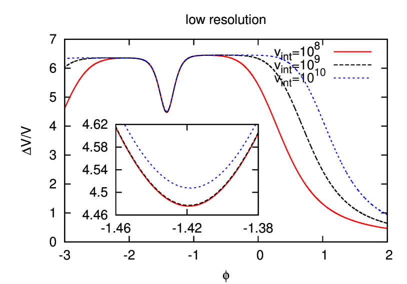
Figure 11: $\Delta V/V$ for 3 different integration radii: $v_{\mathrm{int}}=10^{8}$ (solid/red line), $v_{\mathrm{int}}=10^{9}$ (dashed/green line) and $v_{\mathrm{int}}=10^{10}$ (dotted/blue line) for the case $p_{\phi}^{*}=20\,\sqrt{G}\hbar$ and $\Delta V/V\approx 6.44$ at low resolution $v_{\mathrm{interface}}=30,000$. the inset shows in detail what happens near the bounce.

.

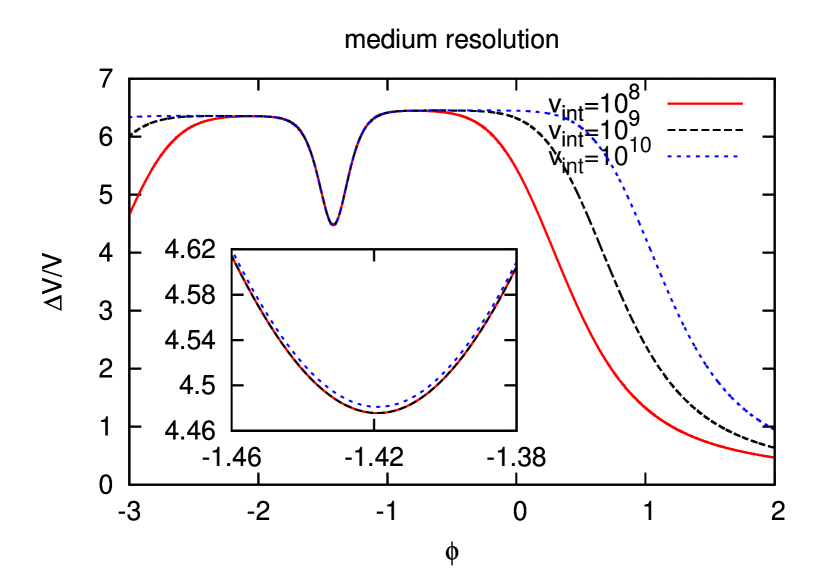
Figure 12: $\Delta V/V$ for 3 different integration domains: $v_{\mathrm{int}}=10^{8}$ (solid/red line), $v_{\mathrm{int}}=10^{9}$ (dashed/green line) and $v_{\mathrm{int}}=10^{10}$ (dotted/blue line) for the case $p_{\phi}^{*}=20\,\sqrt{G}\hbar$ and $\Delta V/V\approx 6.44$ at medium resolution $v_{\mathrm{interface}}=60,000$. The inset shows in detail what happens near the bounce.

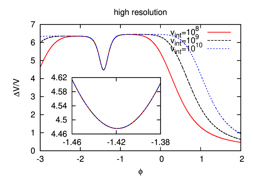
Figure 13: $\Delta V/V$ for 3 different integration domains: $v_{\mathrm{int}}=10^{8}$ (solid/red line), $v_{\mathrm{int}}=10^{9}$ (dashed/green line) and $v_{\mathrm{int}}=10^{10}$ (dotted/blue line) for the case $p_{\phi}^{*}=20\,\sqrt{G}\hbar$ and $\Delta V/V\approx 6.44$ at high resolution $v_{\mathrm{interface}}=120,000$. The inset shows in detail what happens near the bounce.

.

In all cases, the plots show the calculated value of $\Delta V/V$ as function of $\phi$ using three different values of $v_{\mathrm{int}}$. The solid (red) curve is for $v_{\mathrm{int}}=10^{8}$, the dashed (green) curve is for $v_{\mathrm{int}}=10^{9}$ and the dotted (blue) curve is for $v_{\mathrm{int}}=10^{10}$. At late times, when the state is peaked at large volume (the WDW regime), $\Delta V/V$ should be constant. However, in this regime the state is not completely contained within the integration volume and we get different values for $\Delta V/V$ for the three different values of $v_{\mathrm{int}}$. As the state contracts further (as $\phi$ decreases) it becomes small enough that first $v_{\mathrm{int}}=10^{10}$, then $v_{\mathrm{int}}=10^{9}$ and finally $v_{\mathrm{int}}=10^{8}$ is large enough to contain the state. After this we get good agreement between the calculations of $\Delta V/V$ using the three different values of $v_{\mathrm{int}}$ through the bounce (at $\phi=-1.42$ in this case) and for some time afterwards until the state expands and become large enough that it no longer is contained within the integration volume. A close up of the near bounce region at low resolution (see the inset in Fig. 11), however, reveals some small differences. A small difference is visible between the $v_{\mathrm{int}}=10^{8}$ and $v_{\mathrm{int}}=10^{9}$ curves while the $v_{\mathrm{int}}=10^{10}$ curve shows a clear deviation from the other curves. These are caused by the reflected part of the state of the interface between the inner LQC grid and the outer WDW grid seen in Fig. 9. However, as the interface between the two grids are moved out (and the resolution is increased), the amplitude of the reflection decreases. Thus at the medium resolution (see the inset in Fig. 12), the $v_{\mathrm{int}}=10^{8}$ and $v_{\mathrm{int}}=10^{9}$ curves agree very nicely, while the deviation of the $v_{\mathrm{int}}=10^{10}$ curve has decreased significantly compared to the low resolution case. Finally in the high resolution case (see the inset in Fig. 13) all three curves agree nicely all the way through the bounce. Thus we conclude that the interface between the grids is far enough out in the “classical” region that any artifacts introduced by the Chimera scheme do not affect the results. For different initial data parameters, the optimal choice of $v_{\mathrm{int}}$ will be different, so in each case we have to perform simulations at different resolutions and examine the plots of $\Delta V/V$ for different $v_{\mathrm{int}}$. For the sharply peaked state shown in Fig. 7 and Fig. 8, for example, we find that $v_{\mathrm{int}}=10^{5}$ is sufficient. Even though the roundoff noise is in the integration volume at the bounce, it is at a sufficiently low level that it does not adversely affect the value of $\Delta V/V$. Also the reflected wave in that case (of much larger amplitude than the really wide state) leaves the integration volume as early as $\phi\approx 0$ in the high resolution case.

As the integrand for the expectation value of $v$ in eq. (26) only contains one factor of $v$, the errors for the expectation value are much smaller than for the dispersion. Thus convergence of $\Delta V/V$ implies convergence of the expectation value of $V$ as well.

5.4 Comparison with pure LQC evolution

As a final test, we want to compare the Chimera scheme with a pure LQC evolution, i.e. with the outer WDW grid turned off. As the wide state requires the outer boundaries to be placed at $v=1.5\times 10^{19}$, it is unfeasible to make a comparison in this case. So for the comparison we use the sharply peaked state shown in figures 7 and 8. Those simulations where started at $\phi_{o}=1$ where the state is peaked at $v\approx 10^{7}$, requiring the outer boundary to be located at at least $v_{\mathrm{outer}}=2\times 10^{7}$. Using the results of runs in Table 1, the estimated time to complete such a simulation turns out to be approximately 70 days on a workstation. Thus, this simulation is too expensive to do with a pure LQC grid. Therefore, to do the comparison we take the following strategy. We perform three pure LQC simulations with different starting times $\phi_{o}=(0,0.1,0.2)$ with $v_{\mathrm{outer}}=240,000$ and compare with the Chimera runs. In these three cases the state is initially peaked at $v=20,000$, $37,000$ and $70,000$, respectively. In all these cases, states are so sufficiently far inside the outer boundary, that we avoid any outer boundary problems.

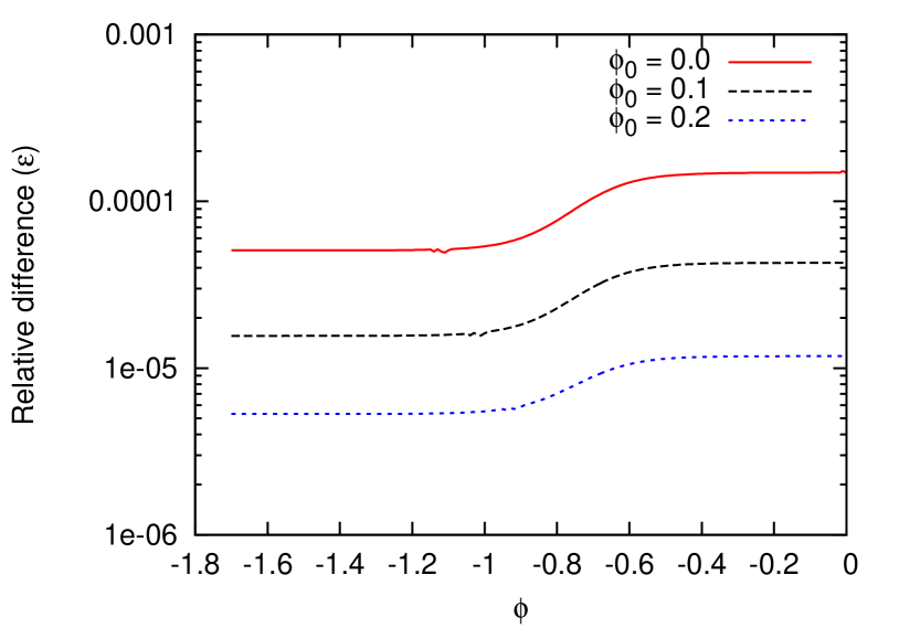
Figure 14: The relative difference $\varepsilon=|\langle\hat{v}\rangle_{\mathrm{LQC}}-\langle\hat{v}\rangle_{\mathrm{Chimera}}|/\langle\hat{v}\rangle_{\mathrm{Chimera}}$ for different starting $\phi_{0}$ as function of $\phi$ for the sharply peaked state $p_{\phi}^{*}=1500\,\sqrt{G}\hbar$ and $\Delta V/V=0.064$. The solid (red) curve is for $\phi_{0}=0$, the dashed (black) curve is for $\phi_{0}=0.1$ and the dotted (blue) curve is for $\phi_{0}=0.2$

.

In Fig. 14 we plot the relative difference in the expectation value of $v$ between the pure LQC simulations and the Chimera simulation as function of $\phi$ for the three different starting times. For $\phi_{o}=0$ the relative difference is of order $10^{-4}$. This difference is due to the fact that the initial state is setup as a solution to the WDW equations and therefore is not a pure ingoing mode for the LQC equations. We use the term ingoing in the same sense here as we did in the beginning of Sec. 5. As $\phi_{o}$ increases, the state is initially peaked at larger $v$ and the WDW initial state is a better approximation to the pure ingoing LQC state. Therefore we see the relative difference decreases for larger values of $\phi_{o}$, and for $\phi_{o}=0.2$ the difference is of order $10^{-5}$. In fact the decrease in relative difference shown in the figure is consistent with second order convergence in the starting location (in $v$) of the peak of the state and is also consistent with the second order convergence in the amplitude of the reflected part of the state off the interface boundary when the Chimera scheme is used. This again shows the advantage of being able to use a large domain, allowing us to setup the initial data peaked at a large enough volume that the errors made in constructing the state as a WDW state is negligible.

6 Discussion

In this article we have presented an efficient numerical technique to study the evolution of states in LQC. Previously, numerical simulations in isotropic LQC were performed with a massless scalar field as the matter source with a large value of the field momentum for sharply peaked states. All such simulations show the existence of a quantum bounce at an energy density which is very close to the maximum value of the energy density, $\rho_{\rm max}\approx 0.41\rho_{\mathrm{Planck}}$, computed from an exactly solvable model (with lapse $N=V$) [9]. Though the robustness of the bounce has been verified in various models, it was so far not observed for states with small field momentum and with very wide spreads, or for non-Gaussian states. Such states can be thought of as corresponding to universes which are more ‘quantum’ compared to the states previously considered in numerical simulations in LQC. Using the results of [9], it has recently been suggested that a certain class of squeezed states may lead to a quantum bounce [11] at a much lower energy density. Further, a detailed study of states which have wide spread, small field momentum and non-Guassian features is critical in order to understand the validity of the effective spacetime description in LQC [8]. However, testing the robustness of new physics in LQC for such kinds of states using numerical simulation is a computationally challenging task, which is extremely difficult to perform with the existing techniques. These difficulties are further aggravated in the case of anisotropic models due to the increased number of spatial dimensions (leading to much larger computational domains). In addition, certain non-trivial properties of the anisotropic quantum difference equation, which are absent in the isotropic model, complicates the implementation of numerical codes.

In order to tackle these computational challenges, we have proposed and implemented a hybrid numerical technique, Chimera, which uses a combination of LQC and WDW computational grids. This scheme is based on a crucial property of the quantum Hamiltonian constraint in LQC – that it is approximated extremely well by the WDW Hamiltonian constraint at large volumes. The inner grid, corresponding to a lower volume range, is a uniform discrete grid based on the discreteness given by LQC. It is taken to be reasonably large such that all the non-trivial features of the physics of LQC is contained within this domain, and there is little difference between the LQC and WDW evolution at the outer boundary of the inner grid. The outer grid, on the other hand, is a grid with a continuum limit on which we solve the WDW equation. Here we have utilized the fact that the isotropic LQC difference equation can be approximated by a second order finite differencing approximation to the WDW equation in the large volume limit. Using advanced techniques for solving PDE’s, we can explore efficient ways to evolve the state on the outer grid. We studied two such methods: a finite difference implementation, and a discontinuous Galerkin method. We find that discontinuous Galerkin method turns out to be extremely efficient. Evolutions with widely spread states which would have taken $10^{23}$ years can now be performed in a few hours on a modern workstation. We further performed various convergence tests with the discontinuous Galerkin method, verified crucial properties of the evolutions of sharply and widely peaked states and studied the behavior of the relative fluctuations in comparison with pure LQC evolutions. Our analysis shows that the Chimera scheme proves to be very advantageous both in terms of the accuracy of the results and the computational cost. More importantly, with the scheme presented here, we are able to perform simulations with a very wide variety of states. Using the run time estimates for isotropic models, the Chimera scheme also promises a very significant reduction in computational costs for the anisotropic models. The computational costs in these models scales as $n^{3}$ for LRS Bianchi-I spacetimes, and as $n^{4}$ for Bianchi-I models with a massless scalar field, making them practically very difficult to study even with supercomputers. Our estimates show that using the Chimera scheme, many of these simulations can be performed in less than a week on current super computers. Thus, the Chimera scheme promises to be an important tool to explore so far unknown regimes of LQC in various models.

The current article is the first in a series of papers focused towards building an efficient and portable numerical infrastructure for the simulations of various cosmological models in the paradigm of LQC. Here, we have only provided the details of the numerical properties of the scheme using sharply peaked and widely spread Gaussian states for the spatially flat isotropic model (with lapse $N=1$). Our results can then be viewed as a generalization of earlier results in [5] where simulations were carried out for sharply peaked states for large $p_{\phi}$. In an upcoming paper, we will use the Chimera scheme to understand the validity of the effective spacetime description in detail for widely spread states by exploring regions much closer to Planck volume than considered so far in the literature [30]. As discussed in the paper, our scheme is not limited to simulations of Gaussian states in isotropic loop quantum cosmology. We have used the Chimera scheme to perform numerical evolutions of various other non-Gaussian states, such as squeezed states and other states with nontrivial features [28]. Going beyond the massless scalar models, the Chimera scheme has also been used to perform numerical simulations in LQC with negative potentials giving rise to cyclic models of the universe [29]. In ongoing work, we are implementing the Chimera method to study the numerical evolution of models with more degrees of freedom using high performance computing resources.

Appendix A Discontinuous Galerkin methods

In this appendix we describe the main ideas behind Discontinuous Galerkin (DG) methods. The notation and discussion is borrowed heavily from [37] which we recommend for further reading. To understand DG methods, it is easiest to look at the simplest possible PDE, i.e. the 1-d scalar advection equation

$$\frac{\partial u}{\partial t}+\frac{\partial f(u)}{\partial x}=0,\mbox{\hskip 20.00003pt}x\in[L,R]=\Omega,$$ (52)

where $f(u)=au$ and $a$ is a constant. The numerical domain $\Omega$ is approximated by $K$ non-overlapping elements ${\cal D}^{k}$

$$\Omega\simeq\Omega_{h}=\bigcup_{k}^{K}{\cal D}^{k},$$ (53)

where $x\in[x_{l}^{k},x_{r}^{k}]={\cal D}^{k}$, and where $x_{r}^{k}=x_{l}^{k+1}$ (see Fig. 15).

Figure 15: This figure illustrates the way the numerical domain $\Omega=[L,R]$ is split into 4 non-overlapping 5th order elements ${\cal D}^{1},\ldots,{\cal D}^{4}$. The black dots above (for ${\cal D}^{1}$ and ${\cal D}^{3}$) and below (for ${\cal D}^{2}$ and ${\cal D}^{4}$) the coordinate line shows the location of the 6 nodes inside each 5th order element. Notice that the nodes are not distributed evenly inside the element and that the boundary nodes on neighboring elements have the same coordinates.

Within each element, the local solution is approximated as a polynomial of order $N=N_{p}-1$:

$$x\in{\cal D}^{k}:u_{h}^{k}(x,t)=\sum_{n=1}^{N_{p}}\hat{u}_{n}^{k}(t)\psi_{n}(x)=\sum_{i=1}^{N_{p}}u_{h}^{k}(x_{i}^{k},t)\ell_{i}^{k}(x).$$ (54)

Here $u_{h}^{k}(x,t)$ denote the numerical approximation to the solution $u(x,t)$ within element $k$. In the first sum the numerical approximation is expressed in terms of an expansion in a polynomial basis, where $\psi_{n}(x)$ are the basis functions and $\hat{u}_{n}^{k}$ are the coefficients. This is called the modal form. In the second sum the numerical approximation is expressed in terms of a sum of interpolating polynomials. Here a set of $N_{p}$ distinct nodes $x_{i}^{k}$ (see Fig. 15) are defined within each element and the interpolating polynomials $\ell_{i}^{k}(x)$ satisfies $\ell_{i}^{k}(x_{j}^{k})=\delta_{ij}$. This is called the nodal form. In the following, we will only consider the nodal form. The global solution is then approximated by the piecewise $N$-th order polynomial

$$u(x,t)\simeq u_{h}(x,t)=\bigoplus_{k=1}^{K}u_{h}^{k}(x,t),$$ (55)

i.e. the direct sum of the $K$ local polynomial solutions $u_{h}^{k}(x,t)$. Note that the global solution is multi-valued at element boundaries.

We finally define the numerical residual

$${\cal R}_{h}(x,t)=\frac{\partial u_{h}}{\partial t}+\frac{\partial f(u_{h})}{\partial x}$$ (56)

by inserting the numerical approximation to the solution $u_{h}(x,t)$ into the continuum eq. (52). Since the numerical solution has a finite number of degree of freedom, the residual ${\cal R}_{h}(x,t)$ can not be zero everywhere (unless the continuum solution itself is an $N$th order polynomial). To quantify how small the residual is, it is natural to use a suitable defined inner product and norm. Within element $k$, we define the local inner product and norm as

$$\left(u,v\right)_{{\cal D}^{k}}=\int_{{\cal D}^{k}}uv\,dx,\mbox{\hskip 10.00002pt}\|u\|_{{\cal D}^{k}}^{k}=\left(u,u\right)_{{\cal D}^{k}},$$ (57)

and with this we define the global inner product and norm as

$$(u,v)_{\Omega,h}=\sum_{k}^{K}\left(u,v\right)_{{\cal D}^{k}},\mbox{\hskip 10.00002pt}\|u\|_{\Omega,h}=(u,u)_{\Omega,h}.$$ (58)

In a Galerkin method the choice is then made to require that the residual is orthogonal to all the basis functions in which the numerical solution is expanded, i.e.

$$\left({\cal R}_{h},\psi_{n}\right)_{{\cal D}^{k}}=\int_{{\cal D}^{k}}{\cal R}_{h}(x,t)\psi_{n}(x)\,dx=0,\mbox{\hskip 10.00002pt}1\leq n\leq N_{p}.$$ (59)

This is a local statement on each element and does not connect the solution between neighboring elements. Since the interpolating polynomials can be expanded uniquely in the basis functions an equivalent set of conditions can be written in nodal form

$$\left({\cal R}_{h},\ell_{i}^{k}\right)_{{\cal D}^{k}}=\int_{{\cal D}^{k}}{\cal R}_{h}(x,t)\ell_{i}^{k}(x)\,dx=0,\mbox{\hskip 10.00002pt}1\leq i\leq N_{p}.$$ (60)

Equation (60) results in $N_{p}$ equations for the $N_{p}$ unknowns $u_{h}^{k}(x_{i}^{k},t)$ within each element. Using integration by parts we find

$$\left({\cal R}_{h},\ell_{i}^{k}\right)_{{\cal D}^{k}}=\int_{{\cal D}^{k}}\left(\frac{\partial u_{h}^{k}}{\partial t}-f(u_{h}^{k})\frac{\partial\ell_{i}^{k}}{\partial x}\right)\,dx+\left[f(u_{h}^{k})\ell_{i}^{k}\right]_{x_{l}^{k}}^{x_{r}^{k}},$$ (61)

where the surface term can be used to glue the solution in neighboring elements together. This can be achieved by replacing $f(u_{h}^{k})$ in the boundary term in eq. (61) by a numerical flux $f^{*}$ that depends on the solution on both sides of the boundary. This leads to the so called weak form of the equations

$$\int_{{\cal D}^{k}}\left(\frac{\partial u_{h}^{k}}{\partial t}-f(u_{h}^{k})\frac{\partial\ell_{i}^{k}}{\partial x}\right)\,dx=-\left[f^{*}\ell_{i}^{k}\right]_{x_{l}^{k}}^{x_{r}^{k}},\mbox{\hskip 10.00002pt}1\leq i\leq N_{p},$$ (62)

where $f^{*}$ at the right boundary of element $k$ is a suitable function of both $u_{h}^{k}(x_{r}^{k})$ (from element $k$ and $u_{h}^{k+1}(x_{l}^{k+1})$ (from element $k+1$). Using integration by parts on the weak form of the equations we obtain the strong form of the equations

$$\int_{{\cal D}^{k}}{\cal R}_{h}(x,t)\ell_{i}^{k}(x)\,dx=\left[(f(u_{h}^{k})-f^{*})\ell_{i}^{k}\right]_{x_{l}^{k}}^{x_{r}^{k}},\mbox{\hskip 10.00002pt}1\leq i\leq N_{p}.$$ (63)

It turns out that the choice of $f^{*}$ is not unique. Often it can be tailored to be optimal for the set of equations being considered. An often used expression for the numerical flux that works well in many cases is the Lax-Friedrichs flux along the normal $\hat{n}$

$$f^{*}=f^{\mathrm{LF}}(a,b)=\frac{f(a)+f(b)}{2}+\frac{C}{2}\hat{n}(a-b),$$ (64)

where $(a,b)$ represents internal and external values, respectively and

$$0\leq C\leq\max\left|\frac{\partial f}{\partial u}\right|$$ (65)

where the maximum has to be taken over all nodes in the element. For the simple advection equation it can be proven that this choice of flux leads to a stable scheme. For $C=0$ we have a symmetric flux that just depends on the average flux on either side of the element boundary (hence the name). For positive values of $C$ the jump in the solution across the element boundary is taken into account. For $f(u)=au$ and $C=|a|$ the Lax-Friedrich flux becomes an upwinding flux in the sense that information is used only in the direction in which it is traveling. Inserting now the expansion of the numerical approximation in interpolating polynomials from eq. (54) into the strong form of the equations eq. (63) and rewriting in matrix form we find

$${\cal M}^{k}\frac{d}{dt}\bm{u}_{h}^{k}+{\cal S}^{k}a\bm{u}_{h}^{k}=\left[(au_{h}^{k}-(au_{h})^{*})\bm{\ell}^{k}(x)\right]_{x_{r}^{k}}^{x_{l}^{k}},$$ (66)

where we have defined the solution vector $\bm{u}_{h}^{k}$ and interpolating polynomial vector as

$$\bm{u}_{h}^{k}=\left[u_{h}^{k}(x_{1},t),\ldots,u_{h}^{k}(x_{N_{p}},t)\right],\mbox{\hskip 20.00003pt}\bm{\ell}^{k}(x)=\left[\ell_{1}^{k}(x),\ldots,\ell_{N_{p}}^{k}(x)\right]$$ (67)

and the mass matrix ${\cal M}^{k}$ and stiffness matrix ${\cal S}^{k}$ are given by

$${\cal M}_{ij}^{k}=\left(\ell_{i}^{k},\ell_{j}^{k}\right)_{{\cal D}^{k}},\mbox{\hskip 20.00003pt}{\cal S}_{ij}^{k}=\left(\ell_{i}^{k},\frac{d\ell_{j}^{k}}{dx}\right)_{{\cal D}^{k}}.$$ (68)

Multiplying through with the inverse of the mass matrix $({\cal M}^{k})^{-1}$ and defining the differentiation matrix ${\cal D}_{r}^{k}=({\cal M}^{k})^{-1}{\cal S}^{k}$ we find

$$\frac{d}{dt}\bm{u}_{h}^{k}=-a{\cal D}_{r}^{k}\bm{u}_{h}^{k}+\left({\cal M}^{k}\right)^{-1}\left[\bm{\ell}^{k}(x)(au_{h}^{k}-(au_{h})^{*})\right]_{x_{r}^{k}}^{x_{l}^{k}}.$$ (69)

If we now form the 2-element boundary vector $\bm{v}=[v_{1},v_{2}]^{T}$ where $v_{1}=(au_{h}^{k}-(au_{h})^{*})|_{x_{r}^{k}}$ and $v_{2}=(au_{h}^{k}-(au_{h})^{*})|_{x_{l}^{k}}$ (i.e. $\bm{v}$ contains the boundary terms of the element which are coupled to the neighboring elements through the numerical Lax-Friedrich flux $(au_{h})^{*}$) and use the properties that $\bm{\ell}^{k}(x_{r}^{k})=\delta_{i1}$ and $\bm{\ell}^{k}(x_{l}^{k})=\delta_{iN_{p}}$ to introduce the $N_{p}\times 2$ vector

$$\bm{b}=\left(\begin{array}[]{cc}1&0\\ 0&0\\ \vdots&\vdots\\ 0&1\end{array}\right)$$ (70)

we can rewrite the boundary term and obtain

$$\frac{d}{dt}\bm{u}_{h}^{k}=-a{\cal D}_{r}^{k}\bm{u}_{h}^{k}+{\cal L}^{k}\bm{v}$$ (71)

where the lift matrix ${\cal L}^{k}$ is defined as

$${\cal L}^{k}=({\cal M}^{k})^{-1}\bm{b}.$$ (72)

Given the differentiation matrix and the lift matrix, the RHS evaluation in the DG scheme consists of construction of the boundary matrix (using e.g. the Lax-Friedrich flux) and then performing matrix-vector multiplications to calculate the spatial derivative and the boundary correction.

The above discussion provides a brief summary of the general idea behind the DG method. There are still several technical details that needs to be addressed before it can be turned into a working numerical algorithm. For example, we have not described how the nodal points inside the elements are chosen (there is a reason the nodes are unequally spaced) and we have left out any discussion of how to numerically construct the differentiation and lift matrix. For further details, we refer the reader to [37].

References

References

- [1] Abhay Ashtekar and Parampreet Singh, Loop Quantum Cosmology: A Status Report, Class. Quant. Grav., 28:213001, 2011.
- [2] Parampreet Singh, Are loop quantum cosmos never singular? Class. Quant. Grav., 26:125005, 2009.
- [3] Abhay Ashtekar, Tomasz Pawlowski, and Parampreet Singh, Quantum nature of the big bang, Phys. Rev. Lett., 96:141301, 2006.
- [4] Abhay Ashtekar, Tomasz Pawlowski, and Parampreet Singh, Quantum Nature of the Big Bang: An Analytical and Numerical Investigation. I Phys. Rev. D73:124038, 2006.
- [5] Abhay Ashtekar, Tomasz Pawlowski, and Parampreet Singh, Quantum Nature of the Big Bang: Improved dynamics, Phys. Rev. D74:084003, 2006.
- [6] J. Willis, On the low energy ramifications and a mathematical extension of loop quantum gravity, PhD, The Pennsylvania State University (2004).
- [7] Victor Taveras, Corrections to the Friedmann Equations from LQG for a Universe with a Free Scalar Field, Phys. Rev. D78:064072, 2008.
- [8] P. Singh and V. Taveras, Effective equations for arbitrary matter in loop quantum cosmology (To appear).
- [9] Abhay Ashtekar, Alejandro Corichi, and Parampreet Singh, Robustness of key features of loop quantum cosmology, Phys. Rev., D77:024046, 2008.
- [10] A. Corichi and P. Singh, “Quantum bounce and cosmic recall,” Phys. Rev. Lett. 100, 161302 (2008) [arXiv:0710.4543 [gr-qc]].
- [11] Alejandro Corichi and Edison Montoya, Coherent semiclassical states for loop quantum cosmology, Phys. Rev. D84:044021, 2011.
- [12] W. Kaminski and T. Pawlowski, “Cosmic recall and the scattering picture of Loop Quantum Cosmology,” Phys. Rev. D 81, 084027 (2010) [arXiv:1001.2663 [gr-qc]].
- [13] David A. Craig and Parampreet Singh, Consistent probabilities in loop quantum cosmology, Class. Quant. Grav., 30:205008, 2013.
- [14] Abhay Ashtekar, Tomasz Pawlowski, Parampreet Singh, and Kevin Vandersloot, Loop quantum cosmology of k=1 FRW models, Phys. Rev. D75:024035, 2007.
- [15] Lukasz Szulc, Wojciech Kaminski, and Jerzy Lewandowski, Closed FRW model in Loop Quantum Cosmology, Class. Quant. Grav., 24:2621–2636, 2007.
- [16] Kevin Vandersloot, Loop quantum cosmology and the k = - 1 RW model, Phys. Rev. D75:023523, 2007.
- [17] Lukasz Szulc, Open FRW model in Loop Quantum Cosmology, Class. Quant. Grav., 24:6191–6200, 2007.
- [18] Tomasz Pawlowski and Abhay Ashtekar, Positive cosmological constant in loop quantum cosmology, Phys. Rev. D85:064001, 2012.
- [19] Eloisa Bentivegna and Tomasz Pawlowski, Anti-deSitter universe dynamics in LQC, Phys. Rev. D77:124025, 2008.
- [20] A. Ashtekar, T. Pawlowski, and P. Singh, Pre-inflationary dynamics in loop quantum cosmology, (To appear).
- [21] Alejandro Corichi and Parampreet Singh, Is loop quantization in cosmology unique? Phys. Rev. D78:024034, 2008.
- [22] William Nelson and Mairi Sakellariadou, Numerical techniques for solving the quantum constraint equation of generic lattice-refined models in loop quantum cosmology, Phys.Rev., D78:024030, 2008.
- [23] D. Carin and G. Khanna, Matrix methods in loop quantum cosmology, Proceedings of Quantum Gravity in Americas III, Penn State, 2006.
- [24] Parampreet Singh, Numerical loop quantum cosmology: an overview, Class. Quant. Grav., 29:244002, 2012.
- [25] David Brizuela, Daniel Cartin, and Gaurav Khanna, Numerical techniques in loop quantum cosmology, SIGMA, 8:001, 2012.
- [26] Beverly K. Berger, Numerical approaches to space-time singularities, Living Rev.Rel., 2002.
- [27] D. Garfinkle, Numerical simulations of general gravitational singularities, Class.Quant.Grav., 24:S295–S306, 2007.
- [28] P. Diener, B. Gupt, M. Megevand, and P. Singh (To appear).
- [29] P. Diener, B. Gupt, M. Megevand, and P. Singh (To appear).
- [30] P. Diener, B. Gupt, and P. Singh (To appear).
- [31] David Craig and Parampreet Singh, Consistent Histories in Quantum Cosmology, Found. Phys. 41:371–379, 2011.
- [32] K. A. Meissner, “Black hole entropy in loop quantum gravity,” Class. Quant. Grav. 21, 5245 (2004) [gr-qc/0407052].
- [33] M. Domagala and J. Lewandowski, “Black hole entropy from quantum geometry,” Class. Quant. Grav. 21, 5233 (2004) [gr-qc/0407051].
- [34] Abhay Ashtekar and Edward Wilson-Ewing, Loop quantum cosmology of Bianchi I models, Phys. Rev. D79:083535, 2009.
- [35] Thomas Thiemann, Modern canonical quantum general relativity, Cambridge, UK: Cambridge Univ. Pr. (2007) 819 p, 2001.
- [36] T. Thiemann, QSD 5: Quantum gravity as the natural regulator of matter quantum field theories, Class. Quant. Grav. 15:1281–1314, 1998.
- [37] Jan S. Hesthaven and Tim Warburton, Nodal Discontinuous Galerkin Methods: Algorithms, Analysis, and Applications, Springer Publishing Company, Incorporated, 1st edition, 2008.