A nonparametric model-based estimator for the cumulative distribution function of a right censored variable in a finite population

Abstract: In survey analysis, the estimation of the cumulative distribution function (cdf) is of great interest: it allows for instance to derive quantiles estimators or other non linear parameters derived from the cdf. We consider the case where the response variable is a right censored duration variable. In this framework, the classical estimator of the cdf is the Kaplan-Meier estimator. As an alternative, we propose a nonparametric model-based estimator of the cdf in a finite population. The new estimator uses auxiliary information brought by a continuous covariate and is based on nonparametric median regression adapted to the censored case. The bias and variance of the prediction error of the estimator are estimated by a bootstrap procedure adapted to censoring. The new estimator is compared by model-based simulations to the Kaplan-Meier estimator computed with the sampled individuals: a significant gain in precision is brought by the new method whatever the size of the sample and the censoring rate. Welfare duration data are used to illustrate the new methodology.

Keywords: Cumulative distribution function, auxiliary information, censored data, generalized Kaplan-Meier estimator, nonparametric conditional median, bootstrap estimation.

1 Introduction

In survey sampling, the classical literature studies estimation of totals or means but in many applications the parameters of interest are more complex: they can be quantiles (see e.g. Rueda et al, 2004) or other non linear parameters derived from the cumulative distribution function (cdf) of the interest variable. We consider the estimation of the cdf in a finite population when the interest variable is right censored. This is the case when the interest variable is a duration which is observed during a limited period of time. For example, if we consider unemployment spells, individuals who have not found a job at the end of the study have right censored unemployment durations. Notice that the censoring mechanism is different from the nonresponse case: when the response variable of an individual is censored, we know that the duration for this individual is greater than the censoring time, whereas no information is available for non respondents. Taking into account the partial information brought by the censoring times improves the estimation.

To the best of our knowledge, there is no literature about the estimation of the cdf in a finite population with right censored data. This can be due to the fact that the censoring methodology has been essentially developed in the medical field, where survey sampling is not usual. Note that the classical cdf estimator of a right censored variable in classical inference is the Kaplan-Meier estimator (Kaplan and Meier, 1958).

The estimation of the cdf in survey sampling has been widely studied in the absence of censoring (for a review, see by instance Chapter 36 in Pfefferman et al, 2009 and Mukhopadhyay, 2001). In a naive way, the cdf is estimated by the empirical cdf computed on the sampled individuals. In the design-based approach, the conventional estimator of the cdf is defined in a similar way but takes into account the inclusion probabilities as for the Horvitz-Thompson estimator of a total (see Kuk, 1988). Rao et al (1990) proposed a parametric model-assisted estimator of the cdf and a nonparametric version of this estimator was defined by Johnson et al (2008). In the following, we will focus on model-based estimators. In a parametric regression framework, Chambers and Dunstan (1986) improve the estimation of the cdf by predicting the response variable values of non sampled individuals using auxiliary information brought by a covariate (this estimator will be denoted CD in the following). Wang and Dorfman (1996) construct a weighted average of the CD estimator and the estimator of  Rao et al (1990) which performs better than the original estimators in terms of mean squared error. Several variants of CD and Rao et al (1990) estimators have been proposed (see Chapter 36 in Pfefferman et al, 2009). Dorfman and Hall (1993) define a nonparametric version of the CD estimator and study its asymptotic properties.

In section 2, we propose a nonparametric model-based estimator of the cdf for a finite population when the variable of interest is right censored. The estimator uses auxiliary information brought by a continuous covariate and is based on nonparametric median regression adapted to the censored case. In section 3, the properties of the estimator are discussed. In section 4, a bootstrap procedure to estimate the bias and variance of the prediction error is proposed. Section 5 compares the performance of the new estimator to the naive Kaplan-Meier estimator computed with the sampled individuals by a model-based simulation study. An application to a data set of welfare spells is presented in section 6 and design-based simulations are performed in section 7. Some remarks are given in section 8.

2 Cdf estimation of a censored variable in a finite population

2.1 Framework

In the following we will focus on model-based estimation so that the inclusion probabilities will not be used for the estimation. Therefore, we do not need to specify a sampling design. However, to obtain consistent and efficient estimators, we need to assume that the sampling design is not informative (or ignorable), that is the same model holds for the sample and the population (see Introduction to Part 4 in Pfefferman et al, 2009). Moreover we will propose a nonparametric estimator in order to reduce the risk of model misspecification.

Let us consider a finite population ${\cal P}$ with size $N$ and let $s$ be a sample of ${\cal P}$ with size $n$. The cdf of the interest variable $T$ is therefore $F(t)=\displaystyle\frac{1}{N}\displaystyle\sum_{j\in{\cal P}}1\!\mskip-2.0mu\mbox{I}(t_{j}\leq t)$ which can be partitioned into

$$F(t)=\displaystyle\frac{1}{N}\displaystyle\sum_{j\in s}1\!\mskip-2.0mu\mbox{I}(t_{j}\leq t)+\displaystyle\frac{1}{N}\displaystyle\sum_{j\in{\cal P}\setminus s}1\!\mskip-2.0mu\mbox{I}(t_{j}\leq t),$$ (1)

where $t_{j}$ is the value of the variable of interest measured for the individual $j$ of the population ${\cal P}$. Moreover, we suppose that $t_{j}$ is a non-negative value possibly right censored by a censoring time $c_{j}$. So, on the sample $s$, we observe $y_{j}=min(t_{j},c_{j})$ and $\delta_{j}=1\!\mskip-2.0mu\mbox{I}(t_{j}\leq c_{j})$. We assume that auxiliary information available on the whole population is given by a continuous covariate $X$ and $x_{j}$ denotes the value of the covariate measured for the individual $j$ of the population ${\cal P}$.

2.2 A naive estimator of the cdf $F$

It is well known that the empirical cdf does not provide a consistent estimator of the cdf in the presence of censored data. The cdf can be consistently estimated by the Kaplan-Meier estimator (Kaplan and Meier, 1958) calculated on the sample $s$, which generalizes the empirical cdf to the censored case.

Notice that the original Kaplan-Meier estimator is undetermined after the last observed time $y_{\left(n\right)}$ if this latter is censored. Therefore, to obtain a distribution function, we will use the Efron’s version (Efron, 1967) defined by:

$$\hat{F}_{\mbox{\scriptsize KM}}\left(t\right)=\left\{\begin{array}[]{ll}1-\displaystyle\prod_{j\in s}\left\{1-\frac{1}{\displaystyle\sum_{r\in s}\displaystyle 1\!\mskip-2.0mu\mbox{I}\left(y_{r}\geq y_{j}\right)}\right\}^{\displaystyle 1\!\mskip-2.0mu\mbox{I}\left(y_{j}\leq t,\delta_{j}=1\right)}&\mbox{if }\ t<y_{\left(n\right)}\\[22.76228pt] 1&\mbox{otherwise.}\end{array}\right.$$ (2)

The Kaplan-Meier estimator is uniformly strongly consistent (see Földes et al, 1980) and under suitable regularity conditions, it converges weakly to a Gaussian process (see Breslow and Crowley, 1974).

2.3 Cdf estimation using the prediction of the interest variable

We propose a model-based estimator of the cdf by estimating the two terms of (1). Notice that the first term of (1) is unknown because of right censoring and must be estimated. Since it can be written as:

$$\frac{1}{N}\displaystyle\sum_{j\in s}1\!\mskip-2.0mu\mbox{I}(t_{j}\leq t)=\displaystyle\frac{n}{N}\left(\frac{1}{n}\displaystyle\sum_{j\in s}1\!\mskip-2.0mu\mbox{I}(t_{j}\leq t)\right),$$ (3)

we recognize the cdf on the sample $s$ in the term in parenthesis. This term can also be estimated by the Kaplan-Meier estimator on the sample $s$.

In order to estimate nonparametrically the second term of (1), we assume the superpopulation model:

$$\xi:\ \ t_{j}=m(x_{j})+\varepsilon_{j}\ \ (j\in{\cal P})$$ (4)

where the $\varepsilon_{j}$ are i.i.d. variables with cdf $G$ and $m(x_{j})$ is the conditional median of $T$ given $X=x_{j}$. We have chosen to modelize the relationship between $t$ and $x$ by the conditional median instead of the classical conditional mean since the median is easier to estimate than the mean in presence of right censored data.

As $\hbox{I}\!\hbox{E}_{\xi}\left(1\!\mskip-2.0mu\mbox{I}(t_{j}\leq t)\right)=P(t_{j}\leq t)=G(t-m(x_{j}))$, a prediction of $1\!\mskip-2.0mu\mbox{I}(t_{j}\leq t)$ can be obtained by estimating $G(t-m(x_{j}))$. Therefore, we first need to estimate the conditional median $m(x_{j})$. To this aim, we estimate the conditional cdf of $T$ given $X=x$ with the generalized Kaplan-Meier estimator (see Beran, 1981) on the sample $s$:

$$\hat{F}_{\mbox{\scriptsize GKM}}\left(t\mid x\right)=\left\{\begin{array}[]{ll}\displaystyle 1-\prod_{j\in s}\left\{1-\frac{B_{j}\left(x\right)}{\displaystyle\sum_{r\in s}B_{r}\left(x\right)\displaystyle 1\!\mskip-2.0mu\mbox{I}{\left(y_{r}\geq y_{j}\right)}}\right\}^{\displaystyle 1\!\mskip-2.0mu\mbox{I}\left(y_{j}\leq t,\delta_{j}=1\right)}&\mbox{if }\ t<y_{\left(n\right)}\\[22.76228pt] 1&\mbox{otherwise,}\end{array}\right.$$ (5)

where the $B_{j}(x)$ are Nadaraya-Watson type weights defined by:

$$B_{j}\left(x\right)=\frac{\displaystyle K\left(\frac{x-X_{j}}{h_{X}}\right)}{\displaystyle\sum_{k\in s}K\left(\frac{x-X_{k}}{h_{X}}\right)}\cdot$$

$K$ is a kernel and $h_{X}$ denotes a suitable bandwidth. It is easy to check that $\hat{F}_{\mbox{\scriptsize GKM}}$ is a distribution function. Its uniform strong consistency has been proved by Dabrowska (1989) and W. and Cadarso-Suarez (1994) established a result of asymptotic normality with a norming factor of $\sqrt{nh_{X}}$.

As $\hat{F}_{\mbox{\scriptsize GKM}}$ is a step function with respect to $t$, in order to estimate the conditional median by inversion, we will use instead of $\hat{F}_{\mbox{\scriptsize GKM}}$ a smoothed version in $t$ proposed by Leconte et al (2002). Moreover, simulation studies have shown the gain brought by the smoothing in $t$ in terms of the mean averaged squared error. The proposed smoothed generalized Kaplan-Meier estimator is defined by:

$${\hat{F}}_{\mbox{\scriptsize SGKM}}\left(t\mid x\right)=\sum_{l=1}^{{\#s^{\dagger}}+1}\left(\hat{F}_{\mbox{\scriptsize GKM}}\left(y_{l}^{\dagger}\mid x\right)-\hat{F}_{\mbox{\scriptsize GKM}}\left(y_{l-1}^{\dagger}\mid x\right)\right)H\left(\frac{t-y_{l}^{\dagger}}{h_{T}}\right),$$ (6)

where $s^{\dagger}$ is the subset of the uncensored individuals and the $\{y_{l}^{\dagger},\ l=1,\ldots,\#s^{\dagger}\}$ denote the ordered times of $s^{\dagger}$. In addition, we use the following conventions: $y_{0}^{\dagger}=0$ and $y_{\#s^{\dagger}+1}^{\dagger}=y_{(n)}$. $H$ is an integrated kernel and $h_{T}$ is an appropriate bandwidth. Note that this smoothing is similar to the classical kernel smoothing of the empirical cdf by replacing the jumps $\frac{1}{n}$ of the empirical cdf by the jumps of the generalized Kaplan-Meier estimator. Thanks to the definitions of $\widehat{F}_{\mbox{\tiny GKM}}$ and $H$, it is easy to check that $\widehat{F}_{\mbox{\tiny SGKM}}\left(t\mid x\right)$ is a nondecreasing function of $t$. The sum of the jumps is equal to $\widehat{F}_{\mbox{\tiny GKM}}\left(y_{\left(n\right)}\mid x\right)$ which turns out to be $1$ by formula (5). Therefore $\widehat{F}_{\mbox{\tiny SGKM}}(\cdot\mid x)$ is a distribution function. An estimator of the conditional median is then derived by numerical inversion as $\hat{m}(x_{j})=\hat{F}_{\mbox{\scriptsize SGKM}}^{-1}(0.5\mid x_{j})$.

Now, let us return to the estimation of $G(t-m(x_{j}))$. As the residuals $\hat{\varepsilon}_{j}=y_{j}-\hat{m}(x_{j}),\ j\in s$ may be right censored (obviously, $\hat{\varepsilon}_{j}$ is censored if $y_{j}$ is censored), a natural estimator of the cdf $G$ of the errors is the Kaplan-Meier estimator computed with the sampled residuals $\hat{\varepsilon}_{j}$. We denote this estimator $\hat{G}_{\mbox{\scriptsize{KM}}}$ and derive the following estimator of $F$:

$$\widehat{F}_{\mbox{\scriptsize M}}(t)=\displaystyle\frac{1}{N}\left(n\hat{F}_{\mbox{\scriptsize KM}}\left(t\right)+\displaystyle\sum_{j\in{\cal P}\setminus s}\hat{G}_{KM}(t-\hat{m}(x_{j}))\right).$$ (7)

It is straightforward that $\hat{F}_{\mbox{\scriptsize{M}}}$ is a nondecreasing function. Moreover, it tends to 1 when $t$ tends to infinity. So, the proposed estimator is a genuine distribution function. Note that this estimator, as well as the KM estimator, has a natural extension in case of tied time values (see 2.4 of Leconte et al, 2002).

3 Properties of the new estimator

Nascimento Silva and Skinner (1995) have listed the properties required by a good estimator of a cdf in a finite population. The first one is that the estimator should be a genuine cdf. This goal is achieved by the estimator we have built. Estimators of quantiles can then be easily obtained by inverting the cdf estimator.

Another desirable property verified by the proposed estimator is the flexibility of the use of the auxiliary variable. We assume in the above methodology that the auxiliary variable is continuous. However, this estimator can be adapted to a discrete auxiliary variable by replacing the generalized Kaplan-Meier estimator $\hat{F}_{\mbox{\scriptsize GKM}}\left(t\mid x_{k}\right)$ by the Kaplan-Meier estimator on the subsample of individuals for whom the covariate is equal to $x_{k}$. In addition to it, in the presence of several covariates, the auxiliary information can be easily summarized by a univariate index computed for instance performing a sliced inverse regression adapted to right censoring (Li et al, 1999).

Moreover, the definition of the proposed estimator is relatively automatic: as we use a nonparametric approach, no choices are required in the specification of the model. The only choice is the specification of the bandwidths which can be achieved by automatic techniques such as cross-validation (see section 4).

In a finite population, Dorfman and Hall (1993) have shown that the nonparametric version of the CD estimator is asymptotically model unbiased under some conditions concerning the bandwidth. They also exhibit an asymptotic development for the variance of the estimator leading to its consistency. Because of the similarity of $\hat{F}_{\mbox{\scriptsize M}}$ with the nonparametric version of the CD estimator, we expect the new estimator to have similar asymptotic properties. However these latter can not be obviously derived as an extension of the existing methodology because of the censorship.

Let us address the question of variance estimation. An analytical variance estimator for the CD estimator can be found in Wu and Sitter (2001). They also develop a jacknife estimator of the variance and show its design consistency. Lombardia et al (2004) have proposed to estimate by bootstrap the bias, variance and prediction error of the nonparametric version of the CD estimator and they have shown the consistency of the used bootstrap estimator. Due to the presence of censoring and nonparametric techniques which involve complex estimation procedures, an analytical formula for the variance estimation of the new estimator has not yet been obtained. However, in the next section, we present an adaptation to the censored case of the bootstrap techniques of Lombardia et al (2004) in order to estimate the bias and variance of the prediction errors of the new estimator.

4 Bootstrap estimation of the bias and variance of the prediction error

Following Lombardia et al (2004), we use the argument proposed by Booth et al (1994) which consists in estimating a characteristic of a finite population by averaging the values of the characteristics over booststrapped populations issued from the original sample.

Let us consider the original sample $(y_{j},\delta_{j},x_{j})_{j\in s}$ with the superpopulation model $\xi$ (see (4)), with the covariate $x$ known on the whole population ${\cal P}$. The adaptation of the Lombardia et al (2004) method to the censored case leads to the bootstrap resampling method in three steps as follows:

1. Compute the residuals : $\hat{\varepsilon}_{j}=y_{j}-\hat{m}(x_{j})$ as in section 2.3. and derive a smoothed Kaplan-Meier estimator $\hat{G}_{\lambda}$ of $G$:

   $${\hat{G}}_{\lambda}(u)=\sum_{l=1}^{\#s^{\dagger}+1}\left(\hat{G}_{\mbox{\scriptsize KM}}\left(\hat{\varepsilon}_{\left(l\right)}^{\dagger}\right)-\hat{G}_{\mbox{\scriptsize KM}}\left(\hat{\varepsilon}_{\left(l-1\right)}^{\dagger}\right)\right)H\left(\frac{u-\hat{\varepsilon}_{\left(l\right)}^{\dagger}}{\lambda}\right)$$ (8)

   where $s^{\dagger}$ is the subset of the uncensored individuals and the $\{\hat{\varepsilon}_{(l)}^{\dagger},\ l=1,\ldots,\#s^{\dagger}\}\}$ denote the ordered residuals of $s^{\dagger}$. In addition, we use the following conventions: $\hat{\varepsilon}_{0}^{\dagger}=-\infty$ (${\hat{G}}_{\lambda}(\hat{\varepsilon}_{0}^{\dagger})=0$) and $\hat{\varepsilon}_{\#s^{\dagger}+1}^{\dagger}=\hat{\varepsilon}_{(n)}$ (${\hat{G}}_{\lambda}(\varepsilon_{\#s^{\dagger}+1}^{\dagger})=1$). $H$ is an integrated kernel and $\lambda$ is an appropriate bandwidth.

   The bandwidths $h_{T}$ and $h_{X}$ have been chosen in a suitable grid of bandwidths so that they minimize a cross-validation criterion adapted to censoring defined as follows:

   $$CV=\sum_{j\in s^{\dagger}}|y_{j}-\hat{m}_{-j}(x_{j})|$$ (9)

   where $\hat{m}_{-j}(x_{j})$ is the estimator of the conditional median based on $s$ minus the $j$th individual of $s^{\dagger}$. Note that we only use the uncensored durations in the CV criterion as the durations are not exactly known for censored observations.

   As far as the choice of the $\lambda$ smoothing parameter is concerned, it has been chosen in a suitable grid by cross-validation adapted to cdf estimation with censoring. Let $\lambda_{0}$ denote the value of $\lambda$ which minimizes the following criterion:

   $$\sum_{u\in{\cal G}_{\varepsilon}}\sum_{j\in s^{\dagger}}\left(1\!\mskip-2.0mu\mbox{I}(\hat{\varepsilon}_{j}\leq u)-\hat{G}_{\lambda,-j}(u)\right)^{2}$$

   where $\hat{G}_{\lambda,-j}(u)$ is the smoothed Kaplan-Meier estimator of $G$ based on $s$ minus the $j$th individual of $s^{\dagger}$ and ${\cal G}_{\varepsilon}$ is the grid of the 30 regularly spaced residuals in the range of the $\hat{\varepsilon}_{j}$.

2. Generate a $N$-membered bootstrap population ${\cal P^{*}}=(y_{k}^{*},\delta_{k}^{*},x_{k})_{k\in{\cal P}}$ where $y_{k}^{*}=min(t_{k}^{*},c_{k}^{*})$ and $\delta_{k}^{*}=1\!\mskip-2.0mu\mbox{I}(t_{k}^{*}\leq c_{k}^{*})$. The bootstrapped event durations $t_{k}^{*}$ are obtained using the superpopulation model $\xi$ by $t_{k}^{*}=\hat{m}(x_{k})+\varepsilon_{k}^{*}$, where the bootstrap errors $\varepsilon_{k}^{*}$ are generated according to $\hat{G}_{\lambda_{0}}$ by numerical inversion. The bootstrapped censored durations $c_{k}^{*}$ have been obtained by inverting numerically the smoothed Kaplan-Meier estimator of the cdf of the censored times from the original sample (known as the reverse Kaplan-Meier estimator).

3. Draw a sample $s^{*}$ of size $n$ from ${\cal P^{*}}$ without replacement.

Let $F^{*}(t)=\displaystyle\frac{1}{N}\displaystyle\sum_{k\in{\cal P}}1\!\mskip-2.0mu\mbox{I}(t_{k}^{*}\leq t)$ be the cdf of the $t^{*}$ variable.

The function $F^{*}$ can be estimated from the sample $s^{*}$, leading to an estimator denoted $\hat{F}^{*}$. Eq. (2) (respectively Eq. (7)) gives the estimator $\widehat{F}^{*}_{\mbox{\scriptsize KM}}$ (respectively $\widehat{F}^{*}_{\mbox{\scriptsize M}}$). For computing time reasons, the bandwidths $h_{T}$ and $h_{X}$ have been chosen by data-driven techniques: $h_{T}$ equals 30% of the range of the $y$ and $h_{X}$ equal 30% of the range of the $x$ in the bootsrapped sample.

Following Lombardia et al (2004), for an estimator $\hat{F}$ of $F$, we can estimate the bias $E(\widehat{F}(t)-F(t)|{\cal P})$ and the variance $Var(\widehat{F}(t)-F(t)|{\cal P})$ of the prediction error using the predictors $E_{*}(E(\hat{F}^{*}(t)-F^{*}(t)|{\cal P^{*}}))$ and $E_{*}(Var(\hat{F}^{*}(t)-F^{*}(t)|{\cal P^{*}}))$ respectively. To approximate these predictors, according to step 2 and 3 of the previous procedure, we generate $B$ bootstrap populations denoted ${\cal P}^{*b}$$(b=1,\dots,B)$ with size $N$ and from each one we draw $R$ samples with size $n$, denoted ${s}^{*br}$$(r=1,\dots,R)$. So we have the following approximations:

$$\begin{array}[]{cc}E_{*}(E(\hat{F}^{*}(t)-F^{*}(t)|{\cal P^{*}}))\approx\frac{1}{B}\frac{1}{R}\displaystyle\sum_{b=1}^{B}\displaystyle\sum_{r=1}^{R}[\widehat{F}^{*br}(t)-F^{*b}(t)]\\ E_{*}(Var(\hat{F}^{*}(t)-F^{*}(t)|{\cal P^{*}}))\approx\frac{1}{B}\frac{1}{R}\displaystyle\sum_{b=1}^{B}\displaystyle\sum_{r=1}^{R}[\widehat{F}^{*br}(t)-\widehat{F}^{*b}(t)]^{2}\\ \end{array}$$

where $F^{*b}$ is the cdf of the $b$th boostrap population, $\widehat{F}^{*br}$ is the estimator or $F^{*b}$ computed from the $r$th sample of the $b$th bootstrapped population (with Eq. (2) or Eq. (7)) and $\widehat{F}^{*b}$ is the mean of the $R$ estimates $\widehat{F}^{*br}$ for a given $b$.

Moreover, following Lombardia et al (2004), a 100$(1-\alpha)$% bootstrap confidence interval for $F$ can be obtained by

$$CI\left[F(t)\right]^{*}=[\hat{F}(t)-q^{*}_{1-\frac{\alpha}{2}},\hat{F}(t)+q^{*}_{\frac{\alpha}{2}}]$$ (10)

where $\hat{F}(t)$ is computed from the original sample (with Eq. (2) or Eq. (7)) and $q^{*}_{\alpha}$ is the 100$\alpha$-percentile of the bootstrap estimation of the function $H(u)=P(\hat{F}(t)-F(t)\leq u\mid{\cal P})$.

The original population ${\cal P}$ has been generated according to the accelerated failure time model of subsection 5.1 with HR=7.4, with $N=400$ and a censoring rate $\tau=25\%$. $B=200$ bootstrapped populations have been generated and $R=1000$ samples have been drawn from each population. The target cdf, its estimators as well as the bootstrap estimators have been computed on the grid ${\cal G}$ of the $K=30$ evaluation times $tt$ regularly spaced between the first and the 99th percentiles of the $t$ values of the original sample.

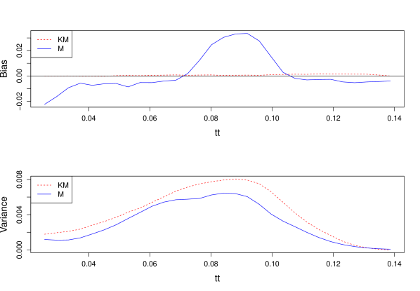
Figure 1: Boostrap estimation of the biases and variances of the prediction error for the two estimators of the cdf ($B=200$, $R=1000$, $N=400$, $\tau=25\%$). $tt$ denotes the time values of the grid ${\cal G}$

Figure 1 shows boostrap estimation of the biases and variances of the prediction error for the two cdf estimators $\hat{F}_{\mbox{\scriptsize KM}}$ and $\hat{F}_{\mbox{\scriptsize M}}$. As expected, the bias of the prediction error is smaller for the estimator $\hat{F}_{\mbox{\scriptsize KM}}$ than for the estimator $\hat{F}_{\mbox{\scriptsize M}}$. In compensation, the variance of the prediction error is weaker for the new estimator. The orders of magnitude of bias and variances are quite similar to those obtained by the model-based simulations (see section 5.2).

Figure 2 presents the cdf $F$ with its two estimators $\hat{F}_{\mbox{\scriptsize KM}}$ and $\hat{F}_{\mbox{\scriptsize M}}$ computed from the initial sample, as well as the 95% bootstrap confidence intervals for $F$ based on formula (10). The confidence interval based on $\hat{F}_{\mbox{\scriptsize M}}$ is more narrow than this based on $\hat{F}_{\mbox{\scriptsize KM}}$ for 83.3 % of the t values of the grid.

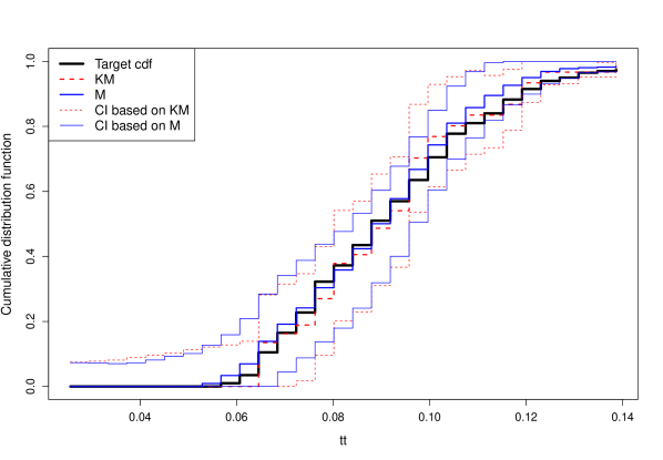
Figure 2: Cdf estimators and the corresponding boostrap estimated 95% confidence intervals for $F$ ($B=200$, $R=1000$, $N=400$, $\tau=25\%$). $tt$ denotes the time values of the grid ${\cal G}$.The target cdf has been computed from the original population ${\cal P}$

5 Model-based simulations

5.1 Description

We present a simulation study to compare the performances of the two cdf estimators $\hat{F}_{\mbox{\scriptsize M}}$ and $\hat{F}_{\mbox{\scriptsize KM}}$, this latter being the naive estimator of the cdf in presence of censoring. We have also derived estimators for the quartiles of the cdf.

At each iteration, a population of size $N$ ($N=200$ and $400$) has been generated according to the accelerated failure time model $\log(t_{j})=-3+0.2*x_{j}+\sigma*u_{j}$ where the covariate $x_{j}$ is uniformly distributed on $(1,4)$. The error term $u_{j}$ follows an extreme value distribution in order to obtain a Weibull distribution for the $t_{j}$. Note that this model is a proportional hazard model with a hazard ratio (HR) equal to $\exp(0.2/\sigma)$ which means that the ratio of the hazard rates of two individuals whose covariate $x$ differs from one unit is constant over time and equal to $\exp(0.2/\sigma)$. Two values of $\sigma$ (0.5 and 0.1) have been chosen leading to hazard ratios of 1.5 and 7.4, which correspond respectively to a weak and a strong relationship between the variable of interest and the auxiliary variable. $t_{j}$ is censored by $c_{j}$ where $c_{j}$ is uniformly distributed on $(0,c)$, $c$ being chosen in order to obtain $0\%$, $10\%$, $25\%$ or $50\%$ of censoring in the whole population. At each iteration, we then draw a simple random sample without replacement of size $n$=$N$/10. $S=1000$ iterations have been performed.

As far as the smoothing is concerned, we choose the triweight kernel $K\left(x\right)=\frac{35}{32}\left(1-x^{2}\right)^{3}1\!\mskip-2.0mu\mbox{I}_{\left(-1,1\right)}\left(x\right)$ rather than the more commonly used Epanechnikov kernel because the triweight kernel is twice differentiable at the boundaries of the interval $\left(-1,1\right)$. So the resulting estimators will have the same degree of regularity. For each iteration $s$, the bandwidths $h_{T}$ and $h_{X}$ have been chosen in a grid of bandwidths so that they minimize the averaged square error (ASE) criterion defined as:

$$\mbox{ASE}(\hat{F}_{\mbox{\scriptsize M,s}})=\displaystyle\frac{1}{K}\sum_{i=1}^{K}\left(\hat{F}_{\mbox{\scriptsize M,s}}(tt_{i})-F_{s}(tt_{i})\right)^{2}.$$

where the evaluation times $tt$ belong to the grid ${\cal G}$ of the $K=30$ regularly spaced values of times between the 5th and the 95th percentiles of the distribution of $t$. Note that this grid is common to all the iterations. The cdf $F_{s}$ is computed for iteration $s$ according to formula (1) using the true $t_{j}$ times.

5.2 Results

The performances of the two estimators have been compared in terms of Monte Carlo bias, variance and mean squared error. For each estimator $\hat{F}$, we compute the estimated bias

$$\widehat{\mbox{B}}(\hat{F}(t))=\displaystyle\frac{1}{S}\sum_{s=1}^{S}\left(\hat{F}_{s}(t)-F_{s}(t)\right),$$

the estimated variance

$$\widehat{\mbox{Var}}(\hat{F}(t))=\displaystyle\frac{1}{S}\sum_{s=1}^{S}\left(\hat{F}_{s}(t)-\frac{1}{S}\sum_{s=1}^{S}\hat{F}_{s}(t)\right)^{2}$$

and the estimated mean squared error (MSE):

$$\widehat{\mbox{MSE}}(\hat{F}(t))=\displaystyle\frac{1}{S}\sum_{s=1}^{S}\left(\hat{F}_{s}(t)-F_{s}(t)\right)^{2}.$$

Note that the usual relationship between the three above quantities does not hold here since the $F_{s}$ function changes as the population is generated at each iteration. In practice, these estimators have been computed on the grid ${\cal G}$ defined above.

The MASE criteria (mean of the estimated MSE over ${\cal G}$) of the estimators have been computed and the ratios $MASE(\hat{F}_{\mbox{\scriptsize KM}})/MASE(\hat{F}_{\mbox{\scriptsize M}})$ are shown in table 1 for two sample sizes, different censoring rates and two strengths of the relationship between the interest variable and the auxiliary variable.

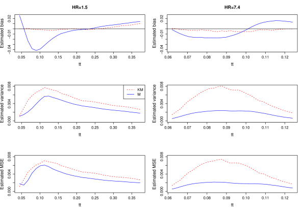
Figure 3: Estimated biases, variances and MSE of the two estimators of the cdf for N=400 individuals, a censoring rate $\tau=25\%$ and the two values of the hazard ratio HR. $tt$ denotes the evalution times of the grid ${\cal G}$

$\hat{F}_{\mbox{\scriptsize M}}$ performs always better than $\hat{F}_{\mbox{\scriptsize KM}}$ with a maximal ratio of the MASE criteria equal to 3.03. As expected, the gain brought by the auxiliary information is much higher when the relationship between the interest variable and the auxiliary variable is great: the ratios of the MASE are more than twice greater when the hazard ratio equals 7.4. For both estimators, the simulations show that the MASE criteria decrease with the sample size and increase with the censoring rate, but the ratios of the MASE criteria remain almost the same for a given hazard ratio.

Figure 3 shows the estimated bias, variance and MSE of the two estimators of the cdf for $N=400$ individuals and a censoring rate $\tau=25\%$ for both hazard ratios. Notice that similar patterns are obtained for other sample sizes and censoring rates. The new estimator has a greater bias than the estimator $\hat{F}_{\mbox{\scriptsize KM}}$ but it shows a smaller variance and MSE for both values of the hazard ratio. As expected, when the relationship between the interest variable and the auxiliary is strong, the bias as well as variance and MSE are appreciably smaller.

Table 1: Estimated ratios $MASE(\hat{F}_{\mbox{\scriptsize KM}})/MASE(\hat{F}_{\mbox{\scriptsize M}})$. $n$ is the sample size, $\tau$ denotes the censoring rate and HR is the hazard ratio of the proportional hazard model describing the relation between $t$ and $x$

	HR=1.5				HR=7.4
n	$\tau$=0%	$\tau$=10%	$\tau$=25%	$\tau$=50%	$\tau$=0%	$\tau$=10%	$\tau$=25%	$\tau$=50%
20	1.27	1.37	1.38	1.59	3.03	2.84	2.85	2.81
40	1.27	1.33	1.34	1.46	2.88	2.96	2.97	2.85

Table 2: Model-based simulation results for the estimation of the quartiles by the two estimators for a weak relationship ($HR=1.5$). Entries indicate relative biases, with square roots of the relavive mean squared errors in parenthesis

	$\tau=0\%$		$\tau=10\%$		$\tau=25\%$		$\tau=50\%$
	Target Q1: 0.080
n	KM	M	KM	M	KM	M	KM	M
20	-0.004	-0.021	0.023	-0.015	0.063	-0.001	0.286	0.049
	(0.330)	(0.128)	(0.397)	(0.115)	(0.519)	(0.211)	(1.054)	(0.453)
40	-0.025	-0.024	-0.021	-0.019	-0.022	-0.017	-0.008	-0.019
	(0.100)	(0.084)	(0.116)	(0.081)	(0.129)	(0.080)	(0.235)	(0.084)
	Target Q2: 0.108
n	KM	M	KM	M	KM	M	KM	M
20	0.074	0.104	0.080	0.107	0.107	0.122	0.246	0.133
	(0.306)	(0.223)	(0.316)	(0.228)	(0.389)	(0.263)	(0.748)	(0.364)
40	0.045	0.100	0.063	0.101	0.074	0.115	0.061	0.099
	(0.187)	(0.195)	(0.199)	(0.197)	(0.209)	(0.212)	(0.233)	(0.205)
	Target Q3: 0.164
n	KM	M	KM	M	KM	M	KM	M
20	0.076	0.089	0.062	0.071	0.083	0.088	0.071	0.015
	(0.295)	(0.228)	(0.281)	(0.217)	(0.320)	(0.247)	(0.441)	(0.237)
40	0.029	0.049	0.047	0.046	0.058	0.055	-0.036	-0.004
	(0.191)	(0.162)	(0.198)	(0.165)	(0.223)	(0.186)	(0.165)	(0.136)

Table 3: Model-based simulation results for the estimation of the quartiles by the two estimators for a strong relationship ($HR=7.4$). Entries indicate relative biases, with square roots of the relavive mean squared errors in parenthesis

	$\tau=0\%$		$\tau=10\%$		$\tau=25\%$		$\tau=50\%$
	Target Q1: 0.075
n	KM	M	KM	M	KM	M	KM	M
20	-0.014	0.011	-0.015	0.015	-0.014	0.016	-0.030	0.012
	(0.092)	(0.037)	(0.095)	(0.038)	(0.107)	(0.044)	(0.139)	(0.057)
40	0.001	0.010	0.003	0.010	0.001	0.012	-0.004	0.013
	(0.046)	(0.026)	(0.053)	(0.027)	(0.059)	(0.030)	(0.077)	(0.034)
	Target Q2: 0.089
n	KM	M	KM	M	KM	M	KM	M
20	-0.003	0.007	-0.004	0.010	-0.005	0.008	-0.010	0.006
	(0.073)	(0.043)	(0.071)	(0.043)	(0.076)	(0.044)	(0.089)	(0.051)
40	-0.006	0.003	-0.004	0.003	0.001	0.006	-0.001	0.004
	(0.056)	(0.039)	(0.056)	(0.040)	(0.060)	(0.041)	(0.069)	(0.045)
	Target Q3: 0.102
n	KM	M	KM	M	KM	M	KM	M
20	-0.016	0.003	-0.015	0.002	-0.020	0.001	-0.035	-0.003
	(0.056)	(0.031)	(0.056)	(0.033)	(0.062)	(0.036)	(0.076)	(0.042)
40	-0.007	0.002	-0.002	0.002	-0.003	0.001	-0.012	0.000
	(0.044)	(0.022)	(0.042)	(0.024)	(0.045)	(0.023)	(0.054)	(0.032)

The estimators of the quartiles have been obtained by numerical inversion of the two cdf estimators. Tables 2 and 3 show the relatives biases and the square roots of the relavive mean squared errors for the different sample sizes and censoring rates, for the two hazard ratios. The results are very similar to those obtained for the cdf estimation: the quartile estimator based on $\hat{F}_{\mbox{\scriptsize KM}}$ has almost always a larger MSE than the quartile estimator based on $\hat{F}_{\mbox{\scriptsize M}}$. As far as the relative bias is concerned, the estimator based on $\hat{F}_{\mbox{\scriptsize M}}$ shows a better performance than the estimator based on $\hat{F}_{\mbox{\scriptsize KM}}$ in half of the cases. Notice that, when the auxiliary variable is strongly linked to the interest variable, the third quartile estimator based on $\hat{F}_{\mbox{\scriptsize M}}$ always behaves better than the estimator based on $\hat{F}_{\mbox{\scriptsize KM}}$ in terms of bias and MSE criterion. Acccording to figure 3, this can be explained by the fact that the curves of the biases of $\hat{F}_{\mbox{\scriptsize M}}$ has very small biases for the $t$ values close to the third quartile.

6 Example

We analyse the data from the Survey of Income and Program Participation (SIPP) with the new method (see Hu and Ridder (2012) for more details about the SIPP). We use the 1992 and 1993 SIPP panels. Each individual is followed up during 36 months. We consider the subsample of monoparental families who benefit from the Aid to Families with Dependent Children program (AFDC). The $t$ variable of interest is the length of time spent on welfare. For simplicity, only the first welfare spell will be considered. The spell is right-censored if it does not end before the family leaves the panel. 520 spells have been recorded, among which 269 are right-censored, leading to a censoring rate $\tau=$51.7%. It has been found in the literature that the benefit level is negatively and significantly related to the probability of leaving welfare: in the SIPP sample, a Cox model explaining the welfare duration by the benefit level gives a hazard ratio of 0.999 (with a p-value of 0.0013). Therefore we use the benefit level as auxiliary variable.

As we need to know the value of the auxiliary variable $x$ for the whole population, we have to consider the above sample of 520 spells as the fixed population ${\cal P}$, in which we draw a sample $s$ of size $n=40$ without replacement. We compute the two cdf estimators $\hat{F}_{\mbox{\scriptsize KM}}$ and $\hat{F}_{\mbox{\scriptsize M}}$ based on the sample $s$ and the auxiliary variable $x$. The bandwidths $h_{T}$ and $h_{X}$ have been chosen by cross-validation according to formula (9). Bootstrap estimated 95% confidence intervals for the cdf based on the two estimators have been obtained by the procedure of section 4 (see formula (10). As the variable of interest is censored in the considered population ${\cal P}$, we cannot compute the true cdf. So, instead of the true cdf, we can use as a target cdf the Kaplan-Meier estimator $\hat{F}_{N}$ computed with all the individuals of ${\cal P}$. The estimators have been computed over the grid of the $K=30$ evaluation times $tt$ regularly spaced between the first and the 99th percentiles of the $t$ values of the sample $s$.

Figure 4 presents the two cdf estimators $\hat{F}_{\mbox{\scriptsize KM}}$ and $\hat{F}_{\mbox{\scriptsize M}}$ as well as the corresponding 95% bootstrap confidence intervals for $F$. Note that the censoring rate of the drawn sample is 42.5%. We also plot as a reference the Kaplan-Meier estimator $\hat{F}_{N}$ computed on ${\cal P}$. The confidence interval based on $\hat{F}_{\mbox{\scriptsize M}}$ is more narrow than this based on $\hat{F}_{\mbox{\scriptsize KM}}$ for all the t values of the grid. The median welfare duration is estimated to 6.68 months by inverting $\hat{F}_{\mbox{\scriptsize KM}}$ and to 10.88 months by inverting $\hat{F}_{\mbox{\scriptsize M}}$. This latter estimation is very close to the estimation of the median welfare duration based on the Kaplan-Meier estimator $\hat{F}_{N}$, which equals 10.79 months.

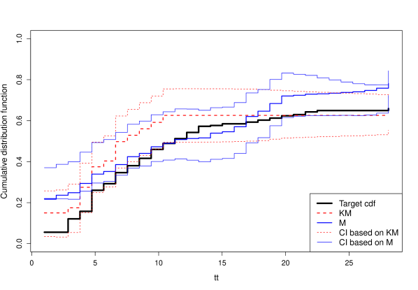
Figure 4: Cdf estimators and the corresponding boostrap estimated 95% confidence intervals for $F$ ($B=200$, $R=1000$) based on a sample of size $n=40$. $tt$ denotes the time values of the grid. The target cdf denotes the Kaplan-Meier estimator $\hat{F}_{N}$ computed on all the individuals of the SIPP sample

7 Design-based simulations

Design-based simulations have been performed: they are based on the SIPP data presented in the previous section. To compare the two estimators, we consider the SIPP sample of size 520 as a fixed population in which we randomly select $S=500$ samples of size 40 without replacement. As in section 6, the true cdf $F$ can not be computed because of censoring. Therefore we use as a target cdf the Kaplan-Meier estimator $\hat{F}_{N}$ computed with all the individuals of the SIPP sample. For each iteration $s$, the bandwidths $h_{T}$ and $h_{X}$ have been chosen in a suitable grid of bandwidths so that they minimize the averaged square error (ASE) criterion defined as:

$$\mbox{ASE}(\hat{F}_{\mbox{\scriptsize M,s}})=\displaystyle\frac{1}{K}\sum_{i=1}^{K}\left(\hat{F}_{\mbox{\scriptsize M,s}}(tt_{i})-\hat{F}_{N}(tt_{i})\right)^{2},$$

where the evaluation times $tt$ belong to the grid ${\cal G^{\prime}}$ of the $K=30$ regularly spaced values between the 5th and the 95th percentiles of the t values of the whole SIPP sample.

The ratio of the MASE criteria (mean of the ASE over the $S$ samples) of the estimator $\hat{F}_{\mbox{\scriptsize KM}}$ over the estimator $\hat{F}_{\mbox{\scriptsize M}}$ is equal to 1.72, which shows clearly the gain brought by the new cdf estimator. Table 4 presents the relative bias and relative root mean squared errors of quartiles estimates of the distribution of the welfare spells. The estimator $\hat{F}_{\mbox{\scriptsize M}}$ has the smallest relative bias except for the median and has always the best performance in terms of relative mean squared error. Figure 5 exhibits the estimated bias and mean squared errors (MSE) of the two cdf estimators. As in the model-based simulations, the bias of $\hat{F}_{\mbox{\scriptsize KM}}$ is very close to zero. On the other hand, $\hat{F}_{\mbox{\scriptsize M}}$ shows a more important bias but a substantially smaller mean squared error than $\hat{F}_{\mbox{\scriptsize KM}}$.

Table 4: Relative biases and relative root mean squared errors (in percentage) of estimates of quartiles of welfare durations ($n=40$)

	Relative bias		Relative root MSE
Target quartile	KM	M	KM	M
$q_{0.25}$= 5.26	26.80	3.18	99.19	36.09
$q_{0.50}$= 10.70	21.54	27.82	51.33	40.15
$q_{0.75}$= 22.60	-14.15	2.79	19.24	12.22

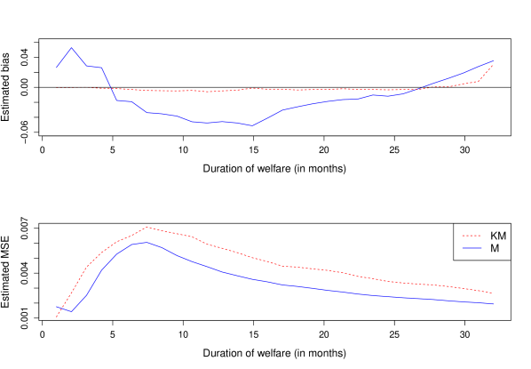
Figure 5: Estimated bias and MSE of the cdf estimators for the welfare duration data

8 Concluding remarks

The simulations show the gain in precision by predicting the interest variable for the non sampled individuals. Therefore it is worth using the estimator $\hat{F}_{\mbox{\scriptsize M}}$ instead of the Kaplan-Meier estimator $\hat{F}_{\mbox{\scriptsize KM}}$ in a finite population when auxiliary information is available.

According to formula (7), it is obvious that $\hat{F}_{\mbox{\scriptsize M}}$ is a step function with jumps among others things at the uncensored time values. As the interest variable is continuous, we expect the cdf to be continuous. So if desired, the cdf estimator $\hat{F}_{\mbox{\scriptsize M}}$ could be smoothed using for instance an integrated kernel as in formula (6), which would require another choice of bandwidth.

The model-based approach is appropriate and will presumably lead to consistent estimators when the sampling is not informative. When a more complex sampling method is used or when the sampling is informative, a model-assisted approach which takes into account the sampling weights would be more adapted. For instance, we can consider the model-assisted parametric cdf estimator of Rao et al (1990) or its non-parametric version proposed by Dorfman and Hall (1993) in the case of simple random sampling. These estimators could be easily generalized to the censored case.

Note that, in panel surveys, nonresponse could be the source of right censoring: in the design-based simulations of section 6, an individual lost to follow-up who was still in welfare state at his last interview is considered as censored. A methodology taking into account the nonresponse could have been more adapted to this case.

The proposed estimators are based on the generalized Kaplan-Meier estimator of the conditional cdf. Other estimators could have been used. In particular, Van Keilegom et al (2001) defined an estimator of the conditional cdf which behaves better than the original Beran estimator in the right tail of the distribution even under heavy censoring. Alternatively, as proposed by Gannoun et al (2005) in the censored case, the conditional median could have been directly estimated by local linear polynomials.

References

- Beran (1981) Beran R (1981) Nonparametric regression with randomly censored survival data. Tech. rep., University of California, Berkeley
- Booth et al (1994) Booth JG, Butler RW, Hall P (1994) Bootstrap methods for finite populations. Journal of the American Statistical Association 89(428):pp. 1282–1289, URL http://www.jstor.org/stable/2290991
- Breslow and Crowley (1974) Breslow NE, Crowley J (1974) A large sample study of the life table and product limit estimates under random censorship. Annals of Statistics 2:437–453, DOI 10.1214/aos/1176342705
- Chambers and Dunstan (1986) Chambers RL, Dunstan R (1986) Estimating distribution functions from survey data. Biometrika 73(3):597–604, DOI 10.1093/biomet/73.3.597
- Dabrowska (1989) Dabrowska DM (1989) Uniform consistency of the kernel conditional kaplan-meier estimate. Annals of Statistics 17:1157–1167
- Dorfman and Hall (1993) Dorfman AH, Hall P (1993) Estimators of the finite population distribution function using nonparametric regression. Annals of Statistics 21:1452–1475
- Efron (1967) Efron B (1967) The two sample problem with censored data. Proc 5th Berkeley Symp 4:831–853
- Földes et al (1980) Földes A, Rejto L, Winter BB (1980) Strong consistency properties of nonparametric estimators for randomly censored: I: the product-limit estimator. Periodica Mathematica Hungarica 11(3):233–250
- Gannoun et al (2005) Gannoun A, Saracco J, Yuan A, Bonney GE (2005) Non-parametric quantile regression with censored data. Scandinavian Journal of Statistics 32(4):527–550
- Hu and Ridder (2012) Hu Y, Ridder G (2012) Estimation of nonlinear models with mismeasured regressors using marginal information. Journal of Applied Econometrics 27(3):347–385, DOI 10.1002/jae.1202, URL http://dx.doi.org/10.1002/jae.1202
- Johnson et al (2008) Johnson AA, Breidt FJ, Opsomer J (2008) Estimating distribution functions from survey data using nonparametric regression. Journal of Statistical Theory and Practice 2:419–431
- Kaplan and Meier (1958) Kaplan E, Meier P (1958) Nonparametric estimation for incomplete observation. Journal of the American Statistical Association 53:457–481
- Kuk (1988) Kuk AYC (1988) Estimation of distribution functions and medians under sampling with unequal probabilities. Biometrika 75(1):pp. 97–103
- Leconte et al (2002) Leconte E, Poiraud-Casanova S, Thomas-Agnan C (2002) Smooth conditional distribution function and quantiles under random censorship. Lifetime Data Analysis 8:229–246
- Li et al (1999) Li KC, Wang JL, Chen CH (1999) Dimension reduction for censored regression data. Annals of Statistics 27:1–23, DOI 10.1214/aos/1018031098
- Lombardia et al (2004) Lombardia MJ, Gonzalez-Manteiga, W, Prada-Sanchez W (2004) Bootstrapping the Dorfman-Hall-Chambers-Dunstan estimate of a finite population distribution function. Journal of Nonparametric Statistics 16(1-2):63–90
- Mukhopadhyay (2001) Mukhopadhyay P (2001) Topics in survey sampling. Lecture notes in statistics, Springer