Tests of hadronic vacuum polarization fits for the muon anomalous magnetic moment

Abstract:

We construct a physically motivated model for the isospin-one non-strange vacuum polarization function $\Pi(Q^{2})$ based on a spectral function given by vector-channel OPAL data from hadronic $\tau$ decays for energies below the $\tau$ mass and a successful parametrization, employing perturbation theory and a model for quark-hadron duality violations, for higher energies. Using a covariance matrix and $Q^{2}$ values from a recent lattice simulation, we then generate fake data for $\Pi(Q^{2})$ and use it to test fitting methods currently employed on the lattice for extracting the hadronic vacuum polarization contribution to the muon anomalous magnetic moment. This comparison reveals a systematic error much larger than the few-percent total error sometimes claimed for such extractions in the literature. In particular, we find that errors deduced from fits using a Vector Meson Dominance ansatz are misleading, typically turning out to be much smaller than the actual discrepancy between the fit and exact model results. The use of a sequence of Padé approximants, recently advocated in the literature, appears to provide a safer fitting strategy.

1 Introduction

Recent measurements of the muon anomalous magnetic moment, $a_{\mu}=(g-2)/2$, have reached an unprecedented level of precision [1]. In the Standard Model (SM), light-quark loop contributions strongly weighted at low-energy make the hadronic contribution to $a_{\mu}$ nonperturbative in the strong coupling $\alpha_{s}$. A numerically important example is the hadronic vacuum polarization (HVP) contribution depicted in Fig. 1. This contribution can be evaluated as an appropriately weighted integral over the electromagnetic spectral function, $\rho_{EM}(s)$, and, luckily, since Nature has solved QCD, $\rho_{EM}$ can be determined experimentally from measured $\sigma(e^{+}e^{-}\rightarrow hadrons)$ data [2]. Adding all other contributions, one finds a SM prediction for $a_{\mu}$ more than 3 sigma away from experiment [1], opening the door to beyond-the-SM speculations. Given the stakes, a reevaluation of this result using completely different techniques is of considerable interest, and the lattice stands out as the only obvious systematic nonperturbative theoretical approach available.

On the lattice, the HVP contribution is given by the integral

$$a_{\mu}^{\rm HVP}=4\alpha^{2}\int_{0}^{\infty}dQ^{2}\,f(Q^{2})\ \big{[}\Pi(0)-\Pi(Q^{2})\big{]}\$$ (1)

with $Q^{2}$ the Euclidean squared momentum and $f(Q^{2})$ a known kernel [3]. A key feature of Eq. (1) is the very strong peaking of the integrand near $Q^{2}\sim m^{2}_{\mu}/4\sim 0.003\ \mathrm{GeV}^{2}$, a scale well below the smallest $Q^{2}$ reachable on typical current lattices (e.g., for the data set considered in Ref. [4], with $1/a=3.3554\ \mathrm{GeV}$ and $T=144$, $Q^{2}_{min}\sim(2\pi/aT)^{2}\sim 0.02143\ \mathrm{GeV}^{2}$). This feature precludes evaluating Eq. (1) as a Riemann sum, making the preliminary step of fitting $\Pi(Q^{2})$ to a known function, which can then be used to evaluate the integral, unavoidable. If the chosen fit function is not capable of reproducing accurately enough the true $\Pi(Q^{2})$ in the region of the peak of the integrand, this step introduces a systematic error which contaminates the final result for $a_{\mu}$. It is of course very difficult to assess this systematic error without knowing the true $\Pi(Q^{2})$. A good model can help provide a benchmark for assessing this systematic error. We briefly summarize the analysis based on such a model, which has recently appeared in Ref. [5], in what follows.

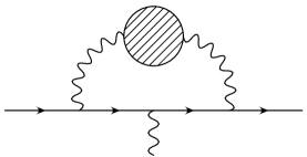
Figure 1: Vacuum polarization contribution to $a_{\mu}$. The shaded blob contains only quarks and gluons, wavy lines are photons and the solid line is the muon.

2 The Model

We define the model vacuum polarization function by the once-subtracted dispersion relation

$$\Pi(Q^{2})=-Q^{2}\int_{4m_{\pi}^{2}}^{\infty}dt\;\frac{\rho(t)}{t(t+Q^{2})}\ ,$$ (2)

with the spectral function $\rho(t)$ determined as follows. In the region $4m_{\pi}^{2}\leq t\leq s_{min}\leq m_{\tau}^{2}$, we use the non-strange $I=1$ vector-channel OPAL spectral data, updated for current branching fractions, while, for $s_{min}\leq t<\infty$, we use the parametrization

$$\rho_{t\geq s_{min}}(t)=\rho_{\rm pert}(t)+\rho_{\rm DV}(t)\quad,\quad\rho_{\rm DV}(t)=e^{-\delta-\gamma\,t}\sin(\alpha+\beta t)\ ,$$ (3)

where $\rho_{\rm pert}$ is the spectral function calculated to five loops ($O\left(\alpha_{s}^{4}\right)$) in perturbation theory [6], and $\rho_{\rm DV}$ models effects due to quark-hadron duality violations. These duality violations are due to the presence of resonances in the spectrum and cannot be captured by the Operator Product Expansion. The values used for the parameters $s_{min},\alpha,\beta,\delta,\gamma$ can be found in Ref. [5]. This parametrization of $\rho(t)$ was developed in Ref. [8], building on earlier ideas discussed in Ref. [9], and has been extensively studied in Refs. [7] in the context of a determination of $\alpha_{s}$ from hadronic $\tau$ decay data. Figure 2 shows how well this parametrization is able to describe the experimental data.

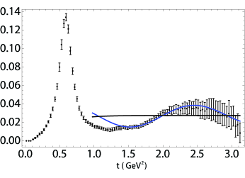
Figure 2: The $I=1$ non-strange vector spectral function, from Ref. [7]. Experimental data is from OPAL [10]. The black solid line is the result of perturbation theory, $\rho_{\rm pert}(t)$, and the blue solid line the result after adding our parametrization of duality violations, $\rho_{\rm DV}(t)$, described in the text.

To focus our tests on the potentially problematic, very low $Q^{2}$ region of the $a_{\mu}^{\rm HVP}$ integral in (1), we use as benchmark the $Q^{2}\leq 1\ \mathrm{GeV}^{2}$ contributions in the model

$$\widetilde{a}_{\mu}^{\mathrm{HVP},Q^{2}\leq 1}=4\alpha^{2}\int_{0}^{1\mathrm{GeV}^{2}}dQ^{2}\,f(Q^{2})\ \big{\{}\Pi(0)-\Pi(Q^{2})\big{\}}=1.204\times 10^{-7}\ .$$ (4)

Results using various fit strategies will be compared to this below. The tilde in $\widetilde{a}_{\mu}^{\rm HVP}$ distinguishes the $I=1$ model result from the true value in nature, $a_{\mu}^{\rm HVP}$. As can be seen from Eq. (2), the model $\Pi(Q^{2})$ is already subtracted at $Q^{2}=0$ and hence satisfies $\Pi(0)=0$.

3 Generation of fake lattice data and fit functions

We focus on the discrete set $\{Q_{i}^{2}\}$ of $Q^{2}$ values available on a $L^{3}\times T=64^{3}\times 144$ lattice with periodic boundary conditions and inverse lattice spacing $1/a=3.3554$ GeV [4]. The smallest squared momentum is then $(2\pi/aT)^{2}=0.02143\ \mathrm{GeV}^{2}$, significantly larger than the scale $\sim m^{2}_{\mu}/4=0.003\ \mathrm{GeV}^{2}$ at which the strong peak of the integrand in Eq. (1) occurs (cf. Fig. 3 below). For these $Q_{i}^{2}$ we have constructed a multivariate Gaussian distribution with central values $\Pi(Q_{i}^{2})$ and a covariance matrix set equal to that of the real lattice data of Ref. [4]. A fake data set is then obtained by drawing one random sample from this distribution. This sample will be the one to be used in all our comparisons below.

As a family of fit functions, we use the sequence of Padé approximants described in Ref. [4],

$$\Pi(Q^{2})=\Pi(0)-Q^{2}\left(a_{0}+\sum_{k=1}^{K}\frac{a_{k}}{b_{k}+Q^{2}}\right)\ .$$ (5)

For $a_{0}=0$ the term in parentheses is a $[K-1,K]$ Padé, whereas if $a_{0}$ is a free parameter we have a $[K,K]$ Padé. This sequence is known to converge to the vacuum polarization (VP) function.

As noted above, the model VP function, $\Pi(Q^{2})$, is already subtracted at $Q^{2}=0$ and satisfies $\Pi(0)=0$. The $\Pi(Q^{2})$ measured on the lattice, in contrast, is unsubtracted, with $\Pi(0)$ determined by the fit. A faithful simulation of the lattice situation may, however, be obtained by leaving the parameter $\Pi(0)$ appearing in the fit function (4) free and determining its value in the fit [5].

Vector Meson Dominance-type (VMD-type) fits have been frequently used in the literature [11]. In its simplest incarnation, VMD corresponds to taking $K=1$ and $a_{0}=0$ in Eq. (4) and fixing $b_{1}=m_{\rho}^{2}$. An extended version, which we will call VMD+, is obtained by making $a_{0}$ a free, in general non-zero, fit parameter. It is important to realize that, despite appearances, VMD-type functions are not elements of the Padé sequence known to converge to the true VP function. From the point of view of the analytic properties of $\Pi(Q^{2})$, whose discontinuity is produced by a cut starting at $Q^{2}=-4m_{\pi}^{2}$ rather than a simple pole, the choice $b_{1}=m_{\rho}^{2}$ seems somewhat arbitrary. Padés converge to the true function because their poles pile up in such a way that they resemble the cut, and it is hard to imagine how this could also happen if certain poles are fixed at some predetermined values, as in VMD. In fact, as we will see in the next section, our model yields convincing evidence that VMD-type fits are unreliable at the level of precision desired in the $a_{\mu}^{HVP}$ problem.

4 Results

	$\widetilde{a}_{\mu}^{\mathrm{HVP},Q^{2}\leq 1}\times 10^{7}$	Error$\times 10^{7}$	$\chi^{2}/\mathrm{dof}$	Pull
VMD	1.3201	0.0052	2189/47	-
VMD+	1.0658	0.0076	67.4/46	18
$[0,1]$	0.8703	0.0095	285/46	-
$[1,1]$	1.116	0.022	61.4/45	4
$[1,2]$	1.182	0.043	55.0/44	0.5
$[2,2]$	1.177	0.058	54.6/43	0.5

Table 1: Results of different types of fits to a realistic set of lattice data. See text.

Results of correlated fits to the fake data set, constructed using the covariance matrix employed to generate that data, are shown in Table 1. The first column gives the fit function form, the second the result obtained for $\widetilde{a}_{\mu}^{\mathrm{HVP},Q^{2}\leq 1}$, using Eq. (4) and the fitted version of that function. The resulting statistical error on $\widetilde{a}_{\mu}^{\mathrm{HVP},Q^{2}\leq 1}$ is shown in column 3 and the $\chi^{2}/\mathrm{dof}$ for the fit in column 4. The last column shows the “Pull”, a measure of the reliability of the fit, defined to be the ratio of the true error to the fit error, i.e.,

$$\mathrm{Pull}=\frac{\mathrm{exact\ value}-\mathrm{fit\ value}}{\mathrm{error}}\ .$$ (6)

A reliable fit should have an error comparable to the difference between the exact and fit values, i.e. a Pull $\lesssim 1$. Recall that the exact result, given in Eq. (4), is $\widetilde{a}_{\mu}^{\mathrm{HVP},Q^{2}\leq 1}=1.204\times 10^{-7}$.

From Table 1 we observe that the small error obtained from the VMD fit is very misleading, though the large $\chi^{2}/\mathrm{dof}$ is at least a warning that the fit is bad and should not be trusted. We have thus refrained from quoting the corresponding Pull. More worrisome is the result for VMD+. The fit is apparently good, with a $\chi^{2}/\mathrm{dof}$ acceptably close to $1$, but, despite the very small error obtained from the fit, the value for $\widetilde{a}_{\mu}^{\mathrm{HVP},Q^{2}\leq 1}$ is totally wrong, as emphasized by a very large Pull. The result based on this fit has a systematic error which the $\chi^{2}/\mathrm{dof}$ completely fails to expose!

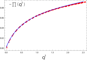
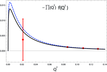
Figure 3: Left panel: VMD+ fit to the fake data corresponding to the model $\Pi(Q^{2})$. Right Panel: (Black solid curve) Result of the fit in the left panel for the integrand of $\widetilde{a}_{\mu}^{\mathrm{HVP}}$, Eq. (1.1). (Blue dashed curve) The corresponding exact model result.

The source of the misleading nature of the result for $\widetilde{a}_{\mu}^{\mathrm{HVP},Q^{2}\leq 1}$ obtained from the VMD+ fit can be understood from Fig. 3. The left panel shows the result of the VMD+ fit for the VP function $\Pi(Q^{2})$. The fit looks very good, as corroborated by the decent $\chi^{2}/\mathrm{dof}=67.4/46$ shown in Table 1. This, however, obscures the fact (shown in the right panel) that, in the region where the integrand gets most of its contribution (and where no data exists!) the fit (depicted by the black solid curve) significantly misrepresents the exact result (depicted by the blue dashed curve), leading to the wrong estimate for the integral shown in Table 1, and the consequent large value, $18$, for the Pull. The moral of this exercise is twofold. First, it is potentially very misleading to judge the reliability of the value of $\widetilde{a}_{\mu}^{\mathrm{HVP},Q^{2}\leq 1}$ obtained from a given fit based solely on the agreement of the fit and data versions of the VP function; a plot of the fit and data versions of the integrand is safer in this regard. Second, since the source of the problem is a failure of the fitted version to adequately represent the curvature of $\Pi(Q^{2})$ at those $Q^{2}$ lying outside the fit window, and hence an insufficiently accurate extrapolation from the lowest $Q^{2}$ data point down to $Q^{2}$ in the vicinity of the peak of the integrand, the more precise data one has in the peak region and/or just above it, the more likely it will be that the error coming out of the fit will be reliable.

Concerning the Padés, one sees that although the first elements in the sequence (i.e. the $[0,1]$ and the $[1,1]$ Padés) do not do a great job, as witnessed by the corresponding $\chi^{2}/\mathrm{dof}$, by the time the $\chi^{2}/\mathrm{dof}$ is close to $1$ the error extracted from the fit is reliable, giving Pulls $<1$. This is the case for the $[1,2]$ and $[2,2]$ Padés. Space constraints preclude displaying the Padé analogues of Fig. 3. The $[1,2]$ Padé version is, however, presented in Ref. [5] and shows a left panel essentially identical to that of Fig. 3. The right panel, however, is completely different, the solid black and dashed blue curves now lying almost on top of one another. The Padés approach thus appears to represent a more reliable fit strategy. Note, however, that the final error for $\widetilde{a}_{\mu}^{\mathrm{HVP},Q^{2}\leq 1}$ obtained using the $[1,2]$ and $[2,2]$ Padés is $\sim 4-5\%$. Since other sources of error (chiral and continuum extrapolation, finite size effects, disconnected diagrams, etc…) have yet to be added, we conclude that few $\%$ total error estimates for current lattice determination of $a_{\mu}^{\mathrm{HVP}}$ must be considered unrealistic.

In view of the $\sim 1\%$ error claimed for the determination of $a_{\mu}^{\mathrm{HVP}}$ based on experimental electroproduction cross-sections [2], we have also performed the following exercise. Keeping the data and $\{Q_{i}^{2}\}$ set the same, we have divided the errors by a factor of $\sim$ 100 (i.e., the covariance matrix by a factor of $10^{4}$) and then generated (randomly) a new fake data set. Though clearly not realistic for near-future lattice determinations, this “Science Fiction” scenario allows us to investigate whether such a drastic “brute-force” error reduction would allow the lattice to achieve a competitive ($\sim 1\%$) determination of $a_{\mu}^{\mathrm{HVP}}$. The answer we find is “barely.” The results of the corresponding fits are shown in Table 2.

	$\widetilde{a}_{\mu}^{\mathrm{HVP},Q^{2}\leq 1}\times 10^{7}$	Error$\times 10^{7}$	$\chi^{2}/\mathrm{dof}$	Pull
VMD	1.31861	0.00005	2$\times 10^{7}$/47	-
VMD+	1.07117	0.00008	7$\times 10^{4}$/46	-
$[0,1]$	0.87782	0.00009	2$\times 10^{7}$ /46	-
$[1,1]$	1.0991	0.0002	5 $\times 10^{4}$/45	-
$[1,2]$	1.1623	0.0004	1340/44	-
$[2,2]$	1.1862	0.0015	76.4/43	12
$[2,3]$	1.1965	0.0028	42.0/42	2

Table 2: Results of the same type of fits to a “Science Fiction” lattice data set, with a 100 times smaller errors.

One sees in Table 2 that VMD and VMD+ are incapable of producing a decent fit (i.e., the $\chi^{2}$ is simply huge). While low-order Padés have the same problem, the general convergence property comes to the rescue once sufficiently high orders are reached. This happens for the $[2,3]$ Padé. However, even then the Pull is $2$, i.e., the error from the fit underestimates the true discrepancy with the exact value ($0.6\%$) by a factor of 2. The obvious conclusion seems to be that major improvements in the determination of $a_{\mu}^{\mathrm{HVP}}$ will require a denser set of data points close to the integrand peak shown in Fig. 3. This points to the use of larger lattice volumes and/or twisted boundary conditions. The recent proposals of Refs. [12] may also help.

5 Conclusions

Current lattice determinations of $a_{\mu}^{\mathrm{HVP}}$ require the use of a fit function to extrapolate data to the much lower $Q^{2}$ dominating the integral representation (1) of $a_{\mu}^{\mathrm{HVP}}$. Comparisons in a model context, where the exact value is known, show that VMD-type fits are not reliable, failing to achieve an accuracy of even a few $\%$. Padé approximants of sufficiently high order represent a more promising approach.

We have shown that, as a consequence of the non-trivial curvature of $\Pi(Q^{2})$ in the low-$Q^{2}$ region, the $\chi^{2}/\mathrm{dof}$ of a fit cannot, in general, be used to assess the reliability of the associated result for $a_{\mu}^{\mathrm{HVP}}$ unless very good data is available in and/or near the region of the peak of the integrand in Eq. (1). Plots of the fit to $\Pi(Q^{2})$ may thus be very misleading, and alternate forms showing the data and fit versions of the integrand in Eq. (1) serve better to reveal the quality of those aspects of the fit to the data most relevant to a reliable determination of $a_{\mu}^{\mathrm{HVP}}$.

In lattice calculations, where the underlying exact $\Pi(Q^{2})$ is not known a priori, our results show the importance of a quantitative assessment of the systematic error associated with the use of particular fit functions and methods. We encourage all future lattice calculations to include such assessments, which can be obtained by using the $Q^{2}$ values and covariance matrix of the lattice data entering the fits to generate a set of fake data with the model for $\Pi(Q^{2})$ presented here. While achieving a $\lesssim 1\%$ lattice determination of $a_{\mu}^{\mathrm{HVP}}$ won’t be a rose garden, it is very important to try.

References

- [1] G. W. Bennett et al. [Muon G-2 Collaboration], Phys. Rev. D 73, 072003 (2006) [hep-ex/0602035].
- [2] T. Teubner et al., Nucl. Phys. Proc. Suppl. 225-227, 282 (2012); M. Davier et al., Eur. Phys. J. C 71, 1515 (2011) [Erratum-ibid. C 72, 1874 (2012)] [arXiv:1010.4180 [hep-ph]].
- [3] T. Blum, Phys. Rev. Lett. 91, 052001 (2003) [hep-lat/0212018]; B. E. Lautrup et al., Phys. Rept. 3, 193 (1972).
- [4] C. Aubin, T. Blum, M. Golterman and S. Peris, Phys. Rev. D 86, 054509 (2012) [arXiv:1205.3695 [hep-lat]]; C. Aubin et al., PoS LATTICE 2012, 176 (2012) [arXiv:1210.7611 [hep-lat]].
- [5] M. Golterman, K. Maltman and S. Peris, [arXiv:1309.2153 [hep-lat]].
- [6] P. A. Baikov et al., Phys. Rev. Lett. 101, 012002 (2008) [arXiv:0801.1821 [hep-ph]].
- [7] D. Boito et al., Phys. Rev. D 84, 113006 (2011) [arXiv:1110.1127 [hep-ph]]; D. Boito et al., Phys. Rev. D 85, 093015 (2012) [arXiv:1203.3146 [hep-ph]].
- [8] O. Catà, M. Golterman and S. Peris, Phys. Rev. D 77, 093006 (2008) [arXiv:0803.0246 [hep-ph]].
- [9] M. A. Shifman, In *Shifman, M. (ed.): At the frontier of particle physics, vol. 3* 1447-1494 [hep-ph/0009131] and references therein; O. Catà, M. Golterman and S. Peris, JHEP 0508, 076 (2005) [hep-ph/0506004]; M. Golterman et al., JHEP 0201, 024 (2002) [hep-ph/0112042].
- [10] K. Ackerstaff et al. [OPAL Collaboration], Eur. Phys. J. C 7, 571 (1999) [hep-ex/9808019].
- [11] M. Della Morte et al., JHEP 1203, 055 (2012) [arXiv:1112.2894 [hep-lat]]; C. Aubin and T. Blum, Phys. Rev. D 75, 114502 (2007) [hep-lat/0608011]; X. Feng et al., Phys. Rev. Lett. 107, 081802 (2011) [arXiv:1103.4818 [hep-lat]]; P. Boyle et al., Phys. Rev. D 85, 074504 (2012) [arXiv:1107.1497 [hep-lat]]; F. Burger et al., arXiv:1308.4327 [hep-lat].
- [12] G. M. de Divitiis et al., Phys. Lett. B 718, 589 (2012) [arXiv:1208.5914 [hep-lat]]; X. Feng et al., Phys. Rev. D 88, 034505 (2013) [arXiv:1305.5878 [hep-lat]].