Cavity method for force transmission in jammed disordered packings of hard particles

Abstract

The force distribution of jammed disordered packings has always been considered a central object in the physics of granular materials. However, many of its features are poorly understood. In particular, analytic relations to other key macroscopic properties of jammed matter, such as the contact network and its coordination number, are still lacking. Here we develop a mean-field theory for this problem, based on the consideration of the contact network as a random graph where the force transmission becomes a constraint optimization problem. We can thus use the cavity method developed in the last decades within the statistical physics of spin glasses and hard computer science problems. This method allows us to compute the force distribution $\text{P}(f)$ for random packings of hard particles of any shape, with or without friction. We find a new signature of jamming in the small force behavior $\text{P}(f)\sim f^{\theta}$, whose exponent has attracted recent active interest: we find a finite value for $\text{P}(f=0)$, along with $\theta=0$. Furthermore, we relate the force distribution to a lower bound of the average coordination number $\,{\bar{z}}_{\rm c}^{\rm min}(\mu)$ of jammed packings of frictional spheres with coefficient $\mu$. This bridges the gap between the two known isostatic limits $\,{\bar{z}}_{\rm c}(\mu=0)=2D$ (in dimension $D$) and $\,{\bar{z}}_{\rm c}(\mu\to\infty)=D+1$ by extending the naive Maxwell’s counting argument to frictional spheres. The theoretical framework describes different types of systems, such as non-spherical objects in arbitrary dimensions, providing a common mean-field scenario to investigate force transmission, contact networks and coordination numbers of jammed disordered packings.

Mechanically stable packings of granular media are important to a wide variety of technical processes Behringer and Jenkins (1997). One approach to characterize jammed granular packings is via the interparticle contact force network. In turn, this network determines the probability density of inter-particle contact forces $\text{P}(f)$ and the average coordination number ${\bar{z}}$. While the force network has been studied for years, there is yet no unified theoretical framework to explain the common observations in granular packings, ranging from frictional to frictionless systems, from spherical to non-spherical particles and in any dimensions.

Experimental force measurements Zhou et al. (2006); Liu et al. (1995); Mueth et al. (1998); Løvoll et al. (1999); Erikson et al. (2002); Brujić et al. (2003, 2003) and simulations Radjai et al. (1996); O’Hern et al. (2001); Tkachenko and Witten (2000); Makse et al. (2000) have shown that the interparticle forces are inhomogeneously distributed with common features: $\text{P}(f)$ near the jamming transition has a peak at small forces and an approximate exponential tail in the limit of large $f$. It is argued that the development of a peak is a signature of the jamming transition O’Hern et al. (2001). The scaling of $\text{P}(f)$ in the limit of small forces is directly related to the mechanical stability of the packing Wyart (2012); Lerner et al. (2013): the contacts bearing small loads are the ones for which a local buckling is the most easily achieved Lerner et al. (2013), and they must thus exist in small enough density for the packing to be stable. Some parts of the qualitative behavior of $\text{P}(f)$ are correctly captured by simplified mean-field models, such as the q-model Liu et al. (1995); Coppersmith et al. (1996) and Edwards’ model Brujić et al. (2003, 2003). Both of them describe the exponential decay at large force and a power law behavior $\text{P}(f)\sim f^{\theta}$ for small forces Brujić et al. (2003, 2003); Socolar (1998). However, the exponent $\theta$ obtained by the q-model (an integer $\theta\geq 1$ Liu et al. (1995); Socolar (1998)) is larger than the one obtained by recent numerical simulations accessing the low force limit with increasing accuracy $0.2\lesssim\theta\lesssim 0.5$ Charbonneau et al. (2012); Lerner et al. (2013), while the exponent obtained by Edwards’ model $\theta=1/({\bar{z}}-2)$ depends strongly on the dimension (through ${\bar{z}}$), when simulations show it does not Charbonneau et al. (2012). A recent replica calculation finds an exponent $\theta\approx 0.42$ in infinite dimensions of space Kurchan et al. (2013); Charbonneau et al. (2013, 2014). Other theoretical approaches based on entropy maximization similar to Edwards’ statistical mechanics Edwards and Oakeshott (1989) also recover the large force exponential decay Kruyt and Rothenburg (2002); Bagi (2003); Goddard (2004); Henkes and Chakraborty (2009). Some of those works which simulated the force network ensemble Snoeijer et al. (2004) on strongly hyperstatic ${\bar{z}}=6>\,{\bar{z}}_{\rm c}$ triangular lattice Tighe et al. (2008) and on 2-D (3-D) disordered hyperstatic frictionless bead packings generated using molecular dynamics van Eerd et al. (2007) however predict a force distribution that decays faster than exponential, and so does a mean-field theory based on replica theory of spin glasses Charbonneau et al. (2012); Parisi and Zamponi (2010); Berthier et al. (2011). Recent measurements in the bulk of packings Zhou et al. (2006); Brujić et al. (2003, 2003); Majmudar and Behringer (2005) find downward curvature on semi-log plot of $\text{P}(f)$.

The average coordination number per particle ${\bar{z}}$ is another key signature of jamming. Close to jamming, many observables (pressure, volume fraction, shear modulus or viscosity Lerner et al. (2012) to name a few) scale with the distance ${\bar{z}}-\,{\bar{z}}_{\rm c}$ to the average coordination number $\,{\bar{z}}_{\rm c}$ at the transition. Understanding the value of $\,{\bar{z}}_{\rm c}$ is thus of primary importance. The case of frictionless spheres, for which, $\,{\bar{z}}_{\rm c}=2D$ where $D$ is the dimension, has been rationalized based on counting arguments leading to the isostatic conjecture Alexander (1998); Tkachenko and Witten (1999); Moukarzel (1998): a lower bound $\,{\bar{z}}_{\rm c}\geq 2D$ is provided by Maxwell’s stability argument Maxwell (1864), and an upper bound $\,{\bar{z}}_{\rm c}\leq 2D$ is given by the geometric constraint of having the particles exactly at contact, without overlap. The problem, however, turns out to be more complicated when friction is considered, and no method is known so far to predict $\,{\bar{z}}_{\rm c}$ in such a case. The (naive) generalization of the counting arguments gives the bounds $D+1\leq\,{\bar{z}}_{\rm c}\leq 2D$ in frictional packings, independently of the value of the interparticle friction coefficient $\mu$. Indeed, there is a range of $\,{\bar{z}}_{\rm c}$ obtained numerically and experimentally Snoeijer et al. (2004); Moukarzel (1998); Silbert et al. (2002, 2002); Zhang and Makse (2005); Shundyak et al. (2007); Song et al. (2008); Wang et al. (2010); Silbert (2010); Papanikolaou et al. (2013); Brujić et al. (2007). However, for small $\mu$, this range never extends to the predicted lower bound, as packings with low friction coefficient lie close to $\,{\bar{z}}_{\rm c}=2D$.

Here we present a theoretical framework at a mean-field level to consider force transmission as a constraint optimization problem on random graphs, and study this problem with standard tools, namely the cavity method M. Mezard and Virasoro (1986). We first obtain the force distribution for spheres, in frictionless and frictional cases, both in two and three dimensions. Besides showing the experimentally known approximate exponential fall-off at large forces, these distributions bring a new insight in the much less known small force regime. In particular, we find for frictionless spheres in both 2 and 3 dimensions a finite value for $\mathrm{P}(f)$ in $f=0$, leading to a mean-field exponent $\theta=0$ for small forces.

Our framework is also the first one to show theoretically how the frictional coefficient $\mu$ affects the average number of contacting neighbors $\,{\bar{z}}_{\rm c}$ at the jamming transition, and we find a lower bound $\,{\bar{z}}_{\rm c}^{\rm min}(\mu)$ for this number (which is also a lower bound on ${\bar{z}}$, since ${\bar{z}}\geq\,{\bar{z}}_{\rm c}$ in a packing). We achieve this by generalizing in a careful way the naive Maxwell counting arguments, considering the satisfiability of force and torque balances equations. Linking $\,{\bar{z}}_{\rm c}$ to the behavior of force and torque balances is not a new idea, as it was already suggested by Silbert et al. Silbert et al. (2002). Furthermore the generalized isostaticity picture Shundyak et al. (2007) gives a bound on the number of fully mobilized forces (ie the number of tangential forces which are taking the maximally value allowed by the Coulomb law) based on the value of $\,{\bar{z}}_{\rm c}$. However, none of these works derive a bound for $\,{\bar{z}}_{\rm c}$ itself, at a given $\mu$. The bound $\,{\bar{z}}_{\rm c}^{\rm min}(\mu)$ that we obtain interpolates smoothly between the two isostatic limits at $\mu=0$ and $\mu\to\infty$.

I Force and torque balances as a satisfiability problem

A packing can be described as an ensemble of particles with given position and orientation, having interparticle contacts such that (i) there is no overlap between particles, (ii) force and torque balances are satisfied on every particle, and (iii) the packing is rigid, ie there is no displacement of particles, individual or collective, that does not create a violation of conditions (i) or (ii) (except for global translation or rotation of the packing). In this work, we consider the geometric configuration as given (ie condition (i) is fulfilled and taken for granted), hence we do not discuss about the spatial degrees of freedom but rather focus on the force degrees of freedom.

Now, let us argue that, in the case of random packings of spheres under finite pressure, fulfilling condition (ii) (force and torque balances) implies that condition (iii) (stability) is also fulfilled. Force and torque balances under finite pressure ensure (by definition) that the system is stable against isotropic compression. The average force in the packing is then proportional to the pressure. But, as such, nothing is guaranteed concerning the stability of the packing against more general perturbations, as defined by the condition (iii). In the case of sphere packings, however, it is very likely that packings verifying force and torque balances while still being mechanically unstable have some sort of order, at least locally (one can think of the case of a row of frictionless spheres perfectly aligned for example, which can maintain force balance, but is unstable). This is what is observed at the jamming transition, when packings prepared under isotropic pressure are naturally stable O’Hern et al. (2003). Hence, for random packings of spheres, the requirement of force and torque balances is argued to be enough for having stability too, ie conditions (ii) and (iii) are simultaneously fulfilled.

Similarly to the global rigidity condition, force and torque balances are entirely constrained by the contact network of the packing. If we define $\vec{r}^{\,a}_{i}$ as the vector joining the center of particle $a$ and the contact $i$ on it, the contact network is uniquely defined by the complete set $\{\vec{r}^{\,a}_{i}\}$. Calling $\vec{f}^{\,a}_{i}$ the force acting on particle $a$ from contact $i$, force and torque balances read:

$$\begin{array}[]{llr}\displaystyle\sum_{i\in\partial a}\vec{f}^{\,a}_{i}=0,&\vec{r}^{\,a}_{i}\cdot\vec{f}^{\,a}_{i}<0,&\hbox{\multirowsetup$\qquad\forall\,a$}\\ \displaystyle\sum_{i\in\partial a}\vec{r}^{\,a}_{i}\times\vec{f}^{\,a}_{i}=0,&f_{i}^{\,t}\leq\mu f_{i}^{\,n},&\end{array}$$ (1)

where the notation $\partial a$ denotes the set of contacts of particle $a$. We explicitly take into account friction by decomposing the force into normal and tangential parts $\vec{f}^{\,a}_{i}=-f_{i}^{\,n}\hat{n}^{\,a}_{i}+f_{i}^{\,t}\hat{t}^{\,a}_{i}$, where $\hat{n}^{\,a}_{i}$ and $\hat{t}^{\,a}_{i}$ are normal and tangential unit vectors to the contact, respectively. The inequality $\vec{r}^{\,a}_{i}\cdot\vec{f}^{\,a}_{i}<0$ ensures the repulsive nature of the normal force. The last inequality ensures Coulomb’s law with friction coefficient $\mu$.

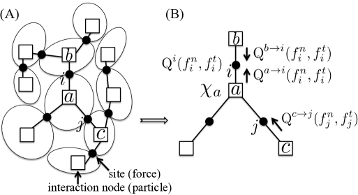
Figure 1: Factor graph and variables. (A) Building the factor graph of contacts from a packing Mezard and Montanari (2009). The contacts becomes sites (filled circles) with associated variables being forces. The particles are reduced to interaction nodes (open squares) dealing with force/torque balance Eq. (1). (B) Part of factor graph used to compute $\text{Q}^{i}$ and $\text{Q}^{a\to i}$ by using Eq. (5) and Eq. (6). On the edges around particle $a$, the arrows indicate that we consider the force probabilities $\text{Q}^{\to}$ as ‘messages’ going through contacts in the contact network. In our algorithm, $\text{Q}^{a\to i}$ is iteratively updated by the uncorrelated force probability $\text{Q}^{c\to j}$ on neighboring edges with the force/torque balance constraint $\chi_{a}(\{f^{\,n},f^{\,t},\hat{n}^{\,a},\hat{t}^{\,a}\}_{\partial a})$ on that particle $a$, verifying the cavity equation Eq. (6). The marginal probability $\text{Q}^{i}(f_{i}^{\,n},f_{i}^{\,t})$ on site $i$ is calculated as a product of $\text{Q}^{a\to i}$ and $\text{Q}^{b\to i}$ as in Eq. (5).

The constraints induced by force and torque balances on the forces $\vec{f}_{i}$ are not always satisfiable. In the case of frictionless spheres, we can recover the known ${\bar{z}}\geq 2D$ directly from force balance alone. The naive Maxwell counting argument Moukarzel (1998) applied to frictionless spheres reduces Eq. (1) to a set of linear equations by taking into account only force balance and neglecting the repulsive nature of the forces. Maxwell argument considers the minimal number of forces needed to satisfy Eq. (1) which gives, per sphere, $D$ equations and ${\bar{z}}/2$ variables (forces), implying ${\bar{z}}\geq 2D$ to have a solution. Below this threshold, there is generically no solution to Eq. (1). To accurately extend this counting argument to more general conditions (frictional, repulsive, and/or non-spherical particles), one must take into account all the constraints in Eq. (1), including the repulsive nature of the forces and the Coulomb condition for frictional packings. Indeed, the naive Maxwell argument, neglecting those constraints, concludes ${\bar{z}}>\,\,{\bar{z}}_{\rm c}^{\rm min}(\mu)=D+1$ for any frictional packing of spheres, ignoring the dependance on the friction coefficient Edwards and Grinev (1999). On the other hand, below we show that including the above mentioned constraints we obtain an accurate lower bound $\,{\bar{z}}_{\rm c}^{\rm min}(\mu)$, explicitely depending on $\mu$.

We tackle the problem of satisfiability of force and torque balances Eq. (1) by looking at the contact network in an amorphous packing as an instance of random graph. As depicted in Fig. 1A, starting from a packing of $N$ particles, we explicitly construct a so-called factor graph Mezard and Montanari (2009), considering the $M={\bar{z}}N/2$ contacts as ‘sites’, and the $N$ particles as ‘interaction nodes’. Each site $i$ bears two vectors $\vec{r}^{\,a}_{i}$ and $\vec{r}^{\,b}_{i}$ and two opposite forces $\vec{f}^{\,a}_{i}=-\vec{f}^{\,b}_{i}$ (one per particle involved in the contact). Note that $\{\hat{n}^{\,a}_{i}\}$ are uniquely determined by the contact network $\{\vec{r}^{\,a}_{i}\}$ and represents the ‘quenched’ disorder in the system, whereas $\{\hat{t}^{\,a}_{i}\}$ are free to rotate in the plane tangent to contact. On each interaction node (particle) $a$, we enforce force balance, torque balance, repulsive interactions and Coulomb friction conditions on its $z_{a}$ neighboring sites by an interaction function,

$$\begin{array}[]{rl}\chi_{a}(\{f^{\,n},f^{\,t},\hat{n}^{\,a},\hat{t}^{\,a}\}_{\partial a})=&\!\!\!\!\delta\Big{(}\displaystyle\sum_{i\in\partial a}\vec{f}^{\,a}_{i}\Big{)}\>\delta\Big{(}\displaystyle\sum_{i\in\partial a}\vec{r}^{\,a}_{i}\times\vec{f}^{\,a}_{i}\Big{)}\\ &\quad\times\displaystyle\prod_{i\in\partial a}\Theta(f_{i}^{\,n})\Theta(\mu f_{i}^{\,n}-f_{i}^{\,t}).\end{array}$$ (2)

We define the partition function $Z$ and entropy $S$ for the problem of satisfiability of force and torque balances for a fixed realization of the quenched disorder $\{\hat{n}^{\,a}_{i}\}$ (as shown in Appendix):

$$\begin{array}[]{rl}e^{S}=Z=&\displaystyle\int\prod_{i=1}^{M}\,\text{d}f_{i}^{\,n}\,\text{d}f_{i}^{\,t}\,\text{d}\hat{t}^{\,a}_{i}\,\text{d}\hat{t}^{\,b}_{i}\,\delta(\hat{t}^{\,a}_{i}+\hat{t}^{\,b}_{i})\\ &\hskip-14.45377pt\displaystyle\times\,\delta(\sum_{i=1}^{M}f_{i}^{\,n}-Mp)\prod_{a=1}^{N}\chi_{a}(\{f^{\,n},f^{\,t},\hat{n}^{\,a},\hat{t}^{\,a}\}_{\partial a}).\end{array}$$ (3)

Without loss of generality, we work in the constant pressure $p$ ensemble: if we find a solution to the force and torque balances problem having a pressure $p^{\prime}$, we can always find one solution with pressure $p$ by multiplying all forces by $p/p^{\prime}$. Note that the only effect of the applied pressure in a hard sphere packing at zero temperature is to set the average normal force. The contact network is unmodified by a change in pressure as the particles are hard.

If the entropy is finite, there exists a solution to force and torque balances. The satisfiability/unsatisfiability threshold of force and torque balances is the coordination number $\,{\bar{z}}_{\rm c}^{\rm min}(\mu)$ that separates the region of finite $S$ from the region for which $S\to-\infty$, corresponding to an underdetermined/overdetermined set of Eq. (1), respectively.

Within this framework, the satisfiability problem Eq. (1) is one of the well studied class of constraint satisfiability problems (CSP) defined on random networks Mezard and Montanari (2009). These problems are ubiquitous in statistical physics and computer science and have attracted a lot of attention in recent years. Thus powerful methods from statistical physics have been developed to study them Mezard and Montanari (2009).

We will work here with random graphs, retaining from actual packings the distribution of coordination number $\text{R}(z)$. In this work, we use as $\text{R}(z)$ a truncated Gaussian distribution, more precisely, $\text{R}(2<z<6)\propto e^{-(z-z_{0})^{2}/2}$ in 2-D and $\text{R}(3<z<9)\propto e^{-(z-z_{0})^{2}/2.88}$ in 3-D, both providing very good fit to experimental and numerical data Henkes et al. (2010); Silbert et al. (2002); Wang et al. (2010); Zhang and Makse (2005). (Note that due to the truncation $z_{0}\neq\bar{z}$, we choose $z_{0}$ to achieve a desired $\bar{z}$.) We clarify that although this choice of $\text{R}(z)$ relies on quantities extracted from previous numerical studies, most of the results we obtain on the force distribution are insensitive to the exact form of $\text{R}(z)$. The main change observed for frictionless sphere packings is the behavior near the peak of the force distribution, as is discussed in Sec. III.1.

For the distribution of contacts around one particle $\Omega(\vec{r}^{\,a}_{1},\dots,\vec{r}^{\,a}_{z_{a}})$, we use a flat measure over all contacts positions that do not create overlaps between the $z_{a}$ corresponding particles. For spherical particles this distribution is $\Omega(\vec{r}^{\,a}_{1},\dots,\vec{r}^{\,a}_{z_{a}})=\prod_{i\neq j\in[1,z_{a}]}\Theta(1/2-\vec{r}^{\,a}_{i}.\vec{r}^{\,a}_{j})$ with $\Theta$ the Heaviside function. A real contact network of a two or three-dimensional packing shows some finite dimensional structure, of course, and treating it as random graphs can only be an approximation. This amounts to a mean-field approximation, neglecting correlations between the different contacting forces acting on one particle. This approximation is routinely used in the context of spin-glasses for example M. Mezard and Virasoro (1986). From this point of view, we stand on the same ground as the q-model approach Liu et al. (1995); Coppersmith et al. (1996), and the Edwards’ approach of Brujić et al. Brujić et al. (2003, 2003); Makse et al. (2004).

Even though we keep a part of the finite dimensional geometric constraints through the distributions $\Omega(\vec{r}^{\,a}_{1},\dots,\vec{r}^{\,a}_{z_{a}})$ and $\text{R}(z)$, the mean-field approach neglecting correlations between neighboring contact forces should only be exact in the limit of high dimension, where we expect those correlations to vanish (some recent progress however suggest that correlations are not completely trivialized by the high dimensionality in packings, due to a fullRSB phase transition close to jamming Charbonneau et al. (2014)). In finite dimension, it is clear that short range correlations matter, and having a mean-field approximation can only be a first step. One finite dimensional feature that we miss is the detailed link between local structure and force distribution. A stability analysis set constraints relating the detailed features of the near contact structure and the force distribution at low forces Wyart (2012); Lerner et al. (2013). The mean-field computation we are providing here does not include that constraint, and there may be some finite dimensional effects at low forces that modify the mean-field picture we are giving here, as shown in the result section III.1.

II Cavity Method

II.1 General formalism

As the simplest case, we restrict the description of this section to packings of spheres, with obvious generalization to non-spherical objects. For a given disordered packing, each particle $a$ has unique surroundings, different from its neighbors or other particles in the packing. These surroundings are defined by the contact number $z_{a}$ and contact vectors $\{\vec{r}_{i}^{\,a}\}$. If the system is underdetermined, several sets of forces in the system satisfy force and torque balances, and each contact force has a certain probability distribution $\text{Q}^{i}(f_{i}^{\,n},f_{i}^{\,t})$.

The local disorder makes each contact unique, and the probability distributions of forces $\text{Q}^{i}(f_{i}^{\,n},f_{i}^{\,t})$ are different from contact to contact. We define the overall force distribution in a packing $\text{P}(f^{\,n},f^{\,t})$ as an average over the probability distributions of forces over the contacts:

$$\text{P}(f^{\,n},f^{\,t})\equiv\langle\text{Q}^{i}(f^{\,n},f^{\,t})\rangle=\frac{1}{M}\sum_{i}\text{Q}^{i}(f^{\,n},f^{\,t}).$$ (4)

Next, we show that on a random graph, we can access the distributions $\text{Q}^{i}(f_{i}^{\,n},f_{i}^{\,t})$ with a self-consistent set of local equations using the cavity method Mezard and Montanari (2009). In this description, we work at fixed pressure $p$, ie we consider any two solutions differing only by an overall rescaling of the pressure to be only one genuine solution. Each contact is linked to two particles, $a$ and $b$. We denote $\text{Q}^{a\to i}(f_{i}^{\,n},f_{i}^{\,t})$ the probability distribution of the force $\vec{f}_{i}$ of a site (contact) $i$, if $i$ is connected only to the interaction node (particle) $a$, that is, if we remove particle $b$ (dig a cavity) from the packing. The main assumption of the cavity method is to consider that $\text{Q}^{a\to i}(f_{i}^{\,n},f_{i}^{\,t})$ and $\text{Q}^{b\to i}(f_{i}^{\,n},f_{i}^{\,t})$ are uncorrelated. Therefore, we can write the probability of forces at contact $i$ as:

$$\text{Q}^{i}(f_{i}^{\,n},f_{i}^{\,t})=\frac{1}{Z^{i}}\text{Q}^{a\to i}(f_{i}^{\,n},f_{i}^{\,t})\,\text{Q}^{b\to i}(f_{i}^{\,n},f_{i}^{\,t}),\,\,\{a,b\}=\partial i$$ (5)

with $Z^{i}$ the normalization.

Under the mean-field assumption a set of local equations (called cavity equations) relates the $\text{Q}^{\to}$’s, as depicted in Fig. 1B:

$$\begin{array}[]{rl}\text{Q}^{a\to i}(f_{i}^{\,n},f_{i}^{\,t})=&\displaystyle\frac{1}{Z^{a\to i}}\displaystyle\int\,\text{d}\hat{t}_{i}^{\,a}\displaystyle\prod_{j\in\partial a-i}\,\text{d}f_{j}^{\,n}\,\text{d}f_{j}^{\,t}\,\text{d}\hat{t}_{j}^{\,a}\\ &\hskip-25.29494pt\displaystyle\times\chi_{a}(\{f^{\,n},f^{\,t},\hat{n}^{\,a},\hat{t}^{\,a}\}_{\partial a})\!\!\prod_{c=\partial j-a}\!\!\!\!\text{Q}^{c\to j}(f_{j}^{\,n},f_{j}^{\,t})\\ \equiv&\mathcal{F}_{a\to i}\big{(}\big{\{}\text{Q}^{c\to j}\big{\}}\big{)},\end{array}$$ (6)

where the notation $\partial x-y$ stands for the set of neighbors of $x$ on the graph except $y$, and $Z^{a\to i}$ is the normalization. Crucially, we do not average over the contact directions $\{\hat{n}^{\,a}\}_{\partial a}$ at this stage (whereas the q-model Liu et al. (1995); Coppersmith et al. (1996) and Edwards’ model Brujić et al. (2003, 2003) do). This implies that every link $a\to i$ has a different distribution, due to the local ‘quenched’ disorder provided by the contact network $\{\hat{n}^{\,a}\}_{\partial a}$ and contact number $z_{a}$. Hence, finding a set of $\text{Q}^{\to}$ that are solutions of Eq. (6) allows to get the distribution of forces on every contact individually, through the use of Eq. (5).

Looking for a solution of Eq. (6) for a given instance of the contact directions (meaning for one given packing) is possible. These equations are commonly encountered as ‘cavity equations’ in the context of spin glasses or optimization problems defined on random graphs Mezard and Montanari (2009), and they can be solved by message passing algorithms like Belief Propagation. Here we follow another route, since we are interested in $\text{P}(f^{\,n},f^{\,t})$ for not only one packing but over the ensemble of all random packings. Thus, we study the solutions of the cavity equations in the thermodynamic limit to provide typical solutions for large packings. As in statistical mechanics, the partition function will be dominated by the relevant typical configurations which we expect will be realized in experiments.

The set of cavity equations Eq. (6) might a priori admit several solutions. However, at the satisfiability/unsatisfiability threshold, there is only one solution to force balance Eq. (1), which means only one solution to Eq. (6) (a $\delta$-function on every site, centered on the solution of force and torque balances). To get this threshold, we may thus take for granted that there is a unique solution to the cavity equations, a case known as replica symmetric (RS) in the spin glass terminology. This assumption will be fully justified a posteriori by the fact that we recover the correct threshold in the known case of frictionless spheres.

In the thermodynamic limit, the set of $\text{Q}^{\to}$’s that are solutions of Eq. (6) are distributed according to the probability $\mathcal{Q}(\text{Q}^{\to})$:

$$\mathcal{Q}(\text{Q}^{\to})\equiv\frac{1}{2M}\sum_{a\to i}\delta\left[\text{Q}^{\to}-\text{Q}^{a\to i}\right]$$ (7)

In this case, we can replace the sum over $a\!\!\to\!\!i$ by a continuum description of the $\text{Q}^{\to}$’s based on their distribution $\mathcal{Q}(\text{Q}^{\to})$. The probability that a given $\text{Q}^{\to}$ is set by a cavity equation Eq. (6) involving $z-1$ contact is proportional to $z\,\text{R}(z)\,\Omega(\hat{n}_{i},\{\hat{n}_{j}\})$. Thus, averaging over the ensemble of random graphs, Eq. (7) becomes a self-consistent equation Mezard and Montanari (2009); M. Mezard and Virasoro (1986):

$$\begin{array}[]{rl}\mathcal{Q}(\text{Q}^{\to})=&\!\!\!\!\displaystyle\frac{1}{\mathcal{Z}}\sum_{z}z\,\text{R}(z)\int\Omega(\hat{n},\{\hat{n}_{j}\})\prod_{j=1}^{z-1}\,\text{d}\hat{n}_{j}\\ &\qquad\times\displaystyle\,\text{D}\text{Q}^{\to j}\>\mathcal{Q}(\text{Q}^{\to j})\delta\Big{[}\text{Q}^{\to}-\mathcal{F}_{\to}\big{(}\big{\{}\text{Q}^{\to j}\big{\}}\big{)}\Big{]}.\end{array}$$ (8)

where $\mathcal{Z}$ is the normalization. Note that the value of the integral does not depend on the choice of $\hat{n}$. Once a solution to Eq. (8) is known, we deduce the force distribution $\text{P}(f^{\,n},f^{\,t})$ in the overall packing as the average of all these probability distributions and contacts:

$$\begin{array}[]{rl}\text{P}(f^{\,n},f^{\,t})&=\langle\text{Q}^{i}(f^{\,n},f^{\,t})\rangle\\ &=\displaystyle\frac{1}{\mathrm{Z}_{\mathrm{P}}}\left[\int\,\text{D}\text{Q}^{\to}\mathcal{Q}(\text{Q}^{\to})\text{Q}^{\to}(f^{\,n},f^{\,t})\right]^{2}\end{array}$$ (9)

where $\mathrm{Z}_{\mathrm{P}}$ is the normalization to ensure $\int\text{P}(f^{\,n},f^{\,t})=1$.

Equation (8) stands out as the main and crucial difference with previous approaches, in particular the q-model Liu et al. (1995); Coppersmith et al. (1996) and Edwards’ description Brujić et al. (2003, 2003). Although these approaches also neglect correlations, our work does not reduce to those models due to a fundamentally different way of treating the disorder in the packing. Here, we consider a site-dependent $\text{Q}^{i}(f_{i}^{\,n},f_{i}^{\,t})$, where the Edwards’ model and q-model create all sites equal. Thus in our method the average over the packing configurations is not done at the same level as the average over forces. That is, we perform a quenched average over the disorder of the graph. As random packings in two or three dimensions have a rather small connectivity, the fluctuations in the environment of one particle are large: no particle stands in a ‘typical’ surrounding. Hence, the average over the ‘quenched’ disorder (the packing configurations) must be done with care. Averaging directly Eq. (6) (a so-called ‘annealed’ average in spin-glass terminology), as the previously cited approaches do Liu et al. (1995); Brujić et al. (2003, 2003); Coppersmith et al. (1996), amounts to neglect the site to site fluctuations. Performing a ‘quenched’ average as in Eq. (8), however, allows to take into account these fluctuations correctly M. Mezard and Virasoro (1986), and leads to a force distribution which is the average force distribution over the ensemble of possible packings, as opposed to the force distribution of an averaged packing.

This issue becomes also crucial to the study of the satisfiability transition of force and torque balances. For example, the q-model describes a force distribution in a packing of frictionless spheres (ie it finds solution to force balance), even in cases where we know there is no solution, such as when ${\bar{z}}<6$ in 3-D frictionless systems. This can be understood by looking at the entropy defined in Eq. (3). The annealed average over disorder done in the q-model amounts to compute the averaged partition function $\overline{Z}$, and get the entropy through $S_{\text{an}}=\ln\overline{Z}$, with $Z$ defined in Eq. (3). But one can show that $\overline{Z}$ is always finite for ${\bar{z}}\geq 2$. Indeed, for ${\bar{z}}=2$, an infinite row of perfectly aligned spheres will satisfy force and torque balances and will contribute to the partition function. A straightforward generalization of this example shows that for ${\bar{z}}\geq 2$, the annealed entropy is finite. On the contrary, the quenched average amounts to compute the averaged entropy $S_{\text{qu}}=\overline{\ln Z}$. Now, for our frictionless sphere example, typical configurations with ${\bar{z}}<6$ cannot satisfy force balance, and their diverging negative entropy will dominate the average $S_{\text{qu}}$. Hence, the quenched average correctly captures the satisfiability/unsatisfiability transition at $\bar{z}=6$ while the annealed average does not.

Equation (8) is typically hard to solve, since it is a self-consistent equation for a distribution of distributions $\mathcal{Q}(\text{Q}^{\to})$. For this purpose, we use a Population Dynamics algorithm (shown in the next section), familiar to optimization problems Mezard and Montanari (2009). This method consists to describe the distribution $\mathcal{Q}$ via a discrete sampling (a ‘population’) made of a large number of distributions $\text{Q}^{\to}$. Applying iteratively Eq. (8), we find, if it exists, a fixed-point of the distribution $\mathcal{Q}(\text{Q}^{\to})$.

It is interesting to discuss the different types of solutions expected from Eq. (8). For a given contact network, if the system is satisfiable and underdetermined, hence admits an infinite set of solutions for force and torque balances, the distributions $\text{Q}^{i}(f^{\,n},f^{\,t})$ should be broad, allowing each force to take values in a non-vanishing range. This means that on each contact, $\text{Q}^{a\to i}(f^{\,n},f^{\,t})$ and $\text{Q}^{b\to i}(f^{\,n},f^{\,t})$ should be broad and overlapping. If the system is neither under- nor overdetermined (ie isostatic), there is only one solution to force and torque balances for every site $i$, and each $\text{Q}^{i}(f^{\,n},f^{\,t})$ is a Dirac $\delta$-function centered on the solution. If the system is overdetermined or unsatisfiable, there is typically no solution to Eq. (8), meaning that an algorithm designed to solve it would not converge. In practice, since we perform a population dynamics algorithm to average over all possible packings, if one starts with a set $\{\text{Q}^{a\to i}(f^{\,n},f^{\,t})\}$ of broad distributions as a guess for the solution, both isostatic and overdetermined ensembles show that all $\{\text{Q}^{a\to i}(f^{\,n},f^{\,t})\}$ shrink to $\delta$-distributions after a few iterations, while underdetermined ensemble always gives broad (not vanishing) probabilities. Therefore the threshold $\,{\bar{z}}_{\rm c}^{\rm min}(\mu)$ of the satisfiability/unsatisfiability transition for force transmission can be located by measuring the width of the force distributions $\{\text{Q}^{a\to i}(f^{\,n},f^{\,t})\}$.

The location of this transition, in turn, constitutes a lower bound for the possible coordination number $\,{\bar{z}}_{\rm c}^{\rm min}(\mu)$, which extends Maxwell’s counting argument for $\mu=0$ to any friction. An additional quantity available is the force distribution itself, as a function of $\,{\bar{z}}_{\rm c}^{\rm min}(\mu)$. Therefore, our approach explicitly relates two essential properties of the jamming transition: the average coordination number and the force distribution.

II.2 Population Dynamics algorithm

As discussed in the previous section, satisfiability of force/torque balance is studied via the behavior of the probability distribution $\mathcal{Q}(\text{Q}^{\to})$ of the distributions $\text{Q}^{\to}(f^{\,n},f^{\,t})$, defined by Eq. (7). This quantity is obtained for a given graph ensemble, defined by the distribution of connectivity (contact number) $\mathrm{R}(z)$ and the joint probability distribution of the contact directions $\Omega(\{\hat{n}\})$ around every interaction node (particle), via the cavity equations Eq. (6) and  Eq. (8).

Equation (8) is a self-consistent equation for $\mathcal{Q}(\text{Q}^{\to})$. Self-consistent equations can generally be solved by an iterative algorithm, and this is the method we use here. However, there is one difficulty arising from the fact that $\mathcal{Q}(\text{Q}^{\to})$, which is a distribution of distributions, is a complex object in itself and is hard to simply describe in a computer program. This is a recurring problem of solving cavity equations, and the solution developed to overcome this difficulty is called Population Dynamics algorithm.

Population Dynamics algorithm solves the problem of representing $\mathcal{Q}(\text{Q}^{\to})$ by describing it by a large sample drawn from $\mathcal{Q}$. This sample $\{\text{Q}^{\to}_{1},...,\text{Q}^{\to}_{m}\}$ is called a ‘population’, and it matches $\mathcal{Q}(\text{Q}^{\to})$ in the sense that it contains more elements close (in a function norm sense) to $\text{X}_{1}$ than $\text{X}_{2}$ if $\mathcal{Q}(\text{X}_{1})>\mathcal{Q}(\text{X}_{2})$. More precisely, the approximation of $\mathcal{Q}(\text{Q}^{\to})$ it gives is $\frac{1}{m}\sum_{i}\delta\left[\text{Q}^{\to}-\text{Q}^{\to}_{i}\right]$. This population of course needs to be as large as possible in order to give an accurate description of $\mathcal{Q}(\text{Q}^{\to})$. Now, with this change of description, the algorithm needs to specify an iterative method (a ‘dynamics’) to make the population converge to the solution of Eq. (8). This is the heart of the Population Dynamics algorithm.

One starts from an initial population guess $\{\text{Q}^{\to,(0)}_{1},...,\text{Q}^{\to,(0)}_{m}\}$ at iterative time $t=0$. The only requirements on those initial distributions are (a) repulsive normal force condition $\text{Q}^{\to,(0)}_{i}(f^{\,n}<0,f^{\,t})=0$, (b) Coulomb friction condition $\text{Q}^{\to,(0)}_{i}(f^{\,n},f^{\,t}>\mu f^{\,n})=0$ and (c) fixed pressure $mp=\sum_{i}\int\,\text{d}f^{\,n}\,\text{d}f^{\,t}\,f^{\,n}\,\text{Q}^{\to,(0)}_{i}(f^{\,n},f^{\,t})$. In practice, we tested several initial population guesses (Gaussian, Gaussian plus random noise, uniform on the region $[0,(3p/\mu)^{1/3}]\times[0,\mu f^{\,n}]$ of the $f^{\,n},f^{\,t}$ plane), with identical results at the end of the iteration procedure. One then iterates in the following way at time $t$, starting from $t=0$:

(1) Pick randomly a distribution $\text{Q}^{\to,(t)}_{i}$ in the current population.

(2) Pick a contact number $z$ within the distribution $\frac{z\>\text{R}(z)}{\sum_{z}z\>\text{R}(z)}$, and generate a set of $z$ random contact directions $\hat{n},\hat{n}_{1},...,\hat{n}_{z-1}$ with the distribution $\Omega(\{\hat{n}\})$.

(3) Pick $z-1$ distributions $\{\text{Q}^{\to,(t)}_{j_{1}},...,\text{Q}^{\to,(t)}_{j_{z-1}}\}$ in the current population (one can exclude the already chosen $\text{Q}^{\to,(t)}_{i}$, but this is not necessary), and assign to each of them one of the directions $\hat{n}_{j}$ chosen at step (2).

(4) Generate a new field $\text{Q}^{\to,\mathrm{new}}_{i}$ according to Eq. (6):
$\text{Q}^{\to,\mathrm{new}}_{i}=\mathcal{F}_{\to}(\{\text{Q}^{\to,(t)}_{j_{1}},...,\text{Q}^{\to,(t)}_{j_{z-1}}\})$ and assign it to $\text{Q}^{\to,(t)}_{i}$

(5) Repeat operations (1) to (4) $m$ times, and increment the iteration time by $1$. Now, rename the population as $\{\text{Q}^{\to,(t+1)}_{1},...,\text{Q}^{\to,(t+1)}_{m}\}$,

(6) Test the convergence of the obtained $\mathcal{Q}(\text{Q}^{\to})$. Again, due to the complexity of the object $\mathcal{Q}(\text{Q}^{\to})$, testing the convergence is hard to do numerically, as it requires a very large population of $\{\text{Q}^{\to}\}$ to describe the $\text{Q}^{\to}$ space precisely enough. However, in this work we will use the Population Dynamics only for determining the satisfiability threshold $\,{\bar{z}}_{\rm c}^{\rm min}(\mu)$. Hence for our purpose in this work, we do not need to describe $\mathcal{Q}(\text{Q}^{\to})$ in detail, since we just need to know if it exists. We thus adopt a simpler criterion to test the convergence of our Population Dynamics. It is based on the convergence of the average width of the distribution $\{\text{Q}^{\to}\}$. If this width converges to a finite value, a solution to the cavity equations exists (satisfiability), whereas if it vanishes, no solution exists (unsatisfiability). If the width have converged, we stop here, otherwise, we restart from step (1) for a new iteration.

One last technical difficulty is to perform the integration involved in Eq. (6) during step (4). The integrand contains a delta-function via the $\chi_{a}$ constraint, coming from force and torque balance constraints. This means the integrand is non-zero only on a set that has a dimension smaller than that of the integration domain. A naive integration scheme would therefore never probe the integrand in this region. The solution to this problem is a simple change of variable. Let us first rewrite the $\delta$-functions in the $\chi_{a}$ appearing in Eq. (6) in a linear algebra form:

$$\begin{array}[]{rl}\chi_{a}(\{f^{\,n},f^{\,t},\hat{n}^{\,a},\hat{t}^{\,a}\}_{\partial a})\hskip-7.22743pt&=\displaystyle\delta\Big{(}\mathbf{b}_{i}+{\bf A}\mathbf{f}_{\{j\in\partial a-i\}}\Big{)}\\ &\qquad\times\displaystyle\prod_{j\in\partial a}\Theta(f_{j}^{\,n})\Theta(\mu f_{j}^{\,n}-f_{j}^{\,t})\end{array}$$ (10)

where $\mathbf{f}_{\{j\in\partial a-i\}}$ is a $2(z-1)$ vector concatenating the $z-1$ normal and $z-1$ tangential forces, $f^{\,n}_{j}$ and $f^{\,t}_{j}$, for $j\neq i$, $\mathbf{b}_{i}=(\vec{f}^{\,a}_{i},\vec{r}^{\,a}_{i}\times\vec{f}^{\,a}_{i})$ is a $2D$ vector, and $\mathbf{A}$ is a $2D$-by-$2(z-1)$ matrix encoding the geometrical configuration determined by the force directions $\{\hat{n}_{j}^{\,a}\}$ and $\{\hat{t}_{j}^{\,a}\}$.

The constraint appearing in the $\delta$-function of Eq. (10) is now expressed as linear algebra problem. Now, if $z=D+1$, this linear problem is readily invertible, but if $z>D+1$ (which is the most common situation), it is an underdetermined problem. The vector $\mathbf{b}_{i}$ is given, and we wish to integrate over the space of solutions $\mathbf{f}_{\{j\in\partial a-i\}}$ of this underdetemined linear problem. Finding one of the infinitely many solutions to $-\mathbf{b}_{i}={\bf A}\mathbf{f}_{\{j\in\partial a-i\}}$ is done with a QR decomposition Press et al. (2007). The QR decomposition is the fact that the $2(z-1)$-by-$2D$ rectangular matrix ${\bf A}^{T}$ (transpose of ${\bf A}$) can be factorized as:

$${\bf A}^{T}={\bf Q}{\bf R}$$ (11)

where ${\bf Q}$ is an $2(z-1)$-by-$2(z-1)$ square orthogonal matrix, and ${\bf R}$ is $2(z-1)$-by-$2D$ matrix whose top $2D$-by-$2D$ part ${\bf R_{1}}$ is an upper triangular matrix and bottom part is identically zero. It is easy to verify that a solution to the linear problem $-\mathbf{b}_{i}={\bf A}\mathbf{f}_{\{j\in\partial a-i\}}$ is given by:

$$\mathbf{f}_{\{j\in\partial a-i\}}(\mathbf{c})={\bf Q}\left[\begin{array}[]{c}({\bf R_{1}}^{T})^{-1}\mathbf{b}_{i}\\ \mathbf{c}\end{array}\right]\\$$ (12)

where $\mathbf{c}$ is any $2(z-1)-2D$ vector. This freedom of choice for $\mathbf{c}$ corresponds exactly to the $2(z-1)-2D$ dimensional space of solution. So, eventually, the cavity equation Eq. (6) can be rewritten as:

$$\begin{array}[]{rl}&\text{Q}^{a\to i}(f_{i}^{\,n},f_{i}^{\,t})=\displaystyle\frac{\Theta(f_{i}^{\,n}(\mathbf{c}))\Theta(\mu f_{i}^{\,n}(\mathbf{c})-f_{i}^{\,t}(\mathbf{c}))}{Z^{a\to i}}\displaystyle\int\,\text{d}\mathbf{c}\,\text{d}\hat{t}_{i}^{\,a}\!\!\\ &\hskip-14.45377pt\times\!\!\!\displaystyle\prod_{\begin{subarray}{c}j\in\partial a-i\\ c=\partial j-a\end{subarray}}\!\!\,\text{d}\hat{t}_{j}^{\,a}\,\text{Q}^{c\to j}(f^{\,n}_{j}(\mathbf{c}),f^{\,t}_{j}(\mathbf{c}))\Theta(f_{j}^{\,n}(\mathbf{c}))\Theta(\mu f_{j}^{\,n}(\mathbf{c})-f_{j}^{\,t}(\mathbf{c}))\end{array}$$ (13)

with a Jacobian of $1$.

II.3 Force distribution at isostaticity

Obtaining a solution to Eq. (8) via the Population Dynamics algorithm as described above is a priori enough to get the force distribution through Eq. (9). Unfortunately, in practice the sampling provided by the population used in the Population Dynamics is too small to get a detailed description of the force distribution.

Quite fortunately however, drastic simplifications of the self-consistent cavity equations Eq. (6) and Eq. (8) occur at the isostatic point which allow us to access the force distribution in an easier way. Indeed, in an isostatic configuration, there exists a unique set of solutions of the contact forces for a given graph (at a given pressure), meaning that the force probabilities $\text{Q}^{i}(f^{\,n},f^{\,t})$ on every contact are $\delta$-functions. This, in turn, constraints the distributions $\text{Q}^{a\to i}(f^{\,n},f^{\,t})=\text{Q}^{b\to i}(f^{\,n},f^{\,t})=\text{Q}^{i}(f^{\,n},f^{\,t})$ to be also $\delta$-functions. This trivializes the cavity equations Eq. (6) to:

$$\begin{array}[]{ll}&\hskip-14.45377pt\text{Q}^{a\to i}(f_{i}^{\,n},f_{i}^{\,t})=\chi_{a}(\{f^{\,n},f^{\,t},\hat{n}^{\,a},\hat{t}^{\,a}\}_{\partial a})=\delta\Big{(}\vec{f}^{\,a}_{i}+\!\!\!\displaystyle\sum_{\in\partial a-i}\vec{f}^{\,a}_{j}\Big{)}\\ &\qquad\times\delta\Big{(}\displaystyle\vec{r}^{\,a}_{i}\times\vec{f}^{\,a}_{i}+\!\!\!\!\!\!\sum_{j\in\partial a-i}\vec{r}^{\,a}_{j}\times\vec{f}^{\,a}_{j}\Big{)}\Theta(f_{i}^{\,n})\>\Theta(\mu f_{i}^{\,n}-f_{i}^{\,t}).\end{array}$$ (14)

Using Eq. (8) and Eq. (9), we then obtain that the overall force distribution in an isostatic configuration satisfies:

$$\begin{array}[]{rl}\text{P}(f^{\,n},f^{\,t})&\!\!\!\propto\displaystyle\sum_{z}z\,\text{R}(z)\!\!\displaystyle\int\Omega(\hat{n}_{i},\{\hat{n}_{j}\})\!\,\text{d}\hat{n}_{i}\,\text{d}\hat{t}_{i}\\ &\hskip-36.135pt\times\displaystyle\prod_{j=1}^{z-1}\left[\,\text{d}\hat{n}_{j}\,\text{d}\hat{t}_{j}\,\text{d}f_{j}^{\,n}\,\text{d}f_{j}^{\,t}\,\text{P}(f_{j}^{\,n},f_{j}^{\,t})\right]\chi_{a}(\{f^{\,n},f^{\,t},\hat{n},\hat{t}\})\end{array}$$ (15)

where the proportionality constant is just the normalization. This is a self-consistent equation of the form $\text{P}(f^{\,n},f^{\,t})=\mathcal{L}[\text{P}(f^{\,n},f^{\,t})]$ that can be solved iteratively. Starting with an initial distribution (‘guess’) $\text{P}^{(0)}(f_{j}^{\,n},f_{j}^{\,t})$, we iterate through $\text{P}^{(i+1)}(f^{\,n},f^{\,t})=\mathcal{L}[\text{P}^{(i)}(f^{\,n},f^{\,t})]$, and obtain the force distribution via $\text{P}(f^{\,n},f^{\,t})=\text{P}^{(i\to\infty)}(f^{\,n},f^{\,t})$. In practice, a few tens of iterations are sufficient to obtain convergence.

III Results

III.1 Force distribution for frictionless spheres packings

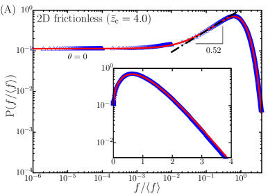
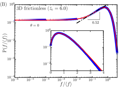
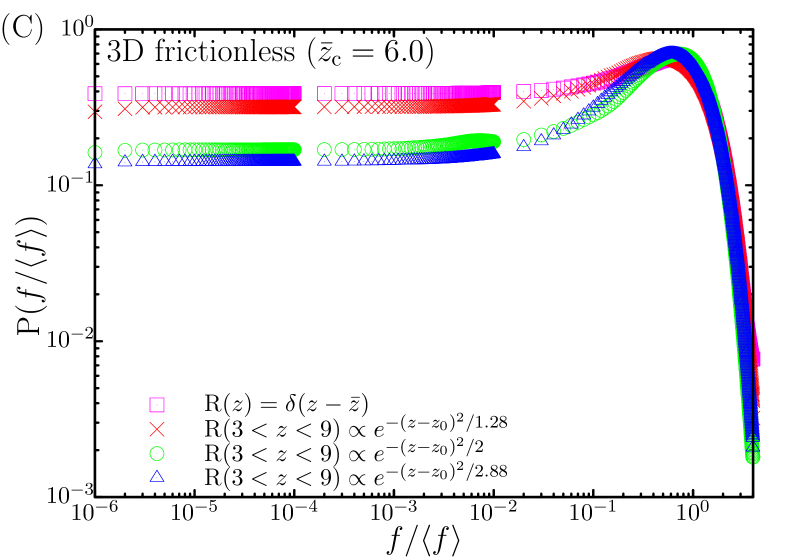
Figure 2: Force distribution, $\text{P}(f)$ in frictionless spheres packing in (A) 2-dimensional and (B) 3-dimensional systems. Results obtained from the cavity method (open triangles) show a flat regime (in a log-log plot) with exponent $\theta=0$ at small forces and $0.52$ in the intermediate region in both cases. We use here as a contact number distribution $\text{R}(3<z<9)\propto e^{-(z-z_{0})^{2}/2.88}$. In inset, log-linear plot of the same distribution exhibits approximate exponential tail at large forces. The red solid lines correspond to the fitting functions $P(x)$, as defined in the text. (C) Comparison of force distributions obtained with narrower distributions $\text{R}(z)$ (at fixed average $\bar{z}$). The exponent $\theta=0$ is obtained independently of the width of $\text{R}(z)$, but the peak in the force distribution becomes smaller when using a narrower $\text{R}(z)$.

We start by computing the force distribution ${\text{P}}(f=f^{\,n})$ for two and three-dimensional frictionless spheres packings, when we fix the average contact number ${\bar{z}}=\,{\bar{z}}_{\rm c}=4.0$ and $6.0$ respectively, by solving Eq. (15). Results in Fig. 2 reproduce the force distributions similar as seen in numerical simulations Radjai et al. (1996); O’Hern et al. (2001); Tkachenko and Witten (2000); Makse et al. (2000); Silbert et al. (2002); Zhang and Makse (2005); Donev et al. (2005); Lerner et al. (2013) and experiments Liu et al. (1995); Mueth et al. (1998); Løvoll et al. (1999); Erikson et al. (2002); Makse et al. (2000); Brujić et al. (2003, 2003). The force distribution we obtain can be well fitted with $P(x)=[7.84x^{2}+0.86-0.75/(1+4.10x)]e^{-2.67x}$ for 2-D (Fig. 2A) and $P(x)=[7.45x^{2}+1.20-1.06/(1+2.33x)]e^{-2.65x}$ for 3-D (Fig. 2B), with $x=f/\langle f\rangle$. Both fitting functions are close to the empirical fit $P(x)=[3.43x^{2}+1.45-1.18/(1+4.71x)]e^{-2.25x}$ to the force distribution of dense amorphous packings generated by Lubachevsky-Stillinger algorithm in 3-D by Donev et al. Donev et al. (2005). Note that although the tails of the force distributions can be well fitted to exponential, claims of the precise form of the tails are difficult to conclude, as the presented data only varies over $2$ decades.

Our method allows to access the small force region with unprecedented definition. We gather data down to $10^{-6}$ times the peak force (which is of the order of the pressure). This range is way below what is accessible with state of the art simulations of packings Radjai et al. (1996); O’Hern et al. (2001); Tkachenko and Witten (2000); Charbonneau et al. (2012); Silbert et al. (2002); Zhang and Makse (2005); Lerner et al. (2013). The reason for this is that we avoid two problems: (i) we work with Eq. (15) directly in the thermodynamic limit, whereas simulated packings typically are limited to few tens of thousands of forces Radjai et al. (1996); O’Hern et al. (2001); Tkachenko and Witten (2000); Silbert et al. (2002) which limits the definition of the obtained force distribution, and (ii) we can work exactly at the jamming transition point, as we set ${\bar{z}}=2D$, which contrasts with actual numerical or experimental studies where the limit of vanishing pressure with ${\bar{z}}=2D$ is very challenging.

The behavior of $\text{P}(f)$ at small forces has recently attracted attention Wyart (2012); Charbonneau et al. (2012); Lerner et al. (2013); DeGiuli et al. (2014), due to its central role for the mechanical stability of packings Wyart (2012); Lerner et al. (2013). Lerner et al. Lerner et al. (2013) pointed out a relation between the small force scaling $\text{P}(f)\sim f^{\theta}$ and the distribution function of the gaps $h$ between particles close to contact $g(h)\sim h^{-\gamma}$ via the inequality $\gamma\geq(1-\theta)/2$. Few empirical data exist so far for the $\theta$ exponent. Some recent efforts greatly improved the data statistics Charbonneau et al. (2012); Lerner et al. (2013); DeGiuli et al. (2014), but however still widely disagree over the value of the exponent, which is found anywhere between $\theta\approx 0.2$ and $\theta\approx 0.5$. This calls for more insight from theory.

Here we find for frictionless spheres a distribution of contact forces having a finite value for $f=0$ in the mean-field approximation. This translates as an exponent $\theta=0$ over four decades of data in both 2-D and 3-D packings (Fig. 2). We stress here that this observation is not dependent on the input distribution of coordination number $\text{R}(z)$. The comparison of the force distributions we obtain with various shapes of $\text{R}(z)$ is shown in Fig. 2C. In particular, the exponent $\theta=0$ as well as the large-force tail stays the same when we change $\text{R}(z)$ from the empirical fit $\text{R}(3<z<9)\propto e^{-(z-z_{0})^{2}/2.88}$ (at fixed average $\bar{z}$) to e.g. a regular graph $\text{R}(z)=\delta(z-\bar{z})$ in 3-D packings. However, the value of the exponent found in recent investigations Charbonneau et al. (2012); Lerner et al. (2013) seems to be incompatible with the value of $\theta$ obtained from our theory. The exponent might be dependent on the protocol by which jammed packings are generated Lerner et al. (2013), although this point is still debated DeGiuli et al. (2014). The value $\theta=0$ we obtain is an ensemble averaged, mean-field exponent. The value of the mean-field exponent might be lost in a finite-dimensional packing, but the fact that the exponent seems to be dimension independent Charbonneau et al. (2012) is an encouraging sign for a mean-field approach, as the mean-field value should be valid in high dimension. We note that a very recent work by Charbonneau et al. finds an exponent $\theta\approx 0.42$ in infinite dimensions from replica theory Kurchan et al. (2013); Charbonneau et al. (2013, 2014). Our exponent is incompatible with the relations $\gamma\geq 1/(2+\theta)$ derived by Wyart Wyart (2012), or $\gamma\geq(1-\theta)/2$ derived by Lerner et al Lerner et al. (2013), where $\gamma$ is the exponent describing the distribution function of the gaps $h$ between particles close to contact $g(h)\sim h^{-\gamma}$. Those two different relations are obtained from considerations of mechanical stability against respectively extended or local (buckling) excitations. In 3-D, the local excitations seem to be the dominant ones, and thus only the relation $\gamma\geq(1-\theta)/2$ should hold Lerner et al. (2013) in that case. In our mean-field framework, we miss the relation between excitation modes and force distribution because we neglect the spatial structure of finite dimensional packings. In fact, the pair correlation function in our framework has no structure beyond contact. Particle positions are omitted, apart from a local constraint of non overlaping, and there is therefore no excitation mode in our approach.

On the theoretical side, several values of $\theta$ have been predicted: the replica theory at the 1-RSB level also predicts a finite value for $\text{P}(f=0)$ Parisi and Zamponi (2010); Berthier et al. (2011); Charbonneau et al. (2012) (it predicts a Gaussian for $\text{P}(f)$), but the fullRSB solution gives $\theta\approx 0.42$ in infinite dimensions Kurchan et al. (2013); Charbonneau et al. (2013, 2014); the q-model can give several values for $\theta$, depending on the underlying assumptions, but in any case predicts $\theta\geq 1$ Liu et al. (1995); Coppersmith et al. (1996); and Edwards’ model predicts $\theta=1/({\bar{z}}-2)$ Brujić et al. (2003, 2003). The differences between Edwards’ and q-model approaches, which mostly stem from the treatment of local disorder in the contact normal directions, indicate that the way to deal with this disorder is crucial for a correct description of the small force behavior.

Interestingly, we find an intermediate regime for $f$ slightly smaller than its average value $\langle f\rangle$, for which $\text{P}(f)\sim f^{0.52}$ (Fig. 2A, Fig. 2B). We observe that this pseudo-exponent gets smaller when using a narrower $\text{R}(z)$ as input (Fig. 2C). The smallest value it can reach for regular graph $\text{R}(z)=\delta(z-\bar{z})$ are $\sim 0.40$ in 2-D and $\sim 0.21$ in 3-D packings respectively. The results of this regime, extending from $f\simeq 10^{-2}\langle f\rangle$ to $f\simeq\langle f\rangle$ is the one probed by most experiments and simulations. This suggests that careful measurements at very small $f$ are needed to avoid pre-asymptotic behavior in the estimation of $\theta$ from experimental or numerical data, which might explain a lot of discrepancies observed in the current literature. Only few very recent numerical data managed to reach this regime Lerner et al. (2013); DeGiuli et al. (2014).

III.2 Calculation of $\,{\bar{z}}_{\rm c}^{\rm min}(\mu)$ for sphere packings with arbitrary friction coefficient

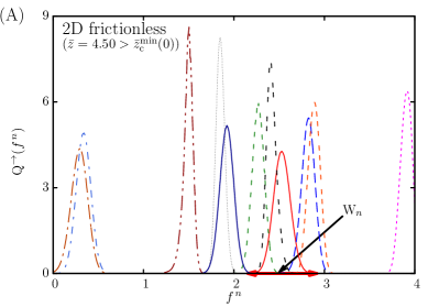
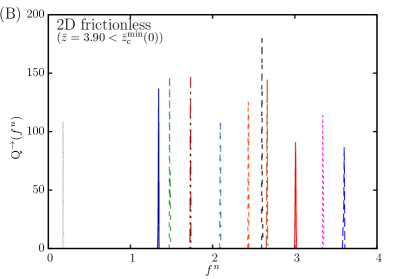
Figure 3: The force distribution $\{\text{Q}^{\to}(f^{\,n})\}$ when (A) $\bar{z}=4.50>\,{\bar{z}}_{\rm c}^{\rm min}(0)$ and (B) when $\bar{z}=3.90<\,{\bar{z}}_{\rm c}^{\rm min}(0)$ for 2-D frictionless spheres packing. In (A), the ‘width’ of $\text{Q}^{\to}(f^{\,n})$ on $f^{\,n}$ is defined by $\text{W}_{n}$ as the difference of two extreme values of $f^{\,n}$ at which $\text{Q}^{\to}(f^{\,n})$ is equal to $10^{-3}$.

We turn to the determination of the force distribution for arbitrary friction coefficient $\mu$ and a lower bound on $\,{\bar{z}}_{\rm c}$ for the existence of random packings of spheres at a given $\mu$. This threshold corresponds to the point where solutions of the cavity equations Eq. (6) and Eq. (8) no longer exist.

We search for the existence of a solution by applying the Population Dynamics algorithm described in section II.2. A solution exists if this process leads to a converged averaged width of the distributions of the population $\{\text{Q}^{\to}\}$ used to describe $\mathcal{Q}(\text{Q}^{\to})$. Even though this algorithm does not require a very large population (as we do not seek to obtain a detailed description of $\mathcal{Q}(\text{Q}^{\to})$ and only want to know if it exists), its computational cost is still high, and we here apply the method to frictionless packings and 2-D frictional packings only.

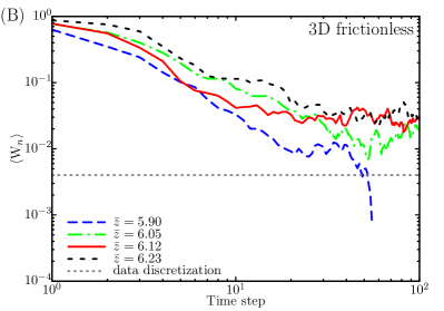
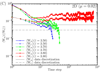
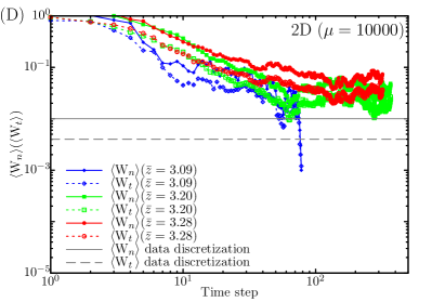
Figure 4: (A) Evolution of average width $\langle\text{W}_{n}\rangle$ (and $\langle\text{W}_{t}\rangle$ if frictional) of a large population $\{\text{Q}^{\to}\}$ versus time step in population dynamics in (A) 2-D frictionless, (B) 3-D frictionless, (C) 2-D frictional packing with $\mu=0.02$ and (D) 2-D frictional packing with $\mu=10000$. $\,{\bar{z}}_{\rm c}^{\rm min}(\mu)$ is found at (A) $\,{\bar{z}}_{\rm c}^{\rm min}(\mu=0)\in[3.94,4.02]$ in 2-D frictionless spheres packing, (B) $\,{\bar{z}}_{\rm c}^{\rm min}(\mu=0)\in[5.90,6.05]$ in 3-D frictionless spheres packing, (C) $\,{\bar{z}}_{\rm c}^{\rm min}(\mu=0.02)\in[3.70,3.80]$ and (D) $\,{\bar{z}}_{\rm c}^{\rm min}(\mu=10000)\in[3.09,3.20]$ in 2-D frictional spheres packing.

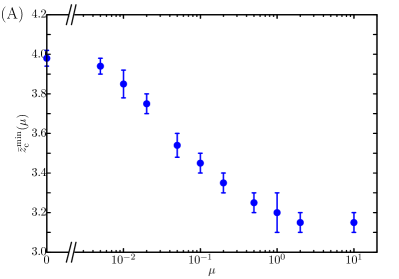
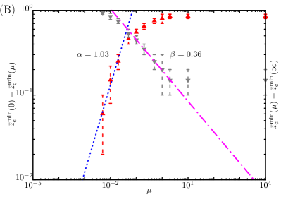
Figure 5: (A) Linear-Log plot of the full curve $\,{\bar{z}}_{\rm c}^{\rm min}(\mu)$ vs. $\mu$ for various friction coefficients in 2-D spheres packing. $\,{\bar{z}}_{\rm c}^{\rm min}(\mu)$ shows a monotonic decrease with increasing $\mu$ from $\,{\bar{z}}_{\rm c}^{\rm min}({\mu=0})=2D=4$ to $\,{\bar{z}}_{\rm c}^{\rm min}({\mu=\infty})\gtrsim D+1=3$. Error bar indicates the range from the largest $\,{\bar{z}}_{\rm c}^{\rm min}(\mu)$ having no solution to the smallest $\,{\bar{z}}_{\rm c}^{\rm min}(\mu)$ having solution. Data point represents the mean of the range. (B) Two power law scaling relations $\,{\bar{z}}_{\rm c}^{\rm min}(0)-\,{\bar{z}}_{\rm c}^{\rm min}({\mu})\sim{\mu}^{\alpha}$, $\,{\bar{z}}_{\rm c}^{\rm min}({\mu})-\,{\bar{z}}_{\rm c}^{\rm min}({\infty})\sim{\mu}^{-\beta}$ are found with $\alpha=1.03$, $\beta=0.36$, respectively.

For frictionless packings, the ‘width’ of a force distribution $\text{Q}^{\to}(f^{n})$, denoted by $\text{W}_{n}$, is defined as the difference of two extreme values of $f^{n}$ at which $\text{Q}^{\to}(f^{n})$ is equal to $10^{-3}$ (see Fig. 3A). To determine the existence of solution, we calculate the average width over the sites as $\langle\text{W}_{n}\rangle$. Fig. 4A shows the evolution of the average width of distributions at different $\bar{z}$ versus time step in population dynamics for the particular case of 2-D frictionless spheres packings. Results indicate that the final population of distributions $\{\text{Q}^{\to}\}$ after $t_{\rm max}$ iterations have dramatically different shapes at various $\bar{z}$. We find that the population $\{\text{Q}^{\to}\}$ rapidly tends to a set of non-overlapping Dirac peaks when $\bar{z}$ is small (shown in Fig. 3B for $\bar{z}=3.90$). In this case, the average width of fields decreases as a function of time step in the Population Dynamics iteration and finally goes below data discretization (the interval of force to integrate the force distribution), leading to no solution of $\text{Q}^{i}(f^{\,n})$ according to Eq. (5). Thus the system is overdetermined in the sense that $\bar{z}$ contacts per particle are not enough to stabilize the whole packing. In contrast, when $\bar{z}$ is increased (shown in Fig. 3A for $\bar{z}=4.50$), the distributions in $\{\text{Q}^{\to}\}$ become broad. The average width converges to a finite value as seen in Fig. 4A, allowing a non-vanishing force distribution $\text{Q}^{i}(f^{\,n})$ at each contact. In this case a set of solutions to force and torque balances exists. The range between the largest $\bar{z}$ having no solution and the smallest $\bar{z}$ having solution is the range where $\,{\bar{z}}_{\rm c}^{\rm min}(\mu)$ belongs to. In addition to 2-D frictionless packings, result of 3-D frictionless packings is shown in Fig. 4B. The transition points $\,{\bar{z}}_{\rm c}^{\rm min}(\mu=0)=2D$ are found in the expected range for both 2-D and 3-D frictionless packings.

For frictional packings, the force distribution $\text{Q}^{\to}(f^{\,n},f^{\,t})$ has the shape of a ‘blob’ that spreads on the $f^{\,n},f^{\,t}$-plane. In this case the width of the force distribution $\text{W}_{n}$ and $\text{W}_{t}$ are defined as the width of the spread from side to side on axis $f^{\,n}$ and $f^{\,t}$ respectively with $\text{Q}^{\to}(f^{\,n},f^{\,t})$ higher than $10^{-3}$: e.g. $\text{W}_{n}=f^{\,n}_{\text{max}}-f^{\,n}_{\text{min}}$, where $f^{\,n}_{\text{max}}$ is the smallest value satisfies the condition $\text{Q}^{\to}(f^{\,n}>f^{\,n}_{\text{max}},f^{\,t})<10^{-3}$ and $f^{\,n}_{\text{min}}$ is the largest value satisfies the condition $\text{Q}^{\to}(f^{\,n}<f^{\,n}_{\text{min}},f^{\,t})<10^{-3}$. Here we obtain data of average width $\langle\text{W}_{n}\rangle$ and $\langle\text{W}_{t}\rangle$ of distributions $\{\text{Q}^{\to}\}$ in 2-D frictional spheres packings with arbitrary friction coefficient. Similarly, the force distributions have different shapes after $t_{\rm max}$ iterations, from which we determine, for example, the satisfiability transition point of force and torque balances in 2-D spheres packing at $\,{\bar{z}}_{\rm c}^{\rm min}(0.02)\in[3.70,3.80]$ (Fig. 4C) and $\,{\bar{z}}_{\rm c}^{\rm min}(10000)\in[3.09,3.20]$ (Fig. 4D). The full curve $\,{\bar{z}}_{\rm c}^{\rm min}(\mu)$ is shown in Fig. 5A for 2-D frictional spheres packing. We observe a monotonic decrease with increasing $\mu$ from $2D=4$ at $\mu=0$, a well-known behavior of frictional packings, previously found in numerous studies, both experimentally and numerically Snoeijer et al. (2004); Moukarzel (1998); Silbert et al. (2002, 2002); Zhang and Makse (2005); Shundyak et al. (2007); Song et al. (2008); Wang et al. (2010); Silbert (2010); Papanikolaou et al. (2013). Notice that the critical contact number we obtain at infinite friction is slightly above the Maxwell argument $D+1$; also a typical feature Silbert et al. (2002); Shundyak et al. (2007); Wang et al. (2010). This is interesting, as it means that the naive counting argument, ignoring the repulsive nature of the forces, fails to reproduce the correct bound for such a simple case as sphere packings with $\mu\to\infty$, where neither Coulomb condition nor non-trivial geometrical features complexify the picture. The fact that the naive Maxwell counting argument still gives the correct bound for frictionless sphere packing can therefore be seen as a quite fortunate isolated prediction. In Fig. 5B, two power law scaling relations $\,{\bar{z}}_{\rm c}^{\rm min}(0)-\,{\bar{z}}_{\rm c}^{\rm min}(\mu)\sim{\mu}^{\alpha},\,{\bar{z}}_{\rm c}^{\rm min}(\mu)-\,{\bar{z}}_{\rm c}^{\rm min}(\infty)\sim{\mu}^{-\beta}$ are found with $\alpha=1.03$, $\beta=0.36$ respectively. Our result $\alpha$ agrees well with the prediction of 2-D monodisperse packing $\alpha=1$ by Wang et al Wang et al. (2010), and is not far away from previous simulation of 2-D polydisperse packings $\alpha=0.70$ Shundyak et al. (2007), while $\beta$ is much smaller than their predicted value $\beta=2$ and the result of $\beta=1.86$ obtained from simulation Wang et al. (2010).

III.3 Joint force distribution for frictional spheres packings

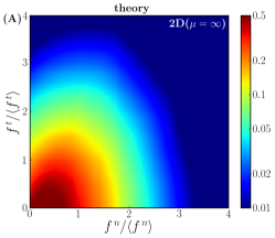
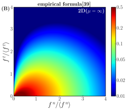
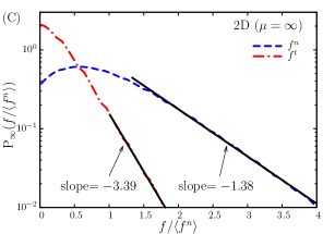
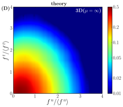
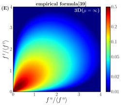
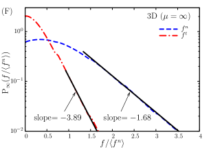
Figure 6: Theory and Simulations. The joint force distribution $\text{P}_{\mu}(f^{\,n},f^{\,t})$ from theoretical calculation in (A) 2-D spheres packing with $\mu=\infty$, and in (D) 3-D spheres packing with $\mu=\infty$. The contour plots of the empirical formula $\text{P}_{\infty}(f,\theta)=ag(\theta)\exp{(-\sqrt{a}f)}$ with $a=0.8$ which was previously found by Wang et al Wang et al. (2010) are shown in (B) and (E) for 2-D and 3-D respectively. Plots of the corresponding probability distribution of normalized normal forces and frictional forces in 2-D and 3-D are shown in (C) and (F) respectively.

Similar to the frictionless case, the cavity method can generate the joint force distribution $\text{P}_{\mu}(f^{\,n},f^{\,t})$ for frictional spheres packings with friction coefficient $\mu$. The simplest case of infinite friction, $\text{P}_{\mu=\infty}(f^{\,n},f^{\,t})$ for 2-D and 3-D sphere packings are shown in Fig. 6A and Fig. 6D respectively, and results follow similar behavior as the empirical fitting formula $\text{P}_{\infty}(f,\theta)=ag(\theta)\exp{(-\sqrt{a}f)}$, (where $g(\theta)=(D-1)(\sin{\theta})^{D-2}\cos{\theta}$, $f\!\!\!=\!\!\!\sqrt{(f^{\,n})^{2}+(f^{\,t})^{2}}$, $\theta\!=\!\arctan{(\frac{f^{\,t}}{f^{\,n}})}$ and $a=0.8$) measured in previous numerical studies Wang et al. (2010) (Fig. 6B and Fig. 6E). In particular, we recover the non-trivial qualitative change between 2-D and 3-D Wang et al. (2010): while in 3-D, $\text{P}_{\mu=\infty}(f^{\,n},f^{\,t})\simeq\text{P}_{\mu=\infty}(f^{\,t},f^{\,n})$, in 2-D, this symmetry is clearly broken. This is a consequence of the more symmetrical role tangential and normal forces play in 3-D with as many torque balance as force balance equations, whereas in 2-D, there are twice less torque balance than force balance equations. When the friction coefficient is finite (see Fig. 7A), the pattern inside the Coulomb cone looks similar to the one obtained at infinite friction. Quite interestingly, we do not observe any excess of forces at the Coulomb threshold $f^{\,t}=\mu f^{\,n}$, implying that there are no sliding contacts. This offers a theoretical explanation to a singular fact already observed in simulations: control parameters (essentially volume fraction and friction coefficient) being equal, the percentage of plastic contacts in a packing depends on the preparation protocol Zhang and Makse (2005); Atman et al. (2013). Our formalism takes into account those different packings (hence protocols) by performing a statistical average over possible packings, and the outcome shows that packings without plastic contacts are dominant. In this regards, the fragility associated with the large number of plastic contacts in many experimentally or numerically generated packings could be mostly attributed to the preparation protocol, rather than to an inherent property of random packings of frictional spheres.

Furthermore, we obtain the distributions of the normal and tangential components for frictionless and frictional packings as plotted in Fig. 6C, Fig. 6F and Fig. 7B. The normal force distributions all have slight peaks around the mean and approximate exponential tails at large forces. Below the mean, the normal force distribution for infinite friction has a nonzero probability at zero force whereas it shows a dip towards zero for $\mu=0.2$. The tangential force distribution also has an approximate exponential tail, however, it decreases monotonically without an obvious rise at small forces. Our results of the probability distribution of normal forces and tangential forces agree with previous experimental measurements in 2-D frictional spheres packing Majmudar and Behringer (2005).

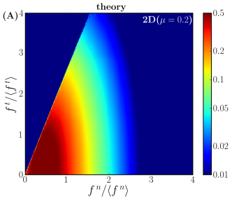
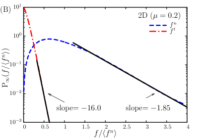
Figure 7: (A) The joint force distribution $\text{P}_{0.2}(f^{\,n},f^{\,t})$ with friction coefficient $\mu=0.2$ in 2-D spheres packing. (B) Plots of the probability distribution of normalized normal forces and frictional forces.

IV Discussion and Conclusion

In conclusion, we develop a theoretical framework by using the cavity method, introduced initially for the study of spin-glasses and optimization problems, to obtain a statistical physics mean-field description of the force and torque balances constraints in a random packing. This allows us to get the force distribution and the lower bound on the average coordination number in frictional and frictionless spheres packings.

We find a mean-field signature of jamming in the finite value $\text{P}(f=0)$ of the force distribution at small force. We also notice that there is a power law rise $\text{P}(f)\sim f^{0.52}$ in the intermediate region of $\text{P}(f)$. Thus it is likely that one obtains an exponent $0<\theta<0.52$ if the simulations or experiments can not achieve data down to low enough forces. However, we must stress that the mean-field approach we develop does not include the detailed structure of finite dimensional systems, which may have an important effect on the $\theta$ exponent. Indeed some recent data seem to extend beyond the intermediate regime $\text{P}(f)\sim f^{0.52}$ and find a finite exponent at small force Charbonneau et al. (2012); Lerner et al. (2013). For frictional packings, we can access the complete joint distribution $\text{P}_{\mu}(f^{\,n},f^{\,t})$.

Concerning the average coordination number, we describe its lower bound $\,{\bar{z}}_{\rm c}^{\rm min}(\mu)$, which interpolates smoothly between the isostatic frictionless case $\,{\bar{z}}_{\rm c}^{\rm min}(0)=2D$, and a large $\mu$ limit $\,{\bar{z}}_{\rm c}^{\rm min}(\infty)$ slightly above $D+1$. This confirms that there is no discontinuity at $\mu=0$. We predict two scalings for small and large friction coefficients as $\,{\bar{z}}_{\rm c}^{\rm min}(0)-\,{\bar{z}}_{\rm c}^{\rm min}(\mu)\sim{\mu}^{1.03}$ and $\,{\bar{z}}_{\rm c}^{\rm min}(\mu)-\,{\bar{z}}_{\rm c}^{\rm min}(\infty)\sim{\mu}^{-0.36}$.

The statistical mechanics point of view on force and torque balances for random packings thus proves fruitful. Many features of these systems can be inferred from those simple considerations. The use of the cavity technique enables us to tackle this problem with a correct treatment of the disorder, leading to several new results. This formalism will be extended to packings of more general shapes and could be used to predict other properties of disordered packings, like the yield stress for instance. Granular materials are not the only systems subject to force and torque balances, and this constraint is seen in all overdamped systems, among which suspensions at low Reynolds number constitute an important example, both conceptually and practically. We hope that our results will motivate investigations in this direction.

Appendix: Statistical physics description

Here we give the statistical physics description of the packing problem motivating the definition of the partition function $Z$ in Eq. (3) of the main text.

We define for a given contact network $G$, of $N$ particles and $M$ forces $\vec{f}^{\,a}_{i}=-f_{i}^{\,n}\hat{n}^{\,a}_{i}+f_{i}^{\,t}\hat{t}^{\,a}_{i}$ exerted on particle $a$ at position $\vec{r}_{i}^{\,a}$ (with respect to the center of the particle), an energy function which is the sum of the square of total forces and torques on each particle,

$$H=\sum^{N}_{a=1}\Big{(}\sum_{i\in\partial a}\vec{f}_{i}^{\,a}\Big{)}^{2}+\sum^{N}_{a=1}\Big{(}\sum_{i\in\partial a}\vec{r}_{i}^{\,a}\times\vec{f}_{i}^{\,a}\Big{)}^{2}+\Big{(}\sum_{i=1}^{M}f_{i}^{\,n}-Mp\Big{)}^{2}.$$ (16)

We then define the partition function of contact network $G$ with quenched disorder on the contact normals $\{\hat{n}^{\,a}_{i}\}$,

$$\begin{array}[]{rl}Z_{\beta}=&\!\!\!\displaystyle\int\prod_{i=1}^{M}\Big{[}\,\text{d}f_{i}^{\,n}\,\text{d}f_{i}^{\,t}\,\text{d}\hat{t}^{\,a}_{i}\,\text{d}\hat{t}^{\,b}_{i}\,\delta(\hat{t}^{\,a}_{i}+\hat{t}^{\,b}_{i})\\ &\qquad\qquad\qquad\displaystyle\Theta(f_{i}^{\,n})\Theta(\mu f_{i}^{\,n}-f_{i}^{\,t})\Big{]}\mathrm{e}^{-\beta H},\end{array}$$ (17)

where $\beta$ is an inverse temperature, which is only here as a parameter (it is not the actual temperature, which is irrelevant for granular packings), and will be set to $\beta\to\infty$ soon. The Heaviside $\Theta$ functions ensure repulsive normal forces, and Coulomb friction condition, respectively.

The ground state of the hamiltonian $H$ at $\beta\to\infty$ provides the balance condition in the packing. Consider the repulsive nature of contact forces and the Coulomb condition when friction exists, by using the factor graph representation of the Boltzmann probability, the weight of interaction node $a$ (a particle on which force/torque balance is satisfied) is

$$\begin{array}[]{rl}&\hskip-14.45377pt\chi_{a}^{\beta}(\{f^{\,n},f^{\,t},\hat{n}^{\,a},\hat{t}^{\,a}\}_{\partial a})\displaystyle=\frac{1}{Z^{\,a}_{\beta}}\exp\Big{[}-\beta\big{(}\displaystyle\sum_{i\in\partial a}\vec{f}_{i}^{\,a}\big{)}^{2}\\ &-\beta\big{(}\displaystyle\sum_{i\in\partial a}\vec{r}_{i}^{\,a}\times\vec{f}_{i}^{\,a}\big{)}^{2}\Big{]}\displaystyle\prod_{i\in\partial a}\Theta(f_{i}^{\,n})\Theta(\mu f_{i}^{\,n}-f_{i}^{\,n}),\end{array}$$ (18)

with $Z^{\,a}_{\beta}$ ensuring

$$1=\int\prod_{i\in\partial a}\,\text{d}f_{i}^{\,n}\,\text{d}f_{i}^{\,t}\,\text{d}\hat{t}^{\,a}_{i}\chi_{a}^{\beta}(\{f^{\,n},f^{\,t},\hat{n}^{\,a},\hat{t}^{\,a}\}_{\partial a}).$$

In the zero temperature limit $\beta\to\infty$, the above expression becomes the force/torque balance constraint on each node:

$$\begin{array}[]{rl}&\hskip-14.45377pt\chi_{a}(f)=\displaystyle\lim_{\beta\to\infty}\chi_{a}^{\beta}(f)\\ &\hskip-7.22743pt=\delta\Big{(}\displaystyle\sum_{i\in\partial a}\vec{f}_{i}^{\,a}\Big{)}\delta\Big{(}\displaystyle\sum_{i\in\partial a}\vec{r}_{i}^{\,a}\times\vec{f}_{i}^{\,a}\Big{)}\displaystyle\prod_{i\in\partial a}\Theta(f_{i}^{\,n})\Theta(\mu f_{i}^{\,n}-f_{i}^{\,t}),\end{array}$$ (19)

Notice that in this limit the exact shape of hamiltonian Eq. (16) is irrelevant, as its only condition is that it provides the force and torque balances in the limiting case $\beta\to\infty$.

The associated partition function $Z=\lim_{\beta\to\infty}Z_{\beta}$ is then the one defined in Eq. (3) of the main text. This partition function is defined at the level of a single graph, but we study the problem for an ensemble of random graphs, ie we average the entropy $\log Z$ over the selected ensemble of random graphs, defined by the distribution of connectivity (contact number) $\mathrm{R}(z)$ and the joint probability distribution of the contact directions $\Omega(\{\hat{n}\})$ around every interaction node (particle), as explained in the main text. This ensemble is .

References

- Behringer and Jenkins (1997) R. P. Behringer and J. T. Jenkins, Powders & Grains 97: Proceedings of the Third International Conference on Powders & Grains, Durham, North Carolina, 18-23 May 1997, Balkema, 1997.
- Zhou et al. (2006) J. Zhou, S. Long, Q. Wang and A. D. Dinsmore, Science, 2006, 312, 1631–1633.
- Liu et al. (1995) C. h. Liu, S. R. Nagel, D. A. Schecter, S. N. Coppersmith, S. Majumdar, O. Narayan and T. A. Witten, Science, 1995, 269, 513–515.
- Mueth et al. (1998) D. M. Mueth, H. M. Jaeger and S. R. Nagel, Phys. Rev. E, 1998, 57, 3164–3169.
- Løvoll et al. (1999) G. Løvoll, K. J. Måløy and E. G. Flekkøy, Phys. Rev. E, 1999, 60, 5872–5878.
- Erikson et al. (2002) J. M. Erikson, N. W. Mueggenburg, H. M. Jaeger and S. R. Nagel, Phys. Rev. E, 2002, 66, 040301.
- Brujić et al. (2003) J. Brujić, S. F Edwards, I. Hopkinson and H. A. Makse, Phys. A, 2003, 327, 201–212.
- Brujić et al. (2003) J. Brujić, S. F. Edwards, D. V. Grinev, I. Hopkinson, D. Brujić and H. A. Makse, Faraday Discuss., 2003, 123, 207–220.
- Radjai et al. (1996) F. Radjai, M. Jean, J.-J. Moreau and S. Roux, Phys. Rev. Lett., 1996, 77, 274–277.
- O’Hern et al. (2001) C. S. O’Hern, S. A. Langer, A. J. Liu and S. R. Nagel, Phys. Rev. Lett., 2001, 86, 111–114.
- Tkachenko and Witten (2000) A. V. Tkachenko and T. A. Witten, Phys. Rev. E, 2000, 62, 2510–2516.
- Makse et al. (2000) H. A. Makse, D. L. Johnson and L. M. Schwartz, Phys. Rev. Lett., 2000, 84, 4160–4163.
- Wyart (2012) M. Wyart, Phys. Rev. Lett., 2012, 109, 125502.
- Lerner et al. (2013) E. Lerner, G. Düring and M. Wyart, Soft Matter, 2013, 9, 8252–8263.
- Coppersmith et al. (1996) S. N. Coppersmith, C. h. Liu, S. Majumdar, O. Narayan and T. A. Witten, Phys. Rev. E, 1996, 53, 4673–4685.
- Socolar (1998) J. E. Socolar, Phys. Rev. E, 1998, 57, 3204.
- Charbonneau et al. (2012) P. Charbonneau, E. I. Corwin, G. Parisi and F. Zamponi, Phys. Rev. Lett., 2012, 109, 205501.
- Kurchan et al. (2013) J. Kurchan, G. Parisi, P. Urbani and F. Zamponi, J. Phys. Chem. B, 2013, 117, 12979–12994.
- Charbonneau et al. (2013) P. Charbonneau, J. Kurchan, G. Parisi, P. Urbani and F. Zamponi, arXiv:1310.2549 [cond-mat], 2013.
- Charbonneau et al. (2014) P. Charbonneau, J. Kurchan, G. Parisi, P. Urbani and F. Zamponi, Nat. Commun., 2014, 5, 3725.
- Edwards and Oakeshott (1989) S. F. Edwards and R. Oakeshott, Phys. A, 1989, 157, 1080–1090.
- Kruyt and Rothenburg (2002) N. Kruyt and L. Rothenburg, Int. J. Solids Struct., 2002, 39, 571–583.
- Bagi (2003) K. Bagi, Granul. Matter, 2003, 5, 45–54.
- Goddard (2004) J. Goddard, Int. J. Solids Struct., 2004, 41, 5851 – 5861.
- Henkes and Chakraborty (2009) S. Henkes and B. Chakraborty, Phys. Rev. E, 2009, 79, 061301.
- Snoeijer et al. (2004) J. H. Snoeijer, T. J. H. Vlugt, M. van Hecke and W. van Saarloos, Phys. Rev. Lett., 2004, 92, 054302.
- Tighe et al. (2008) B. P. Tighe, A. R. T. van Eerd and T. J. H. Vlugt, Phys. Rev. Lett., 2008, 100, 238001.
- van Eerd et al. (2007) A. R. van Eerd, W. G. Ellenbroek, M. van Hecke, J. H. Snoeijer and T. J. Vlugt, Phys. Rev. E, 2007, 75, 060302.
- Parisi and Zamponi (2010) G. Parisi and F. Zamponi, Rev. Mod. Phys., 2010, 82, 789–845.
- Berthier et al. (2011) L. Berthier, H. Jacquin and F. Zamponi, Phys. Rev. E, 2011, 84, 051103.
- Majmudar and Behringer (2005) T. S. Majmudar and R. P. Behringer, Nature, 2005, 435, 1079–1082.
- Lerner et al. (2012) E. Lerner, G. Düring and M. Wyart, Europhys. Lett., 2012, 99, 58003.
- Alexander (1998) S. Alexander, Phys. Rep., 1998, 296, 65 – 236.
- Tkachenko and Witten (1999) A. V. Tkachenko and T. A. Witten, Phys. Rev. E, 1999, 60, 687–696.
- Moukarzel (1998) C. F. Moukarzel, Phys. Rev. Lett., 1998, 81, 1634–1637.
- Maxwell (1864) J. C. Maxwell, Philos. Mag., 1864, 27, 294–299.
- Silbert et al. (2002) L. E. Silbert, D. Ertaş, G. S. Grest, T. C. Halsey and D. Levine, Phys. Rev. E, 2002, 65, 031304.
- Silbert et al. (2002) L. E. Silbert, G. S. Grest and J. W. Landry, Phys. Rev. E, 2002, 66, 061303.
- Zhang and Makse (2005) H. P. Zhang and H. A. Makse, Phys. Rev. E, 2005, 72, 011301.
- Shundyak et al. (2007) K. Shundyak, M. van Hecke and W. van Saarloos, Phys. Rev. E, 2007, 75, 010301.
- Song et al. (2008) C. Song, P. Wang and H. A. Makse, Nature, 2008, 453, 629–632.
- Wang et al. (2010) P. Wang, C. Song, C. Briscoe, K. Wang and H. A. Makse, Phys. A, 2010, 389, 3972 – 3977.
- Silbert (2010) L. E. Silbert, Soft Matter, 2010, 6, 2918–2924.
- Papanikolaou et al. (2013) S. Papanikolaou, C. S. O’Hern and M. D. Shattuck, Phys. Rev. Lett., 2013, 110, 198002.
- Brujić et al. (2007) J. Brujić, C. Song, P. Wang, C. Briscoe, G. Marty and H. A. Makse, Phys. Rev. Lett., 2007, 98, 248001.
- M. Mezard and Virasoro (1986) G. P. M. Mezard and M. A. Virasoro, Spin Glass Theory And Beyond, World Scientific, Singapore, 1986.
- O’Hern et al. (2003) C. S. O’Hern, L. E. Silbert, A. J. Liu and S. R. Nagel, Phys. Rev. E, 2003, 68, 011306.
- Mezard and Montanari (2009) M. Mezard and A. Montanari, Information, Physics, and Computation, Oxford University Press, USA, 2009.
- Edwards and Grinev (1999) S. F. Edwards and D. V. Grinev, Phys. Rev. Lett., 1999, 82, 5397–5400.
- Henkes et al. (2010) S. Henkes, K. Shundyak, W. v. Saarloos and M. v. Hecke, Soft Matter, 2010, 6, 2935–2938.
- Wang et al. (2010) P. Wang, C. Song, Y. Jin, K. Wang and H. A. Makse, J. Stat. Mech. Theor. Exp., 2010, 2010, P12005.
- Makse et al. (2004) H. A. Makse, J. Brujić and S. F. Edwards, “Statistical mechanics of jammed matter”, The Physics of Granular Media, Wiley, New York, 2004, pp. 45–86.
- Press et al. (2007) W. H. Press, S. A. Teukolsky, W. T. Vetterling and B. P. Flannery, “Section 2.10. QR Decomposition”, Numerical Recipes: The Art of Scientific Computing, Cambridge University Press, New York, NY, USA, 3rd edn, 2007.
- Donev et al. (2005) A. Donev, S. Torquato and F. H. Stillinger, Phys. Rev. E, 2005, 71, 011105.
- DeGiuli et al. (2014) E. DeGiuli, E. Lerner, C. Brito and M. Wyart, arXiv:1402.3834 [cond-mat], 2014.
- Atman et al. (2013) A. P. F. Atman, P. Claudin, G. Combe and R. Mari, Europhys. Lett., 2013, 101, 44006.