Multilevel Monte Carlo for random degenerate scalar convection diffusion equation

Abstract.

We consider the numerical solution of scalar, nonlinear degenerate convection-diffusion problems with random diffusion coefficient and with random flux functions. Building on recent results on the existence, uniqueness and continuous dependence of weak solutions on data in the deterministic case, we develop a definition of random entropy solution. We establish existence, uniqueness, measurability and integrability results for these random entropy solutions, generalizing [28, 29] to possibly degenerate hyperbolic-parabolic problems with random data. We next address the numerical approximation of random entropy solutions, specifically the approximation of the deterministic first and second order statistics. To this end, we consider explicit and implicit time discretization and Finite Difference methods in space, and single as well as Multi-Level Monte-Carlo methods to sample the statistics. We establish convergence rate estimates with respect to the discretization parameters, as well as with respect to the overall work, indicating substantial gains in efficiency are afforded under realistic regularity assumptions by the use of the Multi-Level Monte-Carlo method. Numerical experiments are presented which confirm the theoretical convergence estimates.

1. Introduction

Many problems in physics and engineering are modeled by nonlinear, possibly strongly degenerate, convection diffusion equation. The Cauchy problem for such equations takes the form

(1.1) $$\begin{cases}u_{t}+\operatorname*{div}f(u)=\Delta A(u),&(x,t)\in\Pi_{T},\\ u(0,x)=u_{0}(x),&x\in\mathbb{R}^{d},\end{cases}$$

where $\Pi_{T}=\mathbb{R}^{d}\times(0,T)$ with $T>0$ fixed, $u:\Pi_{T}\to\mathbb{R}$ is the unknown function, $f=(f_{1},\ldots,f_{d})$ the flux function, and $A$ the nonlinear diffusion. Regarding this, the basic assumption is that $a(u):=A^{\prime}(u)\geq 0$ for all $u$. When (1.1) is nondegenerate, i.e., $a(u)>0$, it is well known that (1.1) admits a unique classical solution [34]. This contrasts with the degenerate case where $a(u)$ may vanish for some values of $u$. A simple example of a degenerate equation is the porous medium equation

$$u_{t}=\Delta(u^{m}),\ m>1,$$

which degenerates at $u=0$. This equation has served as a simple model to describe processes involving fluid flow, heat transfer or diffusion. Examples of applications are in the description of the flow of an isentropic gas through a porous medium, modelled by Leibenzon [27] and Muskat [32] around 1930, in the study of groundwater flow by Boussisnesq in 1903 [3] or in heat radiation in plasmas, Zel’dovich and collaborators around 1950, [38]. In general, a manifestation of the degeneracy in (1.1) is the finite speed of propagation of disturbances. If $a(0)=0$, and if at some fixed time the solution $u$ has compact support, then it will continue to have compact support for all later times.

By the term “strongly degenerate” we mean that there is an open interval such that $a(u)=0$ if $u$ is in this interval. Hence, the class of equations under consideration is very large and contains the heat equation, the porous medium equation and scalar conservation laws. Independently of the smoothness of the initial data, due to the degeneracy of the diffusion, singularities may form in the solution $u$. Therefore we consider weak solutions which are defined as follows.

Definition 1.1.

Set $\Pi_{T}=\mathbb{R}^{d}\times(0,T)$. A function

$$u(t,x)\in C\left([0,T];L^{1}(\mathbb{R}^{d})\right)\cap L^{\infty}(\Pi_{T})$$

is a weak solution of the initial value problem (1.1) if it satisfies:

1. $\operatorname*{grad}A(u)\in L^{\infty}(\Pi_{T})$.

2. For all test functions $\varphi\in\mathcal{D}(\mathbb{R}^{d}\times[0,T))$

   (1.2) $$\iint_{\Pi_{T}}\left(u\varphi_{t}+f(u)\cdot\operatorname*{grad}\varphi+A(u)\Delta\varphi\right)\,dx\,dt+\int_{\mathbb{R}^{d}}u_{0}(x)\varphi(x,0)\,dx=0.$$

In view of the existence theory, the condition D.1 is natural, and thanks to this we can replace (1.2) by

$$\iint_{\Pi_{T}}u\varphi_{t}+\left(f(u)-\operatorname*{grad}A(u)\right)\cdot\operatorname*{grad}\varphi\,dxdt+\int_{\mathbb{R}^{d}}u_{0}(x)\varphi(x,0)\,dx=0.$$

If $A$ is constant on a whole interval, then weak solutions are not uniquely determined by their initial data, and one must impose an additional entropy condition to single out the physically relevant solution. A weak solution satisfies the entropy condition if

(1.3) $$\varrho(u)_{t}+\operatorname*{div}q(u)-\Delta r(u)\leq 0\ \text{in $\mathcal{D}^{\prime}(\Pi_{T})$,}$$

for all convex, twice differentiable functions $\varrho:\mathbb{R}\to\mathbb{R}$, where $q$ and $r$ are defined by

$$q^{\prime}(u)=\varrho^{\prime}(u)f^{\prime}(u),\ \text{and}\ r^{\prime}(u)=\varrho^{\prime}(u)A^{\prime}(u).$$

Via a standard limiting argument this implies that (1.3) holds for the Kružkov entropies $\varrho(u)=\left|u-c\right|$ for all constants $c$. We call a weak solution satisfying the entropy condition an entropy solution.

For scalar conservation laws, the entropy framework (usually called entropy conditions) was introduced by Kružkov [25] and Vol’pert [36], while for degenerate parabolic equations entropy solution were first considered by Vol’pert and Hudajev [37]. Uniqueness of entropy solutions to (1.1) was first proved by Carrillo [4].

Over the years, there has been a growing interest in numerical approximation of entropy solutions to degenerate parabolic equations. Finite difference and finite volume schemes for degenerate equations were analysed by Evje and Karlsen [12, 11, 10, 13] (using upwind difference schemes), Holden et al. [19, 20] (using operator splitting methods), Kurganov and Tadmor [26] (central difference schemes), Bouchut et al. [2] (kinetic BGK schemes), Afif and Amaziane [1] and Ohlberger, Gallouët et al. [33, 15, 16] (finite volume methods), Cockburn and Shu [7] (discontinuous Galerkin methods) and Karlsen and Risebro [24, 23] (monotone difference schemes). Many of the above papers show that the approximate solutions converge to the unique entropy solution as the discretization parameter vanishes. Rigorous estimates of the convergence rate of finite volume schemes for degenerate parabolic equations were proved in [21] (1-d) and [22] (multi-d).

This classical paradigm for designing efficient numerical schemes assumes that data for (1.1), i.e., initial data $u_{0}$, convective flux and diffusive flux are known exactly.

In many situations of practical interest, however, these data are not known exactly due to inherent uncertainty in modelling and measurements of physical parameters such as, for example, the specific heats in the equation of state for compressible gases, or the relative permeabilities in models of multi-phase flow in porous media. Often, the initial data are known only up to certain statistical quantities of interest like the mean, variance, higher moments, and in some cases, the law of the stochastic initial data. In such cases, a mathematical formulation of (1.1) is required which allows for random data. The problem of random initial data was considered in [29], and the existence and uniqueness of a random entropy solution was shown, and a convergence analysis for MLMC FV discretizations was given. The MLMC discretization of balance laws with random source terms was investigated in [31].

In [29] a mathematical framework was developed for scalar conservation laws with random initial data. This framework was extended to include random flux functions in [28].

The aim of this paper is to extend this mathematical framework to include degenerate convection diffusion equations with random convective and diffusive flux functions with possibly correlated random perturbations. Its outline is as follows. In Section 2 we review notions from probability and from random variables taking values in separable Banach spaces. Section 3.1 is devoted to a review of convergence rates from [21, 22] on convergence rates for scalar, degenerate deterministic convection-diffusion problems. Particular attention is paid to the definition of entropy solutions and to existence-, uniqueness- and continuous dependence results, and to the definition of the random entropy solutions, and to sufficient conditions ensuring their measurability and integrability. In Section 4, we then address the discretization. First, again reviewing convergence rates of FD schemes for the deterministic case from [21, 22], which we then extend to Monte-Carlo as well as Multi-Level Monte-Carlo versions for the degenerate convection-diffusion problem with random coefficients and flux functions. The final Section 5 is then devoted to numerical experiments which confirm the theoretical convergence estimates and, in fact, indicate that they probably are pessimistic, at least in the particular test problems considered.

2. Preliminaries from Probability

We use the concept of random variables taking values in function spaces. To this end, we recapitulate basic concepts from [8, Chapter 1].

Let $(\Omega,{\mathcal{F}})$ be a measurable space, with $\Omega$ denoting the set of all elementary events, and ${\mathcal{F}}$ a $\sigma$-algebra of all possible events in our probability model. If $(E,{\mathcal{G}})$ denotes a second measurable space, then an $E$-valued random variable (or random variable taking values in $E$) is any mapping $X:\Omega\rightarrow E$ such that the set $\{\omega\in\Omega$: $X(\omega)\in A\}=\{X\in A\}\in{\mathcal{F}}$ for any $A\in{\mathcal{G}}$, i.e., such that $X$ is a ${\mathcal{G}}$-measurable mapping from $\Omega$ into $E$.

Assume now that $E$ is a metric space; with the Borel $\sigma$-field ${\mathcal{B}}(E)$, $(E,{\mathcal{B}}(E))$ is a measurable space and we shall always assume that $E$-valued random variables $X:\Omega\rightarrow E$ will be $({\mathcal{F}},{\mathcal{B}}(E))$ measurable. If $E$ is a separable Banach space with norm $\|\circ\|_{E}$ and (topological) dual $E^{*}$, then ${\mathcal{B}}(E)$ is the smallest $\sigma$-field of subsets of $E$ containing all sets

$$\{x\in E:\varphi(x)\leq\alpha\},\;\varphi\in E^{*},\;\alpha\in\mathbb{R}\,.$$

Hence if $E$ is a separable Banach space, $X:\Omega\rightarrow E$ is an $E$-valued random variable iff for every $\varphi\in E^{*}$, $\omega\longmapsto\varphi(X(\omega))\in\mathbb{R}^{1}$ is an $\mathbb{R}^{1}$-valued random variable. Moreover, by [8, Lemma 1.5, p.19] the norm $\Omega\ni\omega\mapsto\|X(\omega)\|_{E}\in\mathbb{R}$ is a measurable mapping.

The random variable $X:\Omega\rightarrow E$ is called Bochner integrable if, for any probability measure $\mathbb{P}$ on the measurable space $(\Omega,{\mathcal{F}})$,

$$\int_{\Omega}\|X(\omega)\|_{E}\,\mathbb{P}(d\omega)<\infty\,.$$

A probability measure $\mathbb{P}$ on $(\Omega,{\mathcal{F}})$ is any $\sigma$-additive set function from $\Omega$ into $[0,1]$ such that $\mathbb{P}(\Omega)=1$, and the measure space $(\Omega,{\mathcal{F}},\mathbb{P})$ is called probability space. We shall assume that $(\Omega,{\mathcal{F}},\mathbb{P})$ is complete.

If $X:(\Omega,{\mathcal{F}})\rightarrow(E,{\mathcal{E}})$ is a random variable, ${\mathcal{L}}(X)$ denotes the law of $X$ under $\mathbb{P}$, i.e.,

$${\mathcal{L}}(X)(A)=\mathbb{P}(\{\omega\in\Omega:X(\omega)\in A\})\quad\forall A\in{\mathcal{E}}\,.$$

The image measure $\mu_{X}={\mathcal{L}}(X)$ on $(E,{\mathcal{E}})$ is called law or distribution of $X$.

A random variable taking values in $E$ is called simple if it can take only finitely many values, i.e., if it has the explicit form (with $\chi_{A}$ the indicator function of $A\in{\mathcal{F}}$)

$$X=\displaystyle\sum\limits^{N}_{i=1}\,x_{i}\,\chi_{A_{i}},\quad A_{i}\in{\mathcal{F}},\;x_{i}\in E,\;N<\infty\,.$$

We set, for simple random variables $X$ taking values in $E$ and for any $B\in{\mathcal{F}}$,

$$\int_{B}X(\omega)\,\mathbb{P}(d\omega)=\displaystyle\int_{B}\,Xd\,\mathbb{P}:=\displaystyle\sum\limits^{N}_{i=1}x_{i}\,\mathbb{P}(A_{i}\cap B)\;.$$

By density, for such $X(\cdot)$, and all $B\in{\mathcal{F}}$,

$$\Big{\|}\displaystyle\int_{B}X(\omega)\,\mathbb{P}(d\omega)\Big{\|}_{E}\leq\displaystyle\int_{B}\|X(\omega)\|_{E}\,\mathbb{P}(d\omega)\,.$$

For any random variable $X:\Omega\rightarrow E$ which is Bochner integrable, there exists a sequence $\{X_{m}\}_{m\in\mathbb{N}}$ of simple random variables such that, for all $\omega\in\Omega$, $\|X(\omega)-X_{m}(\omega)\|_{E}\rightarrow 0$ as $m\rightarrow\infty$. Therefore, (2) and (2) extend in the usual fashion by continuity to any $E$-valued random variable. We denote the integral

$$\int_{\Omega}X(\omega)\,\mathbb{P}(d\omega)=\lim\limits_{m\rightarrow\infty}\displaystyle\int_{\Omega}X_{m}(\omega)\,\mathbb{P}(d\omega)\in E$$

by $\mathbb{E}[X]$ (“expectation” of $X$). We shall require for $1\leq p\leq\infty$ Bochner spaces of $p$-summable random variables $X$ taking values in the Banach space $E$. By $L^{1}(\Omega,{\mathcal{F}},\mathbb{P};E)$ we denote the set of all (equivalence classes of) integrable, $E$-valued random variables $X$, equipped with the norm

$$\|X\|_{L^{1}(\Omega;E)}=\displaystyle\int_{\Omega}\|X(\omega)\|_{E}\,\mathbb{P}(d\omega)=\mathbb{E}(\|X\|_{E})\;.$$

More generally, for $1\leq p<\infty$, we define $L^{p}(\Omega,{\mathcal{F}},\mathbb{P};E)$ as the set of $p$-summable random variables taking values in $E$ and equip it with norm

$$\|X\|_{L^{p}(\Omega;E)}:=(\mathbb{E}(\|X\|^{p}_{E}))^{1/p},\;1\leq p<\infty\,.$$

For $p=\infty$, we denote by $L^{\infty}(\Omega,{\mathcal{F}},\mathbb{P};E)$ the set of all $E$-valued random variables which are essentially bounded. This set is a Banach space equipped with the norm

$$\|X\|_{L^{\infty}(\Omega;E)}:=\operatorname*{ess\;sup}_{\omega\in\Omega}\|X(\omega)\|_{E}\,.$$

If $T<\infty$ and $\Omega=[0,T]$, ${\mathcal{F}}={\mathcal{B}}([0,T])$, we write $L^{p}(0,T;E)$. Note that for any separable Banach space $E$, and for any $r\geq p\geq 1$,

$$L^{r}(0,T;E),\;C^{0}(0,T;E)\in{\mathcal{B}}(L^{p}(0,T;E))\,.$$

In the following, we will be interested in random variables $X:\Omega\rightarrow E_{j}$, $j=1,2$, mapping from some probability space $(\Omega,\mathcal{F},P)$ into subsets of the Banach spaces $E_{j}$, $j=1,2$, equipped with the Borel $\sigma$-algebra $\mathcal{B}(E_{j})$, where $E_{1}=L^{1}(\mathbb{R})\times C^{1}(I)\times C^{1}(I)$, for a closed and bounded interval $I=[M_{-},M_{+}]\subset(-\infty,\infty)$, $-\infty<M_{-}<M_{+}<\infty$, and $E_{2}=C([0,T];L^{1}(\mathbb{R}))$, $T>0$. On $C^{1}(I)$, we choose the norm

$$\|f\|_{C^{1}(I)}=\sup_{x\in I}{|f(x)|}+\sup_{x\in I}{|f^{\prime}(x)|},\quad f\in C^{1}(I),$$

on $E_{1}$, we will use

$$\|\mathbf{g}\|_{E_{1}}=\|g_{1}\|_{L^{1}(\mathbb{R})}+\|g_{2}\|_{C^{1}(I)}+\|g_{3}\|_{C^{1}(I)},\quad\mathbf{g}=(g_{1},g_{2},g_{3})\in E_{1},$$

and on $E_{2}$,

$$\|h\|_{E_{2}}=\sup_{0\leq t\leq T}\int_{\mathbb{R}}|h(t,x)|\,dx,\quad h\in E_{2}.$$

Furthermore, we will need the following special case of the fact that a continuous mapping is measurable:

Lemma 2.1.

Let $(\Omega,\mathcal{F})$ be a measurable space, $B_{1},B_{2}$ be Banach spaces equipped with the Borel $\sigma$-algebras $\mathcal{B}(B_{j})$, and let $j=1,2$, $X:\Omega\rightarrow B_{1}$ be a random variable and $\Psi:B_{1}\rightarrow B_{2}$ be a continuous mapping, that is for $x_{1},x_{2}\in B_{1}$,

$$\|\Psi(x_{1})-\Psi(x_{2})\|_{B_{2}}\leq\lambda(\|x_{1}-x_{2}\|_{B_{1}}),$$

where $\lambda:\mathbb{R}_{\geq 0}\rightarrow\mathbb{R}_{\geq 0}$ is a continuous function which satisfies $\lambda(0)=0$ and which increases monotonically in $\mathbb{R}_{\geq 0}$.

Then the mapping $\Omega\ni\omega\mapsto\Psi(X(\omega))\in B_{2}$ is $(B_{2},{\mathcal{B}}(B_{2}))$ - measurable, i.e., it is a $B_{2}$-valued random variable.

Proof.

We have to show that for any $A_{2}\in\mathcal{B}(B_{2})$, $F=(\Psi\circ X)^{-1}(A_{2})\in\mathcal{F}$. Since $(\Psi\circ X)^{-1}(A_{2})=X^{-1}(\Psi^{-1}(A_{2}))$ and by the assumption that $X$ is a random variable $X^{-1}(A_{1})\in\mathcal{F}$ for every $A_{1}\in\mathcal{B}(B_{1})$, this amounts to showing that $\Psi^{-1}(A_{2})\in\mathcal{B}(B_{1})$ for any $A_{2}\in\mathcal{B}(B_{2})$. Since the Borel $\sigma$-algebra is generated by the open sets and the inverse image of a mapping $f:\Omega_{1}\rightarrow\Omega_{2}$ has the two fundamental properties

$$\bigcup_{i\in\mathcal{I}}f^{-1}(C_{i})=f^{-1}(\bigcup_{i\in\mathcal{I}}C_{i}),\quad\bigcap_{i\in\mathcal{I}}f^{-1}(C_{i})=f^{-1}(\bigcap_{i\in\mathcal{I}}C_{i}),$$

for a countable index set $\mathcal{I}$ and any countable collection $\{C_{i}\}_{i\in\mathcal{I}}$ of sets $C_{i}\subset\Omega_{2}$, it is enough to verify this for an arbitrary open, nonempty set $A_{2}\in\mathcal{B}(B_{2})$. That $\Psi^{-1}(A_{2})$ is an open set if $A_{2}$ is open, then follows by the continuity of $\Psi$. ∎

3. Degenerate Convection Diffusion Equation with Random Diffusive Flux

We develop a theory of random entropy solutions for degenerate convection diffusion equation with a class of random flux flunctions, proving in particular the existence and uniqueness of a random entropy solution. To this end, we first review classical results on degenerate convection diffusion equation with deterministic data.

3.1. Deterministic Scalar Degenerate Convection Diffusion Equation

We consider the Cauchy problem for degenerate convection diffusion equation of the form

(3.1) $$\begin{cases}u_{t}+\operatorname*{div}f(u)=\operatorname*{div}\left(a(u)\operatorname*{grad}u\right),&(x,t)\in\Pi_{T},\\ u(0,x)=u_{0}(x),&x\in\mathbb{R}^{d},\end{cases}$$

3.2. Entropy Solutions

It is well-known that if $f$ is Lipschitz continuous and $a(u)\geq 0$, then the deterministic Cauchy problem (3.1) admits, for each $u_{0}\in L^{1}(\mathbb{R}^{d})\cap L^{\infty}(\mathbb{R}^{d})$, a unique entropy solution (see, e.g., [17, 35, 9]). Moreover, for every $t>0$, $u(\cdot,t)\in L^{1}(\mathbb{R}^{d})\cap L^{\infty}(\mathbb{R}^{d})$ and several properties of the (nonlinear) data-to-solution operator

$$S:(u_{0},f,A)\longmapsto u(\cdot,t)=S(t)\,(u_{0},f,A),\quad t>0,$$

will be crucial for our subsequent development. To state these properties of $\{S(t)\}_{t\geq 0}$, following [12] we introduce the set of admissible initial data

(3.2) $$\mathcal{A}(f,A):=\left\{z\in L^{1}(\mathbb{R}^{d})\cap BV(\mathbb{R}^{d})\;\bigm{|}\;\left|f(z)-\operatorname*{grad}A(z)\right|_{BV}<\infty\right\}.$$

We collect next fundamental results regarding the entropy solution $u$ of (3.1) in the following theorem, for a proof see [37, 5],

Theorem 3.1.

Let $f$ and $A$ be locally Lipschitz continuous functions. Then

• For every $u_{0}\in\mathcal{A}(f,A)$, the initial value problem (3.1) admits a unique BV entropy weak solution $u\in C\left([0,T];L^{1}_{\mathrm{loc}}(\mathbb{R}^{d})\right)$.

• For every $t>0$, the (nonlinear) data-to-solution map $S(t)$ given by

  $$u(\cdot,t)=S(t)\,(u_{0},f,A)$$

  satisfies

  • For fixed $f,A\in\mathrm{Lip}(\mathbb{R})$, $S(t)(\cdot,f,A):L^{1}_{\mathrm{loc}}(\mathbb{R}^{d})\rightarrow L^{1}(\mathbb{R}^{d})$ is a (contractive) Lipschitz map, i.e.,

    (3.3) $$\left\|S(t)(u_{0},f,A)-S(t)(v_{0},f,A)\right\|_{L^{1}(\mathbb{R}^{d})}\leq\left\|u_{0}-v_{0}\right\|_{L^{1}(\mathbb{R}^{d})}.$$

  • For every $u_{0}\in\mathcal{A}(f,A)$, $f,A\in\mathrm{Lip}_{\mathrm{loc}}(\mathbb{R})$

    (3.4) $$\left\|S(t)(u_{0},f,A)\right\|_{L^{\infty}(\mathbb{R}^{d})} \leq\|u_{0}\|_{L^{\infty}(\mathbb{R}^{d})},$$

    (3.5) $$\left\|S(t)(u_{0},f,A)\right\|_{L^{1}(\mathbb{R}^{d})} \leq\left\|u_{0}\right\|_{L^{1}(\mathbb{R}^{d})},$$

    (3.6) $$\left\|S(t)(u_{0},f,A)\right\|_{BV(\mathbb{R}^{d})} \leq\left\|u_{0}\right\|_{BV(\mathbb{R}^{d})},$$

    (3.7) $$\left|f(u(\cdot,t))-\operatorname*{grad}A(u(\cdot,t))\right|_{BV(\mathbb{R}^{d})} \leq\left|f(u_{0})-\operatorname*{grad}A(u_{0})\right|_{BV(\mathbb{R}^{d})}.$$

  • Lipschitz continuity in time: For any $t_{1},t_{2}>0$, $u_{0}\in\mathcal{A}(f,A)$,

    (3.8) $$\left\|S(t_{1})(u_{0},f,A)-S(t_{2})(u_{0},f,A)\right\|_{L^{1}(\mathbb{R}^{d})}\leq\left|f(u_{0})-\operatorname*{grad}A(u_{0})\right|_{BV(\mathbb{R}^{d})}\left|t_{1}-t_{2}\right|.$$

Point 1) of Theorem 3.1 is proved in [37] or [5, Thm 1.1], (3.3), (3.5) also follow from [5, Thm 1.1], (3.4) was proved in [5, Thm 1.2], and (3.6), (3.7), (3.8) were proved in [37]. In our convergence analysis of MC-FD discretizations of degenerate convection diffusion equation with random fluxes, we will need the following result regarding continuous dependence of $S$ with respect to $f$ and $A$ ([6, Thm. 3])

Theorem 3.2.

Assume $u_{0}$, $v_{0}\in BV(\mathbb{R}^{d})\cap L^{1}(\mathbb{R}^{d})\cap L^{\infty}(\mathbb{R}^{d})$, and $f(\cdot)$, $g(\cdot)$, $A(\cdot)$, $B(\cdot)$ $\in\operatorname*{Lip}_{\mathrm{loc}}(\mathbb{R})$ with $A^{\prime},B^{\prime}\geq 0$.

Then the unique entropy solutions $u(t,\cdot)=S(t)(u_{0},f,A)$ and $v(t,\cdot)=S(t)(v_{0},g,B)$ of (3.1) with initial data $u_{0}$, $v_{0}$, convective flux functions $f$ and $g$ and with diffusive flux functions $A$ and $B$ satisfy the Kružkov entropy conditions, and the à priori continuity estimate

(3.9) $$\left\|u(\cdot,t)-v(\cdot,t)\right\|_{L^{1}(\mathbb{R}^{d})} \leq\left\|u_{0}-v_{0}\right\|_{L^{1}(\mathbb{R}^{d})}$$

$$+C\left(t\left\|f^{\prime}-g^{\prime}\right\|_{L^{\infty}(M_{-},M_{+})}+4\sqrt{t}\left\|\sqrt{A^{\prime}}-\sqrt{B^{\prime}}\right\|_{L^{\infty}(M_{-},M_{+})}\right),$$

where $M_{-}\leq u_{0}\leq M_{+}$ and $C=\left|u_{0}\right|_{BV(\mathbb{R}^{d})}<\infty$. The above estimate holds for every $0\leq t\leq T$.

Remark 3.3.

Using that for nonnegative numbers $a,b\geq 0$, $a\neq 0$,

$$|\sqrt{a}-\sqrt{b}|=\sqrt{|a-b|}\frac{\sqrt{|a-b|}}{\sqrt{a}+\sqrt{b}}\leq\sqrt{|a-b|},$$

it follows from (3.9) that under the assumptions of Theorem 3.2,

$$\left\|u(\cdot,t)-v(\cdot,t)\right\|_{L^{1}(\mathbb{R}^{d})} \leq\left\|u_{0}-v_{0}\right\|_{L^{1}(\mathbb{R}^{d})}$$

$$+C\left(t\left\|f^{\prime}-g^{\prime}\right\|_{L^{\infty}(M_{-},M_{+})}+4\sqrt{t}\sqrt{\left\|{A^{\prime}}-{B^{\prime}}\right\|_{L^{\infty}(M_{-},M_{+})}}\,\right),$$

hence the mapping $S(t):L^{1}(\mathbb{R}^{d})\times W^{1,\infty}([M_{-},M_{+}])\times W^{1,\infty}([M_{-},M_{+}])\rightarrow L^{1}(\mathbb{R}^{d})$, $(u_{0},f,A)\mapsto u(t,\cdot)$ is continuous as a mapping between Banach spaces if restricted to initial data $u_{0}$ in $U_{1}:=\left\{u_{0}\in L^{1}(\mathbb{R}^{d}):\,M_{-}\leq u_{0}(x)\leq M_{+},\text{a.e.~{}$x\in\mathbb{R}$}\right\}\subset L^{1}(\mathbb{R}^{d})$ and $A$ satisfying $A^{\prime}\geq 0$. Moreover, since for $f,g,A,B\in C^{1}([M_{-},M_{+}])$ with the above properties and bounded derivatives it holds

(3.10) $$\left\|u(\cdot,t)-v(\cdot,t)\right\|_{L^{1}(\mathbb{R}^{d})} \leq\left\|u_{0}-v_{0}\right\|_{L^{1}(\mathbb{R}^{d})}$$

$$+C\left(t\sup_{z\in[M_{-},M_{+}]}|f^{\prime}(z)-g^{\prime}(z)|+4\sqrt{t}\sqrt{\sup_{z\in[M_{-},M_{+}]}|{A^{\prime}(z)}-{B^{\prime}(z)}|}\right),$$

it follows that $S(t)(\cdot,\cdot,\cdot)$ is a continuous mapping between the separable Banach spaces $E_{1}:=L^{1}(\mathbb{R}^{d})\times C^{1}([M_{-},M_{+}])\times C^{1}([M_{-},M_{+}])$ and $L^{1}(\mathbb{R}^{d})$ if restricted to initial data in the set $U_{1}$.

3.3. Random Entropy Solutions

We are interested in the case where the initial data $u_{0}$, the convective flux function $f$ and the diffusive flux function $A$ in (1.1) are uncertain. Existence and uniqueness for random initial data $u_{0}$ and random flux $f$ for $A\equiv 0$ was proved in [29, 28]. Based on Theorem 3.1, we will now formulate (1.1) for random initial data $u_{0}(\omega;\cdot)$, random convective flux $f(\omega;\cdot)$ and random diffusive flux $A(\omega;\cdot)$. To this end, we denote $(\Omega,{\mathcal{F}},\mathbb{P})$ a probability space and consider random variables

(3.11) $$\begin{cases}X:=(u_{0},f,A):(\Omega,\mathcal{F})\longrightarrow(E_{1},\mathcal{B}(E_{1})),\\ \omega\longmapsto X(\omega):=(u_{0}(\omega;\cdot),f(\omega;\cdot),A(\omega;\cdot)),\end{cases}$$

where $E_{1}:=L^{1}(\mathbb{R})\times C^{1}(I)\times C^{1}(I)$ and $I:=[M_{-},M_{+}]\subset\mathbb{R}$, $-\infty<M_{-}<M_{+}<\infty$. In order to establish the appropriate framework for the random degenerate convection diffusion equation (3.19), we will restrict ourselves to random data $X=(u_{0},f,A)\in E_{1}$ which satisfy $\mathbb{P}$-a.s. the following assumptions:

(3.12) $$-\infty<M_{-}\leq u_{0}(\omega;x)\leq M_{+}<\infty,\ \text{a.e.}\ x\in\mathbb{R}^{d},$$

(3.13) $$\left|u_{0}(\omega;\cdot)\right|_{BV(\mathbb{R}^{d})}\leq C_{\mathrm{TV}}<\infty,$$

(3.14) $$\left\|f^{\prime}(\omega;\cdot)\right\|_{C^{0}([M_{-},M_{+}])}\leq C_{f}<\infty,$$

(3.15) $$A^{\prime}(\omega;\cdot)\geq 0,$$

(3.16) $$\left\|A^{\prime}(\omega;\cdot)\right\|_{C^{0}([M_{-},M_{+}])}\leq C_{A}<\infty,$$

(3.17) $$\left|f(\omega;u_{0}(\omega;\cdot))-\operatorname*{grad}A(\omega;u_{0}(\omega;\cdot))\right|_{BV(\mathbb{R}^{d})}\leq C_{A,f}<\infty.$$

Since $L^{1}(\mathbb{R}^{d})$ and $C^{1}(I)$ are separable, (3.11) is well defined. Moreover, by Lemma [8, Lemma 1.5, p.19] each of the expressions on the left hand sides of (3.12) - (3.17) is a random variable and we may impose for $k\in\mathbb{N}$ the $k$-th moment condition:

(3.18) $$\left\|u_{0}\right\|_{L^{k}(\Omega;L^{1}(\mathbb{R}^{d}))}<\infty,$$

where the Bochner spaces with respect to the probability measure are defined in Section 2. Then we are interested in random solutions of the random degenerate convection diffusion equation

(3.19) $$\begin{cases}u_{t}(\omega;x,t)+\operatorname*{div}(f(\omega;u(\omega;x,t)))=\Delta A(\omega;u(\omega;x,t)),\ t>0,\,x\in\mathbb{R}^{d},\\ u(\omega;x,0)=u_{0}(\omega;x),\ x\in\mathbb{R}^{d}.\end{cases}$$

Definition 3.4.

A random field $u:\Omega\ni\omega\rightarrow u(\omega;x,t)$, i.e., a measurable mapping from $(\Omega,{\mathcal{F}})$ to $C([0,T];L^{1}(\mathbb{R}^{d}))$, is called a random entropy solution of (3.1) with random initial data $u_{0}$, flux function $f$ and diffusive flux $A$ satisfying (3.11) and (3.12) – (3.18) for some $k\geq 2$, if it satisfies:

• Weak solution: for $\mathbb{P}$-a.e. $\omega\in\Omega$, $u(\omega;\cdot,\cdot)$ satisfies

  $$\int\limits_{0}^{\infty}\int\limits_{\mathbb{R}^{d}}\Bigl{(}u(\omega;x,t)\varphi_{t}+\left(f(\omega;u(\omega;x,t))-\operatorname*{grad}A(\omega;u(\omega;x,t))\right)\cdot\operatorname*{grad}\varphi\Bigr{)}\,dxdt\\ +\int\limits_{\mathbb{R}^{d}}u_{0}(x,\omega)\varphi(x,0)\,dx=0,$$

  for all test functions $\varphi\in C^{1}_{0}(\mathbb{R}^{d}\times[0,\infty))$.

• Entropy condition: For any pair consisting of a (deterministic) entropy $\eta$ and (stochastic) entropy flux $q(\omega;\cdot)$ and $r(\omega;\cdot)$ i.e., $\eta,q$ and $r$ are functions such that $\eta$ is convex and such that $q^{\prime}(\omega;\cdot)=\eta^{\prime}f^{\prime}(\omega;\cdot)$, $r^{\prime}(\omega;\cdot)=\eta^{\prime}A^{\prime}(\omega;\cdot)$and for $\mathbb{P}$-a.s. $\omega\in\Omega$, $u$ satisfies the following integral identity:

  $$\int\limits_{0}^{\infty}\int\limits_{\mathbb{R}^{d}}\Bigl{(}\eta(u(\omega;x,t))\varphi_{t}+\operatorname*{grad}q(\omega;u(\omega;x,t))\cdot\operatorname*{grad}\varphi+r(\omega;u(\omega;x,t))\Delta\varphi\Bigr{)}\,dxdt\\ +\int\limits_{\mathbb{R}^{d}}\eta(u_{0}(\omega;x))\varphi(x,0)\,dx\geq 0,$$

  for all test functions $0\leq\varphi\in C^{1}_{0}(\mathbb{R}^{d}\times[0,\infty))$.

We state the following theorem regarding the random entropy solution of (3.19):

Theorem 3.5.

Consider the degenerate convection diffusion equation (3.1) with random initial data $u_{0}$, flux function $f$ and random diffusion operator $A$, as in (3.11), and satisfying (3.12) – (3.17) and the $k$-th moment condition (3.18) for some integer $k\geq 2$. Then there exists a unique random entropy solution $u:\Omega\ni\omega\rightarrow C([0,T];L^{1}(\mathbb{R}))$ which is “pathwise”, i.e., for $\mathbb{P}-\text{a.s.}\ \omega\in\Omega$, described in terms of a nonlinear mapping $S(t)$, depending only on the random flux and diffusion,

$$u(\omega;\cdot,t)=S(t)(u_{0}(\omega;\cdot),f(\omega;\cdot),A(\omega;\cdot)),\quad t>0,\;\mathbb{P}-\text{a.e.}\ \omega\in\Omega$$

such that for every $k\geq m\geq 1$ and for every $0\leq t\leq T<\infty$

(3.20) $$\left\|u\right\|_{L^{k}\left(\Omega;C([0,T];L^{1}(\mathbb{R}^{d}))\right)} \leq\left\|u_{0}\right\|_{L^{k}\left(\Omega;L^{1}(\mathbb{R}^{d})\right)},$$

(3.21) $$\left\|S(t)(u_{0},f,A)(\omega)\right\|_{(L^{1}\cap L^{\infty})(\mathbb{R}^{d})} \leq\left\|u_{0}(\omega;\cdot)\right\|_{(L^{1}\cap L^{\infty})(\mathbb{R}^{d})}$$

and such that we have $\mathbb{P}$-a.s.

(3.22) $$\left|S(t)(u_{0},f,A)(\omega)\right|_{BV(\mathbb{R}^{d})} \leq\left|u_{0}(\omega;\cdot)\right|_{BV(\mathbb{R}^{d})},$$

(3.23) $$\left|f(\omega;u(\omega;\cdot,t))-\operatorname*{grad}A(\omega;u(\omega;\cdot,t))\right|_{BV(\mathbb{R}^{d})} \leq\left|f(\omega;u_{0}(\omega;\cdot))-\operatorname*{grad}A(\omega;u_{0}(\omega;\cdot))\right|_{BV(\mathbb{R}^{d})},$$

(3.24) $$\left\|u(\omega;\cdot,t_{1})-u(\omega;\cdot,t_{2})\right\|_{L^{1}(\mathbb{R}^{d})} \leq\left|f(\omega;u_{0}(\omega;\cdot))-\operatorname*{grad}A(\omega;u_{0}(\omega;\cdot))\right|_{BV(\mathbb{R}^{d})}\left|t_{1}-t_{2}\right|.$$

and, with $\overline{M}:=\max\{M_{-},M_{+}\}$ for $M_{-},M_{+}$ as in (3.12),

(3.25) $$\sup_{0\leq t\leq T}\left\|u(\omega;\cdot,t)\right\|_{L^{\infty}(\mathbb{R}^{d})}\leq\overline{M}\quad\text{$\mathbb{P}$-a.s.~{}$\omega\in\Omega$ .}$$

Proof.

For $\omega\in\Omega$, we define, motivated by Theorem 3.1, for $\mathbb{P}$-a.e. $\omega\in\Omega$ a random function $u(\omega;t,x)$ by

(3.26) $$u(\omega;\cdot)=S(t)(u_{0},f,A)(\omega).$$

By the properties of the solution mapping $(S(t))_{t\geq 0}$, see Theorem 3.1, the random field defined in (3.26) is well defined; for $\mathbb{P}$-a.e. $\omega\in\Omega$, $u(\omega;\cdot)$ is a weak entropy solution of the degenerate diffusion equation (3.1). Moreover, we obtain from Theorem 3.1 that $\mathbb{P}$-a.s. all bounds (3.21)–(3.24) hold, with assumption (3.12) also (3.25). The measurability of the mapping $\Omega\ni\omega\mapsto u(\omega;\cdot,t)\in L^{1}(\mathbb{R})$, $0\leq t\leq T$ follows from Lemma 2.1, (3.10) and the assumption that the mapping $\Omega\ni\omega\mapsto(u_{0},f,A)(\omega)\in E_{1}$ is a random variable. Finally, (3.20) follows from (3.18) together with (3.5) in Theorem 3.1. ∎

Theorem 3.5 generalizes the existence of random entropy solutions for random initial data from [29] and random convective flux function [28]. It ensures the existence of a unique random entropy solution $u(\omega;x,t)$ with finite $k$-th moments provided that $u_{0}\in L^{k}(\Omega,{\mathcal{F}},\mathbb{P};L^{1}(\mathbb{R}^{d}))$ for some $k\geq 2$.

Remark 3.6.

All existence and continuous dependence results stated so far are formulated for the deterministic Cauchy problem (3.1). By the ‘usual arguments’, verbatim the same results will also hold for solutions defined in a bounded, axiparallel domain $D\subset\mathbb{R}^{d}$, provided that periodic boundary conditions in each coordinate are enforced on the weak solutions. Weak solutions for these periodic problems cannot coincide with weak solutions of the Cauchy problem (3.1) since the $D$-periodic extension of these solutions belongs to $L^{1}_{loc}(\mathbb{R}^{d})$, but does not belong to $L^{1}(\mathbb{R}^{d})$.

4. Numerical approximation of random degenerate convection diffusion equation

We wish to compute various quantities of interest, such as the expectation and higher order moments, of the solution $u$ to the random degenerate diffusion equation (3.19). We choose to split the approximation into two steps: On one hand, we need to approximate in the stochastic domain $\omega\in\Omega$ and on the other hand, since in general exact solutions to (1.1) are not available, we need an approximation in the physical domain $(x,t)\in\Pi_{T}$. In this paper, we will consider a Multilevel Monte Carlo Finite Difference Method (MLMC-FDM), that is, a combination of the multilevel Monte Carlo method with a deterministic finite difference discretization. We will briefly review the two methods and mention some relevant results in the following sections.

4.1. Monte Carlo method

We view the Monte Carlo method as a “discretization” of the random degenerate diffusion equation data $u_{0}(\omega;\cdot)$, $f(\omega;\cdot)$, $A(\omega;\cdot)$ with respect to $\omega\in\Omega$. We assume that $(u_{0}(\omega;\cdot),f(\omega;\cdot),A(\omega;\cdot))\in E_{1}$ satisfying in addition (3.12)–(3.17). We also assume (3.18), i.e., the existence of $k$-th moments of $u_{0}$ for some $k\in\mathbb{N}$, to be specified later. We shall be interested in the statistical estimation of the first and higher moments of $u$, i.e., ${\mathcal{M}}^{k}(u)\in(L^{1}(\mathbb{R}^{d}))^{(k)}$. For $k=1$, ${\mathcal{M}}^{1}(u)=\mathbb{E}[u]$. The Monte Carlo (MC) approximation of $\mathbb{E}[u]$ is defined as follows: Given $M$ independent, identically distributed samples $(\widehat{u}_{0}^{i},\widehat{f}^{i},\widehat{A}^{i})$, $i=1,\dots,M$, of initial data, flux function and diffusion, the MC estimate of $\mathbb{E}[u(\cdot,t;\cdot)]$ at time $t$ is given by

(4.1) $$E_{M}[u(\cdot,t)]:=\displaystyle\frac{1}{M}\;\displaystyle\sum\limits^{M}_{i=1}\,\widehat{u}^{i}(\cdot,t)$$

where $\widehat{u}^{i}(\cdot,t)$ denote the $M$ unique entropy solutions of the $M$ Cauchy problems (1.1) with initial data $\widehat{u}^{i}_{0}$, flux function $\widehat{f}^{i}$ and diffusion operator $\widehat{A}^{i}$. Since

$$\widehat{u}^{i}(\cdot,t)=S(t)\,(\widehat{u}_{0}^{i},\widehat{f}^{i},\widehat{A}^{i}),$$

we have for every $M$ and for every $0<t<\infty$, by (3.5),

$$\begin{split}\|E_{M}[u(\cdot,t;\omega)]\|_{L^{1}(\mathbb{R}^{d})}&=\Big{\|}\displaystyle\frac{1}{M}\;\displaystyle\sum\limits^{M}_{i=1}\,S(t)(\widehat{u}_{0}^{i},\widehat{f}^{i},\widehat{A}^{i})(\omega)\Big{\|}_{L^{1}(\mathbb{R}^{d})}\\ &\leq\displaystyle\frac{1}{M}\;\displaystyle\sum\limits^{M}_{i=1}\,\left\|S(t)(\widehat{u}_{0}^{i},\widehat{f}^{i},\widehat{A}^{i})(\omega)\right\|_{L^{1}(\mathbb{R}^{d})}\\[4.30554pt] &\leq\displaystyle\frac{1}{M}\;\displaystyle\sum\limits^{M}_{i=1}\,\|\widehat{u}_{0}^{i}(\cdot;\omega)\|_{L^{1}(\mathbb{R}^{d})}\,.\end{split}$$

Using the i.i.d. property of the samples $\left\{(\widehat{u}^{i}_{0},\widehat{f}^{i},\widehat{A}^{i})\right\}^{M}_{i=1}$ and therefore of $\{\widehat{u}^{i}_{0}\}^{M}_{i=1}$, and the linearity of the expectation $\mathbb{E}[\cdot]$, we obtain the bound

$$\mathbb{E}\left[\left\|E_{M}[u(\cdot,t)]\right\|_{L^{1}(\mathbb{R}^{d})}\right]\leq\mathbb{E}\left[\left\|u_{0}\right\|_{L^{1}(\mathbb{R}^{d})}\right]=\left\|u_{0}\right\|_{L^{1}(\Omega;L^{1}(\mathbb{R}^{d}))}<\infty.$$

As the sample size $M\rightarrow\infty$, the sample averages (4.1) converge and the convergence result from [29, 28] holds as well:

Theorem 4.1.

Assume that in (3.19) the random variable $(u_{0},f,A)(\omega)$ as in (3.11) satisfies (3.12) and $A^{\prime}(\omega;\cdot)\geq 0$, a.s. $\omega\in\Omega$ and

$$u_{0}\in L^{2}(\Omega;L^{1}(\mathbb{R}^{d})).$$

Then the MC estimates $E_{M}[u(\cdot,t)]$ in (4.1) converge as $M\rightarrow\infty$, to ${\mathcal{M}}^{1}(u(\cdot,t))=\mathbb{E}[u(\cdot,t)]$ and, for any $M\in\mathbb{N}$, $0<t<\infty$, and we have the bound

(4.2) $$\left\|\mathbb{E}[u(\cdot,t)]-E_{M}[u(\cdot,t)]\right\|_{L^{2}(\Omega;L^{1}(\mathbb{R}^{d}))}\leq 2M^{-\frac{1}{2}}\left\|u_{0}\right\|_{L^{2}(\Omega;L^{1}(\mathbb{R}^{d}))}.$$

The proof of this result proceeds completely analogous to the proof of [29, Thm. 4.1], using the measurability and square integrability (3.20) (with $k=2$) of Theorem 3.5.

So far, we addressed the MC estimation of the mean field or first moment. A similar result holds for the MC sample averages of the $k$-th moment ${\mathcal{M}}^{k}u:=\mathbb{E}[(u)^{(k)}]\in(L^{1}(\mathbb{R}^{d}))^{(k)}$.

Theorem 4.2.

Consider the random degenerate advection diffusion equation (3.19) with random data $(u_{0},f,A):\Omega\rightarrow E_{1}$ as in (3.11) and satisfying (3.12) and $A^{\prime}(\omega;\cdot)\geq 0$, a.s. Assume furthermore that for some $k\in\mathbb{N}$ holds $u_{0}\in L^{2k}(\Omega;L^{1}(\mathbb{R}^{d}))$. Then, as $M\rightarrow\infty$, the MC sample averages

$$E_{M}[(u(\cdot,t))^{(k)}]:=\displaystyle\frac{1}{M}\;\displaystyle\sum\limits^{M}_{i=1}\;(\widehat{u}^{i}(\cdot,t))^{(k)}$$

with the $M$ i.i.d. samples $\widehat{u}^{i}(\cdot,t)$, $i=1,2,...$, converge to the $k$-th moment (or spatial $k$-point correlation function) $({\mathcal{M}}^{k}u)(t)$. Moreover, we have the error bound

$$\left\|({\mathcal{M}}^{k}u)(t)-E_{M}[(u(\cdot,t;\omega))^{(k)}]\right\|_{L^{2}(\Omega;L^{1}(\mathbb{R}^{kd}))}\leq 2M^{-1/2}\left\|u_{0}\right\|^{k}_{L^{2k}(\Omega;L^{1}(\mathbb{R}^{d}))}\;.$$

The proof of this theorem is omitted since it is identical to the proof of Theorem 4.2. in [29].

4.2. Finite Difference Methods for degenerate convection diffusion equations

So far, we considered the MCM under the assumption that the entropy solutions $\widehat{u}^{i}(x,t;\omega)=S(t)\,(\widehat{u}_{0}^{i},\widehat{f}^{i},\widehat{A}^{i})(\omega)$ for the Cauchy problem (1.1) with the data samples $(\hat{u}_{0}^{i},\widehat{f}^{i},\widehat{A}^{i})$ are available exactly. In practice, however, we must use numerical approximations of $S(t)(\hat{u}_{0}^{i},\widehat{f}^{i},\widehat{A}^{i})$.

The presentation will, from now on, be restricted to the one-dimensional case, i.e., we consider

(4.3) $$\begin{cases}u_{t}+f(u)_{x}=A(u)_{xx},\quad t>0,\ x\in\mathbb{R},\\ u(x,0)=u_{0}(x).\end{cases}$$

We shall examine the class of fully discrete monotone difference schemes for which Karlsen, Risebro and Storrøsten obtained a convergence in $L^{1}$ rate of ${\Delta x}^{1/3}$, where ${\Delta x}$ is the discretization parameter, in [21]. These schemes are easily generalized to several space dimensions, but rigorous results regarding convergence rates are much worse. To date, the best convergence rate in $L^{1}(\mathbb{R}^{d})$ for a fully discrete, implicit in time scheme is ${\Delta x}^{1/(11+d)}$, see [22].

For $\Delta x,{\Delta t}>0$, we discretize the physical domain $\Pi_{T}$ by a grid with grid cells

$$I^{n}_{j}=[x_{j-1/2},x_{j+1/2})\times(t_{n-1},t_{n}],\quad n\geq 0,\,j\in\mathbb{Z},$$

where $x_{j\pm 1/2}=(j\pm 1/2){\Delta x}$, $j\in\mathbb{Z}$, and $t_{n}=n{\Delta t}$, $n\in\mathbb{N}$. We define cell averages of the initial data via

(4.4) $$u_{j}^{0}=\frac{1}{{\Delta x}}\int_{I_{j}^{0}}u_{0}(x)\,dx,\quad j\in\mathbb{Z}.$$

Then we consider the following implicit scheme

(4.5) $$D_{-}^{t}u^{n}_{j}+D_{-}F\left(u_{j}^{n},u_{j+1}^{n}\right)=D_{-}D_{+}A(u_{j}^{n}),\quad n\geq 1,\,j\in\mathbb{Z},$$

and the explicit scheme,

(4.6) $$D_{+}^{t}u^{n}_{j}+D_{-}F\left(u_{j}^{n},u_{j+1}^{n}\right)=D_{-}D_{+}A(u_{j}^{n}),\quad n\geq 0,\,j\in\mathbb{Z},$$

where we have denoted for a quantity $\{\sigma_{j}^{n}\}_{j\in\mathbb{Z},n\in\mathbb{N}}$,

$$D^{t}_{\pm}\sigma^{n}_{j}=\pm\frac{1}{{\Delta t}}(\sigma^{n\pm 1}_{j}-\sigma_{j}^{n}),\quad D_{\pm}\sigma_{j}^{n}=\pm\frac{1}{{\Delta x}}(\sigma_{j\pm 1}^{n}-\sigma_{j}^{n}).$$

We then define the piecewise constant approximation to (4.3) by

(4.7) $$u_{\Delta}(x,t)=u^{n}_{j},\quad(x,t)\in I^{n}_{j},$$

where $u^{n}_{j}$ is defined by either (4.5) or (4.6). The numerical flux $F\in C^{1}(\mathbb{R}^{2})$ is chosen such that it is consistent with $f$, that is, $F(u,u)=f(u)$ for all $u\in\mathbb{R}$, and monotone, i.e.

$$\frac{\partial}{\partial u}F(u,v)\geq 0\quad\text{and}\quad\frac{\partial}{\partial v}F(u,v)\leq 0.$$

In order to obtain convergence rates, it is furthermore necessary to choose $F$ Lipschitz continuous and such that it can be written

(4.8) $$F(u,v)=F_{1}(u)+F_{2}(v),\quad F^{\prime}_{1}(u)+F^{\prime}_{2}(u)=f^{\prime}(u),$$

see [21]. Examples of monotone numerical fluxes satisfying (4.8) are the Engquist-Osher flux as well as the Lax-Friedrichs and the upwind flux. In order to show convergence of the explicit scheme, the following CFL-condition is needed,

(4.9) $${\Delta t}\leq C{\Delta x}^{2},$$

[12] and in order to show a convergence rate, one even needs

(4.10) $${\Delta t}\leq C{\Delta x}^{8/3},$$

see [21]. Whether this restrictive CFL-condition is sharp in order to prove a convergence rate is not known. Naturally, no CFL-condition is needed to ensure stability of the implicit scheme, [14]. In order to obtain à priori estimates for the explicit scheme, the numerical flux function $F$ and the diffusion operator $A$ have to satisfy the following condition

(4.11) $$\frac{{\Delta t}}{{\Delta x}}(F^{\prime}_{1}(z)-F^{\prime}_{2}(z))+2\frac{{\Delta t}}{{\Delta x}^{2}}A^{\prime}(w)\leq 1,\quad\text{for all $z$ and $w$,}$$

see [12]. Then we have the following stability and convergence results for the schemes (4.5) and (4.6), [12, 10, 21]

Theorem 4.3.

Let $u_{0}\in BV(\mathbb{R})\cap L^{1}(\mathbb{R})$, $f$, $A$ locally $C^{1}$, $A^{\prime}\geq 0$ and $u_{0}\in\mathcal{B}(f,A)$, where $\mathcal{B}(f,A)$ is defined in (3.2). Let $F$ be a monotone numerical flux function consistent with $f$, satisfying (4.8). Denote by $u_{\Delta}(x,t)$ the piecewise constant function defined in (4.7), where $u_{j}^{n}$ are computed by either the explicit scheme (4.6) or the implicit scheme (4.5). Assume for the explicit scheme in addition that ${\Delta t}$ satisfies (4.9) and that (4.11) holds. Then we have

• The approximations $u_{\Delta}$ converge, as the discretization parameters $(\Delta x,{\Delta t})\rightarrow 0$ to the unique entropy solution of (4.3). Moreover they satisfy

  $$\left\|u_{\Delta}(\cdot,t)\right\|_{L^{1}(\mathbb{R})} \leq\left\|u_{0}\right\|_{L^{1}(\mathbb{R})},$$

  $$\left\|u_{\Delta}(\cdot,t)\right\|_{L^{\infty}(\mathbb{R})} \leq\left\|u_{0}\right\|_{L^{\infty}(\mathbb{R})},$$

  $$\left|u_{\Delta}(\cdot,t)\right|_{BV(\mathbb{R})} \leq\left|u_{0}\right|_{BV(\mathbb{R})},$$

  $$\sup_{j}\left|F(u^{n}_{j},u^{n}_{j+1})-D_{+}A(u^{n}_{j})\right| \leq\sup_{j}\left|F(u^{0}_{j},u^{0}_{j+1})-D_{+}A(u^{0}_{j})\right|,$$

  $$\sum_{j}\left|D_{-}F(u^{n}_{j},u^{n}_{j+1})-D_{-}D_{+}A(u^{n}_{j})\right| \leq\sum_{j}\left|D_{-}F(u^{0}_{j},u^{0}_{j+1})-D_{-}D_{+}A(u^{0}_{j})\right|.$$

  Furthermore, $u_{\Delta}$ is $L^{1}(\mathbb{R})$-Lipschitz continuous in time, viz., for any $t_{n}$, $t_{m}>0$,

  $$\left\|u_{\Delta}(\cdot,t_{n})-u_{\Delta}(\cdot,t_{m})\right\|_{L^{1}(\mathbb{R})}\leq\left|f(u_{0})-A(u_{0})\right|_{BV(\mathbb{R})}\left|t_{n}-t_{m}\right|.$$

• If for the explicit scheme in addition (4.10) holds, the approximations $u_{\Delta}$ converge at the rate $1/3$ to the entropy solution $u$ of (4.3):

  $$\left\|u_{\Delta}(\cdot,t_{n})-u(\cdot,t_{n})\right\|_{L^{1}(\mathbb{R})}\leq\left\|u_{\Delta}(\cdot,0)-u_{0}\right\|_{L^{1}(\mathbb{R})}+C_{T}{\Delta x}^{1/3},$$

  where the constant $C_{T}$ takes the form

  $$C(1+T)\left((1+\left\|f\right\|_{\mathrm{Lip}})\left|u_{0}\right|_{BV(\mathbb{R})}+\left\|A(u_{0})_{x}\right\|_{L^{1}(\mathbb{R})}+\left|f(u_{0})-A(u_{0})_{x}\right|_{BV(\mathbb{R})}\right),$$

  with $C$ independent of $u_{0}$, $f$ and $A$.

Point i) was proved in [12, Thm. 3.9, Cor. 3.10] for the explicit scheme and [10, Thm. 3.9, Lem. 3.3, 3.4, 3.5] for the implicit scheme , ii) in [21].

For the purpose of analyzing the efficiency of the MC- and MLMC-method, it is important to have an estimate on the computational work used to compute one approximation of the solution by the deterministic FD-schemes and how it increases with respect to mesh refinement. By (computational) work or cost of an algorithm, we mean the number of floating point operations performed during the execution of the algorithm. We assume that this is proportional to the run time of the algorithm. In the actual computations we deal with bounded domains, so that the number of grid cells in one dimension scales as $1/{\Delta x}$.

4.2.1. Work estimate explicit scheme (4.6)

In case of the explicit scheme, the number of operations in one time step scales linearly with the number of grid cells which in turn scales as ${\Delta x}^{-1}$ (we assume the computational domain is bounded). Hence the work can be bounded as $W_{\Delta}^{\mathrm{exp}}\leq C{\Delta t}^{-1}{\Delta x}^{-1}$. Taking the CFL-condition (4.10) into account, we obtain the (likely pessismistic) work bound

$$W_{\Delta}^{\mathrm{ex}}={\mathcal{O}({\Delta x}^{-11/3})}\;.$$

4.2.2. Work estimate implicit scheme (4.5)

In the implicit scheme we have to solve the nonlinear equation (4.5) for $\underline{u}^{n+1}:=(\dots,u^{n+1}_{j-1},u^{n+1}_{j},u^{n+1}_{j+1},\dots)$ in each timestep. Since solving this equation exactly is either impossible or computationally very expensive, we prefer to solve it only approximately by an iterative method. We consider here the case that this method is the Newton iteration, which we iterate until the residual is of order ${\Delta x}{\Delta t}$ (this is possible since the mapping $\underline{u}^{n}\rightarrow\underline{u}^{n+1}=:\Psi(\underline{u}^{n})$ defined by (4.5) is a contraction for sufficiently small ${\Delta t}$ and CFL constant. In general the Lipschitz constant should scale as $1/{\Delta x}$, so a small value of ${\Delta t}$ alone is not sufficient for the contraction property to hold. For details, we refer to [10]. The additional error introduced by finite termination of the iterative nonlinear system solver will not increase the overall error: denoting by $\underline{u}^{n,(0)}$ the approximation at time $t=t_{n}$ obtained by solving (4.5) exactly in each time step, $\underline{u}^{n,(j)}$ the approximation obtained by solving (4.5) approximately via Newton iteration in the first $j$ timesteps and afterwards exactly (so that $\underline{u}^{n,(n)}:=u_{\Delta}(\cdot,t_{n})$ is the approximation obtained by using Newton’s method in each timestep), we have

$$\left\|u_{\Delta}(\cdot,t_{n})-u(\cdot,t_{n})\right\|_{L^{1}(\mathbb{R})} =\left\|\underline{u}^{n,(n)}-u(\cdot,t_{n})\right\|_{L^{1}(\mathbb{R})}$$

$$=\biggl{\|}\sum_{m=0}^{n-1}(\underline{u}^{n,(m+1)}-\underline{u}^{n,(m)})+\underline{u}^{n,(0)}-u(\cdot,t_{n})\biggr{\|}_{L^{1}(\mathbb{R})}$$

$$\leq\sum_{m=0}^{n-1}\left\|\underline{u}^{n,(m+1)}-\underline{u}^{n,(m)}\right\|_{L^{1}(\mathbb{R})}+\left\|\underline{u}^{n,(0)}-u(\cdot,t_{n})\right\|_{L^{1}(\mathbb{R})}$$

$$\leq\sum_{m=0}^{n-1}\left\|\underline{u}^{m+1,(m+1)}-\underline{u}^{m+1,(m)}\right\|_{L^{1}(\mathbb{R})}+C_{T}{\Delta x}^{1/3}$$

$$\leq n{\Delta x}{\Delta t}+C_{T}{\Delta x}^{1/3}$$

$$=t_{n}{\Delta x}+C_{T}{\Delta x}^{1/3}\leq\widetilde{C}_{T}{\Delta x}^{1/3},$$

where we have used the $L^{1}$-contraction property of the scheme for the third last inequality. If the starting value for the Newton iteration is chosen such that it is in a sufficiently small neighborhood of the fixpoint, the convergence order of the Newton method is locally quadratic. In order to achieve an error of less than $C{\Delta x}{\Delta t}$ in one timestep by solving the nonlinear system only approximately, it suffices to perform $\mathcal{O}(\log({\Delta x}^{-1}{\Delta t}^{-1}))$ many Newton iterations. If we take ${\Delta t}=\theta{\Delta x}$ for some constant $\theta>0$, these are altogether $\mathcal{O}(\log({\Delta x}^{-2}))=\mathcal{O}(\log({\Delta x}^{-1}))$ Newton steps. In each step of the Newton iteration, we invert and multiply a tridiagonal matrix of size $\mathcal{O}({\Delta x}^{-2})$ with a vector of length $\mathcal{O}({\Delta x}^{-1})$ and subtract it from another vector of length $\mathcal{O}({\Delta x}^{-1})$. The tridiagonal matrix can be inverted in $\mathcal{O}({\Delta x}^{-1})$ operations using the Thomas algorithm (in case of periodic boundary conditions we use the Sherman-Morrison formula). Hence the total number of floating point operations which are necessary for one Newton step is $\mathcal{O}({\Delta x}^{-1})$. It follows that the work done in one timestep is of order $\mathcal{O}(\log({\Delta x}^{-1}){\Delta x}^{-1})$. As there are altogether $n=T/{\Delta t}$ timesteps, and since we can choose the timestep of order ${\Delta t}=\theta{\Delta x}$, we obtain the following bound on the total work for one execution of the implicit scheme,

$$W_{\Delta}^{\mathrm{im}}=\mathcal{O}({\Delta x}^{-2}\log({\Delta x}^{-1})\;.$$

In the Monte Carlo Finite Difference Methods (MC-FDMs), we combine MC sampling of the random initial data with the FDMs (4.5) and (4.6). In the convergence analysis of these schemes, we shall require the application of the FDMs (4.5) and (4.6) to random initial data, flux function and diffusion operator $(u_{0},f,A)\in L^{p}(\Omega;E_{1})$ for some $1\leq p\leq\infty$. Given a draw $(u_{0}(\omega;\cdot),f(\omega;\cdot),A(\omega;\cdot))$ of $(u_{0},f,A)$, the FDMs (4.4) with (4.6) or (4.5) define families $u_{\Delta}(\omega;x,t)$ of grid functions. We have the following

Proposition 4.4.

Consider the FDMs (4.4)–(4.6), (4.5) for the approximation of the entropy solution corresponding to the draw $(u_{0},f,A)(\omega)$ of the random data.

Then, the random grid functions $\Omega\ni\omega\longmapsto u_{\Delta}(\omega;x,t)$ defined by (4.7) satisfy, for every $0<\overline{t}<\infty$, $0<\Delta x<1$, and every $k\in\mathbb{N}\cup\{\infty\}$ the stability bounds:

$$\left\|u_{\Delta}(\cdot;\cdot,\overline{t})\right\|_{L^{k}(\Omega;L^{\infty}(\mathbb{R}))}\leq\left\|u_{0}\right\|_{L^{k}(\Omega;L^{\infty}(\mathbb{R}))},$$

$$\left\|u_{\Delta}(\cdot;\cdot,\overline{t})\right\|_{L^{k}(\Omega;L^{1}(\mathbb{R}))}\leq\left\|u_{0}\right\|_{L^{k}(\Omega;L^{1}(\mathbb{R}))}.$$

We also have the bound

(4.12) $$\left\|u(\cdot;\cdot,\overline{t})-u_{\Delta}(\cdot;\cdot,\overline{t})\right\|_{L^{k}(\Omega;L^{1}(\mathbb{R}))}\leq\left\|u_{0}-u_{\Delta}(\cdot;\cdot,0)\right\|_{L^{k}(\Omega;L^{1}(\mathbb{R}))}\\ +C(1+\overline{t})\Delta x^{1/3}\Bigl{\{}\left\|\left(1+\left\|f(\omega;\cdot)\right\|_{\mathrm{Lip}}\right)\left|(u_{0})(\omega)\right|_{BV(\mathbb{R})}\right\|_{L^{k}(\Omega)}\\ +\left\|A(u_{0})_{x}\right\|_{L^{k}(\Omega;L^{1}(\mathbb{R}))}+\left\|\left|(f(u_{0})-A(u_{0})_{x})(\omega)\right|_{BV(\mathbb{R})}\right\|_{L^{k}(\Omega)}\Bigr{\}}.$$

Remark 4.5.

Under the assumptions (3.12) – (3.17), (4.12) becomes

$$\left\|u(\cdot;\cdot,\overline{t})-u_{\Delta}(\cdot;\cdot,\overline{t})\right\|_{L^{k}(\Omega;L^{1}(\mathbb{R}))}\leq\left\|u_{0}-u_{\Delta}(\cdot;\cdot,0)\right\|_{L^{k}(\Omega;L^{1}(\mathbb{R}))}\\ +C(1+\overline{t})\Delta x^{1/3}\left\{\left(1+C_{f}+C_{A}\right)C_{\mathrm{TV}}+C_{A,f}\right\}.$$

Remark 4.6.

We see from (4.12) that in order to obtain the convergence rate of $1/3$ in $L^{k}(\Omega)$ it would suffice to assume (3.18), (3.12), (3.15), $\left|f(u_{0})-A(u_{0})_{x}\right|_{BV(\mathbb{R})}(\omega)\in L^{k}(\Omega)$, $A^{\prime},f^{\prime}\in L^{pk}(\Omega)$, $\left|u_{0}\right|_{BV(\mathbb{R})}\in L^{qk}(\Omega)$ for some $p,q\geq 1$ satisfying $1/p+1/q=1$. However, in order to obtain a uniform CFL-condition for the explicit scheme (which gives us the same asymptotic work estimate for each simulation with the explicit scheme), we need (3.14) and (3.16) to hold as well.

4.3. MC-FDM Scheme

We next define and analyze the MC-FDM scheme. It is based on the straightforward idea of generating, possibly in parallel, independent samples of the random initial data and then, for each sample of the random initial data, flux function and diffusion operator, to perform one FD simulation. The error of this procedure is bound by two contributions: a (statistical) sampling error and a (deterministic) discretization error. We express the asymptotic efficiency of this approach (in terms of overall error versus work). It will be seen that the efficiency of the MC-FDM is, in general, inferior to that of the deterministic schemes (4.6) and (4.5). The present analysis will constitute a key technical tool in our subsequent development and analysis of the multilevel MC-FDM (“MLMC-FDM” for short) which does not suffer from this drawback.

4.3.1. Definition of the MC-FDM Scheme

We consider once more the initial value problem (3.19) with random data $(u_{0},f,A)$ satisfying (3.12) – (3.17) and (3.18) for sufficiently large $k\in\mathbb{N}$ (to be specified in the convergence analysis). The MC-FDM scheme for the MC estimation of the mean of the random entropy solutions then consists in the following:

Definition 4.7.

(MC-FDM Scheme) Given $M\in\mathbb{N}$, generate $M$ i.i.d. samples $\{(\widehat{u}_{0}^{i},\widehat{f}^{i},\widehat{A}^{i})\}^{M}_{i=1}$. Let $\{\widehat{u}^{i}(\cdot,t)\}_{i=1}^{M}$ denote the unique entropy solutions of the degenerate convection diffusion equations (1.1) for these data samples, i.e.

$$\widehat{u}^{i}(\cdot,t)=S(t)\left(\widehat{u}_{0}^{i},\widehat{f}^{i},\widehat{A}^{i}\right),\quad i=1,\ldots,M.$$

Then the MC-FDM approximations of ${\mathcal{M}}^{k}(u(\cdot,t))$ are defined as statistical estimates from the ensemble

$$\{\widehat{u}_{\Delta}^{i}(\cdot,t)\}^{M}_{i=1}$$

obtained from the FD approximations by (4.6) or (4.5) of (1.1) with data samples $\{(\widehat{u}_{0}^{i},\widehat{f}^{i},\widehat{A}^{i})\}_{i=1}^{M}$: Specifically, the first moment of the random solution $u(\omega;\cdot,t)$ at time $t>0$, is estimated as

(4.13) $${\mathcal{M}}^{1}(u(\cdot,t))\approx E_{M}[u_{\Delta}(\cdot,t)]:=\displaystyle\frac{1}{M}\;\displaystyle\sum\limits^{M}_{i=1}\,\widehat{u}_{\Delta}^{i}(\cdot,t)\,,$$

and, for $k>1$, the $k$th moment (or $k$-point correlation function) ${\mathcal{M}}^{k}(u(\cdot,t))=\mathbb{E}[(u(\cdot,t))^{(k)}]$ is estimated by

(4.14) $$E_{M}^{(k)}[u_{\Delta}(\cdot,t)]:=\frac{1}{M}\;\displaystyle\sum\limits^{M}_{i=1}\,\underbrace{(\widehat{u}_{\Delta}^{i}\otimes\dots\otimes\widehat{u}_{\Delta}^{i})}_{k\text{-times}}\,(\cdot,t)\,.$$

More generally, for $k>1$, we consider time instances $t_{1},\dots,t_{k}\in(0,T]$, $T<\infty$, and define the statistical FDM estimate of ${\mathcal{M}}^{k}(u)(t_{1},...,t_{k})$ by

(4.15) $$E^{(k)}_{M}\,[u_{\Delta}]\,(t_{1},\dots,t_{k}):=\displaystyle\frac{1}{M}\sum\limits^{M}_{i=1}\underbrace{(\widehat{u}_{\Delta}^{i}(\cdot,t_{1})\otimes\dots\otimes\widehat{u}_{\Delta}^{i}(\cdot,t_{k}))}_{k\text{-times}}.$$

4.3.2. Convergence Analysis of MC-FDM

We next address the convergence of $E_{M}[u_{\Delta}]$ to the mean $\mathbb{E}(u)$. Arguing as in [28, 29], and using the error bounds in Proposition 4.4, we obtain the following result.

Theorem 4.8.

Assume that

$$u_{0}\in L^{2}(\Omega,L^{1}(\mathbb{R}))$$

and that (3.12) – (3.17) hold. Then the MC estimate $E_{M}[u_{\Delta}(\cdot,t)]$ defined in (4.13)) as in Definition 4.7 satisfies, for every $M$, the error bound

(4.16) $$\left\|\mathbb{E}[u(\cdot,t)]-E_{M}[u_{\Delta}(\cdot,t;\omega)]\right\|_{L^{2}(\Omega;L^{1}(\mathbb{R}))}\leq C\biggl{\{}M^{-1/2}\left\|u_{0}\right\|_{L^{2}(\Omega;L^{1}(\mathbb{R}))}\\ +\left\|u_{0}-u_{\Delta}(\cdot;\cdot,0)\right\|_{L^{2}(\Omega;L^{1}(\mathbb{R}))}+\Delta x^{1/3}(1+\overline{t})\Bigl{\{}\left\|A(u_{0})_{x}\right\|_{L^{2}(\Omega;L^{1}(\mathbb{R}))}\\ +\left\|\left(1+\left\|f(\omega;\cdot)\right\|_{\mathrm{Lip}}\right)\left|u_{0}\right|_{BV(\mathbb{R})}(\omega)\right\|_{L^{2}(\Omega)}+\left\|\left|f(u_{0})-A(u_{0})_{x}\right|_{BV(\mathbb{R})}(\omega)\right\|_{L^{2}(\Omega)}\Bigr{\}}\biggr{\}}.$$

where $C>0$ is independent of $M$ and of $\Delta x$ as $M\rightarrow\infty$ and as $\Delta x,\Delta t\downarrow 0$.

4.3.3. Work estimates

We have seen in Sections 4.2.1 and 4.2.2 that the computational work to obtain $\{u_{\Delta}(\cdot,t)\}_{0\leq t\leq T}$, computed by the explicit or implicit scheme respectively, is asymptotically, as ${\Delta x},{\Delta t}\rightarrow 0$, of order

$$W^{\rm{ex}}_{\Delta}\leq C{\Delta x}^{-11/3},\quad W^{\rm{im}}_{\Delta}\leq C{\Delta x}^{-2}\log({\Delta x}^{-1}),$$

which implies that the work for the computation of the MC estimate $E_{M}[u_{\Delta}(\cdot,t)]$ is of order

(4.17) $$W^{\rm{ex}}_{\Delta,M}\leq CM{\Delta x}^{-11/3},\quad W^{\rm{im}}_{\Delta,M}\leq CM{\Delta x}^{-2}\log({\Delta x}^{-1}),$$

so that we obtain from (4.16) the convergence order in terms of work: To this end we equilibrate in (4.16) the two bounds by choosing $M^{-1/2}\sim\Delta x^{1/3}$, i.e. $M=C\Delta x^{-2/3}$. Inserting in (4.17) yields

$$W^{\rm{ex}}_{\Delta,M}\leq C{\Delta x}^{-13/3},\quad W^{\rm{im}}_{\Delta,M}\leq C{\Delta x}^{-8/3}\log({\Delta x}^{-1}),$$

so that we obtain from (4.16)

(4.18a) $$\left\|\mathbb{E}[u(\cdot,t)]-E_{M}[u_{\Delta}(\cdot,t)]\right\|_{L^{2}(\Omega;L^{1}(\mathbb{R}))} \leq C_{u_{0},t,A,f}\Delta x^{1/3}\leq C_{u_{0},t,A,f}\,(W^{\rm{ex}}_{\Delta,M})^{-1/13},$$

(4.18b) $$\left\|\mathbb{E}[u(\cdot,t)]-E_{M}[u_{\Delta}(\cdot,t)]\right\|_{L^{2}(\Omega;L^{1}(\mathbb{R}))} \leq C_{u_{0},t,A,f}\,(W^{\rm{im}}_{\Delta,M}(\log(W^{\rm{im}}_{\Delta,M}))^{-1})^{-1/8},$$

where $C_{u_{0},t,A,f}$ is given by

(4.19) $$C_{u_{0},t,A,f}=C(1+t)\Bigl{\{}\|\left(1+\|f(\omega;\cdot)\|_{\mathrm{Lip}}\right)\left|u_{0}\right|_{BV(\mathbb{R})}(\omega)\|_{L^{2}(\Omega)}\\ +\|A(u_{0})_{x}\|_{L^{2}(\Omega;L^{1}(\mathbb{R}))}+\|\left|f(u_{0})-A(u_{0})_{x}\right|_{BV(\mathbb{R})}(\omega)\|_{L^{2}(\Omega)}\Bigr{\}}.$$

On the other hand, in the deterministic case we have the convergence rates,

(4.20a) $$\left\|u(\cdot,t)-u_{\Delta}(\cdot,t)\right\|_{L^{1}(\mathbb{R})} \leq C_{T}\Delta x^{1/3}\leq C_{T}\,(W^{\rm{ex}}_{\Delta})^{-1/11},$$

(4.20b) $$\left\|u(\cdot,t)-u_{\Delta}(\cdot,t)\right\|_{L^{1}(\mathbb{R})} \leq C_{T}\,(W^{\rm{im}}_{\Delta}(\log(W^{\rm{im}}_{\Delta}))^{-1})^{-1/6},$$

with respect to work.

4.4. Multilevel MC-FDM

We next present and analyze a scheme that allows us to achieve almost the accuracy versus work bound (4.20) of the deterministic FDM also for the stochastic data $(u_{0},f,A)$, rather than the single level MC-FDM error bound (4.18). The key ingredient in the Multilevel Monte Carlo Finite Difference (MLMC-FDM) scheme is simultaneous MC sampling on different levels of resolution of the FDM, with level dependent numbers $M_{\ell}$ of MC samples. To define these, we introduce some notation.

4.4.1. Notation

The MLMC-FDM is defined as a multilevel discretization in $x$ and $t$ with level dependent numbers $M_{\ell}$ of samples. To this end, we assume we are given a family of nested grids with cell sizes

(4.21) $$\Delta x_{\ell}=2^{-K\ell}{\Delta x}_{0},\quad\ell\in\mathbb{N}_{0},$$

for some ${\Delta x}_{0}>0$, $K$ such that $2^{K}\in\mathbb{N}\setminus\{0,1\}$. Similarly, we denote,

$${\Delta t}_{\ell}=C{\Delta x}^{8/3}_{\ell},$$

the size of the time step for the explicit scheme corresponding to grid size ${\Delta x}_{\ell}$ and

$${\Delta t}_{\ell}=\theta{\Delta x}_{\ell},$$

the size of the time step for the implicit scheme at level $\ell$. We denote by $u_{\ell}$ the approximation to (4.3) computed by (4.6) or (4.5) on the grid with cell and time step size $\Delta_{\ell}:=({\Delta x}_{\ell},{\Delta t}_{\ell})$.

4.4.2. Derivation of MLMC-FDM

As in plain MC-FDM, our aim is to estimate, for $0<t<\infty$, the expectation (or “ensemble average”) $\mathbb{E}[u(\cdot,t)]$ of the random entropy solution of (3.19) with random data $(u_{0},f,A)(\omega)$, $\omega\in\Omega$, satisfying (3.11) – (3.18) for sufficiently large values of $k$ (to be specified in the sequel). As in the previous section, $\mathbb{E}[u(\cdot,t)]$ will be estimated by replacing $u(\cdot,t)$ by a FDM approximation.

We generate a sequence of approximations, $\{u_{\ell}(\cdot,t)\}^{\infty}_{\ell=0}$ on the nested meshes with cell sizes ${\Delta x}_{\ell}$, time steps of sizes $\Delta t_{\ell}$. In the following we set $u_{-1}(\cdot,t):=0$. Then, given a target level $L\in\mathbb{N}$ of spatial resolution, we have

(4.22) $$\mathbb{E}[u_{L}(\cdot,t)]=\mathbb{E}\Big{[}\sum\limits^{L}_{\ell=0}\,(u_{\ell}(\cdot,t)-u_{\ell-1}(\cdot,t))\Big{]}.$$

We next estimate each term in (4.22) statistically by a MCM with a level-dependent number of samples, $M_{\ell}$; this gives the MLMC-FDM estimator

(4.23) $$E^{L}[u(\cdot,t)]=\sum\limits^{L}_{\ell=0}\,E_{M_{\ell}}[u_{\ell}(\cdot,t)-u_{\ell-1}(\cdot,t)]$$

where $E_{M}[u_{\Delta}(\cdot,t)]$ is as in (4.13), and where $u_{\ell}(\cdot,t)$ is computed on the mesh with grid size ${\Delta x}_{\ell}$ and time step ${\Delta t}_{\ell}$.

Statistical moments ${\mathcal{M}}^{k}(u)(t_{1},...,t_{k})$ of order $k\geq 2$ (resp. the $k$-th order space-time correlation functions) of the random entropy solution $u$ can be estimated in the same way: based on (4.14) in Definition 4.7, the straightforward generalization along the lines of the MLMC estimate (4.23) of the MC estimate (4.15) for ${\mathcal{M}}^{k}(u)(t)$ leads to the definition of the MLMC-FDM estimator

(4.24) $$E^{L,(k)}[u(\cdot,t)]:=\sum\limits^{L}_{\ell=0}\,E_{M_{\ell}}[(u_{\ell}(\cdot,t))^{(k)}-(u_{\ell-1}(\cdot,t))^{(k)}]\;,\quad 0<t<\infty.$$

This generalizes (4.23) to moments ${\mathcal{M}}^{k}(u)(t)$ of order $k>1$.

4.4.3. Convergence Analysis

We first analyze the MLMC-FDM mean field error

(4.25) $$\left\|\mathbb{E}[u(\cdot,t)]-E^{L}[u(\cdot,t)]\right\|_{L^{2}(\Omega;L^{1}(\mathbb{R}^{d}))}$$

for $0<t<\infty$ and $L\in\mathbb{N}$. In particular, we are interested in the choice of the sample sizes $\{M_{\ell}\}^{\infty}_{\ell=0}$ such that, for every $L\in\mathbb{N}$, the MLMC error (4.25) is of order $(\Delta x_{L})^{1/3}$. The principal issue in the design of MLMC-FDM is the optimal choice of $\{M_{\ell}\}^{\infty}_{\ell=0}$ such that, for each $L$, an error (4.25) is achieved with minimal total work given by (based on (4.17)),

(4.26a) $$W_{L,MLMC}^{\rm{ex}} =C\displaystyle\sum\limits^{L}_{\ell=0}\,M_{\ell}W^{\rm{ex}}_{\Delta_{\ell}}=\mathcal{O}\left(\displaystyle\sum\limits^{L}_{\ell=0}\,M_{\ell}\Delta x_{\ell}^{-11/3}\right),$$

(4.26b) $$W_{L,MLMC}^{\rm{im}} =C\displaystyle\sum\limits^{L}_{\ell=0}\,M_{\ell}W^{\rm{im}}_{\Delta_{\ell}}=\mathcal{O}\left(\displaystyle\sum\limits^{L}_{\ell=0}\,M_{\ell}\Delta x_{\ell}^{-2}\log({\Delta x}_{\ell}^{-1})\right).$$

To estimate (4.25), we write (recall that $u_{-1}:=0$) using the triangle inequality, the linearity of the mathematical expectation $\mathbb{E}[\cdot]$ and the definition (4.23) of the MLMC estimator

$$\|\mathbb{E}[u(\cdot,t)]- E^{L}[u(\cdot,t)]\|_{L^{2}(\Omega;L^{1}(\mathbb{R}))}$$

$$\leq\left\|\mathbb{E}[u(\cdot,t)]-\mathbb{E}[u_{L}(\cdot,t)]\right\|_{L^{2}(\Omega;L^{1}(\mathbb{R}))}+\left\|\mathbb{E}[u_{L}(\cdot,t)]-E^{L}[u(\cdot,t)]\right\|_{L^{2}(\Omega;L^{1}(\mathbb{R}))}$$

$$=\left\|\mathbb{E}[u(\cdot,t)]-\mathbb{E}[u_{L}(\cdot,t)]\right\|_{L^{2}(\Omega;L^{1}(\mathbb{R}))}$$

$$\qquad+\Bigl{\|}\displaystyle\sum\limits^{L}_{\ell=0}\,\mathbb{E}[u_{\ell}-u_{\ell-1}]-E_{M_{\ell}}[u_{\ell}-u_{\ell-1}]\Bigr{\|}_{L^{2}(\Omega;L^{1}(\mathbb{R}))}$$

$$=:\text{I}+\text{II}$$

We estimate terms I and II separately. By linearity of the expectation, term I equals

$$\text{I}=\left\|\mathbb{E}[u(\cdot,t)-u_{L}(\cdot,t)]\right\|_{L^{1}(\mathbb{R})}=\left\|u(\cdot,t)-u_{L}(\cdot,t)\right\|_{L^{1}(\Omega;L^{1}(\mathbb{R}))}$$

which can be bounded by (4.12) with $k=1$. We hence focus on term II, i.e.,

II $$\leq\sum\limits^{L}_{\ell=0}\left\|\mathbb{E}[(u_{\ell}-u_{\ell-1})(\cdot,t)]-E_{M_{\ell}}[(u_{\ell}-u_{\ell-1})(\cdot,t)]\right\|_{L^{2}(\Omega;L^{1}(\mathbb{R}))}$$

$$\stackrel{{\scriptstyle\eqref{4.6}}}{{\leq}}\sum\limits^{L}_{\ell=0}M_{\ell}^{-\frac{1}{2}}\Bigl{(}\int_{\Omega}\|u_{\ell}(\cdot,t;\omega)-u_{\ell-1}(\cdot,t;\omega)\|^{2}_{L^{1}(\mathbb{R})}\,d\mathbb{P}(\omega)\Bigr{)}^{\frac{1}{2}}$$

$$=\sum\limits^{L}_{\ell=0}\,M_{\ell}^{-\frac{1}{2}}\left\|u_{\ell}(\cdot,t)-u_{\ell-1}(\cdot,t)\right\|_{L^{2}(\Omega;L^{1}(\mathbb{R}))}.$$

We estimate for every $\ell\geq 0$ the size of the detail $u_{\ell}-u_{\ell-1}$ with the triangle inequality

$$\left\|u_{\ell}(\cdot,t)-u_{\ell-1}(\cdot,t)\right\|_{L^{2}(\Omega;L^{1}(\mathbb{R}))}\leq\left\|u(\cdot,t)-u_{\ell}(\cdot,t)\right\|_{L^{2}(\Omega;L^{1}(\mathbb{R}))}+\left\|u(\cdot,t)-u_{\ell-1}(\cdot,t)\right\|_{L^{2}(\Omega;L^{1}(\mathbb{R}))}.$$

Using here (4.12) with $\overline{t}=t$, $k=2$, (4.19) and (4.21), we obtain for every $\ell\in\mathbb{N}$ the estimate

$$\left\|(u_{\ell}-u_{\ell-1})(\cdot,t)\right\|_{L^{2}(\Omega;L^{1}(\mathbb{R}))} \leq\left\|u_{0}-u_{\ell}(\cdot;\cdot,0)\right\|_{L^{2}(\Omega;L^{1}(\mathbb{R}))}+\left\|u_{0}-u_{\ell-1}(\cdot;\cdot,0)\right\|_{L^{2}(\Omega;L^{1}(\mathbb{R}))}$$

$$\qquad+C_{u_{0},t,A,f}\,(1+2^{K/3})\,\Delta x_{\ell}^{1/3}.$$

Using that for $0\leq s\leq 1$, the cell-averages $u_{\ell}(\cdot;\cdot,0)$ satisfy, for every $k\in\mathbb{N}$ and for every $1\leq q\leq\infty$,

$$\left\|u_{0}-u_{\ell}(\cdot;\cdot,0)\right\|_{L^{k}(\Omega;L^{q}(\mathbb{R}))}\leq C\Delta x_{\ell}^{s}\left\|u_{0}\right\|_{L^{k}(\Omega;W^{s,q}(\mathbb{R}))}\,,$$

we arrive at the error bound

$$\left\|u_{\ell}(\cdot,t)-u_{\ell-1}(\cdot,t)\right\|_{L^{2}(\Omega;L^{1}(\mathbb{R}))}\leq\left(C_{u_{0},t,A,f}\left(1+2^{K/3}\right)+C{\Delta x}_{\ell}^{2/3}\left\|\left|u_{0}\right|_{BV(\mathbb{R})}\right\|_{L^{2}(\Omega)}\right)\Delta x_{\ell}^{1/3}.$$

Summing this error bound over all discretization levels $\ell=0,...,L$, we prove the main result of the present paper.

Theorem 4.9.

Assume (3.12) – (3.18) for some $k\geq 2$ and (4.21). Then, for any sequence $\{M_{\ell}\}^{\infty}_{\ell=0}$ of sample sizes at mesh level $\ell$, we have for the MLMC-FDM estimate $E^{L}[u(\cdot,t)]$ in (4.23) the error bound

(4.27) $$\Bigl{\|}\mathbb{E}[u(\cdot,t)]- E^{L}[u(\cdot,t)]\Bigr{\|}_{L^{2}(\Omega;L^{1}(\mathbb{R}))}$$

$$\leq C\left\{C_{u_{0},t,A,f}^{1}\Delta x_{L}^{1/3}+\Delta x_{L}\left\|\left|u_{0}\right|_{BV(\mathbb{R})}\right\|_{L^{1}(\Omega)}\right\}$$

$$\quad+C\left\{\sum\limits^{L}_{\ell=0}M_{\ell}^{-1/2}\Delta x_{\ell}^{1/3}\right\}\left(C_{u_{0},t,A,f}^{2}(1+2^{K/3})+{\Delta x}_{\ell}^{2/3}\left\|\left|u_{0}\right|_{BV(\mathbb{R})}\right\|_{L^{2}(\Omega)}\right)$$

where we have denoted

$$C_{u_{0},t,A,f}^{j}=C(1+t)\Bigl{\{}\left\|\left(1+\left\|f(\cdot;\cdot)\right\|_{\mathrm{Lip}}\right)\left|u_{0}\right|_{BV(\mathbb{R})}\right\|_{L^{j}(\Omega)}\\ +\left\|A(u_{0})_{x}\right\|_{L^{j}(\Omega;L^{1}(\mathbb{R}))}+\left\|\left|f(u_{0})-A(u_{0})_{x}\right|_{BV(\mathbb{R})}\right\|_{L^{j}(\Omega)}\Bigr{\}}.$$

$j=1,2$ and $C>0$ is a constant that is independent of the parameters $u_{0}$, $f$, $t$ and $A$.

The upper bound obtained in Theorem 4.9 is the basis for an optimization of the numbers $M_{\ell}$ of MC samples across the mesh levels. Our selection of the level dependent Monte Carlo sample sizes $M_{\ell}$ will be based on the last term in the error bound (4.27); we select in (4.27) the $M_{\ell}$ such that as $\Delta\downarrow 0$, all terms equal the error estimate $\Delta x_{L}^{1/3}$ at the finest level $L$. This motivates choosing $M_{\ell}$ such that

$$M_{\ell}^{-\frac{1}{2}}\Delta x_{\ell}^{1/3}=\hat{C}\Delta x_{L}^{1/3},\quad\ell=0,\ldots,L-1\,.$$

Here, $\hat{C}$ is some positive integer that is independent of $\ell$, $L$. Using

$$\Delta x_{\ell}=2^{-\ell K}{\Delta x}_{0},\quad\ell=0,1,2,\ldots,$$

we find $M_{\ell}=\hat{C}\Delta x_{\ell}^{2/3}\Delta x_{L}^{-2/3}=\widetilde{C}\,2^{2K(L-\ell)/3}$. This implies in (4.27) the bound

(4.28) $$\left\|\mathbb{E}[u(\cdot,t)]-E^{L}[u(\cdot,t)]\right\|_{L^{2}(\Omega;L^{1}(\mathbb{R}))}\leq(L+1)(1+2^{K/3})\widehat{C}_{u_{0},t,A,f}\Delta x_{L}^{1/3},$$

where $\widehat{C}_{u_{0},t,A,f}=\max_{j\in\{1,2\}}\{C_{u_{0},t,A,f}^{j}+\|\left|u_{0}\right|_{BV(\mathbb{R})}\|_{L^{j}(\Omega)}\}$, while the total cost is, using (4.26), bounded by

(4.29a) $$W_{L,MLMC}^{\rm{ex}} \leq C\sum\limits^{L}_{\ell=0}M_{\ell}{\Delta x}_{\ell}^{-11/3}=C\sum\limits^{L}_{\ell=0}2^{2KL/3+3\ell K}=C2^{11KL/3}=\mathcal{O}\left({\Delta x}_{L}^{-11/3}\right),$$

(4.29b) $$W_{L,MLMC}^{\rm{im}} \leq C\sum\limits^{L}_{\ell=0}M_{\ell}\Delta x_{\ell}^{-2}\log({\Delta x}_{\ell}^{-1})=CK\log(2)2^{2KL/3}\sum\limits^{L}_{\ell=0}\ell 2^{4K\ell/3}$$

$$=C2^{2KL}\log(2^{KL})=\mathcal{O}\left({\Delta x}_{L}^{-2}\log({\Delta x}_{L}^{-1})\right).$$

We observe that this is asymptotically the same work as the one needed for one deterministic approximation of (4.3) using (4.6) or (4.5) with grid size ${\Delta x}_{L}$ and corresponding time step ${\Delta t}_{L}$.

Inserting (4.29) into the asymptotic error bound (4.28), we obtain the following error estimate in terms of work

(4.30a) $$\left\|\mathbb{E}[u(\cdot,t)]-E^{L}[u(\cdot,t)]\right\|_{L^{2}(\Omega;L^{1}(\mathbb{R}))}\leq(L+1)\left(1+2^{K/3}\right)\widehat{C}_{u_{0},t,A,f}(W^{\rm{ex}}_{L,MLMC})^{-1/11},$$

(4.30b) $$\left\|\mathbb{E}[u(\cdot,t)]-E^{L}[u(\cdot,t)]\right\|_{L^{2}(\Omega;L^{1}(\mathbb{R}))}$$

$$\qquad\leq(L+1)\left(1+2^{K/3}\right)\widehat{C}_{u_{0},t,A,f}(W^{\rm{im}}_{L,MLMC}(\log(W^{\rm{im}}_{L,MLMC}))^{-1})^{-1/6}.$$

We observe that the MLMC-FDM (4.29) behaves, in terms of accuracy versus work, as $L\rightarrow\infty$, as the deterministic FDM up to $\log$-terms, where the error vs. work was estimated in (4.20). Now one can balance $L$ and $K$ in order to obtain as small a constant as possible.

5. Numerical Experiments

In this section, we will test the method on some numerical examples from two-phase flow in porous media. In one space dimension, the time evolution of the water saturation $s:=s^{w}\in[0,1]$ can be modeled by the conservation law

(5.1) $$\begin{split}s_{t}+f(s)_{x}=(a(s)s_{x})_{x},&\quad(t,x)\in[0,T]\times D,\\ s(0,x)=s_{0}(x),&\quad x\in D,\end{split}$$

where $D\in\mathbb{R}$ is a bounded interval, $f$ and $a$ are of the form

(5.2) $$f(s)=q\frac{\lambda^{w}(s)}{\lambda^{w}(s)+\lambda^{o}(s)},\quad a(s)=\nu\overline{K}\frac{\lambda^{w}(s)\lambda^{o}(s)}{\lambda^{w}(s)+\lambda^{o}(s)}p_{c}^{\prime}(s)$$

where $q$ denotes total flow rate, $\overline{K}$ the rock permeability (we will set $\overline{K}=q=1$ for simplicity), $\nu$ a small number, and $p_{c}$ the capillary pressure for which we will use the expression

$$p_{c}(s)=-\left(s^{-4/3}-1\right)^{1/4},$$

which is taken from [18], and $\lambda^{w}$, $\lambda^{o}$ are the phase mobilities/relative permeabilities of the water and the oil phase respectively. The relative permeability of the water phase $\lambda^{w}$ is a monotone function with $\lambda^{w}(0)=0$, $\lambda^{w}(1)=1$, and the relative permeability of the oileic phase $\lambda^{o}$ is a monotone decreasing function such that $\lambda^{o}(0)=1$ and $\lambda^{o}(1)=0$. Often one uses the simple expressions

$$\lambda^{w}(s)=s^{2},\quad\lambda^{o}(s)=(1-s)^{2}.$$

Such a form of the relative permeability is of course a simplification, and more accurate models are based on experiments, and these functions therefore have some uncertainty associated with them. Hence it is natural to model the relative permeabilities as random variables. Equations (5.1) have to be augmented with suitable boundary conditions. In the ensuing numerical experiments, we use the domains $D=(0,2)$ and $D=(0,0.5)$ and periodic boundary conditions, in order to avoid issues related to unbounded domains or to boundary effects.

5.1. Random exponent

For this example we will model the relative permeabilities by

(5.3) $$\lambda^{w}(s)=|s|^{p(\omega)},\quad\lambda^{o}(s)=|1-s|^{p(\omega)},$$

where the random exponent $p$ is uniformly distributed in the interval $[1.5,2.5]$. As initial data, we use

(5.4) $$s_{0}(x)=\begin{cases}0.1,&x\in[0,0.1)\cup[1,2),\\ 0.8,&x\in[0.1,1),\end{cases}$$

and periodically extended outside $[0,2]$. Figure 1 shows a sample $s(\omega;t,\cdot)$ of the random entropy solution at time $T=0.3$, and an estimate of the mean $\mathbb{E}[s(\cdot,0.3)]$ computed by the explicit multilevel Monte Carlo finite difference method with $M_{0}=8$, $L=8$, $\Delta x_{0}=2^{-3}$, $K=1$ and CFL-number $0.4$.

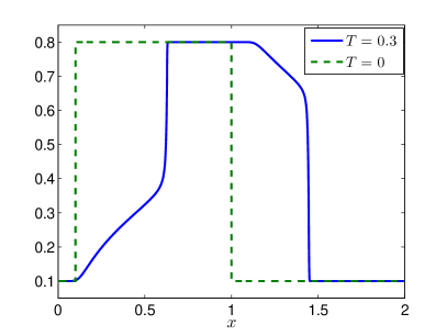
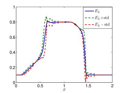
Figure 1. Left: One sample of the random entropy solution of (5.1) with (5.4), (5.2) and (5.3) at time $T=0.3$ computed on a mesh with $4096$ points. Right: A sample of the estimator $E^{L}[s(\cdot,t)]$ for (5.1) with (5.4), (5.2) and (5.3) at time $T=0.3$ (solid line), the dashed lines denote $E^{L}[s(\cdot,t)]$ $\pm$ standard deviation.

We will use this sample of the MLMC estimator as a reference solution when estimating the approximation errors and computing the convergence rates.

In order to compute an estimate on the error of the approximation of the mean by the MLMC estimator $E^{L}[s(t)]$ in the $L^{2}(\Omega;L^{1}(\mathbb{R}))$-norm, we use the relative error estimator introduced in [29] based on a Monte Carlo quadrature in the stochastic domain: By $U_{\mathrm{ref}}$ we denote a reference solution and $\{U_{k}\}_{k=1,\dots,N}$ a sequence of independent approximate solutions $E^{L}[s(t)]$ obtained by running the MLMC-FDM solver $N$ times, corresponding to $N$ realizations in the stochastic domain. Then we estimate the relative error by

(5.5) $$\mathcal{R}E=\sqrt{\sum_{k=1}^{N}(\mathcal{R}E_{k})^{2}/N},$$

where

$$\mathcal{R}E_{k}=100\times\frac{\|U_{\mathrm{ref}}-U_{k}\|_{\ell^{1}}}{\|U_{\mathrm{ref}}\|_{\ell^{1}}}\;.$$

In [29], the sensitivity of the error with respect to the parameter $N$ is investigated. In the present numerical experiments, we use $N=5$ which was shown to be sufficient for most problems [29, 30]. In Table 1 the errors (5.5) versus the resolution $\Delta x_{L}$ at the finest level $L$ of the MLMC estimator and versus the average time (in seconds) needed to compute one sample of the MLMC estimator are shown ($L=0,\dots,5$). We observe that the calculated convergence rates are $\approx 0.66$ (explicit scheme) and $\approx 0.75$ (implicit scheme) with respect to the resolution and $\approx 0.32$ (explicit scheme) and $0.38$ (implicit scheme) with respect to work. This is better than what we would expect from the theory, cf. (4.28) and (4.30a), (4.30b). However, they decrease as we refine the mesh, which might indicate that we are not in the asymptotic regime yet.

$L$	$\mathcal{R}E$	${\Delta x}_{L}$	run time	$\left|E^{L}(s(t))\right|_{BV([0,2])}$	$\|E^{L}(s(t))\|_{L^{\infty}([0,2])}$
$0$	16.54	$2^{-3}$	0.45	1.37	0.79
$1$	10.25	$2^{-4}$	2.48	1.4	0.8
$2$	6.13	$2^{-5}$	10.31	1.42	0.81
$3$	3.53	$2^{-6}$	40.58	1.44	0.81
$4$	2.06	$2^{-7}$	159.6	1.48	0.81
$5$	1.68	$2^{-8}$	632.37	1.58	0.82
average rate		0.66	-0.32

Table 1. Relative mean square errors (as defined in (5.5)) versus grid size at highest level and time (in seconds), for problem (5.1) with (5.4), (5.2) and (5.3), for the MLMC solver with the explicit difference scheme.

$L$	$\mathcal{R}E$	${\Delta x}_{L}$	run time	$\left|E^{L}(s(t))\right|_{BV([0,2])}$	$\|E^{L}(s(t))\|_{L^{\infty}([0,2])}$
$0$	22.89	$2^{-3}$	0.65	1.3	0.76
$1$	14.69	$2^{-4}$	3.53	1.39	0.8
$2$	9.27	$2^{-5}$	13.29	1.43	0.81
$3$	5.57	$2^{-6}$	47.7	1.44	0.81
$4$	3.15	$2^{-7}$	174.8	1.47	0.81
$5$	1.68	$2^{-8}$	659.7	1.5	0.81
average rate		0.75	-0.38

Table 2. Relative mean square errors (as defined in (5.5)) versus grid size at highest level and CPU time (in seconds), for problem (5.1) with (5.4), (5.2) and (5.3), for the MLMC solver with time-stepping by the implicit difference scheme.

In the last two columns of Tables 1, 2 the average total variation and $L^{\infty}$-norm of $E^{L}(s(t))$ at the different refinement levels are given. We observe that they slightly increase, but not as much as the bounds

$$\left|E^{L}(s(t))\right|_{BV(\mathbb{R})} =\biggl{|}\sum_{\ell=0}^{L}\frac{1}{M_{\ell}}\sum_{i=0}^{M_{\ell}}(s_{\ell}^{i}-s_{\ell-1}^{i})\biggr{|}_{BV(\mathbb{R})}\leq\sum_{\ell=0}^{L}\frac{1}{M_{\ell}}\sum_{i=0}^{M_{\ell}}\left|s_{\ell}^{i}-s_{\ell-1}^{i}\right|_{BV(\mathbb{R})}$$

$$\leq 2(L+1)\,\left|s_{0}\right|_{BV(\mathbb{R})}$$

$$\left\|E^{L}(s(t))\right\|_{L^{\infty}(\mathbb{R})} =\biggl{\|}\sum_{\ell=0}^{L}\frac{1}{M_{\ell}}\sum_{i=0}^{M_{\ell}}(s_{\ell}^{i}-s_{\ell-1}^{i})\biggr{\|}_{L^{\infty}(\mathbb{R})}\leq\sum_{\ell=0}^{L}\frac{1}{M_{\ell}}\sum_{i=0}^{M_{\ell}}\left\|s_{\ell}^{i}-s_{\ell-1}^{i}\right\|_{L^{\infty}(\mathbb{R})}$$

$$\leq 2(L+1)\,\left\|s_{0}\right\|_{L^{\infty}(\mathbb{R})},$$

would imply.

5.2. Random residual saturation

In the following numerical example, we will model the relative permeabilities by the random variables

(5.6) $$\lambda^{w}(s)=\mathbf{1}_{s>s_{w}^{*}(\omega_{1})}(s)\frac{\left(s-s_{w}^{*}(\omega_{1})\right)^{2}}{\left(1-s_{w}^{*}(\omega_{1})\right)^{2}},\quad\lambda^{o}(s)=\mathbf{1}_{s\leq s_{o}^{*}(\omega_{2})}(s)\left(1-\frac{s}{s_{o}^{*}(\omega_{2})}\right)^{2},$$

$$\text{with}\quad s^{*}_{w}(\omega_{1})\sim\mathcal{U}(0.05,0.35),\quad s^{*}_{o}(\omega_{2})\sim\mathcal{U}(0.6,0.95),\quad s^{*}_{w}(\omega_{1})\perp s^{*}_{o}(\omega_{2}),$$

that is we assume that the residual saturations $s^{*}_{w}$, $s^{*}_{o}$ are independent, uniformly distributed random variables. As initial data, we use again use (5.4) with periodic boundary conditions.

The resulting $(s_{0},f,A)(\omega_{1},\omega_{2};\cdot)$ again satisfies assumptions (3.11) – (3.17), so that the random entropy solution from Definition 3.4 exists and Theorems 3.5, 4.9 apply. In Figure 2 on the left hand side, we have plotted a sample $s(\omega;t,\cdot)$ of the random entropy solution at time $T=0.3$ and on the right hand side we have plotted a sample of the MLMC-FDM estimator $E^{L}(s(t))$ for $M_{0}=8$, $L=8$, $\Delta x_{0}=2^{-3}$, $K=1$ and CFL-number $0.4$. We observe that the variance is larger compared to the variance in the previous example.

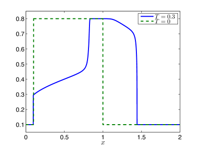
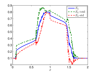
Figure 2. Left: One sample of the random entropy solution of (5.1) with (5.4), (5.2) and (5.6) at time $T=0.3$ computed on a mesh with $4096$ points. Right: A sample of the estimator $E^{L}[s(\cdot,t)]$ for (5.1) with (5.4), (5.2) and (5.6) at time $T=0.3$ (solid line), the dashed lines denote $E^{L}[s(\cdot,t)]$ $\pm$ standard deviation.

We will use this sample of the MLMC estimator as a reference solution when estimating the approximation errors and computing the convergence rates. Moreover, we will again compute an estimate of the $L^{2}(\Omega;L^{1}(\mathbb{R}))$-error using the error estimator defined in (5.5) with $N=5$.

In Tables 3, 4 the errors (5.5) versus the resolution $\Delta x_{L}$ at the finest level $L$ of the MLMC estimator and versus the average time (in seconds) needed to compute one sample of the MLMC estimator are shown ($L=0,\dots,5$). We observe that the approximate convergence rates are $\approx 0.43$ (explicit scheme) and $\approx 0.57$ (implicit scheme) with respect to the resolution and $\approx 0.21$ (explicit scheme) and $\approx 0.37$ (implicit scheme) with respect to work, which is again better than what we would expect from the theory, cf. (4.28) and (4.30a), (4.30b). However, it decreases as we refine the mesh, which might indicate that we are not in the asymptotic regime yet. We also note that the rates are lower than in the previous example.

$L$	$\mathcal{R}E$	${\Delta x}_{L}$	run time	$\left|E^{L}(s(t))\right|_{BV([0,2])}$	$\|E^{L}(s(t))\|_{L^{\infty}([0,2])}$
$0$	12.36	$2^{-3}$	0.48	1.31	0.76
$1$	8.67	$2^{-4}$	2.69	1.38	0.78
$2$	5.44	$2^{-5}$	10.82	1.47	0.82
$3$	4.33	$2^{-6}$	41.97	1.63	0.83
$4$	3.32	$2^{-7}$	164.53	1.73	0.82
$5$	2.77	$2^{-8}$	679.27	2.04	0.82
average rate		0.43	-0.21

Table 3. Relative mean square errors (as defined in (5.5)) versus grid size at highest level and time (in seconds), for problem (5.1) with (5.4), (5.2) and (5.6) (explicit scheme in MLMC solver).

$L$	$\mathcal{R}E$	${\Delta x}_{L}$	run time	$\left|E^{L}(s(t))\right|_{BV([0,2])}$	$\|E^{L}(s(t))\|_{L^{\infty}([0,2])}$
$0$	16.0	$2^{-3}$	1.16	1.23	0.72
$1$	9.34	$2^{-4}$	3.9	1.37	0.78
$2$	5.54	$2^{-5}$	11.52	1.44	0.8
$3$	4.54	$2^{-6}$	31.29	1.61	0.82
$4$	2.61	$2^{-7}$	88.8	1.71	0.81
$5$	2.29	$2^{-8}$	265.46	2.05	0.81
average rate		0.57	-0.37

Table 4. Relative mean square errors (as defined in (5.5)) versus grid size at highest level and time (in seconds), for problem (5.1) with (5.4), (5.2) and (5.6) (implicit scheme in MLMC solver).

5.3. Sine wave initial data

As a third example, we have tested the convergence rates on Problem (5.1), (5.2), (5.3) with sine wave initial data,

(5.7) $$s_{0}(x)=\sin(4\pi x),\quad x\in[0,0.5],$$

In Figure 3, on the left hand side, we have plotted a sample of the solution computed on a mesh with $2048$ points at time $T=0.5$ and on the right hand side a sample of the MLMC estimator for $L=7$, ${\Delta x}_{0}=1/16$, $M_{0}=8$ and CFL-number $0.4$, also at time $T=0.5$. We observe that the approximation looks quite smooth and that the variance is evenly distributed over the whole spatial domain in contrast to the previous examples.

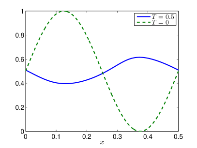
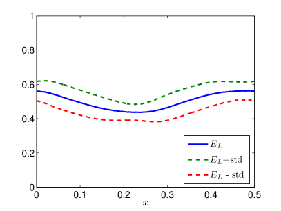
Figure 3. Left: One sample of the random entropy solution of (5.1) with (5.7), (5.2) and (5.3) at time $T=0.5$ computed on a mesh with $2048$ points. Right: A sample of the estimator $E^{L}[s(\cdot,t)]$ for (5.1) with (5.7), (5.2) and (5.3) at time $T=0.5$ (solid line), the dashed lines denote $E^{L}[s(\cdot,t)]$ $\pm$ standard deviation.

In Tables 5, 6 the estimates (5.5) on the $L^{2}(\Omega;L^{1}(\mathbb{R}))$-error for $N=5$ are displayed and compared to the mesh resolution at the finest level and the run time.

$L$	$\mathcal{R}E$	${\Delta x}_{L}$	run time	$\left|E^{L}(s(t))\right|_{BV([0,2])}$	$\|E^{L}(s(t))\|_{L^{\infty}([0,2])}$
$0$	8.11	$2^{-4}$	1.68	0.008	0.5
$1$	6.71	$2^{-5}$	9.94	0.055	0.51
$2$	5.26	$2^{-6}$	43.36	0.131	0.53
$3$	3.35	$2^{-7}$	179.02	0.18	0.54
$4$	1.85	$2^{-8}$	721.99	0.253	0.56
Average Rate		0.53	-0.25

Table 5. Relative mean square errors (as defined in (5.5)) versus grid size at highest level and time, for problem (5.1) with (5.7), (5.2) and (5.3) (explicit deterministic solver in MLMC method).

$L$	$\mathcal{R}E$	${\Delta x}_{L}$	run time	$\left|E^{L}(s(t))\right|_{BV([0,2])}$	$\|E^{L}(s(t))\|_{L^{\infty}([0,2])}$
$0$	19.23	$2^{-3}$	0.7	0.27	0.58
$1$	5.71	$2^{-4}$	3.94	0.13	0.54
$2$	9.78	$2^{-5}$	16.33	0.08	0.52
$3$	6.6	$2^{-6}$	62.58	0.08	0.52
$4$	4.91	$2^{-7}$	235.8	0.14	0.53
$5$	3.52	$2^{-8}$	898.15	0.22	0.55
Average Rate		0.39	-0.19

Table 6. Relative mean square errors (as defined in (5.5)) versus grid size at highest level and time, for problem (5.1) with (5.7), (5.2) and (5.3) (implicit solver in MLMC method).

We find a convergence rate of $\approx 0.53$ (explicit scheme) and $\approx 0.39$ (implicit scheme) versus resolution and $\approx 0.25$ (explicit scheme) and $\approx 0.19$ (implicit scheme) versus run time. We also observe that the rates improve when the mesh is refined. Interestingly, for this example the convergence rates for the MLMC solver with the implicit scheme are worse than those for the explicit scheme in contrast to the previous examples. The reason could be the samples of the implicit scheme at level $L=1$ which are closer to the reference solution than the following ones at higher levels. This decreases the average rate for the implicit scheme.

References

- [1] M. Afif and B. Amaziane. Convergence of finite volume schemes for a degenerate convection-diffusion equation arising in flow in porous media. Comput. Methods Appl. Mech. Engrg., 191(46):5265–5286, 2002.
- [2] F. Bouchut, F. R. Guarguaglini, and R. Natalini. Diffusive bgk approximations for nonlinear multidimensional parabolic equations. Indiana Univ. Math. J., 49(2):723–749, 2000.
- [3] J. Boussinesq. Recherches théoriques sur l′écoulement des nappes d′eau infiltrées dans le sol et sur le débit des sources. Journal de mathématiques pures et appliquées, 10:5–78, 1904.
- [4] J. Carrillo. Entropy solutions for nonlinear degenerate problems. Arch. Ration. Mech. Anal., 147(4):269–361, 1999.
- [5] G.-Q. Chen and B. Perthame. Well-posedness for non-isotropic degenerate parabolic-hyperbolic equations. Ann. Inst. H. Poincaré Anal. Non Linéaire, 20(4):645–668, 2003.
- [6] B. Cockburn and G. Gripenberg. Continuous dependence on the nonlinearities of solutions of degenerate parabolic equations. Journal of differential equations, 151(2):231–251, 1999.
- [7] B. Cockburn and C.-W. Shu. The local discontinuous Galerkin method for time-dependent convection-diffusion systems. SIAM J. Numer. Anal., 35(6):2440–2463, 1998.
- [8] G. Da Prato and J. Zabczyk. Stochastic equations in infinite dimensions, volume 44 of Encyclopedia of Mathematics and its Applications. Cambridge University Press, Cambridge, 1992.
- [9] C. M. Dafermos. Hyperbolic conservation laws in continuum physics, volume 325 of Grundlehren der Mathematischen Wissenschaften [Fundamental Principles of Mathematical Sciences]. Springer-Verlag, Berlin, third edition, 2010.
- [10] S. Evje and K. H. Karlsen. Degenerate convection-diffusion equations and implicit monotone difference schemes. In Hyperbolic problems: theory, numerics, applications, Vol. I (Zürich, 1998), volume 129 of Internat. Ser. Numer. Math., pages 285–294. Birkhäuser, Basel, 1999.
- [11] S. Evje and K. H. Karlsen. Viscous splitting approximation of mixed hyperbolic-parabolic convection-diffusion equations. Numerische Mathematik, 83(1):107–137, 1999.
- [12] S. Evje and K. H. Karlsen. Monotone difference approximations of BV solutions to degenerate convection-diffusion equations. SIAM J. Numer. Anal., 37(6):1838–1860, 2000.
- [13] S. Evje and K. H. Karlsen. An error estimate for viscous approximate solutions of degenerate parabolic equations. J. Nonlinear Math. Phys., 9(3):262–281, 2002.
- [14] S. Evje, K. H. Karlsen, and N. H. Risebro. A Continuous Dependence Result For Nonlinear Degenerate Parabolic Equations With Spatially Dependent Flux Function. In Proc. Hyp, pages 337–346, 2000.
- [15] R. Eymard, T. Gallouët, and R. Herbin. Convergence of a finite volume scheme for nonlinear degenerate parabolic equations. Numerische Mathematik, 92:41–82, 2002.
- [16] R. Eymard, T. Gallouët, and R. Herbin. Error estimate for approximate solutions of a nonlinear convection-diffusion problem. Advances in Differential Equations, 7(4):419–440, 2002.
- [17] E. Godlewski and P.-A. Raviart. Hyperbolic systems of conservation laws, volume 3/4 of Mathématiques & Applications (Paris) [Mathematics and Applications]. Ellipses, Paris, 1991.
- [18] R. Helmig, A. Weiss, and B. Wohlmuth. Dynamic capillary effects in heterogeneous porous media. Computational Geosciences, 11(3):261–274, 2007.
- [19] H. Holden, K. H. Karlsen, and K.-A. Lie. Operator splitting methods for degenerate convection-diffusion equations. I. Convergence and entropy estimates. In Stochastic processes, physics and geometry: new interplays, II (Leipzig, 1999), volume 29 of CMS Conf. Proc., pages 293–316. Amer. Math. Soc., Providence, RI, 2000.
- [20] H. Holden, K. H. Karlsen, and N. H. Risebro. On uniqueness and existence of entropy solutions of weakly coupled systems of nonlinear degenerate parabolic equations. Electron. J. Differential Equations, pages No. 46, 31, 2003.
- [21] K. H. Karlsen, N. H. Risebro, and E. B. Storrøsten. error estimates for difference approximations of degenerate convection-diffusion equations. Preprint, to appear in Math. Comp.
- [22] K. H. Karlsen, N. H. Risebro, and E. B. Storrøsten. error estimates for difference approximations of degenerate convection-diffusion equations in multi-dimensions. Preprint, http://www.mn.uio.no/math/personer/vit/erlenbs/convergenceratemultid.pdf.
- [23] K. H. Karlsen, N. H. Risebro, and J. D. Towers. On a nonlinear degenerate parabolic transport-diffusion equation with a discontinuous coefficient. Electron. J. Differential Equations, pages No. 93, 23, 2002.
- [24] K. H. Karlsen, N. H. Risebro, and J. D. Towers. Upwind difference approximations for degenerate parabolic convection-diffusion equations with a discontinuous coefficient. IMA J. Numer. Anal., 22(4):623–664, 2002.
- [25] S. N. Kružkov. First order quasilinear equations with several independent variables. Mat. Sb. (N.S.), 81 (123):228–255, 1970.
- [26] A. Kurganov and E. Tadmor. New high-resolution central schemes for nonlinear conservation laws and convection-diffusion equations. J. Comput. Phys., 160(1):241–282, 2000.
- [27] L. Leibenzon. Complete Works, volume 2, chapter The Motion of a Gas in a Porous Medium. Acad. Sciences URSS, Moscow, 1930.
- [28] S. Mishra, N. H. Risebro, C. Schwab, and S. Tokareva. Numerical solution of scalar conservation laws with random flux functions. Technical Report 2012-35, Seminar for Applied Mathematics, ETH Zürich, Switzerland, 2012.
- [29] S. Mishra and C. Schwab. Sparse tensor multi-level Monte Carlo finite volume methods for hyperbolic conservation laws with random initial data. Math. Comp., 81(280):1979–2018, 2012.
- [30] S. Mishra, C. Schwab, and J. Sukys. Monte Carlo and multi-level Monte Carlo finite volume methods for uncertainty quantification in nonlinear systems of balance laws. 2012.
- [31] S. Mishra, C. Schwab, and J. Šukys. Multi-level Monte Carlo finite volume methods for uncertainty quantification in nonlinear systems of balance laws. Von Karman Institute Lecture Notes UQLNCSE6 (to appear), 2013.
- [32] M. Muskat and M. W. Meres. The flow of heterogeneous fluids through porous media. Physics, 7(9):346–363, 1936.
- [33] M. Ohlberger. A posteriori error estimates for vertex centered finite volume approximations of convection-diffusion-reaction equations. M2AN Math. Model. Numer. Anal., 35(2):355–387, 2001.
- [34] O. A. Oleĭnik and S. N. Kružkov. Quasi-linear parabolic second-order equations with several independent variables. Uspehi Mat. Nauk, 16(5 (101)):115–155, 1961.
- [35] J. Smoller. Shock waves and reaction-diffusion equations, volume 258 of Grundlehren der Mathematischen Wissenschaften [Fundamental Principles of Mathematical Sciences]. Springer-Verlag, New York, second edition, 1994.
- [36] A. I. Volpert. Generalized solutions of degenerate second-order quasilinear parabolic and elliptic equations. Adv. Differential Equations, 5(10-12):1493–1518, 2000.
- [37] A. I. Volpert and S. I. Hudjaev. The Cauchy problem for second order quasilinear degenerate parabolic equations. Mat. Sb. (N.S.), 78 (120):374–396, 1969.
- [38] Y. B. Zel′dovich and Y. P. Raizer. Physics of Shock Waves and High-Temperature Hydrodynamic Phenomena, volume 2. Academic Press, New York, 1966.