GooFit: A library for massively parallelising maximum-likelihood fits

Abstract

Fitting complicated models to large datasets is a bottleneck of many analyses. We present GooFit, a library and tool for constructing arbitrarily-complex probability density functions (PDFs) to be evaluated on nVidia GPUs or on multicore CPUs using OpenMP. The massive parallelisation of dividing up event calculations between hundreds of processors can achieve speedups of factors 200-300 in real-world problems.

1 Introduction

Parameter estimation is a crucial part of many physics analyses. GooFit is an interface between the MINUIT minimisation algorithm and a parallel processor - either a Graphics Processing Unit (GPU) or a multicore CPU - which allows a probability density function (PDF) to be evaluated in parallel. Since PDF evaluation on large datasets is usually the bottleneck in the MINUIT algorithm, this can result in speedups of up to $\sim 300$ in real problems - which can be the difference between waiting overnight for the answer, or making a cup of tea.

GooFit is named in homage to the fitting package RooFit [5], with the G standing for GPU. The overall flow of a program using GooFit - create variables, create PDF objects, load data, fit, as shown in listing 1 - should be somewhat familiar to RooFit users.

2 GooFit code

The original intention of GooFit was to give users access to the parallelising power of CUDA [2], nVidia’s programming language for GPUs, without requiring them to write CUDA code. By abstracting the thread-management code using the Thrust library [1], we have extended the possible parallel platforms; currently GooFit supports CUDA and OpenMP. In the future we hope also to include Thrust’s TBB backend, as well as any other backends that the Thrust developers add.

At the most basic level, GooFit objects representing PDFs, GooPdfs, can be created and combined in plain C++. Only if a user needs to represent a function outside the existing GooFit classes does she need to do any CUDA coding; Section 4 shows how to create new PDF classes. We intend, however, that this should be a rarity, and that the existing PDF classes should cover the most common cases.

A GooFit program has four main components:

• The PDF that models the physical process, represented by a GooPdf object.

• The fit parameters with respect to which the likelihood is maximised, represented by Variables contained in the GooPdf.

• The data, gathered into a DataSet object containing one or more Variables.

• A FitManager object which forms the interface between Minuit (or, in principle, any maximising algorithm) and the GooPdf.

Listing 1 shows a simple fit of an exponential function.

Listing 1.

Fit for unknown parameter $\alpha$ in $e^{\alpha x}$. GooFit classes are shown in red, important operations in blue.

int main (int argc, char** argv) {

  // Independent variable (name, lower limit, upper limit)

  Variable* xvar = new Variable("xvar", 0, log(1+RAND_MAX/2));

  // Create data set

  UnbinnedDataSet data(xvar);

  for (int i = 0; i < 100000; ++i) {

    // Generate toy event

    xvar->value = xvar->upperlimit - log(1+rand()/2);

    // ...and add to data set.

    data.addEvent();

  }

  // Create fit parameter (name, initial value, step size, lower and upper limit)

  Variable* alpha = new Variable("alpha", -2, 0.1, -10, 10);

  // Create GooPdf object - name, independent variable, fit parameter.

  ExpPdf* exppdf = new ExpPdf("exppdf", xvar, alpha);

  // Move data to GPU

  exppdf->setData(&data);

  FitManager fitter(exppdf);

  fitter.fit();

  return 0;

}

The example code contains two different uses of the Variable class: xvar represents the measured (in this toy example, randomly generated) experimental results, while alpha represents the model parameter to be determined - in this case a decay constant. In the latter case we supply an initial value for the fit to start with and a guess at a reasonable step size, in addition to upper and lower allowed limits. For data points, which will not vary in the fit, the initial value and step size are not needed, so we use a Variable constructor which does not require them.

The UnbinnedDataSet class is supplied, at construction time, with pointers to the Variables it is to contain - in general by means of a vector of Variable*, but for convenience in the single-observable case there is a constructor that takes a single pointer. It is then filled by means of the addEvent method, which creates a “row” or “event” within the dataset, containing the values, at the time of the setData call, of the comprising Variables. An example may be helpful to visualising this:

  Variable* xvar = new Variable("xvar", 0, log(1+RAND_MAX/2));

  UnbinnedDataSet data(xvar);  // Data set is empty

  xvar->value = 3;  // Still empty

  data.addEvent();  // Now contains one event, value 3

  xvar->value = 5;

  data.addEvent();  // Two events: 3, 5

  xvar->value = 1;

  data.addEvent();  // Three events: 3, 5, 1Note that UnbinnedDataSet stores its events in host memory, that is, not on the GPU; not until the setData method of a GooPdf is called are the events moved to the GPU or other target device.

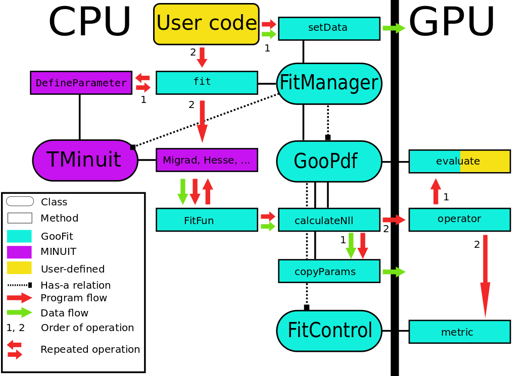
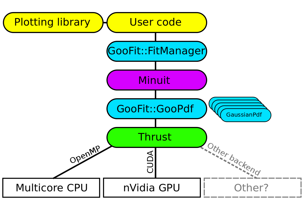
Figure 1: Control and data flow of a GooFit program (left) and overall architecture of GooFit (right).

The fit method of the FitManager class does two things: First, it sets up the Minuit [4, 3] fit by calling the DefineParameter method on each Variable representing a fit parameter. Second, it passes control to MINUIT’s mnmigr method, which will in turn call GooFit’s evaluation method for different sets of parameters until it converges or gives up. The program flow is illustrated in Figure 1. Notice, on the device side, the separate calls to the evaluate method under GooPdf, and the metric method under FitManager; this allows switching between, for example, maximum-likelihood and chi-squared fits without changing any PDF creation code.

Calls to the device-side methods are done by the Thrust template library; this allows us to switch the execution backend by means of a compile-time switch. In particular, GooFit currently supports CUDA and OpenMP parallelisation. Figure 1 shows the overall organisation of GooFit, with user code at the top and Thrust talking to the parallelising target at the bottom. Note that Minuit, in the middle, can in principle be replaced by any algorithm for searching through parameter space.

3 Combining functions

To create arbitrarily complex PDFs, the user can combine simple ones like the exponential and Gaussian in several ways, the most common being addition and multiplication. For example, a two-dimensional distribution, described by a separate exponential in each of two variables $x$ and $y$, may be represented as a ProdPdf object, as shown in Listing 2.

Listing 2.

Product of two exponentials.

int main (int argc, char** argv) {

  Variable* xvar = new Variable("xvar", 0, log(1+RAND_MAX/2));

  Variable* yvar = new Variable("yvar", 0, log(1+RAND_MAX/2));

  vector<Variable*> varList;

  varList.push_back(xvar);

  varList.push_back(yvar);

  UnbinnedDataSet data(varList);

  for (int i = 0; i < 100000; ++i) {

    xvar->value = xvar->upperlimit - log(1+rand()/2);

    yvar->value = yvar->upperlimit - log(1+rand()/2);

    data.addEvent();

  }

  Variable* alpha_x = new Variable("alpha_x", -2.4, 0.1, -10, 10);

  Variable* alpha_y = new Variable("alpha_y", -1.1, 0.1, -10, 10);

  vector<PdfBase*> pdfList;

  pdfList.push_back(new ExpPdf("exp_x", xvar, alpha_x));

  pdfList.push_back(new ExpPdf("exp_y", yvar, alpha_y));

  ProdPdf* product = new ProdPdf("product", pdfList);

  product->setData(&data);

  FitManager fitter(product);

  fitter.fit();

  return 0;

}

In addition to products, GooFit implements sums of PDF through the AddPdf class, convolutions by means of the ConvolutionPdf, and function composition, ie $f(g(x))$, in the CompositePdf class. Finally, the MappedPdf allows the construction of functions with different form depending on a set parameter, that is

$$F(x) = \left\{\begin{array}[]{rl}A(x)&\mbox{ if $x\in[x_{0},x_{1})$}\\ B(x)&\mbox{ if $x\in[x_{1},x_{2})$}\\ \ldots&\\ Z(x)&\mbox{ if $x\in[x_{N-1},x_{N}]$}\end{array}\right.$$

All these combined PDF classes can be nested arbitrarily deeply.

4 Adding new PDFs

For advanced users who need additional PDFs, GooFit makes it easy to write a new PDF class. There are two steps to the process:

• Write an evaluation method with the required signature, using the provided index array to look up parameters and observables. An example is shown in Listing 3.

• Create a C++ class inheriting from GooPdf, in which the constructor populates the index array through the registerParameter method. Listing 4 shows an example.

That’s it! Putting the new FooPdf.cu and FooPdf.hh files in the PDFs directory of GooFit will cause them to be compiled with the rest of the framework, and be available for use in the same way as the pre-existing PDFs.

Listing 3.

Evaluation function for a Gaussian PDF. Note the double indirection of the index-array lookups. Here fptype indicates a floating-point number, by default double precision.

__device__ fptype device_Gaussian (fptype* evt, fptype* p, unsigned int* indices) {

  fptype x = evt[indices[2 + indices[0]]];

  fptype mean = p[indices[1]];

  fptype sigma = p[indices[2]];

  fptype ret = EXP(-0.5*(x-mean)*(x-mean)/(sigma*sigma));

  return ret;

}

__device__ device_function_ptr ptr_to_Gaussian = device_Gaussian;

Listing 4.

Populating the index array used in Listing 3.

__host__ GaussianPdf::GaussianPdf (std::string n, Variable* _x,

                                   Variable* mean, Variable* sigma)

  : GooPdf(_x, n)

{

  std::vector<unsigned int> pindices;

  pindices.push_back(registerParameter(mean));

  pindices.push_back(registerParameter(sigma));

  cudaMemcpyFromSymbol((void**) &host_fcn_ptr, ptr_to_Gaussian, sizeof(void*));

  initialise(pindices);

}

5 Results

To ensure the usefulness of GooFit in real-world physics problems we have, simultaneously with developing GooFit, used it as our fitting tool in a time-dependent Dalitz-plot analysis of the decay $D^{0}\to\pi^{+}\pi^{-}\pi^{0}$. This fit has been our “driver” for GooFit, in that every time we needed a feature for the physics, we added it to the GooFit engine. This mixing fit is rather complex, involving, for the signal component, 16 amplitudes (each a complex number) to describe the Dalitz-plot distribution, a time component where hyperbolic and trigonometric functions are convolved with Gaussian resolution functions, and a distribution of the uncertainty $\sigma_{t}$ on the decay time which varies across the Dalitz plot. All in all, there are about 40 free parameters in the fit, and the data set is roughly a hundred thousand events; running this on one core of a modern CPU takes about five hours, depending on the data. Using GooFit with a CUDA backend, this is reduced to a much more comfortable one minute, a speedup factor in the region of 300, relative to the original hand-coded CPU implementation. Testing with the OpenMP backend, as shown in Table 2, indicates that some part of this speedup is due to the reorganising of the code, or perhaps of the memory, whose management differs between the original CPU implementation and GooFit.

In addition to the mixing fit described above, we have tested GooFit on “Zach’s fit”, named for a (now graduated) student of our group. This is a binned fit, extracting the $D^{*+}$ line width from measurements of the $D^{*+}-D$ mass difference, and involving an underlying relativistic P-wave Breit-Wigner convolved with a resolution function comprising several Gaussians. In its original RooFit implementation this fit takes about 7 minutes on our workstation ‘Cerberus’. With GooFit this is reduced down to a few seconds; however, the speedup is not as impressive as with the mixing fit. We do not fully understand the differences, but believe it is partly because a binned fit, with only a few thousand PDF evaluations per MINUIT iteration, does not take as much advantage of the massive parallelisation of the GPU as does an unbinned fit with a hundred thousand events.

As shown in Table 1, we have measured GooFit’s performance on three different platforms: Our workstation Cerberus, the ‘Oakley’ computer farm of the Ohio Supercomputer Center, and the laptop ‘Starscream’ with a mid-range 650M GPU. In addition we have tested earlier versions of GooFit on K10 and K20 boards, with speedups of about a factor 2 relative to the C2050.

The execution times shown in Table 2 are for Minuit fits using the Migrad algorithm; time to load data into memory and create PDF objects is not shown, on the assumption that these are negligible for realistic problems. It is worth noting that in going from the original implementations of the two fits (run on one core of Cerberus) to the GooFit implementation with one OpenMP thread, there is already a speedup in the range of 6-7. We believe that this is due to differences in memory layout - GooFit represents its events as a single large array of floating-point numbers - and, in the case of the Zach fit, perhaps also to the large number of virtual-function calls in inner loops of the RooFit implementation.

As we increase the number of OpenMP threads, we see a nearly-linear speedup, ie times inversely proportional to the number of threads, up until the number of threads equals the number of cores. After this there is no gain from adding more threads, except for the sweet spot of having exactly twice as many threads as there are physical cores - this takes full advantage of the hyperthreading capacity of these processors, and gives a 30% speedup on Cerberus and a 50% speedup on the more recent Starscream. It is clear that the power of a GPU to speed up fits varies with the precise problem, but in the best case a C2050 GPU can be 5 times as fast as the same code parallelised using OpenMP and taking full advantage of a powerful dual quad-core CPU.

Name	Chip	Cores	Clock [GHz]	RAM [Gb]	OS
Cerberus (CPU)	Intel Xeon E5520	8*	2.27	24	Fedora 14
Cerberus (GPU)	nVidia C2050	448	1.15	3	Fedora 14
Starscream (CPU)	Intel i7-3610QM	4*	2.3	8	Ubuntu 12.04
Starscream (GPU)	nVidia 650M	384	0.9	1	Ubuntu 12.04
Oakley	nVidia C2070	448	1.15	6	RedHat 6.3

Table 1: Some specifications of the testing platforms. Asterisks next to the number of cores indicate hyperthreading - two virtual processors per physical core.

	Mixing fit		Zach’s fit
Platform	Time [s]	Speedup	Time [s]	Speedup
Original CPU	19489	1.0	438	1.0
Cerberus OMP (1)	3056	6.4	60.6	7.2
Cerberus OMP (2)	1563	12.5	31.0	14.1
Cerberus OMP (4)	809	24.1	18.2	24.1
Cerberus OMP (8)	432	45.1	9.2	47.6
Cerberus OMP (12)	534	36.5	12.2	35.9
Cerberus OMP (16)	326	59.8	6.9	63.5
Cerberus OMP (24)	432	45.1	9.5	46.1
Cerberus C2050	64	304.5	5.8	75.5
Starscream OMP (1)	2042	9.5	37.1	11.8
Starscream OMP (2)	1056	18.5	19.2	22.8
Starscream OMP (4)	562	34.6	10.8	40.6
Starscream OMP (8)	407	47.9	6.9	63.5
Starscream 650M	212	91.9	18.6	23.5
Oakley C2070	54	360.1	5.4	81.1

Table 2: Timing results and speedups for the test fits.

6 Summary

We have developed GooFit for use in real-world physics problems, and have achieved speedups of $\sim 300$ in particular analyses. We have created a robust framework that is easy enough for a new graduate student to use, but flexible enough that the most advanced analyses will find it useful.

GooFit’s source code lives in a GitHub repository at https://github.com/GooFit, which also includes a manual and several example fits to get the new user started.

Development of GooFit is supported by NSF grant NSF-1005530. We are grateful for valuable suggestions and help from Cristoph Deil and feedback and user reports from Olli Lupton and Stefanie Reichert. Jan Veverka and Helge Voss contributed implementations of the bifurcated Gaussian and Landau distributions. The Ohio Supercomputer Center made their computer farm “Oakley” available for development, for testing, and for GooFit outreach workshops. nVidia’s Early Access Program made it possible to test our code on K10 and K20 boards.

References

References

- [1] N. Bell and J. Hoberock. Thrust: A Productivity-Oriented Library for CUDA. GPU Computing Gems: Jade Edition, 2012.
- [2] NVIDIA Corp. NVIDIA CUDA C Programming Best Practices Guide - CUDA toolkit 2.3, 2009.
- [3] W. C. Davidon. Variable metric method for minimization. SIAM Journal on Optimization, 1(1), 1991.
- [4] F. James. Minuit - function minimization and error analysis. CERN Program Library Long Writeup, D506, 1972.
- [5] W. Verkerke and D.P. Kirkby. The RooFit toolkit for data modeling. eConf, C0303241:MOLT007, 2003.