Factorization of exclusive electroinduced two-nucleon knockout

Abstract

We investigate the factorization properties of the exclusive electroinduced two-nucleon knockout reaction $A(e,e^{\prime}pN)$. A factorized expression for the cross section is derived and the conditions for factorization are studied. The $A(e,e^{\prime}pN)$ cross section is shown to be proportional to the conditional center-of-mass (c.m.) momentum distribution for close-proximity pairs in a state with zero relative orbital momentum and zero radial quantum number. The width of this conditional c.m. momentum distribution is larger than the one corresponding with the full c.m. momentum distribution. It is shown that the final-state interactions (FSIs) only moderately affect the shape of the factorization function for the $A(e,e^{\prime}pN)$ cross sections. Another prediction of the proposed factorization is that the mass dependence of the $A(e,e^{\prime}pp)$ $[A(e,e^{\prime}pn)]$ cross sections is much softer than $\frac{Z(Z-1)}{2}$ $[NZ]$.

I Introduction

In recent years, substantial progress has been made in exploring the dynamics of short-range correlations (SRCs) in nuclei. On the experimental side, exclusive $A(p,2p+n)$ Tang et al. (2003) and $A(e,e^{\prime}pN)$ Niyazov et al. (2004); Shneor et al. (2007); Subedi et al. (2008) measurements have probed correlated pairs in nuclei and identified proton-neutron (pn) pairs as the dominant contribution. Inclusive $A(e,e^{\prime})$ Egiyan et al. (2003, 2006); Fomin et al. (2012) measurements in kinematics favoring correlated pair knockout, have provided access to the mass dependence of the amount of correlated pairs relative to the deuteron. On the theoretical side, ab initio Schiavilla et al. (2007); Wiringa et al. (2008); Feldmeier et al. (2011); Wiringa et al. (2013), cluster expansion Alvioli et al. (2008, 2012, 2013), correlated basis function theory Arias de Saavedra et al. (2007); Bisconti et al. (2007), and low-momentum effective theory Bogner and Roscher (2012), calculations have provided insight in the fat high-momentum tails of the momentum distributions attributable to multinucleon correlations. Tensor correlations have been identified as the driving mechanism for the fat tails just above the Fermi momentum. The highest momenta in the tail of the momentum distribution are associated with the short-distance repulsive part of the nucleon-nucleon force and $N\geq 3$ correlations. Recent reviews of nuclear SRC can be found in Refs. Arrington et al. (2012a); Frankfurt et al. (2008).

We have proposed a method to quantify the amount of correlated pairs in an arbitrary nucleus Vanhalst et al. (2011); Vanhalst et al. (2012a, b). Thereby, we start from a picture of a correlated nuclear wave function as a product of a correlation operator acting on an independent-particle model (IPM) Slater determinant $\Psi_{A}^{\text{IPM}}$ Bogner and Roscher (2012). The SRC-susceptible pairs are identified by selecting those parts of $\Psi_{A}^{\text{IPM}}$ that provide the largest contribution when subjected to typical nuclear correlation operators. It is found that IPM nucleon-nucleon pairs with vanishing relative orbital momentum and vanishing relative radial quantum numbers, receive the largest corrections from the correlation operators. This can be readily understood by realizing that IPM close-proximity pairs are highly susceptible to SRC corrections. This imposes constraints on the relative orbital and radial quantum numbers of the two-nucleon cluster components in the IPM wave functions which receive SRC corrections.

With the proposed method of quantifying SRC we can reasonably account for the mass dependence of the $\frac{A(e,e^{\prime})}{d(e,e^{\prime})}$ ratio under conditions of suppressed one-body contributions (Bjorken $x_{B}\gtrsim 1.2$) Vanhalst et al. (2012a) and the mass dependence of the magnitude of the EMC effect Vanhalst et al. (2012b); Cosyn et al. (2013). In connecting the SRC information to inclusive electron-scattering data at Bjorken $x_{B}\gtrsim 1.2$, there are complicating issues like the role of c.m. motion Arrington et al. (2012b); Vanhalst et al. (2012a) and final-state interactions (FSIs) Benhar (2013). More quantitative information on SRC and their mass and isospin dependence, is expected to come from exclusive electroinduced two-nucleon knockout which is the real fingerprint of nuclear SRC Starink et al. (2000). Reactions of this type are under investigation at Jefferson Laboratory (JLab) and results for ¹²C$(e,e^{\prime}pN)$ have been published Shneor et al. (2007); Subedi et al. (2008).

In this paper, we investigate the factorization properties of the exclusive $A(e,e^{\prime}pN)$ reaction. Factorization is a particular result that emerges only under specific assumptions in the description of the scattering process. It results in an approximate expression for the cross section which becomes proportional to a specific function of selected dynamic variables. For exclusive quasielastic $A(e,e^{\prime}p)$ processes, for example, the factorization function is the one-nucleon momentum distribution evaluated at the initial nucleon’s momentum. It will be shown that for exclusive $A(e,e^{\prime}pN)$ these roles are respectively played by the c.m. momentum distribution for close-proximity pairs and the c.m. momentum of the initial pair.

In Sec. II we present calculations for the pair c.m. momentum distribution in the IPM. It is shown that the correlation-susceptible IPM pairs have a broader c.m. width than those that are less prone to SRC corrections. In Sec. III, we show that after making a number of reasonable assumptions, the eightfold $A(e,e^{\prime}pN)$ cross section factorizes with the conditional pair c.m. momentum distribution as the factorization function. In Sec. IV we report on results of Monte Carlo simulations for $A(e,e^{\prime}pp)$ processes in kinematics corresponding to those accessible in the JLab Hall A and Hall B detectors. We study the effect of typically applied cuts on several quantities. In Sec. V it is investigated to what extent FSIs affect the factorization function of the exclusive $A(e,e^{\prime}pN)$ process. Finally, our conclusions are stated in Sec. VI.

II Pair Center-of-mass momentum distributions

In this section we study the pp and pn pair c.m. momentum distribution for ¹²C, ²⁷Al, ⁵⁶Fe and ²⁰⁸Pb which we deem representative for the full mass range of stable nuclei. We introduce the relative and c.m. coordinates and momenta

$$\vec{r}_{12} ={\vec{r}_{1}-\vec{r}_{2}},\hskip 21.68231pt\vec{R}_{12}=\frac{\vec{r}_{1}+\vec{r}_{2}}{2}\;,$$ (1)

$$\vec{k}_{12} =\frac{\vec{k}_{1}-\vec{k}_{2}}{2},\hskip 21.68231pt\vec{P}_{12}=\vec{k}_{1}+\vec{k}_{2}\;.$$ (2)

The corresponding two-body momentum density reads

$$P_{2}\left(\vec{k}_{12},\vec{P}_{12}\right)=\frac{1}{(2\pi)^{6}}\int d\vec{r}_{12}\int d\vec{r}_{12}^{\;\prime}\int d\vec{R}_{12}\int d\vec{R}_{12}^{\;\prime}\\ \times e^{\imath\vec{k}_{12}\cdot\left(\vec{r}_{12}^{\;\prime}-\vec{r}_{12}\right)}e^{\imath\vec{P}_{12}\cdot\left(\vec{R}_{12}^{\;\prime}-\vec{R}_{12}\right)}\rho_{2}(\vec{r}_{12}^{\;\prime},\vec{R}_{12}^{\;\prime};\vec{r}_{12},\vec{R}_{12}),$$ (3)

where $\rho_{2}(\vec{r}_{12}^{\;\prime},\vec{R}_{12}^{\;\prime};\vec{r}_{12},\vec{R}_{12})$ is the non-diagonal two-body density (TBD) matrix

$$\rho_{2}(\vec{r}_{12}^{\;\prime},\vec{R}_{12}^{\;\prime};\vec{r}_{12},\vec{R}_{12})=\int\{d\vec{r}_{3-A}\}\\ \times\Psi_{A}^{*}(\vec{r}_{1}^{\;\prime},\vec{r}^{\;\prime}_{2},\vec{r}_{3},\ldots,\vec{r}_{A})\Psi_{A}(\vec{r}_{1},\vec{r}_{2},\vec{r}_{3},\ldots,\vec{r}_{A}).$$ (4)

Here, $\Psi_{A}$ is the normalized ground-state wave function of the nucleus $A$ and $\{d\vec{r}_{i-A}\}\equiv d\vec{r}_{i}d\vec{r}_{i+1}\ldots d\vec{r}_{A}$. For a spherically symmetric system, $P_{2}\left(\vec{k}_{12},\vec{P}_{12}\right)$ depends on three independent variables, for example the magnitudes $\left|\vec{k}_{12}\right|$ and $\left|\vec{P}_{12}\right|$ and the angle between $\vec{k}_{12}$ and $\vec{P}_{12}$. In Ref. Alvioli et al. (2012) two-body momentum distributions for ³He and ⁴He are shown to be largely independent of the angle between $\vec{k}_{12}$ and $\vec{P}_{12}$ for $P_{12}\lesssim$ 200 MeV. Integrating over the directional dependence of Eq. (3), the quantity

$$n_{2}(k_{12},P_{12})k_{12}^{2}dk_{12}P_{12}^{2}dP_{12}$$

$$=k_{12}^{2}dk_{12}P_{12}^{2}dP_{12}\int d\Omega_{k_{12}}\int d\Omega_{P_{12}}P_{2}(\vec{k}_{12},\vec{P}_{12})\;,$$ (5)

is connected to the probability of finding a nucleon pair with relative and c.m. momentum in $[k_{12},k_{12}+dk_{12}]$ and $[P_{12},P_{12}+dP_{12}]$. With the spherical-wave expansion for the two vector plane waves in Eq. (3) one obtains

$$n_{2}(k_{12},P_{12})=\frac{4}{\pi^{2}}\sum_{lm_{l}}\sum_{\Lambda M_{\Lambda}}n_{2}^{lm_{l}\Lambda M_{\Lambda}}(k_{12},P_{12}),$$ (6)

with

$$n_{2}^{lm_{l}\Lambda M_{\Lambda}}(k_{12},P_{12})=$$

$$\int dr_{12}^{\;\prime}\;{r_{12}^{\;\prime}}^{2}\int dR_{12}^{\;\prime}\;{R_{12}^{\;\prime}}^{2}\int dr_{12}\;r_{12}^{2}\int dR_{12}\;R_{12}^{2}$$

$$\times j_{l}(k_{12}r_{12})j_{l}(k_{12}r_{12}^{\;\prime})j_{\Lambda}(P_{12}R_{12})j_{\Lambda}(P_{12}R_{12}^{\;\prime})$$

$$\times\rho_{2}^{lm_{l}\Lambda M_{\Lambda}}(r_{12}^{\;\prime},R_{12}^{\;\prime};r_{12},R_{12}).$$ (7)

Here, $\rho_{2}^{lm_{l}\Lambda M_{\Lambda}}(r_{12}^{\;\prime},R_{12}^{\;\prime};r_{12},R_{12})$ is the projection of the TBD matrix on relative and c.m. orbital angular-momentum states $\left|lm_{l}\right>$ and $\left|\Lambda M_{\Lambda}\right>$.

The pair c.m. momentum distribution is defined by

$$P_{2}(P_{12}) =\int d\Omega_{P_{12}}\int d\vec{k}_{12}P_{2}(\vec{k}_{12},\vec{P}_{12})$$

$$=\int dk_{12}k_{12}^{2}n_{2}(k_{12},P_{12}),$$ (8)

and the quantity $P_{2}(P_{12})~{}P_{12}^{2}~{}dP_{12}$ is related to the probability of finding a nucleon pair with $\left|\vec{P}_{12}\right|$ in $\left[{P}_{12},{P}_{12}+d{P}_{12}\right]$ irrespective of the magnitude and direction of $\vec{k}_{12}$. Similarly, the pair relative momentum distribution is defined as

$$n_{2}(k_{12})=\int d\Omega_{k_{12}}\int d\vec{P}_{12}P_{2}(\vec{k}_{12},\vec{P}_{12})\;.$$ (9)

In the IPM, the ground-state wave function can be expanded in terms of single-particle wave functions $\phi_{\alpha_{i}}$

$$\Psi^{\text{IPM}}_{A}=(A!)^{-1/2}\mathrm{det}\Bigl{[}\phi_{\alpha_{i}}(\vec{x}_{j})\Bigr{]},$$ (10)

and the TBD matrix is given by

$$\rho^{\text{IPM}}_{2}(\vec{r}_{12}^{\;\prime},\vec{R}_{12}^{\;\prime};\vec{r}_{12},\vec{R}_{12})=\frac{2}{A(A-1)}$$

$$\times\sum_{\alpha<\beta}\frac{1}{2}\left[\phi^{*}_{\alpha}(\vec{x}_{1}^{\;\prime})\phi^{*}_{\beta}(\vec{x}_{2}^{\;\prime})-\phi^{*}_{\beta}(\vec{x}_{1}^{\;\prime})\phi^{*}_{\alpha}(\vec{x}_{2}^{\;\prime})\right]$$

$$\times\left[\phi_{\alpha}(\vec{x}_{1})\phi_{\beta}(\vec{x}_{2})-\phi_{\beta}(\vec{x}_{1})\phi_{\alpha}(\vec{x}_{2})\right].$$ (11)

Here, $\vec{x}\equiv\left(\vec{r},\vec{\sigma},\vec{\tau}\right)$ is a shorthand notation for the spatial, spin, and isospin coordinates. The summation $\sum_{\alpha<\beta}$ extends over all occupied single-particle levels and implicitly includes an integration over the spin and isospin degrees of freedom (d.o.f.).

In a HO basis the uncoupled single-particle states read

$$\phi_{\alpha}(\vec{x})\equiv\psi_{n_{\alpha}l_{\alpha}m_{l_{\alpha}}}(\vec{r})\chi_{\sigma_{\alpha}}\left(\vec{\sigma}\right)\xi_{\tau_{\alpha}}\left(\vec{\tau}\right).$$ (12)

The A dependence can be taken care of by means of the parameterization $\hbar\omega(\textrm{MeV})=45\;A^{−\frac{1}{3}}-25\;A^{−\frac{2}{3}}$. A transformation from $(\vec{r}_{1},\vec{r}_{2})$ to $(\vec{r}_{12},\vec{R}_{12})$ for the uncoupled normalized-and-antisymmetrized (nas) two-nucleon states can be readily performed in a HO basis Vanhalst et al. (2011); Vanhalst et al. (2012a)

$$\mid\alpha\beta\rangle_{\text{nas}}= \sum_{\begin{subarray}{c}nlm_{l}N\Lambda M_{\Lambda}\\ SM_{S}TM_{T}\end{subarray}}\langle nlm_{l}N\Lambda M_{\Lambda}SM_{S}TM_{T}\mid\alpha\beta\rangle\mid nlm_{l}N\Lambda M_{\Lambda}SM_{S}TM_{T}\rangle=\sum_{\begin{subarray}{c}A=\{nlm_{l}N\Lambda M_{\Lambda}\\ SM_{S}TM_{T}\}\end{subarray}}C^{A}_{\alpha\beta}\mid A\rangle,$$ (13)

with the transformation coefficient $C_{\alpha\beta}^{nlm_{l}N\Lambda M_{\Lambda}SM_{S}TM_{T}}$ given by

$$C_{\alpha\beta}^{nlm_{l}N\Lambda M_{\Lambda}SM_{S}TM_{T}}= \frac{1}{\sqrt{2}}\left[1-(-1)^{l+S+T}\right]\langle\frac{1}{2}\tau_{\alpha}\frac{1}{2}\tau_{\beta}\mid TM_{T}\rangle\langle\frac{1}{2}\sigma_{\alpha}\frac{1}{2}\sigma_{\beta}\mid SM_{S}\rangle$$

$$\times\sum_{LM_{L}}\langle l_{\alpha}m_{l_{\alpha}}l_{\beta}m_{l_{\beta}}\mid LM_{L}\rangle\langle nlN\Lambda;L\mid n_{\alpha}l_{\alpha}n_{\beta}l_{\beta};L\rangle_{\text{SMB}}\langle LM_{L}\mid lm_{l}\Lambda M_{\Lambda}\rangle\,,$$ (14)

where we use the Talmi-Moshinsky brackets $\langle|\rangle_{\text{SMB}}$ Moshinsky and Smirnov (1996) to separate out the relative and c.m. coordinates in the products of single-particle wave functions.

After performing the transformation of Eq. (13) for the TBD matrix of Eq. (11), $P_{2}(P_{12})$ can be written as

$$P_{2}(P_{12})=\frac{2}{\pi}\sum_{nlm_{l}}\sum_{\Lambda M_{\Lambda}}P_{2}^{nlm_{l}\Lambda M_{\Lambda}}(P_{12}),$$ (15)

with

$$P_{2}^{nlm_{l}\Lambda M_{\Lambda}}(P_{12})=\frac{2}{A(A-1)}\sum_{\alpha<\beta}\sum_{NN^{\prime}}\sum_{SM_{S}TM_{T}}(C_{\alpha\beta}^{nlm_{l}N^{\prime}\Lambda M_{\Lambda}SM_{S}TM_{T}})^{\dagger}C_{\alpha\beta}^{nlm_{l}N\Lambda M_{\Lambda}SM_{S}TM_{T}}\\ \times\int dR_{12}^{\;\prime}\;{R_{12}^{\;\prime}}^{2}\int dR_{12}\;R_{12}^{2}\;\;j_{\Lambda}(P_{12}R_{12}^{\;\prime})j_{\Lambda}(P_{12}R_{12})R_{N^{\prime}\Lambda}(\sqrt{2}R_{12}^{\;\prime})R_{N\Lambda}(\sqrt{2}R_{12})$$ (16)

A Woods-Saxon basis, for example, first needs to be expanded in a HO basis before a projection of the type (16) can be made. Using Eqs. (15) and (16), the conditional pair c.m. momentum distribution for a given relative radial quantum number $n$ and relative orbital momentum $l$, can be defined as

$$P_{2}(P_{12}|nl=\nu\lambda)=\frac{2}{\pi}\sum_{m_{l}}\sum_{\Lambda M_{\Lambda}}P_{2}^{\nu\lambda m_{l}\Lambda M_{\Lambda}}(P_{12})\;.$$ (17)

Obviously, one has

$$P_{2}(P_{12})=\sum_{\nu\lambda}P_{2}(P_{12}|nl=\nu\lambda)=\sum_{\lambda}P_{2}(P_{12}|l=\lambda),$$ (18)

where $P_{2}(P_{12}|l=\lambda)$ is the conditional pair c.m. momentum distribution for $l=\lambda$.

A symmetric correlation operator $\widehat{\cal{G}}$ can be applied to the IPM wave function of Eq. (10) in order to obtain a realistic ground-state wave function Pieper et al. (1992); Arias de Saavedra et al. (2007); Engel et al. (2011); Roth et al. (2010)

$$\mid{\Psi_{A}}\rangle=\frac{1}{\sqrt{\langle\ \Psi^{\text{IPM}}_{A}\mid\widehat{\cal G}^{\dagger}\widehat{\cal G}\mid\Psi^{\text{IPM}}_{A}\ \rangle}}\ \widehat{{\cal G}}\mid\Psi^{\text{IPM}}_{A}\ \rangle\;.$$ (19)

The operator $\widehat{\cal{G}}$ is complicated but as far as the SRC are concerned, it is dominated by the central, tensor and spin-isospin correlations Janssen et al. (2000); Ryckebusch et al. (1997)

$$\widehat{\mathcal{G}}\approx\widehat{{\cal S}}\biggl{[}\prod_{i<j=1}^{A}\biggl{(}1+\hat{\mathcal{o}}\left(\vec{x}_{i},\vec{x}_{j}\right)\biggr{)}\biggr{]}\;,$$ (20)

with $\widehat{{\cal S}}$ the symmetrization operator and

$$\hat{\mathcal{o}}\left(\vec{x}_{1},\vec{x}_{2}\right) = -g_{c}(r_{12})+f_{t\tau}(r_{12})S_{12}\vec{\tau}_{1}\cdot\vec{\tau}_{2}$$ (21)

$$+ f_{\sigma\tau}(r_{12})\vec{\sigma}_{1}\cdot\vec{\sigma}_{2}\vec{\tau}_{1}\cdot\vec{\tau}_{2}\,,$$

where $g_{c}(r_{12})$, $f_{t\tau}(r_{12})$, $f_{\sigma\tau}(r_{12})$ are the central, tensor, and spin-isospin correlation functions, and ${S_{12}}$ the tensor operator. The sign convention of $-g_{c}(r_{12})$ in Eq. (21) implies that $\displaystyle\lim_{r_{12}\to 0}g_{c}(r_{12})=g_{0}~{}(0<g_{0}\leq 1))$. We stress that the correlation functions cannot be considered as universal Engel et al. (2011). They depend for example on the choices made with regard to the nucleon-nucleon interaction, the single-particle basis and the many-body approximation scheme.

With Eq. (19), the intrinsic complexity stemming from the nuclear correlations is shifted from the wave functions to the transition operators. For example, the ground-state matrix element with a two-body operator $\hat{\mathcal{O}}^{[2]}$ adopts the form

$$\langle{\Psi_{A}}\mid\hat{\mathcal{O}}^{[2]}\mid{\Psi_{A}}\rangle = \frac{1}{{\langle\ \Psi^{\text{IPM}}_{A}\mid\widehat{\cal G}^{\dagger}\widehat{\cal G}\mid\Psi^{\text{IPM}}_{A}\ \rangle}}$$ (22)

$$\times \langle\ \Psi^{\text{IPM}}_{A}\mid\widehat{\cal G}^{\dagger}\hat{\mathcal{O}}^{[2]}\widehat{{\cal G}}\mid\Psi^{\text{IPM}}_{A}\ \rangle\;,$$

whereby high-order many-body operators are generated. Throughout this work we adopt the two-body cluster (TBC) approximation, which amounts to discarding all terms in $\widehat{\cal G}^{\dagger}\hat{\mathcal{O}}^{[2]}\widehat{{\cal G}}$ except those in which the transition operator and the correlators act on the same pair of particles. In this lowest-order cluster expansion the matrix element of Eq. (22) becomes with the aid of Eq. (20)

$$\langle{\Psi_{A}}\mid\hat{\mathcal{O}}^{[2]}\mid{\Psi_{A}}\rangle\approx\frac{1}{{\langle\ \Psi_{A}\mid\Psi_{A}\ \rangle}}$$

$$\times\langle\ \Psi^{\text{IPM}}_{A}\mid\sum_{i<j=1}^{A}\biggl{(}1+\hat{\mathcal{o}}\left(\vec{x}_{i},\vec{x}_{j}\right)\biggr{)}^{\dagger}\hat{\mathcal{O}}^{[2]}\left(i,j\right)$$

$$\times\biggl{(}1+\hat{\mathcal{o}}\left(\vec{x}_{i},\vec{x}_{j}\right)\biggr{)}\mid\Psi^{\text{IPM}}_{A}\rangle$$

$$=\frac{1}{\langle\Psi_{A}\mid\Psi_{A}\ \rangle}$$

$$\times\left[\langle\ \Psi^{\text{IPM}}_{A}\mid\hat{\mathcal{O}}^{[2]}\mid\Psi^{\text{IPM}}_{A}\ \rangle+\textrm{TBC corrections}\right].$$ (23)

In this expansion, the matrix element is written as the sum of the bare (or IPM) contribution and the TBC corrections to it. The $P_{2}(P_{12})$ and $n_{2}(k_{12})$ of Eqs. (8-9) can be computed with the aid of the Eq. (23) using the transition operators $\delta\left(\vec{P}_{ij}-(\vec{k}_{i}+\vec{k}_{j})\right)$ and $\delta\left(\vec{k}_{ij}-\frac{\vec{k}_{i}-\vec{k}_{j}}{2}\right)$. As the $\hat{\mathcal{o}}$ involves only relative coordinates, the $P_{2}(P_{12})$ is not affected by the SRC corrections in the TBC approximation. We define $n_{2}^{\text{IPM}}(k_{12})$ as the IPM contribution of $n_{2}(k_{12})$ and $n_{2}^{\text{TBC}}(k_{12})$ the result obtained with Eq. (23). Accordingly, $n_{2}^{\text{TBC}}(k_{12})=n_{2}^{\text{IPM}}(k_{12})+\textrm{TBC corrections}$. For $n_{2}^{\text{TBC}}(k_{12})$ the denominator ${{\langle\ \Psi_{A}\mid\Psi_{A}\ \rangle}}$ in Eq. (23) can be numerically computed by imposing the normalization conditions: $\int dk_{12}n_{2}^{\text{TBC}}(k_{12})k_{12}^{2}=1$. As in Eqs. (7) and (17), one can introduce projection operators, and select the contributions to $n_{2}^{\text{TBC}}(k_{12})$ stemming from particular quantum numbers $(nl)$ of the relative two-nucleon wave functions in $\Psi^{\text{IPM}}_{A}$. We define $n_{2}^{2n+l}(k_{12})$ as the contribution to $n_{2}^{\text{TBC}}$ considering only $(nl)$ configurations in $\Psi^{\text{IPM}}_{A}$ with constant $2n+l$. Obviously, one has

$$\sum_{2n+l}n_{2}^{2n+l}(k_{12})=n_{2}^{\text{TBC}}(k_{12}).$$ (24)

The computed $n_{2}^{2n+l}$, $n_{2}^{\text{TBC}}$ and $n_{2}^{\text{IPM}}$ for ⁵⁶Fe are shown in Fig. 1. Below the Fermi momentum $k_{F}$, the effect of the correlation operator is negligible and $n_{2}^{\text{IPM}}(k_{12})\approx n_{2}^{\text{TBC}}(k_{12})$. For $k_{12}>k_{F}$, $n_{2}^{\text{IPM}}(k_{12})$ drops rapidly while $n_{2}^{\text{TBC}}(k_{12})$ exhibits the SRC related high momentum tail. The tail is dominated by the $2n+l=0$ configurations. This indicates that most of the SRC are dynamically generated through the operation of the correlation operators on $nl=00$ IPM pairs.

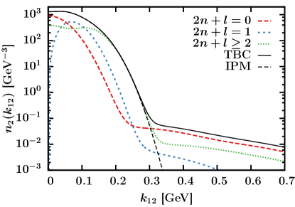
Figure 1: (Color online) The momentum dependence of the computed $n_{2}^{2n+l}(k_{12})$, $n_{2}^{\text{TBC}}(k_{12})$ and $n_{2}^{\text{IPM}}(k_{12})$ for ⁵⁶Fe in a HO basis. In order to quantify the effect of SRC we have used the $g_{c}\left(r_{12}\right)$ of Ref. Gearheart (1994) and the $f_{t\tau}\left(r_{12}\right)$, $f_{\sigma\tau}(r_{12})$ of Ref. Pieper et al. (1992).

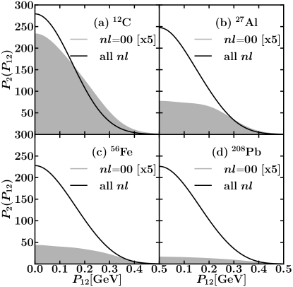
Figure 2: The momentum dependence of $P_{2}(P_{12})$ and the $P_{2}\left(P_{12}|nl=00\right)$ for pp pairs in different nuclei. The adopted normalization convention is that $\int_{0}^{\infty}\mathrm{d}P_{12}\;P_{12}^{2}P_{2}(P_{12})=1$. Note that only the pp contributions to $P_{2}(P_{12})$ are considered when performing the integral. The results are obtained in a HO basis.

Figure 3: As in Fig. 2 but for pn pairs.

In Sec. III, it is shown that in the limit of vanishing FSIs the factorization function of the exclusive $A(e,e^{\prime}pN)$ cross section is $P_{2}(P_{12}|nl=00)$. In Figs. 2 and 3, we display the computed $P_{2}(P_{12})$ and $P_{2}(P_{12}|nl=00)$ for the pp and pn pairs in ¹²C, ²⁷Al, ⁵⁶Fe and ²⁰⁸Pb. The relative weight of the $(nl=00)$ in the total c.m. distribution decreases spectacularly with increasing mass number $A$. This will reflect itself in the mass dependence of the $A(e,e^{\prime}NN)$ cross sections which are predicted to scale much softer than $A^{2}$. The $(nl=00)$ pairs are strongly localized in space which enlarges the $P_{2}(P_{12}|nl=00)$ width relative to the $P_{2}(P_{12})$ one. The mass dependence of the normalized $P_{2}(P_{12})$ reflects itself in a modest growth of the width of the distribution. For the light nuclei ¹²C and ²⁷Al, the pp and pn c.m. distributions look very similar.

At first sight the computed $P_{2}(P_{12})$ for the pp and pn pairs in Figs. 2 and 3 look very Gaussian. In what follows, we use the moments to quantify the non-Gaussianity of the $P_{2}$. The first moment, or mean, of a distribution $F(x)$ is defined as

$$\mu_{1}=\mu=\frac{\int_{D}xF(x)\mathrm{d}x}{\int_{D}F(x)\mathrm{d}x},$$ (25)

where $D$ is the domain of the distribution. For $m>1$, we define the central moments as

$$\mu_{m}=\frac{\int_{D}(x-\mu)^{m}F(x)\mathrm{d}x}{\int_{D}F(x)\mathrm{d}x}\;.$$ (26)

The width is defined as $\sigma=\sqrt{\mu_{2}}$. With regard to $\mu_{3}$ and $\mu_{4}$, it is common practice to describe a distribution with the skewness $\gamma_{1}$ and excess kurtosis $\kappa$

$$\gamma_{1} \equiv \frac{\mu_{3}}{\sigma^{3}}$$ (27)

$$\kappa \equiv \frac{\mu_{4}}{\sigma^{4}}-3,$$ (28)

which are both vanishing for a Gaussian distribution.

For a spherically symmetric distribution, one can derive the distributions $P_{2,i}\left(P_{12,i}\right)\;(i=x,y,z)$ along the axes from $P_{12}^{2}P_{2}\left(P_{12}=\sqrt{P_{12,x}^{2}+P_{12,y}^{2}+P_{12,z}^{2}}\right)$. Gaussian $P_{2,i}$ give rise to a $P_{12}^{2}P_{2}\left(P_{12,i}\right)$ of the Maxwell-Boltzmann type.

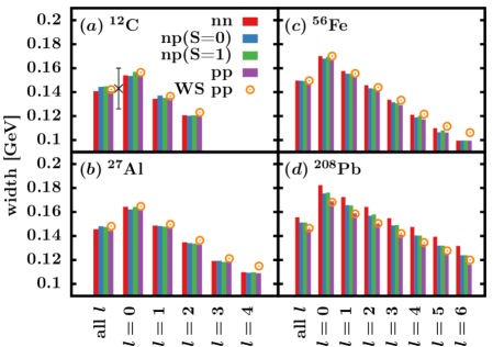
Figure 4: (Color online) Computed widths of the $P_{2,x}\left(P_{12,x}\right)$ (denoted as “all $l$”) and $P_{2,x}\left(P_{12,x}|l\right)$ distributions for pp, nn, np$(S=0)$ and np$(S=1)$ pairs in ¹²C, ²⁷Al, ⁵⁶Fe, ²⁰⁸Pb. Unless stated otherwise the results are obtained in a HO basis. For pp pairs we also display results for a WS basis (denoted as “WS pp”). The black cross is the experimental result from Ref. Tang et al. (2003).

		HO				WS
		$\sigma$ (MeV)	$\gamma_{1}$ [Eq. (27)]	$\kappa$ [Eq. (28)]		$\sigma$ (MeV)	$\gamma_{1}$ [Eq. (27)]	$\kappa$ [Eq. (28)]
12C	$P_{2,x}(P_{12,x}|nl=00)$	$156$	$0.00$	$-0.25$		$158$	$0.00$	$-0.28$
12C	$P_{2,x}(P_{12,x})$	$140$	$-0.01$	$-0.12$		$142$	$-0.01$	$-0.05$
27Al	$P_{2,x}(P_{12,x}|nl=00)$	$164$	$0.00$	$-0.45$		$168$	$0.00$	$-0.45$
27Al	$P_{2,x}(P_{12,x})$	$144$	$-0.01$	$-0.20$		$148$	$-0.01$	$-0.20$
56Fe	$P_{2,x}(P_{12,x}|nl=00)$	$172$	$0.00$	$-0.54$		$174$	$0.00$	$-0.54$
56Fe	$P_{2,x}(P_{x})$	$146$	$-0.01$	$-0.27$		$149$	$0.00$	$-0.26$
208Pb	$P_{2,x}(P_{12,x}|nl=00)$	$178$	$0.00$	$-0.58$		$177$	$0.00$	$-0.63$
208Pb	$P_{2,x}(P_{12,x})$	$145$	$0.00$	$-0.31$		$146$	$0.00$	$-0.31$

Table 1: The moments of the $P_{2,x}\left(P_{12,x}\right)$ and the $P_{2,x}\left(P_{12,x}|nl=00\right)$ distributions for pp pairs as computed in a HO and WS single-particle basis for various nuclei.

Table 1 shows the computed moments of the $P_{2,x}(P_{12,x}|nl=00)$ and $P_{2,x}(P_{12,x})$ distributions for pp pairs. These results are obtained with HO and Woods-Saxon (WS) single-particle wave functions. We find that the c.m. distributions are not perfectly Gaussian and that the non-Gaussianity grows with $A$. The values of the widths are only moderately sensitive to the single-particle basis used. The WS widths are larger by a few percent than the HO ones.

In Fig. 4, the calculated widths of the $P_{2,x}(P_{12,x})$ and $P_{2,x}(P_{12,x}|l)$ are shown for pp, nn and np pairs. For the np pairs we discriminate between singlet $(S=0)$ and triplet $(S=1)$ spin states. From Fig. 4 we draw the following conclusions. The width of the $P_{2,x}(P_{12}|l)$ depends on $l$. For $l=0$ and np pairs, the width of $P_{2,x}(P|l)$ is almost independent of $S$. For heavy nuclei there is a substantial difference in the width of the $P_{2,x}(P|l=0)$ for pp, nn and np pairs but for light nuclei this is not the case. A similar but smaller dependence on the width is found for $n$ at fixed $l$, the width of $P_{2}(P_{12}|nl)$ decreases for increasing $n$. We conclude that from the width of the c.m. distribution of the pairs one can infer information about their relative orbital momentum.

III Factorization of the two-nucleon knockout cross section

It is well known that the fivefold differential cross section for the exclusive $A(e,e^{\prime}p)A-1$ reaction under quasifree kinematics with $A-1$ spectators

$$\gamma^{*}\left(q\right)+A-1\left(p_{A-1}\right)+N\left(k_{1}\right)\longrightarrow$$

$$A-1\left(p_{A-1}\right)+N\left(p_{1}\right)\;,$$ (29)

factorizes as

$$d^{5}\sigma(e,e^{\prime}p)=K_{ep}\sigma_{ep}P_{1}(\vec{k}_{m},E_{m})\;.$$ (30)

Here, $K_{ep}$ is a kinematical factor and $\sigma_{ep}$ the off-shell electron-proton cross section. Further, $\vec{k}_{m}=-\vec{p}_{A-1}=\vec{k}_{1}$ is the missing momentum and $E_{m}=q^{0}-T_{p_{1}}-T_{A-1}$ the missing energy, whereby $T_{A-1}$ and $T_{p_{1}}$ are the kinetic energy of the recoiling nucleus and ejected nucleon. The $P_{1}(\vec{k},E)$ is the one-body spectral function and is associated with the combined probability of removing a proton with momentum $\vec{k}$ from the ground-state of $A$ and of finding the residual $A-1$ nucleus at excitation energy $E$ (measured relative to the ground-state of the target nucleus). The factorization is exact in a non-relativistic reaction model with $A-1$ spectators and vanishing FSIs Caballero et al. (1998). The validity of the spectator approximation requires that the $E_{m}$ is confined to low values, corresponding to states with a predominant one-hole character relative to the ground state of the target nucleus $A$.

Below, it is shown that also the $A(e,e^{\prime}pN)$ differential cross section factorizes under certain assumptions. The factorization function is connected to the c.m. motion of close-proximity pairs. In Ref. Frankfurt and Strikman (1988) the factorization function is introduced as the so-called decay function. In Ref. Ryckebusch (1996) a factorized expression for the $A(e,e^{\prime}pp)$ cross section has been derived. Thereby, in computing the matrix elements, all FSI effects have been neglected and the zero-range approximation $(\lim_{r_{12}\to 0})$ has been adopted. A ¹²C$(e,e^{\prime}pp)$ experiment conducted at the Mainz Microtron (MAMI) Blomqvist et al. (1998) showed very good quantitative agreement with the predicted diproton pair c.m. momentum factorization up to momenta of about 500 MeV. Here, the formalism of Ref. Ryckebusch (1996) is extended to include the effect of FSIs and to soften the zero-range approximation. Note that the limit $\lim_{r_{12}\to 0}$ effectively amounts to projecting on states with vanishing relative orbital momentum.

We consider exclusive $A(e,e^{\prime}NN)$ reactions in the spectator approximation with a virtual photon coupling to a correlated pair $N\left(k_{1}\right)N\left(k_{2}\right)$

$$\gamma^{*}\left(q\right)+A-2\left(p_{A-2}\right)+N\left(k_{1}\right)N\left(k_{2}\right)\longrightarrow$$

$$A-2\left(p_{A-2}\right)+N\left(p_{1}\right)+N\left(p_{2}\right)\;.$$ (31)

In a non-relativistic treatment, the corresponding matrix element is given by

$$\mathcal{M}^{\mu}= \int d\vec{x}_{1}\int d\vec{x}_{2}\Big{[}\chi^{\dagger}_{s_{1}}(\vec{\sigma}_{1})\xi^{\dagger}_{t_{1}}\left(\vec{\tau}_{1}\right)\chi^{\dagger}_{s_{2}}(\vec{\sigma}_{2})\xi^{\dagger}_{t_{2}}\left(\vec{\tau}_{2}\right)$$

$$\times e^{-i\vec{p}_{1}\cdot\vec{r}_{1}}e^{-i\vec{p}_{2}\cdot\vec{r}_{2}}-(1\leftrightarrow 2)\Big{]}$$

$$\times\mathcal{F}^{\dagger}_{\text{FSI}}(\vec{r}_{1},\vec{r}_{2})\hat{\mathcal{O}}^{\mu}(\vec{x}_{1},\vec{x}_{2})\phi_{\alpha_{1}}(\vec{x}_{1})\phi_{\alpha_{2}}(\vec{x}_{2})\,.$$ (32)

Here, $s_{i}(t_{i})$ are the spin (isospin) projection of the outgoing nucleons. Further, $\mathcal{F}_{\text{FSI}}(\vec{r}_{1},\vec{r}_{2})$ is an operator encoding the FSIs for a reaction where two nucleons are brought into the continuum at the spatial localizations $\vec{r}_{1}$ and $\vec{r}_{2}$ respectively. We assume that $\mathcal{F}_{\text{FSI}}$ does not depend on the spin and isospin d.o.f, which is a fair approximation at higher energies. The amplitude of Eq. (III) refers to the physical situation whereby, as a result of virtual-photon excitation, two nucleons are excited from bound states $\alpha_{1}\alpha_{2}$ into continuum states.

In Eq. (III), the effect of the correlations is implemented in the TBC approximation by means of a symmetric two-body operator Engel et al. (2011); Janssen et al. (2000)

$$\hat{\mathcal{O}}^{\mu}(\vec{x}_{1},\vec{x}_{2})=\\ \biggl{[}e^{i\vec{q}\cdot\vec{r}_{1}}\Gamma^{\mu}_{\gamma^{\star}N}(\vec{x}_{1})+e^{i\vec{q}\cdot\vec{r}_{2}}\Gamma^{\mu}_{\gamma^{\star}N}(\vec{x}_{2})\biggr{]}\hat{\mathcal{o}}\left(\vec{x}_{1},\vec{x}_{2}\right)\,,$$ (33)

where the operator $\hat{\mathcal{o}}\left(\vec{x}_{1},\vec{x}_{2}\right)$ has been defined in Eq. (21) and $\vec{q}$ is the three-momentum of the virtual photon. The $\Gamma^{\mu}_{\gamma^{\star}N}(\vec{x}_{i})$ denotes the one-body virtual photon coupling to a bound nucleon with coordinate $\vec{x}_{i}$ (includes the spatial, spin, and isospin d.o.f.). The Eq. (33) can be interpreted as the SRC-corrected photo-nucleon coupling which operates on IPM many-body wave functions.

The amplitude of Eq. (III) involves four contributions schematically shown in Fig. 5. For the sake of brevity, in the following we consider the term of Fig. 5(a) with a photon-nucleon coupling on coordinate $\vec{r}_{1}$ and the outgoing nucleon with momentum $\vec{p}_{1}$ directly attached to this vertex. The corresponding amplitude is denoted by $\mathcal{M}^{\mu}_{a}$. The other three terms in Fig. 5 follow a similar derivation.

Figure 5: The four contributions to the $A(e,e^{\prime}NN)$ amplitude of Eq. (III).

In a HO single-particle basis, one can write

$$\mathcal{M}^{\mu}_{a} =\int d\vec{r}_{1}\int d\vec{r}_{2}e^{-i(\vec{p}_{1}-\vec{q})\cdot\vec{r}_{1}}e^{-i\vec{p}_{2}\cdot\vec{r}_{2}}\mathcal{F}^{\dagger}_{\text{FSI}}(\vec{r}_{1},\vec{r}_{2})$$

$$\times \langle s_{1}t_{1},s_{2}t_{2}\mid\Gamma^{\mu}_{\gamma^{\star}N}\left(\vec{x}_{1}\right)\hat{\mathcal{o}}\left(\vec{x}_{1},\vec{x}_{2}\right)\mid\sigma_{1}\tau_{1},\sigma_{2}\tau_{2}\rangle$$

$$\times \psi_{n_{1}l_{1}m_{l_{1}}}(\vec{r}_{1})\psi_{n_{2}l_{2}m_{l_{2}}}(\vec{r}_{2})\,,$$ (34)

where $\sigma_{i}$ $(\tau_{i})$ are the spin (isospin) quantum numbers of the bound states. Further, $\psi_{n_{1}l_{1}m_{l_{1}}}$ and $\psi_{n_{2}l_{2}m_{l_{2}}}$ are the radial HO wave functions as introduced in Eq. (12).

Similar to the Eq. (13), we apply the Talmi-Moshinsky brackets $\langle|\rangle_{\text{SMB}}$ Moshinsky and Smirnov (1996) to transform Eq. (III) to relative and c.m. radial coordinates to obtain

$$\mathcal{M}^{\mu}_{a}=\sum_{\begin{subarray}{c}LM_{L}\end{subarray}}\sum_{\begin{subarray}{c}nlm_{l}\\ N\Lambda M_{\Lambda}\end{subarray}}\int d\vec{r}_{12}\int d\vec{R}_{12}e^{-i\vec{P}_{12}\cdot\vec{R}_{12}}e^{-i\vec{k}^{-}\cdot\vec{r}_{12}}\mathcal{F}^{\dagger}_{\text{FSI}}(\vec{R}_{12}+\frac{\vec{r}_{12}}{2},\vec{R}_{12}-\frac{\vec{r}_{12}}{2})\psi_{nlm_{l}}(\frac{\vec{r}_{12}}{\sqrt{2}})\psi_{N\Lambda M_{\Lambda}}(\sqrt{2}\vec{R}_{12})$$

$$\times\langle l_{1}m_{l_{1}}l_{2}m_{l_{2}}\mid LM_{L}\rangle\langle lm_{l}\Lambda M_{\Lambda}\mid LM_{L}\rangle\langle nlN\Lambda;L\mid n_{1}l_{1}n_{2}l_{2};L\rangle_{\text{SMB}}\langle s_{1}t_{1},s_{2}t_{2}\mid\Gamma^{\mu}_{\gamma^{\star}N}\left(\vec{x}_{1}\right)\hat{\mathcal{o}}\left(\vec{x}_{1},\vec{x}_{2}\right)\mid\sigma_{1}\tau_{1},\sigma_{2}\tau_{2}\rangle\;,$$ (35)

where $\vec{P}_{12}=\vec{p}_{1}+\vec{p}_{2}-\vec{q}$, $\vec{k}^{\mp}=\frac{\vec{p}_{1}-\vec{p}_{2}}{2}\mp\frac{\vec{q}}{2}$.

In Eq. (III) the sum over the relative quantum numbers is dominated by $(nl=00)$. This is based on the observation that typical correlation operators act over relatively short internucleon distances and mostly affect the $(nl=00)$ components of the $\psi_{nlm_{l}}$ wave functions. For a more detailed explanation we refer to the discussion of Fig. 1 in Sect. II and Refs. Vanhalst et al. (2011); Vanhalst et al. (2012a).

For close-proximity nucleons one can set $\vec{r}_{12}\approx\vec{0}$ in the FSI operator:

$$\mathcal{F}_{\text{FSI}}(\vec{r}_{1},\vec{r}_{2}) = \mathcal{F}_{\text{FSI}}(\vec{R}_{12}+\frac{\vec{r}_{12}}{2},\vec{R}_{12}-\frac{\vec{r}_{12}}{2})$$ (36)

$$\approx \mathcal{F}_{\text{FSI}}(\vec{R}_{12},\vec{R}_{12})\,.$$

This approximation amounts to computing the effect of FSIs as if the the two nucleons are brought into the continuum at the same spatial point (determined by the c.m. coordinate of the pair), which is very reasonable for close-proximity nucleons. With the above assumptions one arrives at the expression for the matrix element

$$\mathcal{M}^{\mu}_{a} \approx\langle s_{1}t_{1},s_{2}t_{2}\mid\widehat{\Gamma}^{\mu}_{\gamma^{\star}N}(\vec{k}^{-})\mid\sigma_{1}\tau_{1},\sigma_{2}\tau_{2}\rangle$$

$$\times \sum_{\begin{subarray}{c}N\Lambda M_{\Lambda}\end{subarray}}\langle l_{1}m_{l_{1}}l_{2}m_{l_{2}}\mid\Lambda M_{\Lambda}\rangle\langle 00N\Lambda;\Lambda\mid n_{1}l_{1}n_{2}l_{2};\Lambda\rangle_{\text{SMB}}$$

$$\times \int d\vec{R}_{12}e^{-i\vec{P}_{12}\cdot\vec{R}_{12}}\mathcal{F}^{\dagger}_{\text{FSI}}(\vec{R}_{12},\vec{R}_{12})\psi_{N\Lambda M_{\Lambda}}(\sqrt{2}\vec{R}_{12})\,,$$ (37)

with

$$\widehat{\Gamma}^{\mu}_{\gamma^{\star}N}(\vec{p})\equiv\int d\vec{r}_{12}e^{-i\vec{p}\cdot\vec{r}_{12}}\psi_{000}(\frac{\vec{r}_{12}}{\sqrt{2}})\Gamma^{\mu}_{\gamma^{\star}N}(\vec{x}_{1})\hat{\mathcal{o}}(\vec{x}_{1},\vec{x}_{2})\,.$$ (38)

In deriving the Eq. (III), we have separated the integration over the spatial and spin-isospin d.o.f.. In addition, use has been made of the fact that the operator $\hat{\mathcal{o}}(\vec{x}_{1},\vec{x}_{2})$ of Eq. (21) does not depend on the c.m. coordinate $\vec{R}_{12}$. The most striking feature of Eq. (III) is the factorization of the amplitude in a term connected to the c.m. motion of the initial pair and a term which contains the full complexity of the photon-nucleon coupling to a correlated pair.

After summing the four terms that contribute to Eq. (III) and squaring the matrix element, the eightfold differential cross section factorizes according to

$$d^{8}\sigma(e,e^{\prime}NN)=K_{eNN}\sigma_{e2N}F^{D}_{n_{1}l_{1},n_{2}l_{2}}(\vec{P}_{12}),$$ (39)

with $K_{eNN}$ a kinematic factor. Further, the off-shell electron-two-nucleon cross section is given by

$$\sigma_{e2N}\propto L_{\mu\nu}\sum_{\begin{subarray}{c}s_{1}s_{2}\sigma_{1}\sigma_{2}\\ \tau_{1}\tau_{2}\end{subarray}}J^{\mu}\left(J^{\nu}\right)^{\dagger}\,,$$ (40)

with $L_{\mu\nu}$ the leptonic tensor and $J^{\mu}$ the hadronic current given by

$$J^{\mu} =\langle s_{1}t_{1},s_{2}t_{2}\mid\widehat{\Gamma}^{\mu}_{\gamma^{\star}N}(\vec{k}^{-})\mid\sigma_{1}\tau_{1},\sigma_{2}\tau_{2}\rangle$$

$$-\langle s_{2}t_{2},s_{1}t_{1}\mid\widehat{\Gamma}^{\mu}_{\gamma^{\star}N}(\vec{k}^{+})\mid\sigma_{1}\tau_{1},\sigma_{2}\tau_{2}\rangle$$

$$+\langle s_{1}t_{1},s_{2}t_{2}\mid\widehat{\Gamma}^{\mu}_{\gamma^{\star}N}(\vec{k}^{+})\mid\sigma_{1}\tau_{1},\sigma_{2}\tau_{2}\rangle$$

$$-\langle s_{2}t_{2},s_{1}t_{1}\mid\widehat{\Gamma}^{\mu}_{\gamma^{\star}N}(\vec{k}^{-})\mid\sigma_{1}\tau_{1},\sigma_{2}\tau_{2}\rangle\,.$$ (41)

The factorization function $F^{D}_{n_{1}l_{1},n_{2}l_{2}}(\vec{P}_{12})$ in Eq. (39) can be associated with the distorted c.m. momentum distribution of pairs in a relative ($nl=00$) state of the nucleus $A$

$$F^{D}_{n_{1}l_{1},n_{2}l_{2}}(\vec{P}_{12})=4\sum_{m_{l_{1}}m_{l_{2}}}\Big{|}\sum_{N\Lambda M_{\Lambda}}\int d\vec{R}_{12}e^{-i\vec{P}_{12}\cdot\vec{R}_{12}}$$ (42)

$$\times \langle l_{1}m_{l_{1}}l_{2}m_{l_{2}}\mid\Lambda M_{\Lambda}\rangle\langle n_{1}l_{1}n_{2}l_{2};\Lambda\mid 00N\Lambda;\Lambda\rangle_{\text{SMB}}$$

$$\times \mathcal{F}^{\dagger}_{\text{ FSI}}(\vec{R}_{12},\vec{R}_{12})\psi_{N\Lambda M_{\Lambda}}(\sqrt{2}\vec{R}_{12})\Big{|}^{2}\,,$$

where the factor 4 accounts for the spin degeneracy of the HO states.

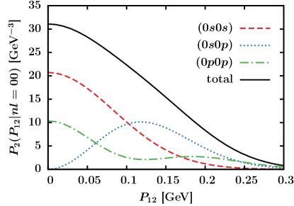
Figure 6: (Color online) The contribution of the different shell-model pair combinations to the $P_{2}\left(P_{12}|nl=00\right)$ for pp pairs in ¹²C.

In the limit of vanishing FSIs ($\mathcal{F}_{\text{ FSI}}\equiv 1$), one has

$$P_{2}(P_{12}|nl=00)=\frac{1}{A(A-1)}\frac{3}{(2\pi)^{3}}\\ \times\sum_{n_{\alpha}l_{\alpha}n_{\beta}l_{\beta}}\int d\Omega_{P_{12}}F^{D}_{n_{\alpha}l_{\alpha},n_{\beta}l_{\beta}}(\vec{P}_{12})\;.$$ (43)

This establishes a connection between the $A(e,e^{\prime}NN)$ factorization function and the contribution of pairs with quantum numbers $(n_{1}l_{1}n_{2}l_{2})$ to $P_{2}(P_{12}|nl=00)$, illustrated for pp pairs in ¹²C in Fig. 6.

In the naive IPM, each two-hole (2h) state $(n_{1}l_{1})^{-1}(n_{2}l_{2})^{-1}$ can be associated with a sharp excitation energy in the $A-2$ system. In reality, the 2h strength corresponding with $(n_{1}l_{1})^{-1}(n_{2}l_{2})^{-1}$ extends over a wide energy range Barbieri et al. (2004). Current $A(e,e^{\prime}pN)$ measurements are performed at $Q^{2}$-values of the order of GeV² not allowing one to measure cross sections for real exclusive processes as could be done at lower $Q^{2}$ values Starink et al. (2000); Ryckebusch and Van Nespen (2004); Middleton et al. (2010). Accordingly, rather than probing the individual 2h contributions to $P_{2}$, the measured semi-inclusive $A(e,e^{\prime}pN)$ cross sections can be linked to the $P_{2}(P_{12}\mid nl=00)$ which involves a summation over the 2h states. From Fig. 6 it can be appreciated that in high-resolution $A(e,e^{\prime}pN)$ measurements the c.m. distribution depends on the two-hole structure of the discrete final A-2 state Ryckebusch and Van Nespen (2004); Barbieri et al. (2004).

The $A(e,e^{\prime}p)$ reaction allows one to access the $P_{1}(\vec{k}_{m},E_{m})$ modulo corrections from FSIs. It is worth stressing that there is no simple analogy for the $A(e,e^{\prime}pN)$ reaction and that a direct connection with the two-body spectral function $P_{2}(\vec{P}_{12},\vec{k}_{12},E_{2m})$ is by no means evident, if not impossible.

IV Monte Carlo simulations

In this section, we investigate the implications of the proposed factorization of Eq. (39) for the $A(e,e^{\prime}pp)$ opening-angle and c.m. distributions accessible in typical measurements. We present Monte Carlo simulations for $A(e,e^{\prime}pp)$ building on the expression (39) suggesting that the magnitude of the cross section is proportional to $P_{2}(P_{12}|nl=00)$. In this section the effects of FSIs are neglected. Its impact will be the subject of Sect. V.

The data-mining effort at CLAS in Jlab Weinstein et al. (2009); Hen et al. (2013) is analyzing exclusive $(e,e^{\prime}pN)$ for ¹²C, ²⁷Al, ⁵⁶Fe, and ²⁰⁸Pb for a 5.014 GeV unpolarized electron beam Weinstein et al. (2009). In order to guarantee the exclusive character of the events, cuts are applied to the leading proton: $0.62<\frac{|\vec{p}_{1}|}{|\vec{q}|}<0.96$, $\theta_{\vec{p}_{1},\vec{q}}<$25\text{\,}\mathrm{\SIUnitSymbolDegree}$$ and $k_{1}>$300\text{\,}\mathrm{MeV}$$. To increase the sensitivity to SRC-driven processes one imposes the kinematic constraints $x_{B}=\frac{Q^{2}}{2M_{N}\omega}>1.2$ and $Q^{2}>1.4$ GeV². We have performed $(e,e^{\prime}pp)$ simulations for all 4 target nuclei. The electron kinematics are drawn from the measured $x_{B}-Q^{2}$ distributions. We then generate two protons from the phase space by adoping a reaction picture of the type (III) whereby we assume that one nucleon absorbs the virtual photon. This results in a fast leading proton $p_{1}(E_{1},\vec{p}_{1}=\vec{k}_{1}+\vec{q})$ and a recoil proton $p_{2}(E_{2},\vec{p}_{2}=\vec{k}_{2})$, where $\vec{k}_{1}$ and $\vec{k}_{2}$ are the initial proton momenta. The initial c.m. momentum $\vec{P}_{12}=\vec{k}_{1}+\vec{k}_{2}$ is drawn from the computed HO pp pair c.m. momentum distribution $P_{2}(P_{12}|nl=00)$ of Table 1. We choose $\vec{k}_{1}$ along the $z$-axis and $\vec{q}$ in the $xz$ plane. The recoil $A-2$ nucleus can have excitation energies between $0$ and $80$ MeV. All $A(e,e^{\prime}pp)$ results of this section are obtained for $10^{5}$ events which comply with the kinematic cuts.

First, we investigate in how far the factorization function can be addressed after applying kinematic cuts. This can be done by comparing the input and extracted pp c.m. distributions. Fig. 7 shows the extracted c.m. distribution from the simulated ¹²C$(e,e^{\prime}pp)$ events. The kinematic cuts have a narrowing effect (less than 10 %) on the distributions along the $x$- and $y$-axis. In addition, one observes a shift of roughly $100$ MeV and an increase in the non-Gaussianity of the c.m. distribution along the $z$-axis. Similar observations have been made for the other three target nuclei.

We now address the issue whether the extracted c.m. distributions can provide information about the relative quantum numbers of the pairs. To this end, we have performed simulations starting from the assumption that the $(e,e^{\prime}pp)$ cross section factorizes with $P_{2}(P_{12}|nl)$ for various $nl$ combinations. The results of the simulations are summarized in Table 2. The narrowing effect attributed to the kinematic cuts is less significant for $l>0$ pairs. Photon absorption on $l=0$ and $l=1$ pairs leads to differences in the extracted widths of the c.m. momentum distributions of the order of 20 MeV, which leads us to conclude that high-accuracy $A(e,e^{\prime}pp)$ experiments could indeed provide information about the relative orbital angular momentum of the correlated pairs.

Fig. 8 shows the simulated opening-angle ($\gamma$) distributions of the initial-state protons for all four target nuclei considered. The A$(e,e^{\prime}pp)$ simulations starting from the computed $P_{2}(P_{12}|nl=00)$ and $P_{2}(P_{12})$ provide very similar backwardly peaked $\cos\gamma$ distributions. The peak is not due to the kinematic cuts as a uniform c.m. momentum distributions gives rise to a flat $\cos\gamma$ distribution. The shape of the simulated $\cos\gamma$ distributions is hardly target-mass dependent. The peak at 180 degrees in the $\cos\gamma$ distributions conforms with the picture of correlated nucleons moving back to back with high relative and low c.m. momentum.

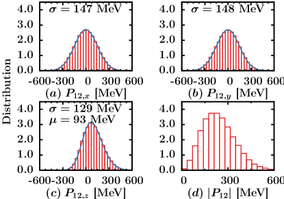
Figure 7: (Color online) Total (bottom right) and directional pp c.m. distributions extracted from the ¹²C$(e,e^{\prime}pp)$ simulations in the CLAS kinematics described in the text. The blue solid line is a fit with a skew normal distribution.

	$nl=00$	$l=0$	$l=1$	$l=2$	all $l$
$\sigma_{x}^{i}(MeV)$	$156$	$154$	$135$	$121$	$140$
$\sigma_{x}^{f}(MeV)$	$147$	$145$	$130$	$118$	$134$

Table 2: The width of the c.m. distribution along the $x$-axis for pp pairs with different relative orbital momentum $l$. $\sigma_{x}^{i}$ is the width used as input parameter in the ¹²C$(e,e^{\prime}pp)$ simulations. The $\sigma_{x}^{f}$ is the width extracted after the simulation.

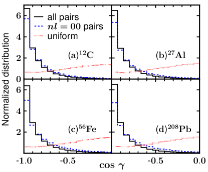
Figure 8: (Color online) The opening angle distribution of the simulated A$(e,e^{\prime}pp)$ events in the kinematics described in the text. The black solid, blue dashed and red dotted line is for a reaction picture with an $(e,e^{\prime}pp)$ cross section proportional to $P_{2}(P_{12})$, to $P_{2}(P_{12}|nl=00)$, and to a uniform pair c.m. distribution.

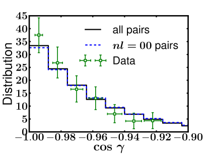
Figure 9: (Color online) The opening angle distribution of the ¹²C$(e,e^{\prime}pp)$ reaction in the kinematics of Ref. Shneor et al. (2007). Curve notations of Fig. 8 are used.

We now turn our attention to an ¹²C$(e,e^{\prime}pp)$ measurement probing a restricted part of phase space. The JLab Hall-A ¹²C($e,e^{\prime}pp$) experiment of Refs. Shneor et al. (2007); Subedi et al. (2008), used an incident electron beam of $4.672$ GeV and three spectrometers. We consider the kinematic settings with $\omega=0.865$ GeV, $Q^{2}=2$ GeV², $x_{B}=1.2$ and a median missing momentum $p_{m}=0.55$ GeV. Figure 9 shows the shapes of the simulated and measured $\cos\gamma$ simulations. The proposed factorization for the $A(e,e^{\prime}pp)$ cross section accounts for the shape of the measured $\cos\gamma$ distribution. We stress that the computed pair c.m. distributions (Table 1) are the sole input to the simulations.

V FINAL STATE INTERACTIONS

In this section the impact of FSIs on the proposed factorization function of Eq. (39) is investigated. In order to keep computing times reasonable we limit ourselves to some particular kinematic cases and introduce an additional approximation. We start from Eq. (42) for the distorted momentum distribution $F^{D}_{n_{1}l_{1},n_{2}l_{2}}(\vec{P}_{12})$ and apply the zero-range approximation Ryckebusch (1996); Cosyn and Ryckebusch (2009) which amounts to setting $\psi_{\alpha_{1}}(\vec{r}_{1})\psi_{\alpha_{2}}(\vec{r}_{2})\approx\psi_{\alpha_{1}}(\vec{R}_{12})\psi_{\alpha_{2}}(\vec{R}_{12})$ in Eq. (III). Consequently, we can write

$$F^{D}_{n_{1}l_{1},n_{2}l_{2}}(\vec{P}_{12})=4\sum_{m_{l_{1}}m_{l_{2}}}\Big{|}\int d\vec{R}_{12}e^{-i\vec{P}_{12}\cdot\vec{R}_{12}}\\ \times\mathcal{F}^{\dagger}_{\text{ FSI}}(\vec{R}_{12},\vec{R}_{12})\psi_{n_{1}l_{1}m_{l_{1}}}(\vec{R}_{12})\psi_{n_{2}l_{2}m_{l_{2}}}(\vec{R}_{12})\Big{|}^{2}\,.$$ (44)

It is possible to derive a relativized version of this expression Cosyn and Ryckebusch (2009)

$$F^{D}_{n_{1}\kappa_{1},n_{2}\kappa_{2}}(\vec{P}_{12})=\\ \sum_{s_{1},s_{2},m_{1},m_{2}}\left|\int d\vec{R}_{12}\,e^{i\vec{P}_{12}\cdot\vec{R}_{12}}\mathrm{bar}{u}(\vec{k}_{1},s_{1})\psi_{n_{1}\kappa_{1}m_{1}}(\vec{R}_{12})\right.\\ \left.\mathrm{bar}{u}(\vec{k}_{2},s_{2})\psi_{n_{2}\kappa_{2}m_{2}}(\vec{R}_{12})\mathcal{F}_{\text{FSI}}(\vec{R}_{12},\vec{R}_{12})\right|^{2}\,.$$ (45)

Here, $u(\vec{k},s)$ are positive-energy Dirac spinors and $\psi_{n\kappa m}$ are relativistic mean-field wave functions Furnstahl et al. (1997) with quantum numbers $(n,j=|\kappa|/2,m)$. We neglect the projections on the lower components of the plane-wave Dirac spinors. The FSIs of the ejected pair with the remaining $A-2$ spectators, encoded in $\mathcal{F}_{\text{FSI}}$, can be computed in a relativistic multiple-scattering Glauber approximation (RMSGA) Ryckebusch et al. (2003); Cosyn and Ryckebusch (2013). As the c.m. momentum is conserved in interactions among the two ejected nucleons, we discard those. This approximation does not affect the shape of $F^{D}_{n_{1}\kappa_{1},n_{2}\kappa_{2}}(\vec{P}_{12})$.

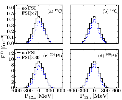
Figure 10: (Color online) The two-body c.m. momentum distribution for ${}^{12}\text{C}(e,e^{\prime}pp)$ (top) and ${}^{208}\text{Pb}(e,e^{\prime}pp)$ (bottom) with (RMSGA) and without (no-FSI) inclusion of FSIs. We consider the kinematics $|\vec{q}|=1.4~{}\text{GeV},|\vec{p}_{1}|=0.82|\vec{q}|$ and $\theta_{\vec{p}_{1},\vec{q}}=10^{\circ}$. The FSI results have been multiplied by a factor of $7$ for ${}^{12}\text{C}(e,e^{\prime}pp)$ and by a factor of $30$ for ${}^{208}\text{Pb}(e,e^{\prime}pp)$.

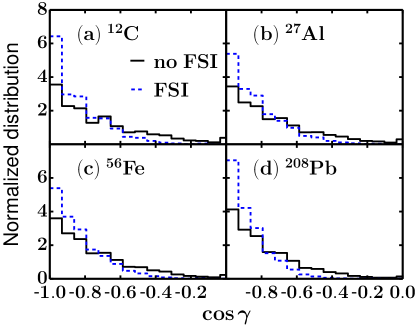
Figure 11: (Color online) The normalized opening angle distributions for A$(e,e^{\prime}pp)$ for ¹²C, ²⁷Al, ⁵⁶Fe and ²⁰⁸Pb in the kinematics of Fig. 10.

We include FSIs for the JLab data mining kinematics considered in Sec. IV. We have computed the distorted c.m. momentum distribution of Eq. (45) for the kinematics that yields the most events in the simulations of Sec. IV: $|\vec{q}|=1.4~{}\text{GeV},|\vec{p}_{1}|=0.82|\vec{q}|,\theta_{\vec{p}_{1},\vec{q}}=10^{\circ}$. As in Sec. IV, $\vec{k}_{1}$ lies along the $z$-axis and the $\vec{q}$ is located in the $xz$ plane. The results of the FSI calculations are summarized in Figs. 10 and 11.

In Fig. 10 we compare the RMSGA c.m. momentum distributions $F^{D}(\vec{P}_{12,x})=\sum_{n_{1}\kappa_{1},n_{2}\kappa_{2}}F^{D}_{n_{1}\kappa_{1},n_{2}\kappa_{2}}(\vec{P}_{12,x})$ and $F^{D}(\vec{P}_{12,y})$ with their respective plane-wave (no-FSI) limit. First, the FSIs are responsible for a substantial reduction of the cross sections: a factor of about 7 for carbon and about 30 in lead. The effects of FSIs on the shape of $F^{D}(\vec{P}_{12})$, however, are rather modest. Gaussian fits to the $F^{D}(\vec{P}_{12,i=x,y})$ result in widths which are less than 10% smaller than in the plane-wave limit. The effects of FSIs on the shape of the c.m. distributions in Fig. 10 can be qualitatively understood considering that the nucleons undergoing FSIs are slowed down on average: $(\vec{p}_{1},\vec{p}_{2})\xrightarrow{\text{FSI}}\zeta\left(\vec{p}_{1},\vec{p}_{2}\right)$ with $0<\zeta\leq 1$. It is straightforward to show that for the adopted conventions this results in $P_{12,x}\rightarrow\zeta P_{12,x}-(1-\zeta)p_{1,x}$, and $P_{12,y}\rightarrow\zeta P_{12,y}$. This explains the observed contraction and shift to the right in the $P_{12,x}$ distribution, and the contraction of the $P_{12,y}$ distributions.

The effect of FSIs on the shape of the normalized opening angle distributions is studied in Fig. 11 for four target nuclei. It is clear that they become even more forwardly peaked after including FSIs.

VI Summary

Summarizing, we have shown that in the plane-wave limit the factorization function for the exclusive SRC-driven $A(e,e^{\prime}pN)$ reaction is the conditional c.m. distribution $P_{2}(P_{12}|nl=00)$ for pN pairs in a nodeless relative state with a vanishing orbital momentum. We have illustrated that in a two-body cluster expansion the correlated part of the momentum distribution originates mainly from correlation operators acting on IPM pairs with $(nl=00)$ quantum numbers, supporting the assumptions underlying the proposed factorization of the $A(e,e^{\prime}pN)$ reaction. Numerical calculations indicate that the $P_{2}(P_{12}|nl=00)$ has a wider distribution than the unconditional $P_{2}(P_{12})$ one. An important implication of the proposed factorization is that the mass dependence of the $A(e,e^{\prime}pp)$ and $A(e,e^{\prime}pn)$ cross section is predicted to be much softer than $\frac{Z(Z-1)}{2}$ and $NZ$ respectively.

We have examined the robustness of the proposed factorization of the two-nucleon knockout cross sections against kinematic cuts and FSIs. Both mechanisms modestly affect the shape of the c.m. distributions which leads us to conclude that they can be accessed in $A(e,e^{\prime}pN)$ measurements. The FSIs bring about a mass-dependent reduction of the cross sections which is of the order of 10 for carbon and 30 for lead.

ACKNOWLEDGMENTS

The authors wish to thank Or Hen, Eli Piasetzky, and Larry Weinstein for stimulating discussions and suggestions. This work is supported by the Research Foundation Flanders (FWO-Flanders) and by the Interuniversity Attraction Poles Programme P7/12 initiated by the Belgian Science Policy Office. The computational resources (Stevin Supercomputer Infrastructure) and services used in this work were provided by Ghent University, the Hercules Foundation and the Flemish Government.

References

Tang et al. (2003)
A. Tang,
J. W. Watson,
J. Aclander,
J. Alster,
G. Asryan,
Y. Averichev,
D. Barton,
V. Baturin,
N. Bukhtoyarova,
A. Carroll,
et al., Phys. Rev. Lett.
90, 042301
(2003).
Niyazov et al. (2004)
R. A. Niyazov,
L. B. Weinstein,
G. Adams,
P. Ambrozewicz,
E. Anciant,
M. Anghinolfi,
B. Asavapibhop,
G. Asryan,
G. Audit,
T. Auger, et al.
(CLAS Collaboration), Phys. Rev.
Lett. 92, 052303
(2004).
Shneor et al. (2007)
R. Shneor,
P. Monaghan,
R. Subedi,
B. D. Anderson,
K. Aniol,
J. Annand,
J. Arrington,
H. Benaoum,
F. Benmokhtar,
P. Bertin,
et al. (Jefferson Lab Hall A
Collaboration), Phys. Rev. Lett.
99, 072501
(2007).
Subedi et al. (2008)
R. Subedi,
R. Shneor,
P. Monaghan,
B. Anderson,
K. Aniol,
J. Annand,
J. Arrington,
H. Benaoum,
F. Benmokhtar,
W. Boeglin,
et al., Science
320, 1476 (2008).
Egiyan et al. (2003)
K. S. Egiyan,
N. Dashyan,
M. Sargsian,
S. Stepanyan,
L. B. Weinstein,
G. Adams,
P. Ambrozewicz,
E. Anciant,
M. Anghinolfi,
B. Asavapibhop,
et al. (CLAS Collaboration),
Phys. Rev. C 68,
014313 (2003).
Egiyan et al. (2006)
K. S. Egiyan,
N. B. Dashyan,
M. M. Sargsian,
M. I. Strikman,
L. B. Weinstein,
G. Adams,
P. Ambrozewicz,
M. Anghinolfi,
B. Asavapibhop,
G. Asryan,
et al. (CLAS Collaboration),
Phys. Rev. Lett. 96,
082501 (2006).
Fomin et al. (2012)
N. Fomin,
J. Arrington,
R. Asaturyan,
F. Benmokhtar,
W. Boeglin,
P. Bosted,
A. Bruell,
M. H. S. Bukhari,
M. E. Christy,
E. Chudakov,
et al., Phys. Rev. Lett.
108, 092502
(2012).
Schiavilla et al. (2007)
R. Schiavilla,
R. B. Wiringa,
S. C. Pieper,
and J. Carlson,
Phys. Rev. Lett. 98,
132501 (2007).
Wiringa et al. (2008)
R. B. Wiringa,
R. Schiavilla,
S. C. Pieper,
and J. Carlson,
Phys. Rev. C 78,
021001 (2008).
Feldmeier et al. (2011)
H. Feldmeier,
W. Horiuchi,
T. Neff, and
Y. Suzuki,
Phys. Rev. C 84,
054003 (2011).
Wiringa et al. (2013)
R. Wiringa,
R. Schiavilla,
S. C. Pieper,
and J. Carlson
(2013), eprint 1309.3794.
Alvioli et al. (2008)
M. Alvioli,
C. Ciofi degli Atti,
and H. Morita,
Phys. Rev. Lett. 100,
162503 (2008).
Alvioli et al. (2012)
M. Alvioli,
C. Ciofi degli Atti,
L. P. Kaptari,
C. B. Mezzetti,
H. Morita, and
S. Scopetta,
Phys. Rev. C 85,
021001 (2012).
Alvioli et al. (2013)
M. Alvioli,
C. Ciofi degli Atti,
L. P. Kaptari,
C. B. Mezzetti,
and H. Morita,
Phys. Rev. C 87,
034603 (2013).
Arias de Saavedra et al. (2007)
F. Arias de Saavedra,
C. Bisconti,
G. Co’, and
A. Fabrocini,
Phys.Rept. 450,
1 (2007).
Bisconti et al. (2007)
C. Bisconti,
F. A. d. Saavedra,
and G. Co’,
Phys. Rev. C 75,
054302 (2007).
Bogner and Roscher (2012)
S. Bogner and
D. Roscher,
Phys. Rev. C86,
064304 (2012).
Arrington
et al. (2012a)
J. Arrington,
D. Higinbotham,
G. Rosner, and
M. Sargsian,
Prog. Part. Nucl. Phys. 67,
898 (2012a).
Frankfurt et al. (2008)
L. Frankfurt,
M. Sargsian, and
M. Strikman,
Int. J. Mod. Phys. A23,
2991 (2008).
Vanhalst et al. (2011)
M. Vanhalst,
W. Cosyn, and
J. Ryckebusch,
Phys. Rev. C84,
031302 (2011).
Vanhalst
et al. (2012a)
M. Vanhalst,
J. Ryckebusch,
and W. Cosyn,
Phys. Rev. C86,
044619 (2012a).
Vanhalst
et al. (2012b)
M. Vanhalst,
J. Ryckebusch,
and W. Cosyn
(2012b), eprint 1210.6175.
Cosyn et al. (2013)
W. Cosyn,
M. Vanhalst, and
J. Ryckebusch
(2013), eprint 1308.5583.
Arrington
et al. (2012b)
J. Arrington,
A. Daniel,
D. Day,
N. Fomin,
D. Gaskell,
et al., Phys. Rev.
C86, 065204
(2012b).
Benhar (2013)
O. Benhar,
Phys. Rev. C 87, 024606
(2013).
Starink et al. (2000)
R. Starink,
M. van Batenburg,
E. Cisbani,
W. Dickhoff,
S. Frullani,
F. Garibaldi,
C. Giusti,
D. Groep,
P. Heimberg,
W. Hesselink,
et al., Phys.Lett.
B474, 33 (2000).
Moshinsky and Smirnov (1996)
M. Moshinsky and
Y. Smirnov,
The harmonic oscillator in modern physics
(Harwood Academic Publishers,Amsterdam,
1996).
Pieper et al. (1992)
S. C. Pieper,
R. B. Wiringa,
and
V. Pandharipande,
Phys. Rev. C 46,
1741 (1992).
Engel et al. (2011)
J. Engel,
J. Carlson, and
R. Wiringa,
Phys. Rev. C83,
034317 (2011).
Roth et al. (2010)
R. Roth,
T. Neff, and
H. Feldmeier,
Prog. Part. Nucl. Phys. 65,
50 (2010).
Janssen et al. (2000)
S. Janssen,
J. Ryckebusch,
W. Van Nespen,
and D. Debruyne,
Nucl. Phys. A 672,
285 (2000).
Ryckebusch et al. (1997)
J. Ryckebusch,
V. Van der Sluys,
K. Heyde,
H. Holvoet,
W. Van Nespen,
M. Waroquier,
and
M. Vanderhaegen,
Nucl. Phys. A 624,
581 (1997).
Gearheart (1994)
C. Gearheart, Ph.D. thesis,
Washington University, St. Louis
(1994).
Caballero et al. (1998)
J. Caballero,
T. Donnelly,
E. Moya de Guerra,
and J. Udias,
Nucl. Phys. A632,
323 (1998).
Frankfurt and Strikman (1988)
L. L. Frankfurt
and M. I.
Strikman, Phys. Rept.
160, 235 (1988).
Ryckebusch (1996)
J. Ryckebusch,
Phys. Lett. B383,
1 (1996).
Blomqvist et al. (1998)
K. I. Blomqvist
et al., Phys. Lett.
B421, 71 (1998).
Barbieri et al. (2004)
C. Barbieri,
C. Giusti,
F. Pacati, and
W. Dickhoff,
Phys. Rev. C70,
014606 (2004).
Ryckebusch and Van Nespen (2004)
J. Ryckebusch and
W. Van Nespen,
Eur. Phys. J. A20,
435 (2004).
Middleton et al. (2010)
D. Middleton,
J. Annand,
C. Barbieri,
C. Giusti,
P. Grabmayr,
et al., Eur. Phys. J.
A43, 137 (2010).
Weinstein et al. (2009)
L. Weinstein,
S. Kuhn, et al.,
Short distance structure of nuclei: Mining the wealth of
existing jefferson lab data, DOE Grant DE-SC0006801 (2009).
Hen et al. (2013)
O. Hen et al.
(CLAS Collaboration), Phys. Lett.
B722, 63 (2013).
Cosyn and Ryckebusch (2009)
W. Cosyn and
J. Ryckebusch,
Phys. Rev. C80,
011602 (2009).
Furnstahl et al. (1997)
R. J. Furnstahl,
B. D. Serot, and
H.-B. Tang,
Nucl. Phys. A615,
441 (1997).
Ryckebusch et al. (2003)
J. Ryckebusch,
D. Debruyne,
P. Lava,
S. Janssen,
B. Van Overmeire,
and
T. Van Cauteren,
Nucl. Phys. A728,
226 (2003).
Cosyn and Ryckebusch (2013)
W. Cosyn and
J. Ryckebusch,
Phys. Rev. C 87, 064608
(2013).