A space-time stochastic model and a covariance function for the stationary spatio-temporal random process and spatio-temporal prediction (kriging)

Abstract

Consider a stationary spatio-temporal random process $\{Y_{t}(\mathbf{s})\mathbf{|s}\in\mathbb{R}^{d},$ $\ t\in\mathbb{Z\}}$ and let $\{Y_{t}(\mathbf{s}_{i})\mathbf{|}i=1,2,...m;\ t=1,\ldots,n$ $\mathbb{\}}$ be a sample from the random process$\ \{Y_{t}\left(\mathbf{s}\right)\mathbf{\}}$. Our object here is to estimate $\{Y_{t}(\mathbf{s}_{o)}\}$ for all $t$ at the location $\mathbf{s}_{o}$ given the sample $\{Y_{t}(\mathbf{s}_{i})|\ i=1,2,...m;\ t=1,\ldots,n\mathbf{\}}$ using the frequency domain approach. To obtain an estimator, we define a sequence of Discrete Fourier transforms $\{J_{\mathbf{s}}(\omega_{i})\}$ at  the Fourier frequencies using the time series observed at the locations $\mathbf{s}_{i},$ $\left(i=1,2,3...m\right)$, and use these complex random variables as our observations from the complex valued random process $\{J_{\mathbf{s}}(\omega)\}$. The  Fourier transforms are functions of the spatial coordinates only. Assuming the complex valued process satisfies a complex stochastic partial differential equation (CSPDE) of the Laplacian type, and using the properties of Fourier transforms of stationary processes, we obtain an expression for the spatio-temporal covariance function and  for the spectral density function. The covariance function of the Discrete Fourier transforms at two distinct locations has been shown to be a function of the Euclidean  distance and the temporal frequency  and its second order spectrum corresponds to non separable class of random processes. We show further that the model defined here includes as special cases the spatio-temporal models defined by [11], [12] and [20]. The estimation  of the parameters of the spatio-temporal covariance function  has also been considered. The method of estimation is based on Frequency Variogram approach recently introduced and it does not involve inversion of large dimensional matrices and found to be robust against departure from Gaussianity. Since the methods developed here are based on the Discrete Fourier Transforms, and  these transforms can be evaluated using Fast Fourier Transform algorithms, the estimation methods are quick and efficient compared to the classical approaches based on Variogram method and the likelihood approaches. The methods are illustrated with a real example. The data considered is Air Pollution data (Particulate Matter PM_2.5) recorded at 15 locations in New York city observed over a period of 9 months and the data at the location 11 has large number of missing values. The data at this location is estimated and prediction intervals are given and the estimates are compared with the observed data when the data is available.

Keywords:  Complex Stochastic Partial Differential Equations, Covariance Functions, Discrete Fourier Transforms, Spatio-Temporal Processes, Prediction (Kriging), Frequency Variogram.

1 Introduction and Summary

In recent years it has become necessary to develop statistical methods for the analysis of data coming from diverse areas such as, environment, marine biology, agriculture, finance etc. The data which comes from these areas, are usually, functions of both space and time. Any statistical method developed must take into account  both spatial dependence, temporal dependence and any interaction between space and time. There is a vast literature on statistical analysis of stationary spatial data (for example refer to the books of [4], [22]) but not  to the same extent in the case of stationary spatio-temporal data. The inclusion of an extra temporal dimension, which cannot be imbedded into spatial dimension gives raise to many problems. One such problem is finding a suitable covariance function  which is positive definite and depends on spatial lag difference and temporal lag. In recent years several authors (see [5], [10], [7], [23], [3], [11], [13], [14], [12], and [20]) have proposed various types of covariance functions, and majority of them are Matern type of functions. [11], [12] and [20] have considered transport-diffusion Stochastic Partial Differential (SPDE) equations for modelling of stationary spatio-temporal random process. The models  defined by these authors are stochastic versions of the  classical Heat equation, which is in fact a dynamic form of the Laplace equation, and the temporal correlation is explained by inclusion of a first order time derivative. In a way this is equivalent to assuming that always the temporal correlation in the data can be explained by a first order Autoregressive model(AR(1)). This assumption some times can be very unrealistic. [12] considered the approximation of Gaussian Field (GF) models by the Gaussian  Markov Random Field (GMRF) models and considered modelling the data by GMRF models. [20] have approximated the solution of the SPDE models by a linear combination of deterministic spatial functions (Fourier functions  in terms of spatial wave numbers) with random coefficients that evolve dynamically and requires discretization  in time for application to  discrete time series.

The prediction of the data at a known location (usually known as Kriging) is another important problem. The object here is to predict the data at a known location where the time series data is not observed. It is well known that the best linear minimum mean square predictor depends on the unknown  covariance function of the process . The elements of  the variance covariance matrix cannot be estimated from the data as no data is available at the location where we are estimating the data. Therefore, there is a need to find a suitable parametric covariance function. Our main object in this paper is to explore and investigate possible ways of using the Discrete Fourier Transforms of spatio-temporal data in modelling and prediction(for further applications of the DFT to spatial data analysis, we refer to [27]. We use many well known asymptotic sampling properties of the Discrete Fourier Transforms of stationary time series in our derivations.

The novel features of our present paper are as follows. We consider the discrete Fourier transforms of the given spatio-temporal data and treat these complex Gaussian variables as our data. We define the complex Gaussian process through a stochastic partial differential equation in spatial coordinates only. By defining in this way and operating on the Fourier transforms, the dependency of the operator on time is removed and hence no discretization in time is necessary. By analyzing the Complex Gaussian processes and using the defined Complex Stochastic Partial Differential Equations (CSPDE), we are reducing the number of computations required for solving the equations, the estimation of the parameters of the covariance function and for forecasting too. Under the assumption of isotropy, we obtain an expression for the covariance of the Discrete Fourier Transforms at different locations in terms of the Euclidean distance between the locations, and it is shown to be in terms of the modified Bessel function (Matern Class).The covariance function obtained here is a function of the Euclidean spatial distance, and the temporal frequency spectrum characterising the temporal dependence in the series In this way the expression for the covariance function given here is fundamentally different from other covariance functions defined and used by other authors. We further show that the  second order spectral density function of the spatio-temporal random process defined here through the above operator on the discrete Fourier transforms includes all the second order spectra of the process so far defined  through the stochastic versions of the Laplace equation such as, Heat equation (transport-diffusion equation of [11], [12] and [20]), Wave equation and Helmholtz equation as special cases. The second order spectral density function obtained here belongs to nonseparable random process.

We summarize the contents of each section. In section 2, the notation and the spectral representation of the spatio-temporal random process  are introduced. The properties of  the Discrete Fourier transforms of second order stationary processes are discussed in the appendix. Expressions for the spatio-temporal covariance and for the spectral density functions when the Discrete Fourier Transforms satisfy a Complex Stochastic Partial Differential equation (CSPDE) are obtained in section 3. We also show in this section that the second order spectra of the processes satisfying the models defined by [11],  and [20] can be obtained as special cases of the CSPDE model defined here. The main results related to the process satisfying CSPDE are stated in theorems 1 and 2. The prediction of the entire data at a known location given the data in the neighborhood using the Discrete Fourier transforms is considered in section 4. The estimation of the parameters, using Frequency Variogram method,  of the spatio-temporal covariance function is considered in section 5. In section 6, the analysis of the Air Pollution data (Particulate Matter PM_2.5) collected at 15 locations in New York City is considered. The prediction of the entire data at the location 11, where large number of observations are missing  is also considered in section 6 and the plots of the estimated data together with prediction intervals are also given. The estimates of the observations corresponding to PM_2.5  at time $t=22$  and at all the 625 locations (the spatial coordinates are known) are calculated and the surface plot of the estimated values is shown in Fig 4 of section 6.

2 Notation and Preliminaries

Let $Y_{t}\left(\mathbf{s}\right)$, where $\left\{\mathbf{s}\in\mathbb{R}^{d},t\in\mathbb{Z}\right\}$, denote the spatio-temporal random process. We assume that the random process is spatially and temporally second order stationary, i.e.

$$E\left[Y_{t}\left(\mathbf{s}\right)\right] =\mu,$$

$$Var\left[Y_{t}\left(\mathbf{s}\right)\right] =\sigma_{Y}^{2}<\infty,$$

$$Cov\left[Y_{t}\left(\mathbf{s}\right),Y_{t+u}\left(\mathbf{s}+\mathbf{h}\right)\right] =c\left(\mathbf{h},u\right),\quad\mathbf{h}\in\mathbb{R}^{d},\,u\in\mathbb{Z}\mathbf{.}$$

We note that $c\left(\mathbf{h},0\right)$ and $c\left(\mathbf{0},u\right)$ correspond to the purely spatial and purely temporal covariances of the process respectively. A further common stronger assumption that is often made is that the process  is isotropic. The assumption of isotropy is a stronger assumption. The process is said to be isotropic if

$$c\left(\mathbf{h},u\right)=c\left(\left\|\mathbf{h}\right\|,u\right),\quad\left\|\mathbf{h}\right\|\geq 0,\,u\in\mathbb{Z},$$

where $\left\|\mathbf{h}\right\|$ is the Euclidean distance. Without loss of generality, we set $\mu$ equal to zero. As in the case of spatial process, one can define the spatio-temporal variogram for $\left\{Y_{t}\left(\mathbf{s}\right)\right\}$ as

$$2\gamma\left(\mathbf{h},u\right)=Var\left[Y_{t+u}\left(\mathbf{s}+\mathbf{h}\right)-Y_{t}\left(\mathbf{s}\right)\right].$$ (1)

If the random process $\left\{Y_{t}\left(\mathbf{s}\right)\right\}$ is spatially and temporally stationary, then we can rewrite the above as

$$2\gamma\left(\mathbf{h},u\right)=2\left[c\left(\mathbf{0},0\right)-c\left(\mathbf{h},u\right)\right],$$ (2)

and for an isotropic process, $\gamma\left(\mathbf{h},u\right)=\gamma\left(\left\|\mathbf{h}\right\|,u\right)$. We note that $\gamma\left(\mathbf{h},u\right)$ is defined as the semi-variogram.

In view of our assumption that the zero mean random process $\left\{Y_{t}\left(\mathbf{s}\right)\right\}$ is second order spatially and temporally stationary, we have the spectral representation

$$Y_{t}\left(\mathbf{s}\right)=\int\limits_{-\infty}^{\infty}\int\limits_{-\pi}^{\pi}e^{i\left(\mathbf{s}\cdot\underline{\lambda}+t\omega\right)}dZ_{Y}\left(\underline{\lambda},\omega\right),$$ (3)

where $\mathbf{s}\cdot\underline{\lambda}=\sum\limits_{i=1}^{d}\mathbf{s}_{i}\lambda_{i}$ and $\int\limits_{-\infty}^{\infty}$ represents $d-$fold multiple integral. We note that $Z_{Y}\left(\underline{\lambda},\omega\right)$ is a zero mean complex valued random process with orthogonal increments with

$$E\left[dZ_{Y}\left(\underline{\lambda},\omega\right)\right] =0,$$

$$E\left|dZ_{Y}\left(\underline{\lambda},\omega\right)\right|^{2} =dF_{Y}\left(\underline{\lambda},\omega\right),$$ (4)

where $dF_{Y}\left(\underline{\lambda},\omega\right)$ is a spectral measure. If we assume further that $dF\left(\underline{\lambda},\omega\right)$ is absolutely continuous with respect to Lebesgue measure   then $dF\left(\underline{\lambda},\omega\right)=f\left(\underline{\lambda},\omega\right)\,d\underline{\lambda}\,d\omega$. Here $f\left(\underline{\lambda},\omega\right)$ which is strictly positive and real valued, is defined as the spatio-temporal spectral density function of the random process $\left\{Y_{t}\left(\mathbf{s}\right)\right\}$, and $-\infty<\lambda_{1},\ \lambda_{2},\ \ldots,\ \lambda_{d}<\infty,\ -\pi\leq\omega\leq\pi$. In view of the orthogonality of the function $Z_{Y}\left(\underline{\lambda},\omega\right)$, we can show that the positive definite covariance function $c\left(\mathbf{h},u\right)$ has the representation

$$c\left(\mathbf{h},u\right)=\int\limits_{-\infty}^{\infty}\int\limits_{-\pi}^{\pi}e^{i\left(\mathbf{h}\cdot\underline{\lambda}+u\omega\right)}f\left(\underline{\lambda},\omega\right)\,d\underline{\lambda}\,d\omega,$$ (5)

and by Fourier inversion, we have

$$f\left(\underline{\lambda},\omega\right)=\frac{1}{\left(2\pi\right)^{d+1}}\sum\limits_{u}\int\limits_{-\infty}^{\infty}e^{-i\left(\mathbf{h\cdot}\underline{\lambda}+u\omega\right)}c\left(\mathbf{h},u\right)\,d\mathbf{h},$$ (6)

where $d\mathbf{h}=\prod\limits_{i=1}^{d}dh_{i}$. From  equation (5) we obtain

$$c\left(0,u\right)=\int\limits_{-\infty}^{\infty}\int\limits_{-\pi}^{\pi}e^{iu\omega}f\left(\underline{\lambda},\omega\right)\,d\underline{\lambda}\,d\omega=\int\limits_{-\pi}^{\pi}e^{iu\omega}g_{0}(\omega)d\omega,$$

where $g_{0}(\omega)=\int f\left(\underline{\lambda},\omega\right)\,d\underline{\lambda}$ is the temporal spectrum of the spatio-temporal random process $\{Y_{t}\left(\mathbf{s}\right)\}$. In view of our assumption of spatial stationarity $g_{0}(\omega)$ is same for all $\mathbf{s}$. It may be pointed out here that a study of the properties of the second order temporal spectrum in the spatio-temporal context can be of considerable interest in several scientific fields, for example in neurosciences as shown by [15]. [15] considered the estimation of temporal spectrum at a given location assuming that spatio-temporal process is slowly spatially changing using a methodology  similar to [16] for estimating the evolutionary spectra  Here, we consider the estimation of $g_{0}(\omega)$ assuming  that the process is spatially and temporally stationary. From the above relation, we obtain by inverting $g_{0}(\omega)=\frac{1}{2\pi}\sum e^{-iu\omega}c(0,u)$. We further note  that if the process is fully symmetric (see [10]) then $c\left(\mathbf{h},u\right)=c\left(-\mathbf{h},-u\right)$ and $f\left(\underline{\lambda},\omega\right)=f\left(-\underline{\lambda},-\omega\right)$ and $f\left(\underline{\lambda},\omega\right)>0$ for all $\underline{\lambda}$ and $\omega$. Here $\underline{\lambda}$ is the frequency associated with spatial coordinates (usually called the wave number) and $\omega$ is the temporal frequency. In the following we define the discrete Fourier Transforms of the stationary process and summarise in the appendix their well known properties which will be used (for details refer to  [2]).

Let $\left\{Y_{t}\left(\mathbf{s}_{i}\right)|\,i=1,2,\ldots m;\ t=1,\ldots,n\right\}$ be a sample from the zero mean spatio-temporal stationary process $\left\{Y_{t}\left(\mathbf{s}\right)\right\}$. Consider the time series data
$\left\{Y_{t}\left(\mathbf{s}_{i}\right)|\,\ t=1,\ldots,n\right\}$ at the location $\mathbf{s}_{i}$, and define the Discrete Fourier transform (DFT)

$$J_{\mathbf{s}_{i}}\left(\omega_{k}\right)=\frac{1}{\sqrt{2\pi n}}\sum\limits_{t=1}^{n}Y_{t}\left(\mathbf{s}_{i}\right)e^{-it\omega_{k}},$$

where $\omega_{k}=\frac{2\pi k}{n},\ \ k=0,\ \pm 1,\ \ldots,\ \pm\left[\frac{n}{2}\right]$. In practice one uses Fast Fourier Transform algorithm to compute the DFT. From the above, by inversion we get

$$Y_{t}\left(\mathbf{s}\right)=\sqrt{\frac{n}{2\pi}}\int\limits_{-\pi}^{\pi}J_{\mathbf{s}}\left(\omega\right)e^{it\omega}d\omega\text{.}$$

The above integral representation shows that the process can be decomposed into various sine and cosine terms and complex valued DFT’s as the amplitudes. We also see from the above that there is a one to one correspondence between the DFT’s and the data, a property we use later for prediction.

3 A  Complex Stochastic Partial Differential Equation (CSPDE) and an Expression for the spectrum $g_{||\mathbf{h}||}(\omega)$

In the following we consider the spatial  model proposed by [29], spatio-temporal models proposed by [11], [12], and [20] and derive the spectral properties of the processes satisfying these models. Our object here is to define an alternative frequency domain based complex stochastic partial differential equation for the discrete Fourier transforms  and  derive expressions for the spectrum and the covariance function of the process satisfying the CSPDE model. We show that the spectra obtained from the stochastic partial differential equations defined by [29], [11], [12], [20] can be derived as special cases of the CSPDE model defined here.

It is well known that to study turbulence, dissipation of heat or fluid, equations such as Laplace equation, Heat equation, Wave equation and Helmholtz equation are often used. Laplace equation is used to describe the static behavior of the material (say fluid) where as Heat and Wave equations are used to describe the dynamic behavior and are usually called Diffusion equations. Stochastic version of the Laplace equation was used by [29] to study the correlation pattern of soil fertility in agricultural  uniformity trials at different locations  and by studying the solution of the Stochastic Laplace equation, [29] has shown that the correlation of the yields at points at ’$s$’ units apart falls off  as a power of ’$s^{-1}$’, a property observed by agricultural scientists. We briefly discuss the models proposed by the above researchers.

3.1 Stochastic version of the Laplace Equation
([29])

For illustration purposes, let us assume $d=2.$ Let $Y\left(\mathbf{s}\right)$ (here the spatial coordinates are denoted by $\mathbf{s}=(s_{1},\ s_{2})$) denote the stationary spatial random field. In the case of the example considered by [29], $Y(\mathbf{s})$ denotes the yield at the location $s.$ Let $\ \bigtriangledown=\frac{\partial^{2}}{\partial s_{1}^{2}}+\frac{\partial^{2}}{\partial s_{2}^{2}}$ be the Laplace operator. [29] defined the model $(\bigtriangledown-\gamma^{2})Y\left(\mathbf{s}\right)=e(\mathbf{s})$, where $e(\mathbf{s})$ is defined  as spatial  Gaussian white noise  and $\gamma$ is a scale parameter. We can obtain an expression for the spectrum of the process satisfying the above model by considering the spectral representation of the process given by $Y(\mathbf{s})=\int e^{i\mathbf{s}.\underline{\lambda}}$ $dZ_{y}(\underline{\lambda})$, where $Z_{Y}(\underline{\lambda})$ is an orthogonal function with  $E(dZ_{Y}(\underline{\lambda}))=0,\$and $E|dZ_{Y}(\underline{\lambda})|^{2}=f_{Y}(\underline{\lambda})d\underline{\lambda}$. Here $\underline{\lambda}=(\lambda_{1},\ \lambda_{2})$ corresponds to the spatial frequency (known as wave number), $f_{Y}(\underline{\lambda})$ is defined as the spatial spectrum.  We can define a similar spectral representation for Gaussian white noise process $e(\mathbf{s})$ with $Z_{e}(\underline{\lambda})$ denoting the orthogonal random set function  of the process.  By substituting the spectral representations for $Y(\mathbf{s})$ and $e(\mathbf{s})$ and equating the integrands and taking expectations of the modulus squares both sides,  we can show that the spectral density function of $Y(\mathbf{s})$ is given by $f_{Y}(\underline{\lambda})\propto 1/(\lambda_{1}^{2}+\lambda_{2}^{2}+\gamma^{2})^{2}$.

If the process is isotropic (see [21], Ch. IV. Theorem 1.1.), we can show by inversion,that the corresponding  spatial covariance function at Euclidean distance $||\mathbf{h}||$ is given by $(||\mathbf{h}||/\gamma)K_{1}(\gamma||\mathbf{h}||)$,   where $K_{1}(.)$ is the modified Bessel function of the second kind of the first order. The covariance function obtained belongs to Matern Class of covariance functions. The above model is a static version of the dynamic model  considered below.

3.2 Stochastic version of the Heat Equation ([11])

Now consider the model $[\frac{\partial}{\partial t}+(\bigtriangledown-\gamma^{2})]$ $Y_{t}(\mathbf{s})=e_{t}(\mathbf{s),\ }$where the white noise process $\{e_{t}(\mathbf{s)\}}$ is defined  as above. The models considered by [12] and recently by [20] are variations of the above diffusion model. If we set transport direction vector (see [20]) zero and diffusion matrix to identity matrix in the models by [12] and [20], we get the model defined by [11]. By substituting the spectral representations for the processes $\{Y_{t}(\mathbf{s})\}$ and $\{e_{t}(\mathbf{s)\}}$ and equating the integrands, and after taking expectations we can show that the spatio-temporal spectral density function of the process $\{Y_{t}(\mathbf{s})\}$ is given by  $f_{Y}\left(\underline{\lambda},\omega\right)$  $\propto 1/[((\lambda_{1}^{2}+\lambda_{2}^{2}+\gamma^{2})^{2}+\omega^{2}]$.

3.3 Stochastic version of the Wave Equation

This is a dynamic stochastic version of the classical Wave equation used to describe sound waves, water waves, light waves arising in fields like acoustics, fluid dynamics etc.. We are interested in the statistical properties of the process. Consider the model $[\frac{\partial^{2}}{\partial t^{2}}+(\bigtriangledown-\gamma^{2})]$ $Y_{t}(s)=e_{t}(\mathbf{s)}$. By substituting the spectral representations, and taking expectations, we can show that the spatio-temporal spectrum is given by  $f_{Y}\left(\underline{\lambda},\omega\right)\propto 1/[(\lambda_{1}^{2}+\lambda_{2}^{2}+\gamma^{2})+\omega^{2}]^{2}$.

3.4 CSPDE and an expression for the spectrum $g_{||\mathbf{h}||}(\omega)$

We note that the above equations considered by [11], [12], and [20], include a first order time derivative $\frac{\partial}{\partial t}$ in the operators. This is equivalent to assuming that the temporal dynamics  in the spatio-temporal process can be explained by an autoregressive model of order one and in a similar way the inclusion of the second order time derivative in the wave equation is equivalent to assuming that the temporal dynamics can be explained by an autoregressive model of order two. These specific assumptions can be unrealistic in some situations.  In view of this, we propose  a model which includes a nonparametric function which is a polynomial in $e^{-i\omega}$, and by including this function in our operator, we can derive the spectra defined by the processes satisfying the above models as special cases. To arrive at the model, let us consider once again the Laplace operator  $(\bigtriangledown-\gamma^{2})$ operating on the process $\{Y_{t}(\mathbf{s})\}$. We have shown (see section 2)

$$Y_{t}\left(\mathbf{s}\right)=\sqrt{\frac{n}{2\pi}}\int\limits_{-\pi}^{\pi}J_{\mathbf{s}}\left(\omega\right)e^{it\omega}d\omega\text{.}$$

Multiplying  both sides of the above equation by the operator $(\bigtriangledown-\gamma^{2})$, we get  $(\bigtriangledown-\gamma^{2})Y_{t}\left(\mathbf{s}\right)=\sqrt{\frac{n}{2\pi}}\int\limits_{-\pi}^{\pi}(\bigtriangledown-\gamma^{2})J_{\mathbf{s}}\left(\omega\right)e^{it\omega}d\omega$. This relation shows that operating on the process $Y_{t}(\mathbf{s})$ is equivalent to operating on the complex valued DFT $J_{\mathbf{s}}\left(\omega\right)$ at a fixed frequency $\omega$ and then integrating over all the frequencies. In other words, just like the interpretation we have for the spectral representation which  is a frequency decomposition of the process in terms of sine and cosine functions and the contribution of each frequency is measured by the corresponding amplitude $J_{\mathbf{s}}\left(\omega\right)$, the above frequency domain  modelling is equivalent to  modelling the complex valued process (DFT) for each frequency $\omega$. Later we will obtain an expression for the covariance function of the complex valued process $\{J_{\mathbf{s}}\left(\omega\right)\}$ satisfying CSPDE which will be in terms of the temporal spectrum $g_{0}(\omega)$ and the spatial distance $||h||$. We will show this covariance function is necessary for spatio-temporal prediction. In the course of the derivation of this result, we will also obtain an expression for the second order spectrum  which is a function of the spatial  frequency (wave number) and the temporal frequency. The obtained spectrum is strictly greater than zero implying that the corresponding spatio-temporal covariance function is positive definite. Also the spectrum  obtained is non separable.

We now show  that the above models can be considered as special cases of the following CSPDE model.

Lemma 1

Let d=2. Consider the complex stochastic partial differential equation

$$\left[\frac{\partial^{2}}{\partial s_{1}^{2}}+\frac{\partial^{2}}{\partial s_{2}^{2}}-\gamma\left(\omega\right)\right]J_{\mathbf{s}}\left(\omega\right)=J_{\mathbf{s},e}\left(\omega\right),$$

where $\gamma\left(\omega\right)$ is a complex valued function. Let  $\gamma\left(\omega\right)$ $=c(\omega)+i$ $b(\omega).$ Then the spectral density function of the process $\{Y_{t}\left(\mathbf{s}\right)\}$ satisfying the above model is given by

$$f_{Y}\left(\underline{\lambda},\omega\right)\ \propto\frac{1}{[((\lambda_{1}^{2}+\lambda_{2}^{2}+c(\omega))^{2}+b^{2}(\omega)]}$$

Proof. We can proceed as before to obtain the above expression and hence the proof is omitted.   

Let us now consider the following special cases.

1. Let $c(\omega)=\gamma^{2}$, $b(\omega)=\omega$. Substitute these in the equation $\ f_{Y}\left(\underline{\lambda},\omega\right)$ given above, we obtain the spectrum of  the process satisfying the  Heat equation considered by [11], [12] and [20].

2. To obtain the spectrum of the Wave equation, let $\gamma\left(\omega\right)$ be real valued, and let $\gamma\left(\omega\right)=c(\omega)=\gamma^{2}+\omega^{2}.$ Substitution of this gives us the spectrum corresponding to the Wave equation.

Through the above examples we have shown that by defining the  stochastic version of the Laplacian  model in terms of the frequency dependent  nonparametric function $\gamma\left(\omega\right)$, the second order properties of the classical equations can be obtained as special cases.

We will now state the  main model  and derive expressions for the spectrum and for the covariance function$\ g_{\parallel\mathbf{h}\parallel}(\omega)$ which are functions of the Euclidean distance $\left\|\mathbf{h}\right\|$  and temporal spectral frequency $\omega$. We will state the results for $d=2$ and later consider its generalization for all $d$.

Theorem 1

Let $J_{\mathbf{s}}\left(\omega\right)$ be the discrete Fourier transform of the data $\{Y_{t}(\mathbf{s})|t=1,\ 2,\ ...n\}$ at the location $\mathbf{s}.$ Let $\upsilon$ $>$ $0$, and let $\{J_{\mathbf{s}}(\omega)\}$ satisfy the model

$$\left[\frac{\partial^{2}}{\partial s_{1}^{2}}+\frac{\partial^{2}}{\partial s_{2}^{2}}-\left|c\left(\omega\right)\right|^{2}\right]^{\nu}J_{\mathbf{s}}\left(\omega\right)=J_{\mathbf{s},e}\left(\omega\right),$$ (7)

where $J_{\mathbf{s}}\left(\omega\right)$ and $J_{\mathbf{s},e}\left(\omega\right)$ are given by (32) and (34). Then the second order spectral density function $f_{Y}\left(\underline{\lambda},\omega\right)$ of the process$\{Y_{t}(\mathbf{s})\}$ is given by

$$f_{Y}\left(\underline{\lambda},\omega\right)=\frac{\sigma_{e}^{2}}{\left(2\pi\right)^{2}\left(\lambda_{1}^{2}+\lambda_{2}^{2}+\left|c\left(\omega\right)\right|^{2}\right)^{2\nu}}.$$

If the stationary spatio-temporal process is isotropic, then the covariance function between the discrete Fourier Transforms $J_{\mathbf{s}}\left(\omega\right)$ and $J_{\mathbf{s+h}}\left(\omega\right)$ is given by

$$g_{\parallel\mathbf{h}\parallel}(\omega)=Cov(J_{\mathbf{s}}\left(\omega\right),J_{\mathbf{s+h}}\left(\omega\right))=\ \frac{\sigma_{e}^{2}}{2\pi}\left(\frac{\left\|\mathbf{h}\right\|}{2\left|c\left(\omega\right)\right|}\right)^{2\nu-1}\frac{K_{2\nu-1}\left(\left|c\left(\omega\right)\right|\left\|\mathbf{h}\right\|\right)}{\Gamma(2\nu)},$$

where $\left\|\mathbf{h}\right\|=\left(h_{1}^{2}+h_{2}^{2}\right)^{\frac{1}{2}}$ and $K_{\nu}\left(x\right)$ is the modified Bessel function of the second kind of order $\nu$.

Later we will see the significance of the frequency dependent function $c\left(\omega\right)$ in the above model.

Proof. Substitute the spectral representations for $J_{\mathbf{s}}\left(\omega\right)$ and $J_{\mathbf{s},e}\left(\omega\right)$ given by (32) and (34)  and taking the operators inside the integrands and equating the integrands both sides of the equation (this is valid because of the uniqueness of the Fourier transforms), we obtain

$$\left(-\lambda_{1}^{2}-\lambda_{2}^{2}-\left|c\left(\omega\right)\right|^{2}\right)^{\nu}dZ_{Y}\left(\underline{\lambda},\omega\right)=dZ_{e}\left(\underline{\lambda},\omega\right)\text{, }$$ (8)

where $\underline{\lambda}=\left(\lambda_{1},\lambda_{2}\right)$. Taking the modulus squares, and taking expectations both sides of the modulus squares we obtain the spatio-temporal spectral density function of the spatio-temporal process $Y_{t}\left(\mathbf{s}\right)$ satisfying the above model (7) and it is given by

$$f_{Y}\left(\underline{\lambda},\omega\right)=\frac{\sigma_{e}^{2}}{\left(2\pi\right)^{2}\left(\lambda_{1}^{2}+\lambda_{2}^{2}+\left|c\left(\omega\right)\right|^{2}\right)^{2\nu}}.$$ (9)

which is the stated result.
We note that the above spectral density is real and strictly positive, and this implies that the associated  spatio-temporal covariance function is positive definite. Further the spectral density function given above belongs to a nonseparable class of process. Since the spectrum depends on the distance of the wave numbers $\lambda_{1}^{2}+\lambda_{2}^{2}$ its Fourier transform will depend on the distance between locations as well (see [21] Ch. IV. Theorem 1.1.), hence the process is isotropic. Now, to obtain the covariance function $g_{\parallel\mathbf{h}\parallel}(\omega)$, we need to take its inverse Fourier transform. We use the result used by [29] (equation (65) of the paper)

$$\frac{1}{4\pi^{2}}\int\int\frac{e^{i\left(x\omega_{1}+y\omega_{2}\right)}}{\left(\omega_{1}^{2}+\omega_{2}^{2}+\alpha^{2}\right)^{\mu+1}}d\omega_{1}d\omega_{2}=\frac{1}{2\pi}\left(\frac{r}{2\alpha}\right)^{\mu}\frac{K_{\mu}\left(\alpha r\right)}{\Gamma\left(\mu+1\right)}\text{, }$$

where $r=\left(x^{2}+y^{2}\right)^{\frac{1}{2}}$, $K_{\mu}\left(x\right)$ is the modified Bessel function of the second kind of order $\mu$. We use the above result to obtain the inverse transform of $f_{Y}\left(\underline{\lambda},\omega\right)$, given by (9). Taking the inverse transform over the wave number $\underline{\lambda}$ only  (for fixed temporal frequency $\omega$), we obtain

$$g_{\parallel\mathbf{h}\parallel}(\omega) =\frac{\sigma_{e}^{2}}{\left(2\pi\right)^{2}}\int\int\frac{e^{i\left(h_{1}\lambda_{1}+h_{2}\lambda_{2}\right)}}{\left(\lambda_{1}^{2}+\lambda_{2}^{2}+\left|c\left(\omega\right)\right|^{2}\right)^{2\nu}}d\lambda_{1}d\lambda_{2}$$

$$=\frac{\sigma_{e}^{2}}{2\pi}\left(\frac{\left\|\mathbf{h}\right\|}{2\left|c\left(\omega\right)\right|}\right)^{2\nu-1}\frac{K_{2\nu-1}\left(\left|c\left(\omega\right)\right|\left\|\mathbf{h}\right\|\right)}{\Gamma(2\nu)}.$$ (10)

 

The above interesting expression shows that the covariance function between two discrete Fourier Transforms separated by the spatial distance $\left\|\mathbf{h}\right\|$ again can be written in terms Matern and Whittle class of covariance functions.

However, the most important and fundamental difference between this expression and other covariance expressions given by other authors is that the argument of the Bessel function derived above is not only a function of the spatial distance, but also a function of the frequency dependent scaling function $\left|c\left(\omega\right)\right|$  which is related to the second order temporal spectral function. This will be shown in the following lemma.

To see the significance of inclusion of $|c(\omega)|$ in the model (7), we consider the limiting behavior of $g_{\parallel\mathbf{h}\parallel}(\omega)$ as $||\mathbf{h}||\rightarrow 0$. We have noted earlier that $Var\left(J_{\mathbf{s}}\left(\omega\right)\right)$ given by (29) (see Appendix A), is proportional to the spectral density function $g_{0}\left(\omega\right)\$of the random process for all $s$. So it is interesting to examine the behavior of $g_{\parallel\mathbf{h}\parallel}(\omega)$ when $\left\|\mathbf{h}\right\|\rightarrow 0$, as the limit must tend to the second order spectral density function $g_{0}\left(\omega\right)$ of the process $\{Y_{t}\left(\mathbf{s}\right)\}$. We state the result in the following Lemma.

Lemma 2

For the above isotropic process, and under the conditions stated above, as $\left\|\mathbf{h}\right\|\rightarrow 0$, $g_{\parallel\mathbf{h}\parallel}(\omega)$ tends to

$$g_{0}\left(\omega\right)=\frac{\sigma_{e}^{2}}{2\left(\left|c\left(\omega\right)\right|^{2}\right)^{2\nu-1}\left(2\nu-1\right)}.$$ (11)

Proof. It is well known that, for all $\nu>0$,

$$\lim_{x\rightarrow 0}\frac{x^{\nu}K_{\nu}\left(x\right)}{2^{\nu-1}\Gamma\left(\nu\right)}=1\text{.}$$ (12)

Therefore, if we take the limit of $g_{\parallel\mathbf{h}\parallel}(\omega)$ given by (10) as $\left\|\mathbf{h}\right\|\rightarrow 0$, we get  the stated result,   

3.4.1 Special Case:

Let us consider the case $\nu=1$. Then from the equation (10) we have

$$g_{\parallel\mathbf{h}\parallel}(\omega)=\frac{\sigma_{e}^{2}}{2\pi}\left(\frac{\left\|\mathbf{h}\right\|}{2\left|c\left(\omega\right)\right|}\right)K_{1}\left(\left|c\left(\omega\right)\right|\left\|\mathbf{h}\right\|\right),$$ (13)

and  from the equation (11) we  have

$$g_{0}\left(\omega\right)\ =\frac{\sigma_{e}^{2}}{2\left|c\left(\omega\right)\right|^{2}},$$ (14)

which implies that $\left|c\left(\omega\right)\right|^{2}$ is proportional to $g_{0}^{-1}\left(\omega\right)$, which is defined as the inverse second order spectral density function of the process. Let us assume that $g_{0}^{-1}\left(\omega\right)$ is absolutely integrable, then $g_{0}^{-1}\left(\omega\right)$ can be expanded in Fourier series

$$g_{0}^{-1}\left(\omega\right)=\frac{1}{2\pi}\sum\limits_{k=-\infty}^{\infty}ci\left(k\right)\cos k\omega,\left|\omega\right|\leq\pi\text{, }$$

where we used the fact that $g_{0}^{-1}\left(\omega\right)=g_{0}^{-1}\left(-\omega\right)$. The coefficients $\left\{ci\left(k\right)\right\}$ are usually known as inverse autocovariances, and sometimes are used to estimate the orders of the linear time series models. For example, if the series $\left\{Y_{t}\left(\mathbf{s}\right)\right\}$ satisfy (for a given $s$) an autoregressive model of order $p$, say, then it can easily be shown that $ci\left(k\right)=0$ for all $k>p$. In view of this interesting property one can use the inverse auto-covariances to determine the order of the  linear AR models. We note further that the covariance function $g_{\parallel\mathbf{h}\parallel}(\omega)$ given above  is in terms of the modified Bessel function, the argument of the Bessel function is a product of the spatial distance $\left\|\mathbf{h}\right\|$  and the inverse temporal spectrum $g_{0}^{-1}\left(\omega\right)$. Therefore the rate of convergence of the covariance function to tend to zero as $\left\|\mathbf{h}\right\|\rightarrow\infty\$ depends on the second order temporal spectrum of the process at the frequency $\omega$.

From (13) and (14) we can also obtain an expression for the auto-correlation function. We have the auto-correlation function when $d=2$, and for all $\upsilon>0,$

$$\rho\left(\left\|\mathbf{h}\right\|,\omega\right) =\frac{g_{\parallel\mathbf{h}\parallel}(\omega)}{\ g_{0}\left(\omega\right)}$$

$$=\frac{\left(\left\|\mathbf{h}\right\|\left|c\left(\omega\right)\right|\right)^{2\nu-1}}{2^{2\nu-2}\Gamma\left(2\nu-1\right)}K_{2\nu-1}\left(\left|c\left(\omega\right)\right|\left\|\mathbf{h}\right\|\right)\text{.}$$ (15)

It is interesting to note that $\rho\left(\left\|\mathbf{h}\right\|,\omega\right)$ is in fact the coherency coefficient between two Discrete Fourier Transforms separated by the spatial distance $\left\|\mathbf{h}\right\|$ at  the frequency $\omega$. We now consider the generalization of Theorem 1.

Theorem 2

Let $\nu>0$ and $\ d\geq 2$. Let the Discrete Fourier Transform $\ J_{\mathbf{s}}\left(\omega\right)$ satisfy the equation

$$\left[\sum_{i=1}^{d}\frac{\partial^{2}}{\partial s_{i}^{2}}-\left|c\left(\omega\right)\right|^{2}\right]^{\nu}J_{\mathbf{s}}\left(\omega\right)=J_{\mathbf{s},e}\left(\omega\right),$$

Then the second order spectral density function is given by

$$f_{Y}\left(\underline{\lambda},\omega\right)=\frac{\sigma_{e}^{2}}{\left(2\pi\right)^{d}}\frac{1}{\left(\sum\lambda_{i}^{2}+\left|c\left(\omega\right)\right|^{2}\right)^{2\nu}}.$$

If the process is isotropic then the covariance function is given by

$$g_{\parallel\mathbf{h}\parallel}(\omega)\ =\ Cov(\ J_{\mathbf{s}}\left(\omega\right),J_{\mathbf{s+h}}\left(\omega\right))\$$

$$=\frac{\sigma_{e}^{2}}{\left(2\pi\right)^{\frac{d}{2}}2^{2\nu-1}\Gamma\left(2\nu\right)}\left(\frac{\left\|\mathbf{h}\right\|}{\left|c\left(\omega\right)\right|}\right)^{2\nu-\frac{d}{2}}K_{2\nu-\frac{d}{2}}\left(\left\|\mathbf{h}\right\|\left|c\left(\omega\right)\right|\right)\ .$$

Proof. By proceeding as in Theorem 1, we can show that the spectral density function is given by

$$\ f_{Y}\left(\underline{\lambda},\omega\right)=\frac{\sigma_{e}^{2}}{\left(2\pi\right)^{d}}\frac{1}{\left(\sum\lambda_{i}^{2}+\left|c\left(\omega\right)\right|^{2}\right)^{2\nu}}.$$

To obtain the inverse transform we proceed as follows. Let $\rho=\left\|\underline{\lambda}\right\|$. We have,

$$g_{\parallel\mathbf{h}\parallel}\left(\omega\right)\ =\frac{\sigma_{e}^{2}}{\left(2\pi\right)^{d}}\int_{\mathbb{R}^{d}}\frac{e^{-i\mathbf{h\cdot}\underline{\lambda}}}{\left(\left\|\underline{\lambda}\right\|^{2}+\left|c\left(\omega\right)\right|^{2}\right)^{2\nu}}d\underline{\lambda}$$

$$=\frac{\sigma_{e}^{2}}{\left(2\pi\right)^{d}}\int_{0}^{\infty}\frac{\rho^{d-1}}{\left(\rho^{2}+\left|c\left(\omega\right)\right|^{2}\right)^{2\nu}}\int_{\mathbb{S}_{d-1}}e^{-i\rho\left\|\mathbf{h}\right\|\cos\alpha}d\Omega d\rho,$$

where $\mathbb{S}_{d-1}$ is the unit sphere in $\mathbb{R}^{d}$ and $\Omega$ is Lebesgue element of surface area on $\mathbb{S}_{d-1}$. We know further

$$\int_{\mathbb{S}_{d-1}}e^{-i\rho\left\|\mathbf{h}\right\|\cos\alpha}d\Omega=\left(2\pi\right)^{\frac{d}{2}}\left(\rho\left\|\mathbf{h}\right\|\right)^{-\frac{d}{2}+1}\mathcal{J}_{\frac{d}{2}-1}\left(\rho\left\|\mathbf{h}\right\|\right),$$

where $\mathcal{J}_{\frac{d}{2}-1}$ denotes the Bessel function of the first kind, see [21], p. 176. Now we use Hankel-Nicholson Type Integral, see [1], 11.4.44, if $d<4\nu+3$, then

$$\int_{0}^{\infty}\frac{\mathcal{J}_{\frac{d}{2}-1}\left(r\rho\right)}{\left(\rho^{2}+\left|c\left(\omega\right)\right|^{2}\right)^{2\nu}}\rho^{\frac{d}{2}}d\rho=\frac{r^{2\nu-1}\left|c\left(\omega\right)\right|^{\frac{d}{2}-2\nu}}{2^{2\nu-1}\Gamma\left(2\nu\right)}K_{\frac{d}{2}-2\nu}\left(r\left|c\left(\omega\right)\right|\right).$$

Using the above integrals and noting $K_{\frac{d}{2}-2\nu}=K_{2\nu-\frac{d}{2}}$, for all $d,\$ the covariance function can be shown to be

$$g_{\parallel\mathbf{h}\parallel}(\omega)=\frac{\sigma_{e}^{2}}{\left(2\pi\right)^{\frac{d}{2}}2^{2\nu-1}\Gamma\left(2\nu\right)}\left(\frac{\left\|\mathbf{h}\right\|}{\left|c\left(\omega\right)\right|}\right)^{2\nu-\frac{d}{2}}K_{2\nu-\frac{d}{2}}\left(\left\|\mathbf{h}\right\|\left|c\left(\omega\right)\right|\right),$$

and the auto-correlation function is

$$\rho\left(\left\|\mathbf{h}\right\|,\omega\right)=\frac{\left(\left\|\mathbf{h}\right\|\left|c\left(\omega\right)\right|\right)^{2\nu-\frac{d}{2}}}{2^{2\nu-\frac{d}{2}-1}\Gamma\left(2\nu-\frac{d}{2}\right)}K_{2\nu-\frac{d}{2}}\left(\left\|\mathbf{h}\right\|\left|c\left(\omega\right)\right|\right),$$

since

$$\ g_{0}\left(\omega\right)=\frac{\sigma_{e}^{2}}{\left(2\pi\right)^{\frac{d}{2}}2^{\frac{d}{2}}\left(\left|c\left(\omega\right)\right|^{2}\right)^{2\nu-\frac{d}{2}}}\frac{\Gamma\left(2\nu-\frac{d}{2}\right)}{\Gamma\left(2\nu\right)}.$$

 

In the following we consider prediction of the data, and the optimal predictive function  is given in terms of the Discrete Fourier Transforms and the covariance function $g_{\parallel\mathbf{h}\parallel}(\omega)$.

4 Spatio-temporal Prediction

Our object in this section is to estimate $\left\{Y_{t}\left(\mathbf{s}\right)|\,t=1,2,\ldots,n\right\}$ at  the location $\mathbf{s}_{0}$ given the  $m$ time series $\left\{Y_{t}\left(\mathbf{s}_{i}\right)|\ i=1,2,\ldots,m;t=1,2,\ldots,n\right\}$ from the spatio-temporal stationary, isotropic process $\left\{Y_{t}\left(\mathbf{s}\right)\right\}$. In other words, we are estimating the entire data set at  the location $\mathbf{s}_{0}.$  Using the estimated observations  at the location $\mathbf{s}_{0}$, we can also obtain the optimal linear predictors for the future values at the location $\mathbf{s}_{0}$. As in the case of the observed data $\left\{Y_{t}\left(\mathbf{s}_{i}\right)\right\}$, we define the discrete Fourier transform $J_{\mathbf{s}_{0}}\left(\omega\right)$ of $\left\{Y_{t}\left(\mathbf{s}_{0}\right)\right\},\$ and estimate the Fourier transform $J_{\mathbf{s}_{0}}\left(\omega\right)$ for all $\omega$. Using the inverse Fourier Transform, we recover the data  $Y_{t}\left(\mathbf{s}_{0}\right)$ for all $1\leq t$ $\leq n.$ We pointed out earlier that there is a one to one correspondence between the discrete Fourier Transforms and the data. We have shown earlier, if

$$J_{\mathbf{s}_{0}}\left(\omega\right)=\frac{1}{\sqrt{(2\pi}n)}\sum\limits_{t=1}^{n}Y_{t}\left(\mathbf{s}_{0}\right)e^{-it\omega}\text{, }$$ (16)

then we have

$$Y_{t}\left(\mathbf{s}_{0}\right)=\sqrt{\frac{n}{2\pi}}\int\limits_{-\pi}^{\pi}J_{\mathbf{s}_{0}}\left(\omega\right)e^{it\omega}d\omega\text{.}$$ (17)

Consider the vector of the discrete Fourier transforms obtained from all  the $m$ locations at the frequency $\omega,\$

$$\underline{J}_{m}^{\prime}\left(\omega\right)=\left[J_{\mathbf{s}_{1}}\left(\omega\right),J_{\mathbf{s}_{2}}\left(\omega\right),\ldots,J_{\mathbf{s}_{m}}\left(\omega\right)\right]\text{.}$$

We note that

$$E\left[\underline{J}_{m}\left(\omega\right)\right] =0,$$

$$E\left[\underline{J}_{m}\left(\omega\right)\underline{J}_{m}^{\ast}\left(\omega\right)\right] =F_{m}\left(\omega\right)\text{, }$$ (18)

where  the real, symmetric, positive definite square matrix
$F_{m}\left(\omega\right)=\left(g_{\parallel s_{i}-s_{j}\parallel}(\omega);\ i,j=1,2,\ldots,m\right)$, and each element $g_{\parallel s_{i}-s_{j}\parallel}(\omega)$ of   the matrix $F_{m}\left(\omega\right)$ is given by (10). The complex random vector $\underline{J}_{m}\left(\omega\right)$ has a multivariate complex Gaussian distribution with mean zero and variance covariance matrix  $F_{m}\left(\omega\right)$. Consider now the $\left(m+1\right)$ dimensional  complex valued random vector,

$$\underline{J}_{m+1}^{\prime}\left(\omega\right)=\left[J_{\mathbf{s}_{{}_{o}}}\left(\omega\right),\underline{J}_{m}^{\prime}\left(\omega\right)\right].\text{ }$$

It can be shown that the mean of the vector is zero, and the variance covariance matrix is given by

$$E\left[\underline{J}_{m+1}\left(\omega\right)\underline{J}_{m+1}^{\ast}\left(\omega\right)\right] =\left[\begin{array}[c]{cc}E(J_{s_{{}_{o}}}\left(\omega\right)J_{s_{{}_{o}}}^{\ast}\left(\omega\right))&E\left(J_{0}\left(\omega\right)\underline{J}_{m}^{\ast\prime}\left(\omega\right)\right)\\ E\left(\underline{J}_{m}\left(\omega\right)J_{0}^{\ast}\left(\omega\right)\right)&E\left(\underline{J}_{m}\left(\omega\right)\underline{J}_{m}^{\ast}\left(\omega\right)\right)\end{array}\right]$$

$$=\left[\begin{array}[c]{cc}g_{0}(\omega)&\underline{G}_{0}^{\prime}\left(\omega\right)\\ \underline{G}_{0}\left(\omega\right)&F_{m}\left(\omega\right)\end{array}\right]\text{, }$$

where $g_{0}(\omega)$ is the second order spectral density function of the spatial process $\ \{Y_{t}\left(\mathbf{s}_{0}\right)\}$ and the row vector $\underline{G}_{0}^{\prime}\left(\omega\right)$ is given by

$$\underline{G}_{0}^{\prime}\left(\omega\right) =E\left[J_{\mathbf{s}_{o}}\left(\omega\right)J_{m}^{\ast\prime}\left(\omega\right)\right]$$

$$=[g_{\parallel s_{0}-s_{1}\parallel}(\omega),g_{\parallel s_{0}-s_{2}\parallel}(\omega),\ldots,g_{\parallel s_{0}-s_{n}\parallel}(\omega)],$$

and $F_{m}\left(\omega\right)$ is defined above. Therefore, the optimal linear least squares predictor of $J_{0}\left(\omega\right)$ given the vector $\underline{J}_{m}\left(\omega\right)$, is given by the conditional expectation

$$E\left[J_{\mathbf{s}_{o}}\left(\omega\right)|\,\underline{J}_{m}\left(\omega\right)\right]=\underline{G}_{0}^{\prime}\left(\omega\right)F_{m}^{-1}\left(\omega\right)\underline{J}_{m}\left(\omega\right),$$ (19)

and the minimum mean square prediction error is given by

$$\sigma_{m}^{2}\left(\omega\right)=g_{0}(\omega)-\underline{G}_{0}^{\prime}\left(\omega\right)F_{m}^{-1}\left(\omega\right)\underline{G}_{0}\left(\omega\right)\text{.}$$ (20)

To estimate the data $Y_{t}\left(\mathbf{s}_{0}\right)$ for all $t$, we use the inverse transform (17) and as an estimate of $J_{\mathbf{s}_{0}}(\omega)$ the right hand expression of (19), where we replace the elements of the matrices $\underline{G}_{0}\left(\omega\right)$ and $F_{m}\left(\omega\right)$ by their estimates and obtain

$$\widehat{Y}_{t}\left(\mathbf{s}_{0}\right)=\sqrt{\frac{n}{2\pi}}\int\limits_{-\pi}^{\pi}e^{it\omega}\underline{\widehat{G}}_{0}^{\prime}\left(\omega\right)\widehat{F}_{m}^{-1}\left(\omega\right)\underline{J}_{m}\left(\omega\right)d\omega.$$

We note $E(Y_{t}(\mathbf{s}_{0}))=0$  and $Var(Y_{t}\left(\mathbf{s}_{0}\right))\simeq\int\limits_{-\pi}^{\pi}G_{0}^{{}^{\prime}}\left(\omega\right)F_{m}^{-1}\left(\omega\right)G_{0}(\omega)d\omega$. We can show by an application of Parseval’s Theorem

$$E\left(Y_{t}\left(\mathbf{s}_{0}\right)-\widehat{Y}_{t}\left(\mathbf{s}_{0}\right)\right)^{2} =E\left|\mathcal{F}^{-1}\left(J_{\mathbf{s}_{o}}\left(\omega\right)-\widehat{J}_{\mathbf{s}_{o}}\left(\omega\right)\right)\right|^{2}$$

$$=\int\limits_{-\pi}^{\pi}\sigma_{m}^{2}\left(\omega\right)d\omega.$$ (21)

In practice, the above integrals are approximated by finite sums of the form

$$\widehat{Y}_{t}\left(\mathbf{s}_{0}\right)=\sqrt{\frac{2\pi}{n}}\sum e^{it\omega_{j}}\underline{\widehat{G}}_{0}^{\prime}\left(\omega_{j}\right)\widehat{F}_{m}^{-1}\left(\omega_{j}\right)\underline{J}_{m}\left(\omega_{j}\right).$$

for all $t=1,\ 2,\ ...n,\$where the estimates $\underline{\widehat{G}}_{0}\left(\omega_{j}\right)$ and $\widehat{F}_{m}\left(\omega\right)$ are substituted for $\underline{G}_{0}\left(\omega\right)$ and $F_{m}\left(\omega\right)$ respectively.  As noted earlier, the vector $\underline{G}_{0}\left(\omega\right)$ and the matrix $F_{m}\left(\omega\right)$ have covariance functions $g_{\parallel s_{i}-s_{j}\parallel}(\omega)$ as their elements. The covariance functions are functions of some unknown parameters which are related to the spatial correlation and temporal correlation. From the expression of the covariance function (10), we  see  that the parameters to be estimated are $\sigma_{e}^{2}$ (the variance of the white noise process $e(\mathbf{s},t)$), and the parameters of the spatio-temporal spectrum $g_{0}(\omega)$. Let us denote the parameter vector which characterizes $g_{0}(\omega)$ by $\vartheta_{1}$ and the entire parameter vector by $\vartheta=(\sigma_{e}^{2},\vartheta_{1})$. The parameter $\nu$ is related to  the smoothness of the process. In practice one considers several possible choices for $\nu(>0)$ a priori. The widely used choice is $\nu=1$. The estimation of the parameter vector $\vartheta$ of the spatio-temporal covariance function $g_{\parallel\mathbf{h}\parallel}(\omega)$ is extremely important  and this will be considered in the following section. We  now make some comments on computational aspects.

It is interesting and important to note that from the equations (19) and  (20) that the evaluation of the conditional  expectation and the calculation of the minimum mean square error requires inversion of $\ m\times m$ dimensional matrices (where $m$ corresponds to the number of locations)only, unlike in the case of time domain approach for prediction where one needs to invert $\ mn\times mn$ dimensional matrices. In many real data analysis usually the number of time points $n$ will be  very large (and $m$ can be large too). Besides, there is no ordering problem involved here (see [6] p. 324). Once  we have an expression for  the covariance function $g_{\parallel\mathbf{h}\parallel}(\omega)$, all the elements of the column vector $G_{0}\left(\omega\right)$ and the elements of $F_{m}\left(\omega\right)$ are known. By substituting the  relevant expressions (or their estimates), we can evaluate (19) and (20).

It may be pointed out that there are other approaches for obtaining forecasts in the context of spatio-temporal data. [19] used Bayesian approach based on MCMC, [18] and [9]  based their methodology on the assumption that the spatio-temporal data is of functional data type. [9] assumed that the process can be expanded in terms of some chosen deterministic basis functions with random coefficients  and the predictor can also be written as a linear combination of the same basis functions and the same number of terms. The solution depends on inversion of  matrices whose dimensions depend not only on number of locations and also on the number of Basis functions included in the expansion of the process and the estimator proposed. All the above approaches are time domain approaches, and we refer to their papers and papers there in for more details.

As pointed out earlier, the computation of the predictor depends on the knowledge of $\underline{G}_{0}\left(\omega\right)$ and $F_{m}\left(\omega\right)$ which in turn depends on several parameters of the covariance function $g_{\parallel\mathbf{h}\parallel}(\omega)$. In the following section we will consider the estimation of the parameters.  The estimation  is based  on Frequency Variogram approach recently proposed by [26]. In their paper, [26]  considered the estimation of the parameters of the covariance function, their asymptotic properties and their efficiency compared to Gaussian likelihood approach. To avoid repetition, we refer to  [26] for full details.

5 Estimation of the Parameters of the Covariance function
$g_{\parallel\mathbf{h}\parallel}(\omega)$ by Frequency Variogram (FV) Method

We now consider the estimation of the parameters of the covariance function $g_{\parallel\mathbf{h}\parallel}(\omega)$ using the Frequency variogram approach recently suggested by [26]. Here we discuss briefly the  FV methodology, and for details, we refer to [26]. Let  $g_{\parallel\mathbf{h}\parallel}(\omega)$ $=$ $Cov($ $J_{\mathbf{s}}\left(\omega\right),\ J_{\mathbf{s+h}}\left(\omega\right))\$ be the covariance function and let $g_{\parallel\mathbf{h}\parallel}(\omega)$ be of the form given by (10). Assume the function $g_{\parallel\mathbf{h}\parallel}(\omega)$ is characterized by the parameter vector $\vartheta$. For convenience, we denote the covariance function by $g_{\parallel\mathbf{h}\parallel}(\omega,\ \vartheta).$ Our object  here is to estimate $\underline{\vartheta}$. We note    that $\omega$ is the temporal spectral frequency, and $\left\|\mathbf{h}\right\|$ is  the spatial Euclidean distance. The estimation of the parameters of the covariance function have also been considered by other authors (see  for example, [5], [10], [13], [14], [25], [24]), using either variogram method or likelihood method.

We note that in the case of purely spatial processes, the parameters are estimated either by minimizing the differences between the estimated variograms and theoretical variograms evaluated for spatial distances $\left\|\mathbf{h}\right\|$ (weighted least squares approach) or by maximizing the Gaussian likelihood function. Because of the inclusion of temporal dimension, and if one uses time domain approach, the observations  vector to use will be of order $mn\times 1,\$and the variance covariance matrix of the observation vector will be of dimension $mn\times mn$. The number of computational operations required  for inversion of such large dimensional matrices can be formidable. For example, it is well known that the calculation of Gaussian likelihood  from such vectors requires $(nm)^{3}$ operations. In view of this, [25], [23] suggested using the restricted likelihood approach, an extension of the method proposed by  [28] to reduce the number of computations. In FV approach proposed here, one does not need inversion  of such high dimensional matrices as the likelihood function calculated is based on complex Gaussianity of Discrete Fourier Transforms evaluated at several distinct Fourier frequencies and the properties of the DFT’s. It is well known that at these Fourier frequencies, the Discrete Fourier Transforms of a stationary process are asymptotically independent. Therefore, the covariance matrix is diagonal. Further, the Discrete Fourier Transforms can be calculated using the Fast Fourier transform algorithms. It has been shown in [26] that the FV estimates are robust against departure from Gaussianity and are as efficient as Gaussian estimates, if the process happens to be Gaussian and require less computational time. We  now define a new spatio-temporal random process based on differences  of the observed process $\left\{Y_{t}\left(\mathbf{s}\right)\right\}$. Calculate the differences

$$X_{ij}\left(t\right)=Y_{t}\left(\mathbf{s}_{i}\right)-Y_{t}\left(\mathbf{s}_{j}\right),\quad\ \text{for each \ }t=1,2,\ldots,n,$$

and for all locations $\mathbf{s}_{i}$, $\mathbf{s}_{j}$ where $\mathbf{s}_{i}$ and $\mathbf{s}_{j}$, $(i$ $\neq$ $j)$ are the pairs that belong to the set $N(\mathbf{h}_{l})=\left\{\mathbf{s}_{i},\mathbf{s}_{j}|\ \left\|\mathbf{s}_{i}-\mathbf{s}_{j}\right\|=\left\|\mathbf{h}_{l}\right\|,\ l=1,2,\ldots,L\right\}$. Define the Finite Fourier transform of the new time series $\left\{X_{ij}\left(t\right)|\,\ i\neq j\right\}$ at the Fourier frequencies $\omega_{k}=2\pi k/n,\ k=0,\ 1,\ \ldots,\ \left[n/2\right]$,

$$J_{X_{ij}}\left(\omega_{k}\right)=\frac{1}{\sqrt{(2\pi}n)}\sum\limits_{t=1}^{n}X_{ij}\left(t\right)e^{-it\omega_{k}}=J_{\mathbf{s}_{i}}\left(\omega_{k}\right)-J_{\mathbf{s}_{j}}\left(\omega_{k}\right)\text{, }$$ (22)

Let $I_{X_{ij}}\left(\omega_{k}\right)$ be the second order periodogram of the time series $\left\{X_{ij}\left(t\right)\right\}$ given by

$$I_{X_{ij}}\left(\omega_{k}\right)=\left|J_{X_{ij}}\left(\omega_{k}\right)\right|^{2}.$$

Let $G_{X_{ij}}(\omega_{k},\ \vartheta)=E(I_{X_{ij}}\left(\omega_{k}\right))$ be the expectation of $I_{X_{ij}}\left(\omega_{k}\right)$. The function $G_{X_{ij}}(\omega_{k},\ \vartheta)$ is defined as the Frequency Variogram by [26]. We can see the similarity of this function to the classical definition of  spatio-temporal variogram $2\gamma\left(\mathbf{h},u\right)$ defined in section 2 of the present paper (set $u=0$) in (1). The usefulness of FV  as a measure of dissimilarity between two spatial processes will be discussed by the authors in a later publication.

From (22), we obtain

$$E\left[I_{X_{ij}}\left(\omega_{k}\right)\right] =G_{X_{ij}}(\omega_{k},\vartheta)$$

$$=E\left[I_{\mathbf{s}_{i}}\left(\omega_{k}\right)\right]+E\left[I_{\mathbf{s}_{j}}\left(\omega_{k}\right)\right]-2\ Real\ E\left[I_{\mathbf{s}_{i}\mathbf{s}_{j}}\left(\omega_{k}\right)\right],$$ (23)

where $I_{\mathbf{s}_{i}\mathbf{s}_{j}}\left(\omega_{k}\right)$ is the cross periodogram between the processes $\left\{Y_{t}\left(\mathbf{s}_{i}\right)\right\}$ and $\left\{Y_{t}\left(\mathbf{s}_{j}\right)\right\}$ and $I_{\mathbf{s}_{i}}\left(\omega_{k}\right)$ is the periodogram of the series $Y_{t}(s_{i})$. For large $n$, it can be shown that for a stationary process $\ E\left[I_{\mathbf{s}_{i}}\left(\omega_{k}\right)\right]=E\left[I_{\mathbf{s}_{j}}\left(\omega_{k}\right)\right]=g_{0}(\omega_{k};\ \underline{\vartheta})$ and for a stationary and an isotropic process $E\left[I_{\mathbf{s}_{i}\mathbf{s}_{j}}\left(\omega_{k}\right)\right]=$ $g_{\left\|s_{i}-s_{j}\right\|}\left(\omega_{k};\underline{\vartheta}\right)$ which is real. Therefore, the expectation of (23) is given by

$$G_{(s_{i},s_{j})}\left(\omega_{k};\underline{\vartheta}\right)=2\left[g_{0}(\omega_{k};\ \underline{\vartheta})-g_{\left\|s_{i}-s_{j}\right\|}\left(\omega_{k};\underline{\vartheta}\right)\right]\text{, }$$ (24)

It is interesting to compare $G_{(s_{i},s_{j})}\left(\omega_{k};\underline{\vartheta}\right)$ with spatio-temporal variogram $\ 2\gamma\left(\mathbf{h},u\right)$  given by equation (2). The similarity between these two functions  shows that one can use the Frequency variogram which is a frequency domain version of spatio-temporal variogram for estimating the effective range $||\mathbf{h||,\ }$and also the parameters etc.

Now for the estimation of the parameter vector $\underline{\vartheta}$ we proceed as in [26]. Let $M=[\frac{n}{2}]$. Consider the M-dimensional complex valued random vector,

$$\underline{\chi}_{\left\|s_{i}-s_{j}\right\|}\left(\omega\right)=\left[J_{X_{ij}}\left(\omega_{1}\right),J_{X_{ij}}\left(\omega_{2}\right),\ldots,J_{X_{ij}}\left(\omega_{M}\right)\right],$$

which is distributed asymptotically  as complex normal with mean zero and with variance covariance matrix with diagonal elements
$[g_{\left\|\mathbf{h}\right\|}\left(\omega_{1},\vartheta\right),\ g_{\left\|\mathbf{h}\right\|}\left(\omega_{2},\vartheta\right),\ \ldots,\ g_{\left\|\mathbf{h}\right\|}\left(\omega_{M},\vartheta\right)],\$where $||h||=||s_{i}-s_{j}||.$ We note that because of  asymptotic independence of Fourier transforms at distinct Fourier frequencies considered here, the off diagonal elements of the variance covariance matrix of the complex Gaussian random vector $\underline{\chi}_{\left\|\mathbf{h}\right\|}\left(\omega\right)$ are zero.  Therefore, the minus of log likelihood function can be shown to be proportional to

$$Q_{n,N\left(\mathbf{h}\right)}\left(\underline{\vartheta}\right)=\frac{1}{\left|N\left(\mathbf{h}\right)\right|}\sum\limits_{\left(\mathbf{s}_{i},\mathbf{s}_{j}\right)\in N\left(\mathbf{h}\right)}\sum\limits_{k=1}^{M}\left[\ln G_{(\mathbf{s}_{i},\mathbf{s}_{j})}\left(\omega_{k};\underline{\vartheta}\right)+\frac{I_{Xij}\left(\omega_{k}\right)}{G_{(\mathbf{s}_{i},\mathbf{s}_{j})}\left(\omega_{k};\underline{\vartheta}\right)}\right]\text{.}$$ (25)

Here $|N\left(\mathbf{h}\right)|$ is the total number of all distinct pairs $\mathbf{s}_{i}$ and $\mathbf{s}_{j}$ such that $N\left(\mathbf{h}\right)=\left\{\left(\mathbf{s}_{i},\mathbf{s}_{j}\right)|\ \left\|\mathbf{s}_{i}-\mathbf{s}_{j}\right\|=||\mathbf{h||}\right\}$. The above criterion (25) is defined only for one distance $\left\|\mathbf{h}\right\|$. Suppose we now define $L$ spatial distances from the observed data. We can now define an over all criterion for minimization

$$Q_{n}\left(\vartheta\right)=\frac{1}{L}\sum\limits_{l=1}^{L}Q_{n,N\left(\mathbf{h}_{l}\right)}\left(\underline{\vartheta}\right),$$ (26)

We minimize (26) with respect to $\underline{\vartheta}$ (for details refer to [26]). The asymptotic normality of the estimator $\underline{\vartheta}$ obtained by minimizing (26) has been proved in Theorem 2 of the paper of [26]. To avoid repetition, we refer to their paper for details. We state the asymptotic distribution of the estimates. It has been shown in [26] that under certain conditions, and for large $n,\$

$$\sqrt{n}\left(\underline{\vartheta}_{n}-\vartheta_{0}\right)\overset{D}{\longrightarrow}N\left(\underline{0},\nabla^{2}Q_{n}^{-1}\left(\underline{\vartheta}_{0}\right)\text{ }V\text{ }\nabla^{2}Q_{n}^{-1}\left(\underline{\vartheta}_{0}\right)\right),$$

where $V=\lim\limits_{n\rightarrow\infty}var\left[\frac{1}{\sqrt{n}}\nabla Q_{n}\left(\vartheta_{0}\right)\right]$, $\nabla Q_{n}\left(\vartheta_{0}\right)$ is a vector of first order partial derivatives, $\nabla^{2}Q_{n}\left(\vartheta_{0}\right)$ is the matrix of second order partial derivatives. We consider the estimation, prediction etc. for a real example in the following section.

6 Real Data Analysis

For our illustration, we consider the Air Pollution data analyzed by [19], and we refer to their paper for full details. The data analyzed corresponds to atmospheric  particulate matter that is less than $2.5$ $\omega m$ in size (usually known as PM_2.5)  which is one of six primary air pollutants and is a mixture of fine particles and gaseous compounds  such as sulphur dioxide (SO₂) and nitrogen oxides. The data was observed at $15$ monitoring stations  in New York city  during the first $9$ months of the year 2002. The data was observed once in every $3$ days, thus giving $91$ equally spaced time series for each monitoring station. The total number of observations are $1365=15\times 91$. The data can be obtained from the website    http://www.blackwellpublishing.com/rss. We use the data given at the $15$ locations along with their spatial coordinates. The spatial coordinates of $625$ nearby locations are also known and can be found in the website. We also consider the estimation of the data at these locations.

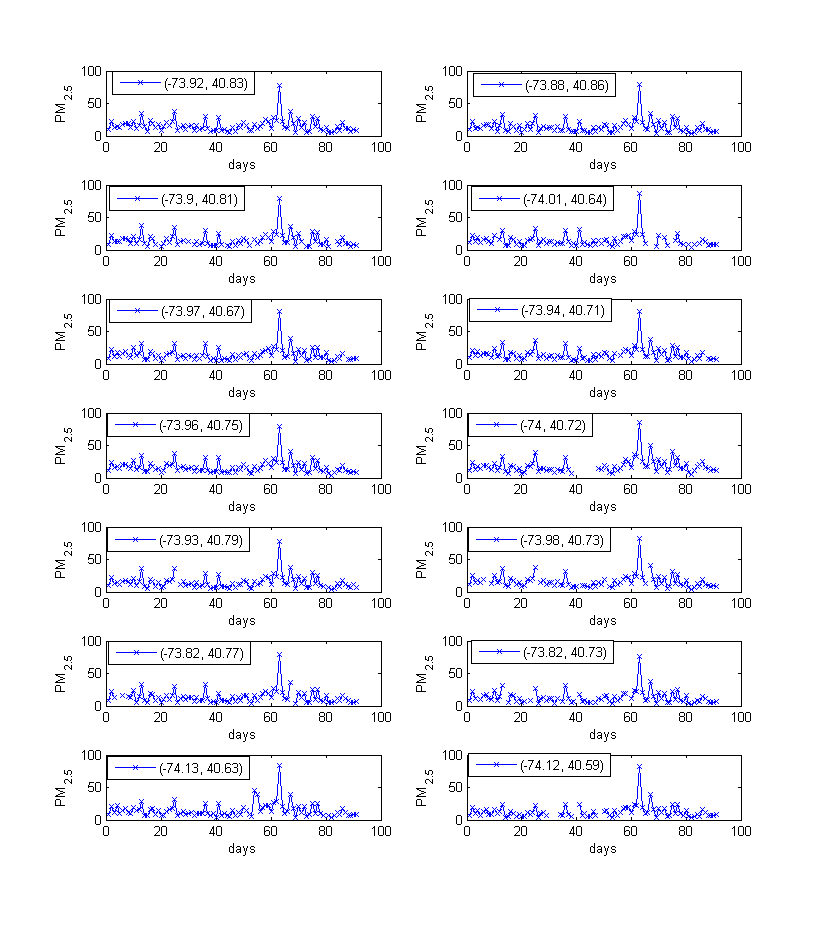
Figure 1: Time Series Data at the 14 locations with their spatial coordinates

Out of $1365$ data points, $126$ were missing  and the missing values are estimated as follows. Let $X\left(\mathbf{s}_{i},t\right)$  $(i=1,\ 2,\ \ldots 15;$ $t=1,\ 2,\ \ldots 91)$ denote the PM_2.5  observation at the location $\mathbf{s}_{i}$ and at time $t$ and suppose the observation $X\left(\mathbf{s}_{0},t_{0}\right)$ is missing. The missing observation is estimated by averaging over the data at other locations at time $t_{0}$ by $\widetilde{X}\left(\mathbf{s}_{0},t_{0}\right)=(1/14)\sum_{j=1,\neq 0}^{14}X\left(\mathbf{s}_{{}_{j}},t_{0}\right)$.

We used the first differences $\{Y_{t}\left(\mathbf{s}\right)=\Delta_{t}X\left(\mathbf{s},t\right):\mathbf{s}\in\mathbb{R}^{2},\ \ t\in\mathbb{Z\}}$ to remove the linear trend as suggested by [19], and used the detrended data for our analysis. The time series data from the $14$ locations are plotted in Figure 1. The location $11$ (with coordinates: latitude $-73.84$, longitude $40.77$) has large number of missing values (only the first 23 observations are available) and, therefore, we have chosen to estimate all 91 observations at this location using the data from other 14 locations. We compared the estimated values with the 23 observed . The sample auto-correlation plots of the $14$ series have shown strong correlation at lag $1$. On the basis of BIC criterion, we decided that the $14$ time series can adequately be modelled by an AR(1) model. The corresponding second order spectrum is   $g_{0}\left(\omega,\vartheta\right)=\sigma^{2}{\large/}\left|1+\varphi z\right|^{2}$ where $z=\exp(i\omega)$ and the vector of the parameters   are$\ \vartheta$ $=(\sigma^{2},\phi)$  and these are estimated  by minimizing the criterion (26) with $L=91$. We note that we scaled the equation (7) such that $\sigma_{e}^{2}=\sigma^{2}$, see (14).

The final estimates  of the AR model have been found to be $\widehat{\varphi}=0.4659$;  $\widehat{\sigma}=5.9264$. Using these estimated values, all the elements of the vector $G_{0}\left(\omega\right)$ and the elements of   the square matrix $F_{m}\left(\omega\right)$ (which is of order $14\times 14$) are evaluated. The vectors $J_{0}(\omega)$ at the  Fourier frequencies  $\omega_{k}=2\pi k/2^{6}$ are estimated using the equation $\underline{\widehat{G}}_{0}^{\prime}\left(\omega_{k}\right)\widehat{F}_{m}^{-1}\left(\omega_{k}\right)\underline{J}_{m}\left(\omega_{k}\right)$. The data at the location $11$ are estimated using the equation (17). The plot of the 91 estimated values (with (+) sign), plot of the first $23$ given observations (with $o$ sign), corresponding $95\%$ confidence bands using (27) are given in Fig 2. We see a good agreement between the estimated values and the observed values, suggesting that  the prediction methodology works very well in this case. Also we find that the strong spatial correlation and the temporal correlation  can satisfactorily be described by the spatio-temporal covariance function  defined here.

Figure 2: Location 11. Plot of the observed values (denoted by + sign), predicted values (denoted by ’o’ sign), 95% prediction intervals (denoted by – sign)

In order to check  the overall performance, we computed the leave-one-out cross-validation ([9]) criterion . Here we estimated the data at one location, taken one at a time, using the data given at other 13 locations. The Mean Square Error calculated for all the 14 locations is

$$MSSE=\sum SSE\left(j\right)/(14\ast 91)=15.3050,$$

where

$$SSE\left(j\right)=\sum_{t=1}^{91}\left(Y_{t}\left(\mathbf{s}_{j}\right)-\widehat{Y}_{t}\left(\mathbf{s}_{j}|\mathbf{s}_{k}\neq\mathbf{s}_{j}\right)\right)^{2},$$

and $\widehat{Y}_{t}\left(\mathbf{s}_{j}|\mathbf{s}_{k}\neq\mathbf{s}_{j}\right)$ is the estimator of the data at time $t$ at location $\mathbf{s}_{j}$ conditional on the data at the locations $\left\{\mathbf{s}_{1},\mathbf{s}_{2},\ldots\mathbf{s}_{j-1},\mathbf{s}_{j+1},\ldots\mathbf{s}_{13}\right\}$. We have also estimated the prediction error variance using the equation (21)  for each location, and they are shown in Fig 3 (the larger the diameter of the circle, the higher the variance).

We estimated the PM_2.5 values for all $t=1,2,\ldots 91$ and for all the $625$ locations (including $14$ locations where the data is available). The plot of the these predicted values are given in Fig 4..

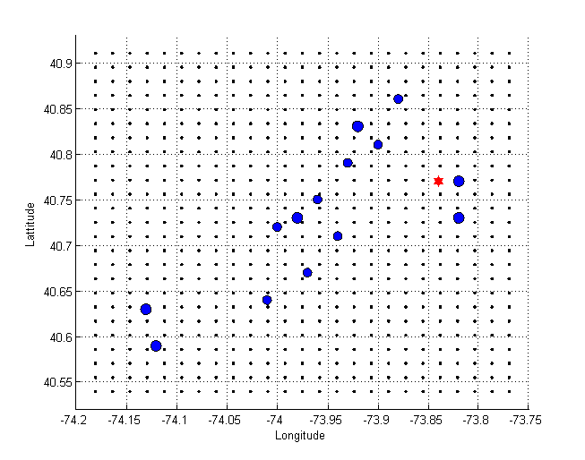
Figure 3: Grid of the 625 locations. Dark circles correspond to the locations (data available).

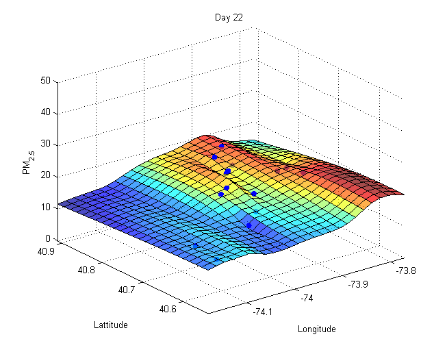
Figure 4: Estimated PM_2.5 for all the locations at $t=22$.

To check the forecasting performance of the method described  here we considered the prediction at the location #8. We considered the data, $t=1,2,...83$ as given and estimated the rest of the values ($84,83,\ldots 91$) using the AR(1) model fitted. The forecasting methodology is well known, and therefore, we briefly summarise the method (details can be found in any time series book).

Let

$$\widehat{Y}_{n+h}\left(\mathbf{s}_{0}|t=1,2,\ldots,n;\mathbf{s}_{j};j=1,2,\ldots m\right)=E\left(Y_{n+h}\left(\mathbf{s}_{0}\right)|Y_{t}\left(\mathbf{s}_{j}\right);t=1,2,\ldots n,\mathbf{s}_{j};j=1,2,\ldots m\right)\ \$$

For the AR(1) model fitted, we have

$$\widehat{Y}_{n+h}\left(\mathbf{s}_{0}|t=1,2,\ldots n,\mathbf{s}_{j};j=1,2,\ldots m\right)=\varphi^{h}\widehat{Y}_{n}\left(\mathbf{s}_{0}\right),$$

hence

$$Y_{n+h}\left(\mathbf{s}_{0}\right)-\widehat{Y}_{n+h}\left(\mathbf{s}_{0}\right)=\varphi^{h}\left(Y_{n+h}\left(\mathbf{s}_{0}\right)-\widehat{Y}_{n}\left(\mathbf{s}_{0}\right)\right)+\sum_{k=1}^{h}\varphi^{k-1}\varepsilon_{n+k}\left(\mathbf{s}_{0}\right),$$

where $\widehat{Y}_{n}\left(\mathbf{s}_{0}\right)$ denotes the spatial prediction and $\varepsilon_{t}\left(\mathbf{s}_{0}\right)$ is the innovation error at $\mathbf{s}_{0}$ and at time $t$. Therefore, we obtain

$$E\left(Y_{n+h}\left(\mathbf{s}_{0}\right)-\widehat{Y}_{n+h}\left(\mathbf{s}_{0}\right)\right)^{2} =\varphi^{2h}E\left(Y_{n}\left(\mathbf{s}_{0}\right)-\widehat{Y}_{n}\left(\mathbf{s}_{0}\right)\right)^{2}+\sigma^{2}\frac{\varphi^{2h}-1}{\varphi^{2}-1}$$

$$=\varphi^{2h}\int\limits_{-\pi}^{\pi}\sigma_{m}^{2}\left(\omega\right)d\omega+\sigma^{2}\frac{\varphi^{2h}-1}{\varphi^{2}-1}.$$ (27)

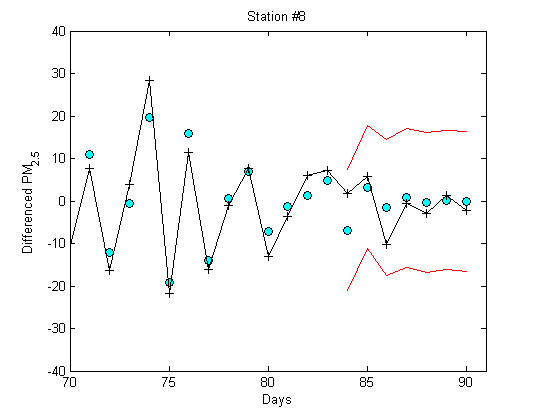
Figure 5: Location 8. Predicted values (’o’). observed values (+), Prediction intervals (–)

7 Appendix: Discrete Fourier Transforms and their properties

Let us assume that we have time series data from $m$ locations spatially distributed.
Let $\left\{Y_{t}\left(\mathbf{s}_{i}\right)|i=1,2,\ldots m;\ t=1,\ldots,n\right\}$, be a sample from the zero mean spatio-temporal stationary process $\left\{Y_{t}\left(\mathbf{s}\right)\right\}$.  Consider the time series data $\left\{Y_{t}\left(\mathbf{s}_{i}\right)|t=1,\ldots,n\right\}$ at the location $\mathbf{s}_{i}$, and define the Discrete Fourier transform (DFT)

$$J_{\mathbf{s}_{i}}\left(\omega_{k}\right)=\frac{1}{\sqrt{2\pi n}}\sum\limits_{t=1}^{n}Y_{t}\left(\mathbf{s}_{i}\right)e^{-it\omega_{k}},$$ (28)

where $\omega_{k}=\frac{2\pi k}{n},\ \ k=0,\ \pm 1,\ \ldots,\ \pm\left[\frac{n}{2}\right]$. In practice one uses Fast Fourier Transform algorithm to compute the DFT.  It is well known that the number of operations required to calculate $n$ discrete Fourier transforms from $n$ dimensional data is of order $\ n\log n$. The corresponding second order periodogram  is defined as

$$I_{\mathbf{s}_{i}}\left(\omega_{k}\right)=\left|J_{\mathbf{s}_{i}}\left(\omega_{k}\right)\right|^{2},$$

and the cross periodogram between the time series $\left\{Y_{t}\left(\mathbf{s}_{i}\right)\right\}$  and $\left\{Y_{t}\left(\mathbf{s}_{j}\right)\right\}$ is given by $I_{\mathbf{s}_{i}s_{j}}\left(\omega_{k}\right)=J_{\mathbf{s}_{i}}\left(\omega_{k}\right)J_{\mathbf{s}_{j}}^{\ast}\left(\omega_{k}\right)$.

It is well known that the periodogram  is an asymptotically unbiased estimator of the second order spectral density function, but it is not mean square consistent and hence  to obtain a consistent estimate the periodograms are smoothed using various kernels (see [17]). It is well known  that (see  for example [17])

$$E\left(J_{\mathbf{s}_{i}}\left(\omega\right)\right) =0,$$

$$Var\left(J_{\mathbf{s}_{i}}\left(\omega\right)\right) =E\left(I_{\mathbf{s}_{i}}\left(\omega\right)\right)\simeq g_{\mathbf{s}_{i}}\left(\omega\right)=g_{0}(\omega),$$ (29)

where $g_{0}(\omega)$ is the second order spectral density function of the random process. We further note that $\sigma_{Y}^{2}=\int g_{0}(\omega)d\omega$. From (28), by inversion we get

$$Y_{t}\left(\mathbf{s}\right)=\sqrt{\frac{n}{2\pi}}\int\limits_{-\pi}^{\pi}J_{\mathbf{s}}\left(\omega\right)e^{it\omega}d\omega\text{.}$$ (30)

The above relation (given by the (30)) shows that the process $Y_{t}\left(\mathbf{s}\right)$ can be decomposed into sine and cosine functions, and the amplitude $J_{\mathbf{s}}\left(\omega\right)$ measures the contribution made by the harmonic component with frequency $\omega$ to the estimated total power $\sigma_{Y}^{2}$. It  is also well known that the power spectrum $g_{0}(\omega)$  is a frequency decomposition of the power $\sigma_{Y}^{2}$ of the signal  $\{Y_{t}\left(\mathbf{s}_{i}\right)\}$ and, therefore, performing spectral analysis on the data is considered to be equivalent to the classical analysis of variance (ANOVA), where one checks for the contribution of each component in the regression model via ANOVA decomposition.

In the following proposition we summarise the well known properties of the Fourier Transforms of stationary process. For details refer to [2], [17], [8].

Proposition 1

Let $J_{\mathbf{s}_{i}}\left(\omega_{k}\right)$ and $J_{\mathbf{s}_{j}}\left(\omega_{k}\right)$ be the discrete Fourier Transforms of the spatio-temporal stationary processes $\{Y_{t}\left(\mathbf{s}_{i}\right)\},\ \{Y_{t}\left(\mathbf{s}_{j}\right)\}$ respectively. For large $n$,

$$Cov\left(J_{\mathbf{s}_{i}}\left(\omega_{k}\right),J_{\mathbf{s}_{i}}\left(\omega_{k^{{}^{\prime}}}\right)\right)\simeq 0,\quad k\neq k^{\prime},$$

$$Cov\left(J_{\mathbf{s}_{i}}\left(\omega_{k}\right),J_{\mathbf{s}_{j}}\left(\omega_{k}\right)\right) =E\left[I_{\mathbf{s}_{i}\mathbf{s}_{j}}\left(\omega_{k}\right)\right]$$

$$\simeq\frac{1}{2\pi}\sum\limits_{n=-\infty}^{\infty}c\left(\mathbf{s}_{i}-\mathbf{s}_{j},n\right)e^{-in\omega_{k}}=g_{\mathbf{s}_{i}-\mathbf{s}_{j}}\left(\omega_{k}\right),$$ (31)

where $g_{\left(\mathbf{s}_{i}-\mathbf{s}_{j}\right)}\left(\omega\right)$ is defined as the cross spectrum between the two processes and it is usually a complex valued function. If the process is isotropic, then

$$c\left(\mathbf{s}_{i}-\mathbf{s}_{j},n\right)=c\left(\left\|\mathbf{s}_{i}-\mathbf{s}_{j}\right\|,n\right)=c\left(\left\|\mathbf{s}_{i}-\mathbf{s}_{j}\right\|,-n\right)\text{.}$$

and under the isotropy assumption the cross spectrum $g_{\mathbf{s}_{i}-\mathbf{s}_{j}}\left(\omega\right)$ between the two processes reduces to

$$g_{\parallel\mathbf{h}\parallel}(\omega)=\frac{1}{2\pi}\sum\limits_{n=-\infty}^{\infty}c(\left\|\mathbf{h}\right\|,n)e^{-in\omega},\quad\left|\omega\right|\leq\pi,$$

and the spectral function $g_{\parallel\mathbf{h}\parallel}(\omega)$, where $\ \left\|\mathbf{h}\right\|=\left\|\mathbf{s}_{i}-\mathbf{s}_{j}\right\|,\$is  real and symmetric in $\omega$.

Proof. The above results are well known and hence details are omitted.   

If the random process $\left\{Y_{t}\left(\mathbf{s}_{i}\right)\right\}$ is Gaussian, then the complex valued random variables
$\left\{J_{\mathbf{s}_{i}}\left(\omega_{k}\right)|\ k=0,1,\ldots,\left[\frac{n}{2}\right]\right\}$ will be asymptotically independent,  and will be distributed as complex Gaussian,  and each $J_{\mathbf{s}_{i}}\left(\omega_{k}\right)$ will be distributed as complex normal with mean zero and variance proportional to $g_{0}\left(\omega_{k}\right)$.

As pointed out earlier the second order periodogram $\ I_{\mathbf{s}_{i}}(\omega)$ defined above is always real, whereas the cross periodogram $I_{\mathbf{s}_{i},\mathbf{s}_{j}}\left(\omega_{k}\right)$ defined above between the spatial processes $\left\{Y_{t}\left(\mathbf{s}_{i}\right)\right\}$ and $\left\{Y_{t}\left(\mathbf{s}_{j}\right)\right\}$  is usually a complex valued function. Under the isotropy assumption, however, the cross spectrum is a  function of the Euclidean distance $\ \left\|\mathbf{h}\right\|=\left\|\mathbf{s}_{i}-\mathbf{s}_{j}\right\|$ and the temporal frequency $\omega$ (i.e., spectral in time, but not in space) and, therefore, it is real. It is interesting to see the similarity between the above function   and the spectral density functions defined by [5] and [23] which are spectral in time but not in space.

In the following proposition we show that the Discrete Fourier Transform  of $Y_{t}\left(\mathbf{s}\right)$ can be written in terms of  orthogonal set function $Z_{Y}\left(\underline{\lambda},\omega\right)$.

Proposition 2

Let $\ J_{\mathbf{s}}\left(\omega\right)$ be the Discrete Fourier Transform of $\{Y_{t}(s)\}$ and let the spectral representation of $Y_{t}(s)$ be given by (3). Then

$$J_{\mathbf{s}}\left(\omega\right)\simeq\int e^{i\underline{s}\,\underline{\lambda}}\sqrt{\frac{n}{2\pi}}dZ_{Y}\left(\underline{\lambda},\omega\right).$$ (32)

Proof. Substitute the spectral representation (3) for $Y_{t}\left(\mathbf{s}\right)$ in (28), and after some simplification, we obtain

$$J_{\mathbf{s}}\left(\omega\right)=\int\int e^{i\underline{s}\,\underline{\lambda}}\left[e^{i\left(n+1\right)\frac{\varphi}{2}}F_{n}^{\frac{1}{2}}\left(\varphi\right)\right]dZ_{Y}\left(\underline{\lambda},\omega\right),$$ (33)

where $\varphi=\mu-\omega$, $\int$ is a $d$ dimensional multiple integral, (see [17], p. 419) and in obtaining the above, we used the result

$$\sum\limits_{t=1}^{n}e^{it\varphi}=e^{i\left(n+1\right)\frac{\varphi}{2}}\left[\frac{\sin n\frac{\varphi}{2}}{\sin\frac{\varphi}{2}}\right]=e^{i\left(n+1\right)\frac{\varphi}{2}}\sqrt{2\pi n}F_{n}^{\frac{1}{2}}\left(\varphi\right)\text{, }$$

where the Fejér kernel $F_{n}\left(\varphi\right)$ is given by

$$F_{n}\left(\varphi\right)=\frac{1}{2\pi n}\frac{\sin^{2}n\frac{\varphi}{2}}{\sin^{2}\frac{\varphi}{2}}\text{.}$$

It is well known that the Fejér kernel behaves like a Dirac Delta function as $n\rightarrow\infty$ and as $\varphi\rightarrow 0$, $F_{n}\left(\varphi\right)=\mathit{O}\left(n\right)$. As pointed out by [17], p. 419), that $F_{n}^{\frac{1}{2}}\left(\varphi\right)$ does not strictly tend to a Dirac Delta $\delta-$function as $n\rightarrow\infty$, nevertheless, behaves in a similar manner to a $\delta-$function. In particular as $n\rightarrow\infty$ and for all $\varphi\neq 0$, $F_{n}^{\frac{1}{2}}\left(\varphi\right)\rightarrow 0$, and as $\varphi\rightarrow 0$, $F_{n}^{\frac{1}{2}}\left(\varphi\right)\rightarrow\sqrt{n/2\pi}$. Therefore, as $n\rightarrow\infty$, $F_{n}^{\frac{1}{2}}\left(\varphi\right)$ vanishes everywhere except at the origin. In view of this, for large $n$, we  have the result

$$J_{\mathbf{s}}\left(\omega\right)\simeq\int e^{i\underline{s}\,\underline{\lambda}}\sqrt{\frac{n}{2\pi}}dZ_{Y}\left(\underline{\lambda},\omega\right).$$

We note that the above integral is over the wave number space $\lambda$ only.   

Proposition 3

Let $\left\{e_{t}(\mathbf{s)}|\mathbf{s}\in\mathbb{R}^{d},t\in\mathbb{Z}\right\}$ be a white noise process in space and time, that is, we assume the process has constant spectrum, it satisfies the following conditions.

$$E\left(e_{t}\left(\mathbf{s)}\right)\right) =0,$$

$$Var(e_{t}\left(\mathbf{s)}\right) =\sigma_{e}^{2}\text{, does not depend on }\mathbf{s}\text{ or }t,$$

$$Cov\left(e_{t}\left(\mathbf{s)}\right),e_{t^{{}^{\prime}}}\left(\mathbf{s)}\right)\right) =\sigma_{e}^{2}I\left(\mathbf{s},\mathbf{s}^{\prime}\right)I\left(t,t^{\prime}\right),$$

where

$$I(\mathbf{s},\mathbf{s}^{\prime}) =\left\{\begin{array}[c]{c}1\text{ if }\mathbf{s}=\mathbf{s}^{\prime},\\ 0\text{ otherwise, }\end{array}\right.$$

$$I(t,t^{\prime}) =\left\{\begin{array}[c]{c}1\text{ if }t=t^{\prime},\\ 0\text{ otherwise.}\end{array}\right.$$

Let the Discrete Fourier transform of the white noise process be

$$J_{\mathbf{s},e}\left(\omega\right)=\frac{1}{\sqrt{2\pi n}}\sum\limits_{t=1}^{n}e_{t}(\mathbf{s)}e^{-it\omega}.$$

Then

$$J_{\mathbf{s},e}\left(\omega\right)\simeq\int e^{i\mathbf{s}\cdot\underline{\lambda}}\left[\sqrt{\frac{n}{2\pi}}\right]dZ_{e}\left(\underline{\lambda},\omega\right),$$ (34)

where the orthogonal random process $Z_{e}\left(\underline{\lambda},\omega\right)$ satisfies

$$EdZ_{e}\left(\underline{\lambda},\omega\right) =0,$$

$$E\left|dZ_{e}\left(\underline{\lambda},\omega\right)\right|^{2} =\frac{\sigma_{e}^{2}}{\left(2\pi\right)^{d+1}}d\underline{\lambda}d\omega\text{.}$$

Proof. It is similar to Proposition 2 and hence omitted.   

Acknowledgement. The publication was supported by the TÁMOP-4.2.2.C-11/1/KONV-2012-0001 project. The project has been supported by the European Union, co-financed by the European Social Fund. The visit of Subba Rao to the CRRAO AIMSCS was supported by a grant from the Department of Science and Technology, Government of India, grant number SR/S4/516/07. The authors are thankful to the editor, co-editor and the referees for their valuable comments and suggestions. They are also thankful to Dr Suhasini Subba Rao, Texas A&M University,  USA for her suggestions for improvement of the paper.

References

- [1] M. Abramowitz and I. A. Stegun. Handbook of mathematical functions with formulas, graphs, and mathematical tables. Dover Publications Inc., New York, 1992. Reprint of the 1972 edition.
- [2] D. R. Brillinger. Time Series; Data Analysis and Theory. Society for Industrial and Applied Mathematics (SIAM), Philadelphia, PA, 2001. Reprint of the 1981 edition.
- [3] P. F. Craigmile and P. Guttorp. Space-time modelling of trends in temperature series. Journal of Time Series Analysis, 32(4):378–395, 2011.
- [4] N. Cressie. Statistics for Spatial Data. Wiley Series in Probability & Mathematical Statistics, 1993.
- [5] N. Cressie and H.-C. Huang. Classes of nonseparable, spatio-temporal stationary covariance functions. Journal of the American Statistical Association, 94(448):1330–1339, 1999.
- [6] N. Cressie and C. K. Wikle. Statistics for Spatio-Temporal Data. Wiley Series in Probability and Statistics, 2011.
- [7] P. J. Diggle and P. J. Ribeiro. Model-based geostatistics. Springer, 2007.
- [8] Y. Dwivedi and S. Subba Rao. A test for second-order stationarity of a time series based on the discrete fourier transform. Journal of Time Series Analysis, 32(1):68–91, 2011.
- [9] R. Giraldo, P. Delicado, and J. Mateu. Continuous time-varying kriging for spatial prediction of functional data: An environmental application. Journal of agricultural, biological, and environmental statistics, 15(1):66–82, 2010.
- [10] T. Gneiting. Nonseparable, stationary covariance functions for space–time data. Journal of the American Statistical Association, 97(458):590–600, 2002.
- [11] R. H. Jones and Y. Zhang. Models for continuous stationary space-time processes. In Modelling longitudinal and spatially correlated data, pages 289–298. Springer, 1997.
- [12] F. Lindgren, H. Rue, and J. Lindström. An explicit link between gaussian fields and gaussian markov random fields: the stochastic partial differential equation approach. Journal of the Royal Statistical Society: Series B (Statistical Methodology), 73(4):423–498, 2011.
- [13] C. Ma. Spatio-temporal covariance functions generated by mixtures. Mathematical geology, 34(8):965–975, 2002.
- [14] C. Ma. Spatio-temporal stationary covariance models. Journal of Multivariate Analysis, 86(1):97–107, 2003.
- [15] H. Ombao, X. Shao, E. Rykhlevskaia, M. Fabiani, and G. Gratton. Spatio-spectral analysis of brain signals. Statistica Sinica, 18(4):1465, 2008.
- [16] M. B. Priestley. Evolutionary spectra and non-stationary processes. Journal of the Royal Statistical Society. Series B (Methodological), pages 204–237, 1965.
- [17] M. B. Priestley. Spectral Analysis and Time Series. Academic Press, New York, 1981.
- [18] M. D. Ruiz-Medina. New challenges in spatial and spatiotemporal functional statistics for high-dimensional data. Spatial Statistics, 1:82–91, 2012.
- [19] S. K. Sahu and K. V. Mardia. A bayesian kriged kalman model for short-term forecasting of air pollution levels. Journal of the Royal Statistical Society: Series C (Applied Statistics), 54(1):223–244, 2005.
- [20] F. Sigrist, H. R Künsch, and W. A Stahel. Stochastic partial differential equation based modelling of large space–time data sets. Journal of the Royal Statistical Society: Series B (Statistical Methodology), 77(1):3–33, 2015.
- [21] E. M. Stein and G. Weiss. Introduction to Fourier analysis on Euclidean spaces. Princeton University Press, Princeton, N.J., 1971. Princeton Mathematical Series, No. 32.
- [22] M. L. Stein. Interpolation of spatial data: some theory for kriging. Springer, 1999.
- [23] M. L. Stein. Space–time covariance functions. Journal of the American Statistical Association, 100(469):310–321, 2005.
- [24] M. L. Stein. Statistical methods for regular monitoring data. Journal of the Royal Statistical Society: Series B (Statistical Methodology), 67(5):667–687, 2005.
- [25] M. L. Stein, Z. Chi, and L. J. Welty. Approximating likelihoods for large spatial data sets. Journal of the Royal Statistical Society: Series B (Statistical Methodology), 66(2):275–296, 2004.
- [26] T. Subba Rao, S. Das, and G. Boshnakov. A frequency domain approach for the estimation of parameters of spatio-temporal random processes. Journal of Time Series Analysis, 35:357–377, 2014.
- [27] T. Subba Rao and Gy. Terdik. Statistical analysis of spatio-temporal models and their applications. In T. Subba Rao, S. Subba Rao, and C. R.. Rao, editors, Handbook of statistics: time series analysis: methods and applications, volume 30, chapter 18, pages 521–540. Elsevier, 2012.
- [28] A. V. Vecchia. Estimation and model identification for continuous spatial processes. Journal of the Royal Statistical Society. Series B (Methodological), 50:297–312, 1988.
- [29] P. Whittle. On stationary processes in the plane. Biometrika, 41(3/4):434–449, 1954.