Orbital magnetization of insulating perovskite transition-metal oxides with the net ferromagnetic moment in the ground state

Abstract

Modern theory of the orbital magnetization is applied to the series of insulating perovskite transition metal oxides (orthorhombic YTiO₃, LaMnO₃, and YVO₃, as well as monoclinic YVO₃), carrying a net ferromagnetic (FM) moment in the ground state. For these purposes, we use an effective Hubbard-type model, derived from the first-principles electronic-structure calculations and describing the behavior of magnetically active states near the Fermi level. The solution of this model in the mean-field Hartree-Fock approximation with the relativistic spin-orbit coupling typically gives us a distribution of the local orbital magnetic moments, which are related to the site-diagonal part of the density matrix $\hat{\cal D}$ by the “standard” expression $\boldsymbol{\mu}^{0}=-\mu_{\rm B}\mathrm{Tr}\{\hat{\textbf{L}}\hat{\cal D}\}$ and which are usually well quenched by the crystal field. In this work, we evaluate “itinerant” corrections $\Delta\boldsymbol{\cal M}$ to the net FM moment, suggested by the modern theory. We show that these corrections are small and in most cases can be neglected. Nevertheless, the most interesting aspect of our analysis is that, even for these compounds, which are typically regarded as normal Mott insulators, the “itinerant” corrections reveal a strong k-dependence in the reciprocal space, following the behavior of Chern invariants. Therefore, the small value of $\Delta\boldsymbol{\cal M}$ is the result of strong cancelation of relatively large contributions, coming from different parts of the Brillouin zone. We discuss details as well as possible implications of this cancelation, which depends on the crystal structure as well as the type of the magnetic ground state.

I Introduction

Orbital magnetism is one of the oldest and most fundamental phenomena. All our present understanding of magnetism developed from the classical concept of orbital motion, which is much older than the concept of spin. The orbital magnetization can be probed by many experimental techniques, including susceptibility measurement, electron paramagnetic resonances, x-ray magnetic circular dichroism, neutron diffraction, etc.White ; Syncrotron ; Lander

At the same time, the orbital magnetism appears to be one of the most difficult and challenging problems for the theory, especially when it comes to the level of first-principles electronic structure calculations. If the methods of spin magnetism are relatively well elaborated, the study of orbital magnetism is sometimes regarded to be on a primitive stage. There are two reasons for it.

The first one is that the spin magnetism, in principle, allows for the description starting from the limit of homogeneous electron gas, which is widely used as an approximation for the exchange-correlation energy (the so-called local spin density approximation or LSDA) in the spin-density functional theory (SDFT). On the contrary, the orbital magnetism implies some inhomogeneities of the medium, being associated with either the spin-orbit (SO) interaction or the external vector potential, which are necessary to induce the magnetization.remark2 Therefore, for the correct description of orbital magnetization on the level of first-principles electronic structure calculations, it is essential to go beyond the homogeneous electron gas limit. Furthermore, there may be even more fundamental problem, related to the fact that the Kohn-Sham SDFT (even the exact one) does not necessary guarantee to yield correct orbital currents and, therefore, the orbital magnetization, which is defined in terms of these currents.VignaleRasolt This means that the orbital magnetization (or any related to it quantity) should be treated as an independent variational degree of freedom in the density functional theory (DFT).Jansen Historically, this problem in calculations of the orbital magnetization was noticed first, and on earlier stages all the efforts were mainly concentrated on the improvement of SDFT, by introducing different kinds of semi-empirical orbital functionals (Refs. OPB, ; Norman, ; LDAU, ; Minar, ) or moving in the direction of ab initio current SDFT (Ref. Ebert, ). Most of these theories emphasized the local character of the orbital magnetization, implying that (i) it can be computed using the standard expression

$$\boldsymbol{\mu}^{0}=-\mu_{\rm B}\mathrm{Tr}\{\hat{\textbf{L}}\hat{\cal D}\}$$ (1)

for the expectation value of the angular momentum operator $\hat{\textbf{L}}$ in terms of the site-diagonal part of the density matrix $\hat{\cal D}$, where $\mu_{\rm B}=e\hbar/2mc$ is the Bohr magneton in terms of the electron charge ($-$$e$), its mass ($m$), the Plank constant ($\hbar$), and the velocity of light ($c$); and (ii) the effect of exchange-correlation interactions on $\boldsymbol{\mu}^{0}$ can be also treated in the local form, by considering only properly screened on-site interactions and the same site-diagonal elements of the density matrix (Ref. OPB, ; Norman, ; LDAU, ) or of the lattice Green function (Ref. Minar, ). Even today, the problem of how to “decorate” DFT in order to describe properly the effects of orbital magnetism in solids is largely unresolved and continues to be one of the most important and interesting issues.

Nevertheless, the new turn in the theory of orbital magnetism was not directly related to fundamentals of DFT. It was initiated by another fundamental question of how the orbital magnetization should be computed for extended periodic systems. This new direction, which we will refer to as the “modern theory of orbital magnetization”, emerged nearly one decade ago and is a logical continuation of the similar theory of electric polarization:KSV ; Resta as the position operator r is not well defined in the Bloch representation, similar problem is anticipated for the orbital magnetization operator $(-e/2c)\textbf{r}\times\textbf{v}$, which is also expressed through r. Then, the correct consideration of thermodynamic limit yielded a new and rather nontrivial expression for the orbital magnetization, being another interesting manifestation of the Berry-phase physics.Resta ; XiaoPRL ; ThonhauserPRL ; CeresoliPRB ; ShiPRL ; ThonhauserIJMPB

The modern theory of the orbital magnetization is basically an one-electron theory. It does not say anything about the form of exchange-correlation interactions. Therefore, it would not be right to think that applications of the modern theory will automatically resolve all previous problems, related to the form of the exchange-correlation functional and limitations of LSDA.

Practical implementations of the modern theory of orbital magnetization are still rather limited. Moreover, many of them are devoted to rather exotic Haldane model Hamiltonian,Haldane which is typically used in order to illustrate the basic ideas (Refs. ThonhauserPRL, ; CeresoliPRB, ) and to test computational schemes (Ref. CeresoliResta, ). The first-principles calculations were performed only for ferromagnetic metals Fe, Co, and Ni, where the modern theory slightly improves the values of orbital magnetization in comparison with the experimental data,ThonhauserIJMPB ; fp3d and the orbital magnetoelectric coupling in insulators.mecoupling

At the same time, several important aspects of the modern theory remain obscure. To begin with, even if the previous treatment of the orbital magnetization was incomplete, it is not immediately clear what was missing in the “standard” expression (1) and whether it can still be used in practical calculations for real materials. Then, what is the meaning of the new corrections to Eq. (1), suggested by the modern theory?

In this work, we apply the modern theory of the orbital magnetization to the series of representative distorted perovskite transition-metal oxides with the net ferromagnetic (FM) moment in the ground state. Particularly, we consider orthorhombic canted spin ferromagnet YTiO₃, and three weak ferromagnets: orthorhombic LaMnO₃ and YVO₃, as well as monoclinic YVO₃. These compounds differ by the type of the magnetic ground state as well as the microscopic origin of the weak ferromagnetism: regular spin canting caused by Dzyloshinskii-Moriya interactions in orthorhombic systems (Refs. DM, ; Treves, ) versus incomplete compensation of magnetic moments between two crystallographic sublattices in monoclinic YVO₃.review2008 The magnetic structure of these materials depends on a subtle interplay of the crystal distortion, relativistic SO coupling, and electron correlations in the magnetically active bands. Therefore, from the computational point of view, it is more convenient to work with an effective Hubbard-type model, derived from the first-principles electronic structure calculations, and focusing on the behavior of these magnetically active bands.review2008 The previous applications showed that such a strategy is very promising and the effective model provides a reliable description for magnetic ground-state properties of YTiO₃, YVO₃, and LaMnO₃.review2008 ; JPSJ ; t2g

The rest of the paper is organized as follows. In Sec. II we briefly remind to the reader the main aspects of the modern theory of the orbital magnetization in solids. In Sec. III, we identify the main contributions to the net orbital magnetic moment in the case of basis – when the Bloch wavefunction is expanded over localized Wannier-type orbitals, centered at magnetic sites. Then, if the magnetic sites are located in the centers of inversion (the case that we consider), the net orbital magnetic moment will have two contributions: the local one, which is given by the “standard” expression (1), and an “itinerant” correction to it, suggested by the modern theory. The behavior of the second part is closely related to that of Chern invariant, which for the normal insulators with the canted FM structure can be viewed as a “totally itinerant quantity”: the Chern invariant is given by certain Brilloin zone (BZ) integral. The individual contributions to this integral in each k can be finite. However, the total integral, which can be regarded as a local (or site-diagonal) component of some k-dependent property, is identically equal to zero. Then, in Sec. IV we will briefly explain details of our calculations and in Sec. V we will present numerical results for YTiO₃, YVO₃, and LaMnO₃. We will show that the “itinerant” correction to the net orbital magnetic moment is small. However, this small value is a result of cancelation of relatively large contributions, coming from different parts of the BZ. Finally, in Sec. VI we will summarize our work.

II General Theory

According to the modern theory of the orbital magnetization,ThonhauserPRL ; CeresoliPRB ; ShiPRL the net orbital magnetic moment of a normal periodic insulator satisfies the following expression:

$$\boldsymbol{\cal M}=\frac{e}{2\hbar c}\mathrm{Im}\sum_{n}\int_{BZ}\frac{d\textbf{k}}{\Omega}\langle\partial_{\textbf{k}}u_{n\textbf{k}}|\times(H_{\textbf{k}}+E_{n\textbf{k}})|\partial_{\textbf{k}}u_{n\textbf{k}}\rangle,$$ (2)

where $u_{n\textbf{k}}(\textbf{r})=e^{-i\textbf{k}\textbf{r}}\psi_{n\textbf{k}}(\textbf{r})$ is the cell-periodic eigenstate of the Hamiltonian $H_{\textbf{k}}=e^{-i\textbf{k}\textbf{r}}He^{i\textbf{k}\textbf{r}}$, corresponding to the eigenvalue $E_{n\textbf{k}}$, the summation runs over occupied states, and the integration goes over the first BZ with the volume $\Omega$. Eq. (2) was derived using different theoretical frameworks, including semiclassical dynamics of Bloch electrons,XiaoPRL the Wannier functions technique,ThonhauserPRL ; CeresoliPRB and the perturbation theory in an external magnetic field.ShiPRL It is important that all these methods yield the same expression for $\boldsymbol{\cal M}$.

In the modern theory of the orbital magnetization, the behavior of $\boldsymbol{\cal M}$ is closely related to that of Chern invariants

$$\boldsymbol{\cal C}=-\frac{1}{2\pi}\mathrm{Im}\sum_{n}\int_{BZ}d\textbf{k}\,\langle\partial_{\textbf{k}}u_{n\textbf{k}}|\times|\partial_{\textbf{k}}u_{n\textbf{k}}\rangle,$$ (3)

which was originally introduced to characterize the Hall conductance.Thouless For the normal insulators, $\boldsymbol{\cal C}$ itself vanishes. Nevertheless, the integrand of Eq. (3) (which is also related to the Berry curvature in the multi-band case) can be finite, depending on the symmetry of the crystal and the type of the magnetic ground state. Thus, the finite value of $\boldsymbol{\cal M}$ in normal insulators can be viewed as a result of additional modulation of the Berry curvature by the k-dependent quantities $H_{\textbf{k}}$ and $E_{n\textbf{k}}$.

Furthermore, it is understood that all electron-electron interactions are treated in the spirit of Kohn-Sham DFT, that results in the self-consistent determination of the single-particle Hamiltonian $H$ with the SO interaction. It is important that the orbital magnetization (or related to it orbital currents) should participate as an independent variable of the energy functional, so that $\boldsymbol{\cal M}$ can be found through the expectation value of the angular momentum operator in the basis of occupied Kohn-Sham orbitals $\psi_{n\textbf{k}}(\textbf{r})$ of the Hamiltonian $H$.Jansen Nevertheless, as was explained in the Introduction, the form of this functional is not known. Therefore, in practical calculations, we have to rely on additional approximations. In the present work, we use $H$ obtained in the mean-field Hartree-Fock (HF) approximation for the effective Hubbard-type model, which is derived from the first-principles electronic structure calculations and is aimed to capture the behavior of the magnetically active states near the Fermi level.review2008 This model HF approach can be viewed as a functional of the site-diagonal density matrix in the basis of localized Wannier orbitals, which serve as the basis of the effective low-energy model. Thus, the basic strategy of the present work is the following: (i) The HF method is expected to reproduce the local part of the orbital moment, which is related to the site-diagonal density matrix by Eq. (1);LDAU and (ii) We hope that it can also serve as a good starting point for the analysis of other contributions to $\boldsymbol{\cal M}$. Another possibility is to use current DFT, supplemented with some additional approximations for the exchange-correlation energy.Ebert

The first term in Eq. (2), which is called the “local circulation” $\boldsymbol{\cal M}^{LC}$, is the lattice periodic contribution from the bulk Wannier orbitals, while the second terms (the “itinerant circulation”, $\boldsymbol{\cal M}^{IC}$) arises from the surface of the sample and remains finite in the thermodynamic limit.ThonhauserPRL ; CeresoliPRB In the multi-orbital case, each contribution become gauge invariant (and, therefore, can be treated separately) if one uses the covariant derivatives:CeresoliPRB

$$|\partial_{\textbf{k}}u_{n\textbf{k}}\rangle\rightarrow|\tilde{\partial}_{\textbf{k}}u_{n\textbf{k}}\rangle=\left(1-P_{\textbf{k}}\right)|\partial_{\textbf{k}}u_{n\textbf{k}}\rangle,$$ (4)

where $P_{\textbf{k}}=\sum_{n}|u_{n\textbf{k}}\rangle\langle u_{n\textbf{k}}|$ is the ground-state projector. The total moment $\boldsymbol{\cal M}=\boldsymbol{\cal M}^{LC}+\boldsymbol{\cal M}^{IC}$ is not affected by the transformation (4). Moreover, in this covariant form, the formulation becomes gauge invariant not only for the BZ integrals, but also for their integrants in each k-point of the reciprocal space.CeresoliPRB The same holds for the Chern invariants (3). This allows us to discuss the k-dependence of the net orbital magnetic moments.

III Orbital magnetization and basis

In this section we will consider how the main expression for $\boldsymbol{\cal M}$ [Eq. (2)] can be reformulated in the presence of basis. For these purposes, let us expand $|\psi_{n\textbf{k}}\rangle$ over some basis of localized orbitals $|\phi_{\alpha}(\textbf{r}-\textbf{R})\rangle$, centered at atomic sites R:

$$|\psi_{n\textbf{k}}\rangle=\frac{1}{\sqrt{N}}\sum_{\alpha\textbf{R}}c^{\alpha}_{n\textbf{k}}e^{i\textbf{kR}}|\phi_{\alpha}(\textbf{r}-\textbf{R})\rangle,\\$$ (5)

where $N$ is the number of primitive cells, $\alpha$ is a combination of spin and orbital indices (and, if necessary, the site indices in the primitive cell). The basis itself satisfies the orthonormality condition:

$$\langle\phi_{\alpha^{\prime}}(\textbf{r}-\textbf{R}^{\prime})|\phi_{\alpha}(\textbf{r}-\textbf{R})\rangle=\delta_{\alpha^{\prime}\alpha}\delta_{\textbf{R}^{\prime}\textbf{R}}.$$ (6)

In our case, $\{\phi_{\alpha}(\textbf{r}-\textbf{R})\}$ is the basis of the Wannier functions, used for the construction of the effective low-energy model.review2008 However, it can be viewed in a more general sense: for example, as the basis of nearly orthogonal linear muffin-tin orbitals of the LMTO method,LMTO or any orthonormal atomic-like basis.

The use of the basis set is the general practice in numerical calculations. However, apart from computational issues, the goal of this section is to understand what kind of new contributions is provided by the modern theory of the orbital magnetization [Eq. (2)] in comparison with the standard calculations, which are frequently formulated in the atomic-like basis and based on the simplified expression (1).OPB ; Norman ; LDAU For these purposes, we take the wavefunctions in the form (5) and substitute them in Eq. (2). Then, the k-space gradient of $|u_{n\textbf{k}}\rangle$ will have two contributions:

$$|\partial_{\textbf{k}}u_{n\textbf{k}}\rangle =-\frac{i}{\sqrt{N}}\sum_{\alpha\textbf{R}}(\textbf{r}-\textbf{R})e^{-i\textbf{k}(\textbf{r}-\textbf{R})}c^{\alpha}_{n\textbf{k}}|\phi_{\alpha}(\textbf{r}-\textbf{R})\rangle+$$ (7)

$$+\frac{1}{\sqrt{N}}\sum_{\alpha\textbf{R}}e^{-i\textbf{k}(\textbf{r}-\textbf{R})}\partial_{\textbf{k}}c^{\alpha}_{n\textbf{k}}|\phi_{\alpha}(\textbf{r}-\textbf{R})\rangle=|\partial_{\textbf{k}}u_{n\textbf{k}}\rangle^{\mathrm{I}}+|\partial_{\textbf{k}}u_{n\textbf{k}}\rangle^{\mathrm{II}},$$

and we have to consider four possible contributions to Eq. (2): $\langle\partial_{\textbf{k}}u_{n\textbf{k}}|^{\mathrm{I}}\dots|\partial_{\textbf{k}}u_{n\textbf{k}}\rangle^{\mathrm{I}}$, $\langle\partial_{\textbf{k}}u_{n\textbf{k}}|^{\mathrm{I}}\dots|\partial_{\textbf{k}}u_{n\textbf{k}}\rangle^{\mathrm{II}}$, $\langle\partial_{\textbf{k}}u_{n\textbf{k}}|^{\mathrm{II}}\dots|\partial_{\textbf{k}}u_{n\textbf{k}}\rangle^{\mathrm{I}}$, and $\langle\partial_{\textbf{k}}u_{n\textbf{k}}|^{\mathrm{II}}\dots|\partial_{\textbf{k}}u_{n\textbf{k}}\rangle^{\mathrm{II}}$. Moreover, we assume that all transition-metal sites are located in the inversion centers – the situation, which is indeed realized in perovskites with the $Pbnm$ and $P2_{1}/a$ structure. Then, the Wannier functions $\{\phi_{\alpha}(\textbf{r}-\textbf{R})\}$ will be either even or odd with respect to the inversion centers, and we will have the following property:

$$\langle\phi_{\alpha^{\prime}}(\textbf{r}-\textbf{R}^{\prime})|\textbf{r}|\phi_{\alpha}(\textbf{r}-\textbf{R})\rangle=\textbf{R}\delta_{\alpha^{\prime}\alpha}\delta_{\textbf{R}^{\prime}\textbf{R}}.$$ (8)

In this case, after some tedious but rather straightforward algebra, which is explained in Supplemental Materials,SupM one can obtain the following expressions for the local circulation:

$$\boldsymbol{\cal M}^{LC} =\boldsymbol{\cal M}^{0}+\Delta\boldsymbol{\cal M}^{LC}$$ (9)

$$\equiv-\mu_{\rm B}\sum_{n}\sum_{\alpha\alpha^{\prime}}\int_{BZ}\,\frac{d\textbf{k}}{\Omega}\,c^{\alpha^{\prime}*}_{n\textbf{k}}\textbf{L}_{\textbf{k}}^{\alpha^{\prime}\alpha}c^{\alpha}_{n\textbf{k}}$$

$$+\frac{e}{2\hbar c}\,\mathrm{Im}\sum_{n}\sum_{\alpha\alpha^{\prime}}\int_{BZ}\frac{d\textbf{k}}{\Omega}\,\partial_{\textbf{k}}c^{\alpha^{\prime}*}_{n\textbf{k}}\times H_{\textbf{k}}^{\alpha^{\prime}\alpha}\partial_{\textbf{k}}c^{\alpha}_{n\textbf{k}},$$

and the itinerant circulation:

$$\boldsymbol{\cal M}^{IC} =\frac{e}{2\hbar c}\,\mathrm{Im}\sum_{n}\sum_{\alpha}\int_{BZ}\frac{d\textbf{k}}{\Omega}E_{n\textbf{k}}\,\partial_{\textbf{k}}c^{\alpha*}_{n\textbf{k}}\times\partial_{\textbf{k}}c^{\alpha}_{n\textbf{k}},$$ (10)

where

$$H^{\alpha^{\prime}\alpha}_{\textbf{k}}=\frac{1}{N}\sum\limits_{\textbf{R}\textbf{R}^{\prime}}\,\langle\phi_{\alpha^{\prime}}(\textbf{r}-\textbf{R}^{\prime})|H|\phi_{\alpha}(\textbf{r}-\textbf{R})\rangle\,e^{i\textbf{k}(\textbf{R}-\textbf{R}^{\prime})}$$ (11)

and

$$\textbf{L}_{\textbf{k}}^{\alpha^{\prime}\alpha}=\frac{1}{N}\sum_{\textbf{R}\textbf{R}^{\prime}}\langle\phi_{\alpha^{\prime}}(\textbf{r}-\textbf{R}^{\prime})|(\textbf{r}-\textbf{R}^{\prime})\times\textbf{p}|\phi_{\alpha}(\textbf{r}-\textbf{R})\rangle e^{i\textbf{k}(\textbf{R}-\textbf{R}^{\prime})}$$ (12)

are the Wannier matrix elements of Hamiltonian and periodic part of the angular momentum operator (divided by $\hbar$), respectively. Moreover, Eq. (12) implies that the momentum operator p is related to the velocity $\textbf{v}=(i/\hbar)[H,\textbf{r}]$ in a “nonrelativistic fashion”: $\textbf{p}=m\textbf{v}$.

Thus, the local circulation has two terms. The first one ($\boldsymbol{\cal M}^{0}$) is the standard contribution, that is given by periodic part of the angular momentum operator in the Wannier basis. Due to orthonormality condition (6), the main contributions in Eq. (12) arise from the site-diagonal elements with $\textbf{R}=\textbf{R}^{\prime}$. It can be best seen in the LMTO formulation,LMTO where the tail of the basis function $\phi_{\alpha}(\textbf{r}-\textbf{R})$ near the atomic site $\textbf{R}^{\prime}$ is expanded over energy derivatives of $\{\phi_{\alpha}(\textbf{r}-\textbf{R}^{\prime})\}$. Then, since the function is orthogonal to its energy derivative, all contributions with $\textbf{R}\neq\textbf{R}^{\prime}$ in Eq. (12) will vanish after the radial integration. Therefore, $\textbf{L}_{\textbf{k}}^{\alpha^{\prime}\alpha}$ does not depend on k ($\textbf{L}_{\textbf{k}}^{\alpha^{\prime}\alpha}\equiv\textbf{L}^{\alpha^{\prime}\alpha}$), and $\boldsymbol{\cal M}^{0}$ is given by the standard expression, $\boldsymbol{\cal M}^{0}=-\mu_{\rm B}\mathrm{Tr}_{\alpha}\{\hat{\textbf{L}}\hat{\cal D}\}$ in terms of the density matrix $\hat{\cal D}=[{\cal D}^{\alpha\alpha^{\prime}}]$,

$${\cal D}^{\alpha\alpha^{\prime}}=\sum_{n}\int_{BZ}\,\frac{d\textbf{k}}{\Omega}\,c^{\alpha}_{n\textbf{k}}c^{\alpha^{\prime}*}_{n\textbf{k}},$$

where $\hat{\textbf{L}}\equiv[\textbf{L}^{\alpha^{\prime}\alpha}]$ is the site-diagonal matrix and $\mathrm{Tr}_{\alpha}$ is the trace over $\alpha$. Thus, the remaining term $\Delta\boldsymbol{\cal M}=\Delta\boldsymbol{\cal M}^{LC}+\boldsymbol{\cal M}^{IC}$ can be viewed as a correction to $\boldsymbol{\cal M}^{0}$, suggested by the modern theory of the orbital magnetization. $\Delta\boldsymbol{\cal M}$ has the same structure as Eq. (2), and can be obtained after replacing $|\partial_{\textbf{k}}u_{n\textbf{k}}\rangle$ by the column vector $|\partial_{\textbf{k}}c_{n\textbf{k}}\rangle\equiv[\partial_{\textbf{k}}c^{\alpha}_{n\textbf{k}}]$ and $H_{\textbf{k}}$ by the matrix $\hat{H}_{\textbf{k}}\equiv[H^{\alpha^{\prime}\alpha}_{\textbf{k}}]$ in the Wannier basis. The same holds for the Chern invariants (3), where $|\partial_{\textbf{k}}u_{n\textbf{k}}\rangle$ should be also replaced by $|\partial_{\textbf{k}}c_{n\textbf{k}}\rangle$.

In the following, we will also call $\boldsymbol{\cal M}^{0}$ the net local magnetic moment and $\Delta\boldsymbol{\cal M}$ the itinerant correction to $\boldsymbol{\cal M}^{0}$. This is because, for normal insulators, the Chern invariant itself can be regarded as a totally itinerant quantity: It is given by the BZ integral of the Berry curvature. The Berry curvature itself is k-dependent. However, the local component of it, that is given by the BZ integration, is identically equal to zero. Therefore, it is logical to view $\Delta\boldsymbol{\cal M}$, whose from is similar to $\boldsymbol{\cal C}$, also as an itinerant contribution to the net orbital magnetic moment. Moreover, for the totally localized states, $\hat{H}_{\textbf{k}}$ and $E_{n\textbf{k}}$ will not depend on k. Therefore, in this case $\Delta\boldsymbol{\cal M}$ will vanish, similar to $\boldsymbol{\cal C}$. This is another reason why $\Delta\boldsymbol{\cal M}$ can be associated with the itinerant contribution to the orbital magnetic moment. One can also paraphrase this discussion in the following way: the Berry curvature in the BZ integrals (9)-(10) acts as a “filter”, which separates the local part of the orbital magnetization from the itinerant one.

IV Technical Details

All numerical calculations, reported in this work, have been performed for the effective low-energy model, derived from the first-principles electronic structure calculations. First, we construct the effective Hubbard-type model, describing the behavior of magnetically active $t_{2g}$ bands in the case of YTiO₃ and YVO₃, and all $3d$ bands in the case of LaMnO₃. For these purposes, we specify the basis of Wannier orbitals, spanning the subspace of these bands in the local-density approximation (LDA). Then, the parameters of crystal-field splitting, SO interaction, and transfer integrals of the effective model are given by the matrix elements of the LDA Hamiltonian in the Wannier basis. The parameters of screened Coulomb and exchange interactions are obtained by combining constrained LDA and random-phase approximation (RPA) for the screening.review2008 After the construction, the model was solved in the HF approximation. All details, including the behavior of model parameters and results of HF calculations, can be found in Refs. review2008, ; t2g, ; JPSJ, .

Strictly speaking, if the model Hamiltonian $H$ includes the SO interaction term,

$$H_{\mathrm{SO}}=\frac{\hbar}{4m^{2}c^{2}}\boldsymbol{\sigma}\times\boldsymbol{\nabla}V\cdot\textbf{p},$$ (13)

which originates from Pauli equations and is valid in the second order of $1/c$, the velocity operator $\textbf{v}=(i/\hbar)[H,\boldsymbol{r}]$ will consists of two contributions:

$$\textbf{v}=\frac{\textbf{p}}{m}+\frac{\hbar}{4m^{2}c^{2}}\boldsymbol{\sigma}\times\boldsymbol{\nabla}V.$$ (14)

The theory of orbital magnetization implies that the second term in Eq. (14) can be neglected, that results in the nonrelativistic expression $\textbf{p}=m\textbf{v}$. This can be done because the contribution of the second term of Eq. (14) to the orbital magnetic moment (2) is of the order of $1/c^{3}$, which is formally beyond the accuracy of Pauli equations.

In order to calculate $\tilde{\partial}_{\textbf{k}}c_{n\textbf{k}}$ along the direction $i$ of the BZ, we have used the discretized covariant derivative technique, which is well suited for insulators:CeresoliPRB ; ThonhauserIJMPB

$$\tilde{\partial}_{i}c_{n\textbf{k}}=\frac{1}{2|\textbf{q}|}\left(\tilde{c}_{n\textbf{k}+\textbf{q}}-\tilde{c}_{n\textbf{k}-\textbf{q}}\right),$$ (15)

where q is the vector that connects k with the nearby point in the direction $i$ and $\tilde{c}_{n\textbf{k}+\textbf{q}}$ is the “dual” state, defined in terms of the overlap matrix $(S_{\textbf{k},\textbf{k}+\textbf{q}})_{nn^{\prime}}=\langle c_{n\textbf{k}}|c_{n^{\prime}\textbf{k}+\textbf{q}}\rangle$ as

$$\tilde{c}_{n\textbf{k}+\textbf{q}}=\sum_{n^{\prime}}(S^{-1}_{\textbf{k},\textbf{k}+\textbf{q}})_{n^{\prime}n}c_{n^{\prime}\textbf{k}}.$$ (16)

As for the k-space integration, we have used the grid of about $70$$\times$$70$$\times$$50$ points in the first BZ, which guarantees an excellent convergence for $\Delta\boldsymbol{\cal M}$ depending on the number of k-points.SupM

V Results

V.1 YTiO₃

YTiO₃ crystallizes in the orthorhombic $Pbnm$ structure (in our calculations, we used the experimental structure parameters, measured at 2 K).YTiO3exp Below $T_{\rm C}\approx$ 29 K, it forms the canted FM structure, where the net FM moment is parallel to the orthorhombic $\boldsymbol{c}$ axis. Two other components of the magnetic moments, parallel to the orthorhombic $\boldsymbol{a}$ and $\boldsymbol{b}$ axes, are ordered antiferromagnetically. The type of this ordering is G and A, respectively. Such magnetic structure can be abbreviated as G_a-A_b-F_c. It was successfully reproduced by our mean-field HF approximation for the low-energy model. The details of these calculations can be found in Ref. t2g, and the obtained magnetic structure is summarized in Fig. 1.

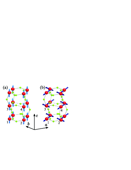
Figure 1: (Color online) Distribution of spin (a) and orbital (b) magnetic moments as obtained in the mean-field Hartree-Fock calculations for the low-energy model of YTiO₃.t2g The titanium atoms are indicated by the big red (dark) spheres and the oxygen atoms are indicated by the small green (grey) spheres. For the sake of clarity, the arrows for the orbital magnetic moments were scaled in order to have the same length as for the spin magnetic moments.

In this case, the vector of the spin magnetic moment at the site $1$ is $(-$$0.021,-$$0.127,\,0.986)$ $\mu_{\rm B}$ and the vector $\boldsymbol{\mu}^{0}$ of orbital magnetic moment is $(-$$0.033,-$$0.001,-$$0.018)$ $\mu_{\rm B}$. Therefore, the net local orbital magnetic moment ${\cal M}^{0}_{c}$ (per one primitive cell of YTiO₃, containing four Ti atoms) is $-$$0.072$ $\mu_{\rm B}$ (Table 1). As was explained above, it is parallel to the $\boldsymbol{c}$ axis.

Table 1: Different contributions to the net orbital magnetic moment, as obtained in the mean-field Hartree-Fock calculations for the low-energy model: the local moment $\boldsymbol{\cal M}^{0}$, given by periodic part of the orbital momentum operator in the Wannier basis, and two itinerant contributions, due to the local and itinerant circulation ($\Delta\boldsymbol{\cal M}^{LC}$ and $\boldsymbol{\cal M}^{IC}$, respectively). All values are in $\mu_{\textrm{B}}$ per one primitive cell, containing four transition-metal sites.

Compound	Direction	$\boldsymbol{\cal M}^{0}$	$\Delta\boldsymbol{\cal M}^{LC}$	$\boldsymbol{\cal M}^{IC}$	$\Delta\boldsymbol{\cal M}^{LC}+\boldsymbol{\cal M}^{IC}$
YTiO3 ($Pbnm$)	$||\boldsymbol{c}$	$-0.072$	$-1.22\cdot 10^{-5}$	$\phantom{-}2.63\cdot 10^{-4}$	$\phantom{-}2.50\cdot 10^{-4}$
LaMnO3 ($Pbnm$)	$||\boldsymbol{c}$	$-0.032$	$\phantom{-}1.05\cdot 10^{-4}$	$-2.28\cdot 10^{-4}$	$-1.23\cdot 10^{-4}$
YVO3 ($Pbnm$)	$||\boldsymbol{a}$	$-0.004$	$-6.75\cdot 10^{-4}$	$-1.30\cdot 10^{-4}$	$-8.05\cdot 10^{-4}$
YVO3 ($P2_{1}/a$)	$||\boldsymbol{b}$	$-0.020$	$\phantom{-}3.30\cdot 10^{-6}$	$-2.29\cdot 10^{-5}$	$-1.96\cdot 10^{-5}$

Then, we evaluate the itinerant correction $\Delta\boldsymbol{\cal M}$, resulting from the local and itinerant circulation terms. These results are summarized in Table 1. As expected, the projections of $\Delta\boldsymbol{\cal M}$ onto the orthorhombic $\boldsymbol{a}$ and $\boldsymbol{b}$ axes are identically equal to zero. The $\boldsymbol{c}$ projection ($\Delta{\cal M}_{c}$) is finite. However, it is more than two orders of magnitude smaller than ${\cal M}^{0}_{c}$ and, therefore, can be safely neglected. In principle, this result is also anticipated for the considered transition-metal oxides, which are frequently regarded as Mott insulators and in which the magnetically active $3d$ states are relatively well localized.

Nevertheless, it is interesting to gain some insight by investigating the origin of such a small value. For these purposes we analyze the integrand

$$\Delta\boldsymbol{\cal M}(\textbf{k})=\frac{e}{2\hbar c}\,\mathrm{Im}\sum_{n}\langle\partial_{\textbf{k}}c_{n\textbf{k}}|\times(\hat{H}_{\textbf{k}}+E_{n\textbf{k}})|\partial_{\textbf{k}}c_{n\textbf{k}}\rangle$$

of

$$\Delta\boldsymbol{\cal M}=\int_{BZ}\frac{d\textbf{k}}{\Omega}\,\Delta\boldsymbol{\cal M}(\textbf{k})$$

and plot it along high-symmetry directions of the BZ (see Fig. 2).

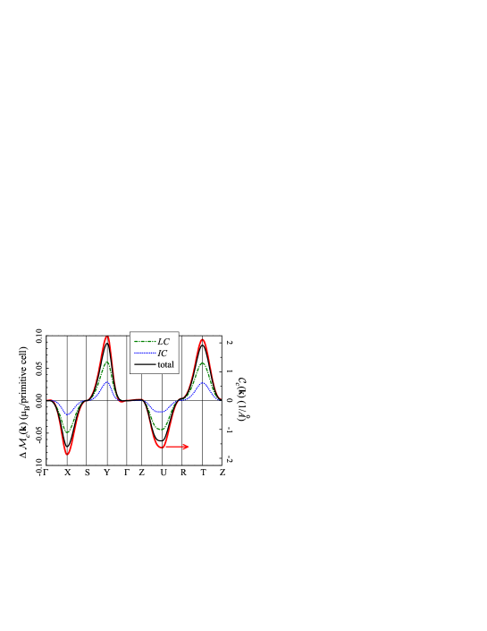
Figure 2: (Color online) Behavior of itinerant contributions to the net orbital magnetic moment in YTiO₃ (left axis) and corresponding Chern invariant (right axis) in the reciprocal space, along high-symmetry directions of the Brillouin zone. Two partial contributions to the net orbital moment, associated with the local ($\Delta\boldsymbol{\cal M}^{LC}$) and itinerant ($\boldsymbol{\cal M}^{IC}$) circulation are denoted as $LC$ and $IC$, respectively, and the sum of these two contributions is denoted as ‘total’.

Notations of the high-symmetry points of the BZ were taken from the book of Bradley and Cracknell.BradlayCracknell We obtained that two components, $\Delta{\cal M}_{a}(\textbf{k})$ and $\Delta{\cal M}_{b}(\textbf{k})$, are identically equal to zero in each k-point, while $\Delta{\cal M}_{c}(\textbf{k})$ can be finite and, moreover, strongly depend on k. This behavior is consistent with the G_a-A_b-F_c symmetry of the magnetic ground state.remark1 $\Delta{\cal M}_{c}(\textbf{k})$ reaches its maximal value of $0.088$ $\mu_{\textrm{B}}$ in the point $\textrm{Y}=(0,\frac{1}{2},0)$ of the BZ (in units of reciprocal lattice translations), which is comparable with ${\cal M}^{0}_{c}$. Thus, the individual contributions $\Delta{\cal M}_{c}(\textbf{k})$ can be large. However, there is also a large cancelation between positive and negative contributions to $\Delta{\cal M}_{c}$ around the Y and $\textrm{X}=(\frac{1}{2},0,0)$ points, respectively. Similar situation occurs at the BZ boundary $k_{c}=\frac{1}{2}$, where again the large positive contribution around $\textrm{T}=(0,\frac{1}{2},\frac{1}{2})$ is nearly canceled by the negative contribution around $\textrm{U}=(\frac{1}{2},0,\frac{1}{2})$. This result is summarized in Fig. 3,

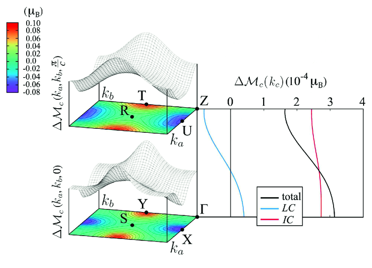
Figure 3: Left panel: Three-dimensional plot of $\Delta{\cal M}_{c}(\textbf{k})\equiv\Delta{\cal M}_{c}(k_{a},k_{b},k_{c})$ for $k_{c}=0$ and $\frac{1}{2}$ in the case of YTiO₃. Right panel: the $k_{c}$-dependence of $\Delta{\cal M}_{c}(k_{c})$, obtained after the integration of $\Delta{\cal M}_{c}(\textbf{k})$ over $k_{a}$ and $k_{b}$, and its partial contributions associated with local and itinerant circulation terms ($LC$ and $IC$, respectively).

where we plot $\Delta{\cal M}_{c}(k_{a},k_{b},k_{c})$ for $k_{c}=0$ and $\frac{1}{2}$, as well as the integrated value

$$\Delta{\cal M}_{c}(k_{c})=\frac{|\boldsymbol{a}||\boldsymbol{b}|}{4\pi^{2}}\int_{-\pi/a}^{\pi/a}dk_{a}\int_{-\pi/b}^{\pi/b}dk_{b}\,\Delta{\cal M}_{c}(k_{a},k_{b},k_{c}).$$

One can clearly see that $\Delta{\cal M}_{c}(k_{a},k_{b},k_{c})$ only weakly depends on $k_{c}$. For each $k_{c}$, there is a strong cancelation of the positive and negative contributions to $\Delta{\cal M}_{c}(k_{a},k_{b},k_{c})$, arising from $\textbf{k}=(0,\frac{1}{2},k_{c})$ and $(\frac{1}{2},0,k_{c})$, respectively. This cancelation readily explains the small value of $\Delta{\cal M}_{c}(k_{c})$. Finally, the integration of $\Delta{\cal M}_{c}(k_{c})$ over $k_{c}$ yields the total value of $\Delta{\cal M}_{c}$, reported in Table 1. Thus, the small value of $\Delta{\cal M}_{c}$ is the result of strong cancelation of relatively large contributions $\Delta{\cal M}_{c}(\textbf{k})$, coming from different parts of the BZ. This is the reason why we consider $\Delta\boldsymbol{\cal M}$ as an itinerant quantity. Moreover, the strong k-dependence of $\Delta\boldsymbol{\cal M}$ implies that after the Fourier transformation to the real space, in addition to the small site-diagonal component, this quantity will have a large nonlocal (or off-diagonal with respect to the atomic sites) part. Since the k-dependence is smooth, this Fourier series will converge and such a real-space analysis can be justified.

As was already pointed out in Sec. II, this behavior is closely related to that of the Chern invariants. For our purposes, it is convenient to rewrite $\boldsymbol{\cal C}$ in the following form:

$$\boldsymbol{\cal C}=\frac{1}{\Omega}\int_{BZ}d\textbf{k}\,\boldsymbol{\cal C}(\textbf{k}),$$

where

$$\boldsymbol{\cal C}(\textbf{k})=-\frac{\Omega}{2\pi}\mathrm{Im}\sum_{n}\langle\partial_{\textbf{k}}c_{n\textbf{k}}|\times|\partial_{\textbf{k}}c_{n\textbf{k}}\rangle.$$

For the normal insulators, $\boldsymbol{\cal C}$ is zero, and this property is perfectly reproduced by our calculations. However, due to the specific symmetry of the G_a-A_b-F_c ground state of YTiO₃,remark1 the integrand ${\cal C}_{c}(\textbf{k})$ can be finite in the individual k-points, while two other projections of $\boldsymbol{\cal C}(\textbf{k})$ onto the orthorhombic $\boldsymbol{a}$ and $\boldsymbol{b}$ axes are identically equal to zero. Furthermore, the k-dependence of ${\cal C}_{c}(\textbf{k})$ is very close to that of $\Delta{\cal M}_{c}(\textbf{k})$ (see Fig. 2). Thus, in the case of Chern invariant ${\cal C}_{c}(\textbf{k})$, the contributions from different parts of the BZ exactly cancel each other. However, in the expression for $\Delta{\cal M}_{c}$, the k-dependence of ${\cal C}_{c}(\textbf{k})$ for each band is additionally modulated with k-dependent quantities $\hat{H}_{\textbf{k}}$ and $E_{n\textbf{k}}$, that leads to a small but finite value of $\Delta{\cal M}_{c}$ (see Table 1). It also explains why $\Delta{\cal M}^{LC}_{c}(\textbf{k})$ and ${\cal M}^{IC}_{c}(\textbf{k})$ reveal very similar k-dependence: in both cases, it is dictated by the k-dependence of ${\cal C}_{c}(\textbf{k})$, which appears to be more fundamental quantity.

V.2 LaMnO₃

LaMnO₃ is another compound, crystallizing in the orthorhombic $Pbnm$ structure.LaMnO3exp It has the same G_a-A_b-F_c type of the magnetic ground state, which is realized below $T_{\rm N}\approx$ 140 K.Matsumoto This magnetic ground state was successfully reproduced in our mean-field HF calculations for the low-energy model. The basic difference from YTiO₃ is that the spin magnetic structure is nearly A-type antiferromagnetic (AFM) and the FM canting of spins in the $\boldsymbol{c}$ direction is really small. In this sense, LaMnO₃ is the canonical weak ferromagnet. Nevertheless, the orbital magnetic structure is strongly deformed: in comparison with the spin one, there is a large deviation from the collinear A-type AFM alignment and an appreciable canting of the orbital magnetic moments in the direction of $\boldsymbol{a}$ and $\boldsymbol{c}$, which can be seen even visually in Fig. 4.

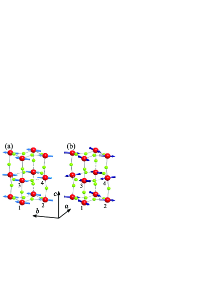
Figure 4: (Color online) Distribution of spin (a) and orbital (b) magnetic moments as obtained in the mean-field Hartree-Fock calculations for the low-energy model of LaMnO₃. The manganese atoms are indicated by the big red (dark) spheres and the oxygen atoms are indicated by the small green (grey) spheres. For the sake of clarity, the arrows for the orbital magnetic moments were scaled in order to have the same length as for the spin magnetic moments.

The vector of spin magnetic moment at the site 1 is $(\,0.354,\,3.952,\,0.111)$ $\mu_{\rm B}$ and the one of orbital magnetic moment $\boldsymbol{\mu}^{0}$ is $(-$$0.030,-$$0.057,-$$0.008)$ $\mu_{\rm B}$. Thus, the net orbital magnetic moment $\boldsymbol{\cal M}^{0}$ is $-$$0.032$ $\mu_{\rm B}$ (Table 1).

The behavior of $\Delta\boldsymbol{\cal M}(\textbf{k})$ is qualitatively the same as in YTiO₃: it has similar structure and similar type of cancelation between different parts of the BZ (Fig. 5).

Figure 5: (Color online) Behavior of itinerant contributions to the net orbital magnetic moment in LaMnO₃ (left axis) and corresponding Chern invariant (right axis) in the reciprocal space, along high-symmetry directions of the Brillouin zone. Two partial contributions to the net orbital moment, associated with the local ($\Delta\boldsymbol{\cal M}^{LC}$) and itinerant ($\boldsymbol{\cal M}^{IC}$) circulation are denoted as $LC$ and $IC$, respectively, and the sum of these two contributions is denoted as ‘total’.

Taking into account that YTiO₃ and LaMnO₃ have the same type of crystal structure and the magnetic ground state, such similarity is not surprising. The main difference is the magnitude of the effect, which is much more pronounced in LaMnO₃: the values of $\Delta{\cal M}_{c}(\textbf{k})$ in the Y and T points are $0.154$ $\mu_{\rm B}$ and $0.159$ $\mu_{\rm B}$, respectively, which exceed ${\cal M}^{0}_{c}$ by factor five. However, there is again a strong cancelation with the negative contributions around the X and U points of the BZ, which, after the integration, leads to the small value of $\Delta{\cal M}_{c}$. Moreover, in LaMnO₃ there is a partial cancelation between $LC$ and $IC$ contributions to $\Delta{\cal M}_{c}$ (see Table 1).

Like in YTiO₃, the k-dependence of $\Delta{\cal M}_{c}(\textbf{k})$ in LaMnO₃ follows the form of ${\cal C}_{c}(\textbf{k})$ (Fig. 5). Nevertheless, one interesting aspect is that the amplitude of ${\cal C}_{c}(\textbf{k})$ in LaMnO₃ is smaller than in YTiO₃ (Fig. 2), while for $\Delta{\cal M}_{c}(\textbf{k})$ the situation is exactly the opposite. This difference may be related to the number of occupied bands (16 in the case of LaMnO₃ versus 4 in the case of YTiO₃). Thus, the amplitude of $\Delta{\cal M}_{c}(\textbf{k})$ may be larger in LaMnO₃ because the number of occupied bands is larger. Another possibility is that the contributions of different bands cancel each other and this cancelation occurs in a different way in the case of ${\cal C}_{c}(\textbf{k})$ and $\Delta{\cal M}_{c}(\textbf{k})$.

V.3 YVO₃

YVO₃ has two crystallographic modifications: orthorhombic $Pbnm$, which is realized below 77 K, and monoclinic $P2_{1}/a$ above 77 K (in our calculations, we use the experimental structure parameters at 65 K and 100 K, respectively).YVO3exp The magnetic structure, realized in the orthorhombic $Pbnm$ phase is F_a-C_b-G_c (Fig. 6). According to the mean-field HF calculations for the low-energy model, the vector of spin magnetic moment at the site 1 is $(-$$0.016,\,0,\,1.969)$ $\mu_{\rm B}$ and the vector of orbital magnetic moment is $(-$$0.001,\,0.001,-$$0.186)$ $\mu_{\rm B}$. Thus, the $\boldsymbol{c}$ projection clearly dominates, while two other projections are substantially smaller. The net orbital magnetic moment is only $-$$0.004$ $\mu_{\rm B}$, which is parallel to the orthorhombic $\boldsymbol{a}$ axis.

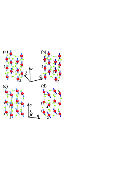
Figure 6: (Color online) Distribution of spin (a and c) and orbital (b and d) magnetic moments as obtained in the mean-field Hartree-Fock calculations for the low-energy model of YVO₃ in the orthorhombic (a and b) and monoclinic (c and d) phases. The vanadium atoms are indicated by the big red (dark) spheres and the oxygen atoms are indicated by the small green (grey) spheres. For the sake of clarity, the arrows for the orbital magnetic moments in the sublattice (1,2) were scaled in order to have the same length as for the spin magnetic moments. The orbital magnetic moments in the sublattice (3,4) are additionally quenched by stronger crystal field.

The monoclinic phase of YVO₃ has two inequivalent pairs of V sites, which are denoted in Fig. 6 as (1,2) and (3,4). Within each pair, the $\boldsymbol{a}$ and $\boldsymbol{c}$ projections of the magnetic moments are coupled antiferromagnetically, while the $\boldsymbol{b}$ projection is ferromagnetic. According to the mean-field HF calculations for the low-energy model, the vectors of spin magnetic moments at the sites 1 and 3 are $(-$$0.850,\,0.077,\,1.785)$ $\mu_{\rm B}$ and $(-$$0.875,-$$0.032,\,1.764)$ $\mu_{\rm B}$, respectively, and the vectors of orbital magnetic moments are $(\,0.074,-$$0.046,-$$0.173)$ $\mu_{\rm B}$ and $(\,0.043,\,0.036,-$$0.073)$ $\mu_{\rm B}$, respectively. The local orbital magnetic moments in the sublattice (3,4) are substantially smaller due to additional quenching by stronger crystal field (see Ref. t2g, for details). Thus, there is a partial cancelation of the FM magnetization between two sublattices. However, due to the additional quenching in the sublattice (3,4), this cancelation is not complete and the system remains weakly ferromagnetic. The net orbital magnetic moment $\boldsymbol{\cal M}^{0}$ is $-$$0.02$ $\mu_{\rm B}$, which is parallel to the monoclinic $\boldsymbol{b}$ axis. The directions of the net magnetic moment and, therefore, the type of the magnetic ground state in the orthorhombic and monoclinic phases are well consistent with the experimental data.Ren

The type of the magnetic ground state in orthorhombic YVO₃ is different from the one of YTiO₃ and LaMnO₃. As a result, the k-dependence of $\boldsymbol{\cal C}(\textbf{k})$ and $\Delta\boldsymbol{\cal M}(\textbf{k})$ is also different. Since the net magnetic moment is parallel to the orthorhombic $\boldsymbol{a}$ axis, only $\boldsymbol{a}$ projection of $\Delta\boldsymbol{\cal M}$ is finite, while two other projections are identically equal to zero. Then, $\Delta{\cal M}_{a}(\textbf{k})$ reaches the maximal value of $0.099$ $\mu_{\rm B}$ in the X point of the BZ (Fig. 7),

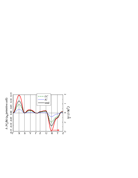
Figure 7: (Color online) Behavior of itinerant contributions to the net orbital magnetic moment in orthorhombic YVO₃ (left axis) and corresponding Chern invariant (right axis) in the reciprocal space, along high-symmetry directions of the Brillouin zone. Two partial contributions to the net orbital moment, associated with the local ($\Delta\boldsymbol{\cal M}^{LC}$) and itinerant ($\boldsymbol{\cal M}^{IC}$) circulation are denoted as $LC$ and $IC$, respectively, and the sum of these two contributions is denoted as ‘total’.

which exceeds the net local magnetic moment ${\cal M}^{0}_{a}$ by more than one order of magnitude (Table 1). There are other positive contributions, originating from the X, $\textrm{Z}=(0,0,\frac{1}{2})$, and U points of the BZ. Nevertheless, they are well compensated by the negative contributions, coming from the T and $\textrm{R}=(\frac{1}{2},\frac{1}{2},\frac{1}{2})$ points of the BZ, that again results in the small value of $\Delta{\cal M}_{a}$ (Table 1). This behavior is totally consistent with the form of ${\cal C}_{a}(\textbf{k})$.

A completely different type of cancelation occurs in the monoclinic phase of YVO₃. In this case, the net orbital moment is parallel to the monoclinic $\boldsymbol{b}$ axis (Table 1), and $\Delta{\cal M}_{b}(\textbf{k})$ has the largest magnitude in the plane $k_{c}=\frac{1}{2}$, where the region of positive values around the point $\textrm{E}=(\overline{\frac{1}{2}},\frac{1}{2},\frac{1}{2})$ is nearly canceled by the region of negative values around the point $\textrm{D}=(\overline{\frac{1}{2}},0,\frac{1}{2})$ (Fig. 8).

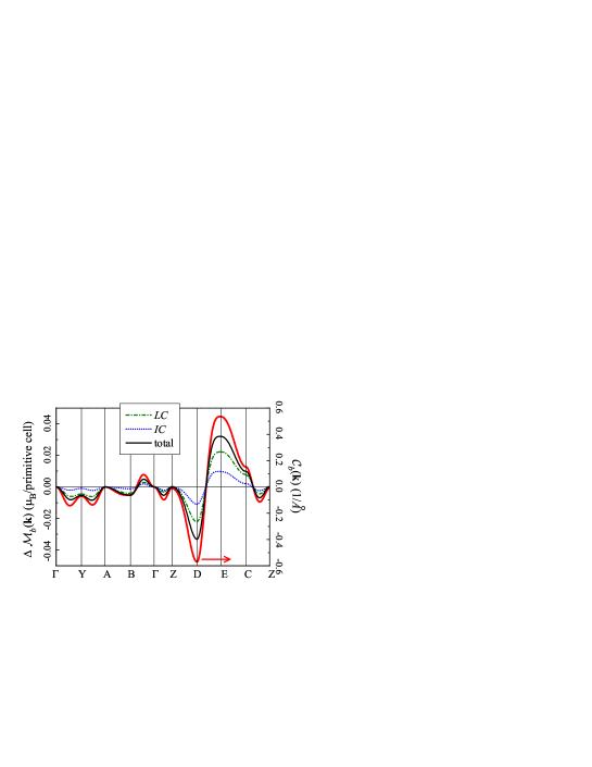
Figure 8: (Color online) Behavior of itinerant contributions to the net orbital magnetic moment in monoclinic YVO₃ (left axis) and corresponding Chern invariant (right axis) in the reciprocal space, along high-symmetry directions of the Brillouin zone. Two partial contributions to the net orbital moment, associated with the local ($\Delta\boldsymbol{\cal M}^{LC}$) and itinerant ($\boldsymbol{\cal M}^{IC}$) circulation are denoted as $LC$ and $IC$, respectively, and the sum of these two contributions is denoted as ‘total’.

This behavior is again consistent with the form of ${\cal C}_{b}(\textbf{k})$ and explains the small value of integrated $\Delta{\cal M}_{b}$ in Table 1.

VI Conclusions

We have applied the modern theory of orbital magnetization to the series of characteristic distorted perovskite transition-metal oxides with a net FM moment in the ground state. Our applications cover the examples of canted (but yet robust) ferromagnetism in orthorhombic YTiO₃ as well as weak ferromagnetism caused by either antisymmetric Dzyalishinskii-Moriya interactions in orthorhombic LaMnO₃ and YVO₃ or imperfect cancelation of magnetic moments between two crystallographic sublattices in monoclinic YVO₃. Our numerical calculations suggest that, for all these compounds, the orbital magnetization can be well described by the “standard” expression (1), in terms of the angular momentum operator and the site-diagonal density matrix, while all the “itinerant” corrections, originating from the modern theory, are negligibly small. Nevertheless, the smallness of these corrections is the result of rather nontrivial cancelation of relatively large contributions coming from different parts of the BZ.

There is a big difference in the behavior of orbital magnetization and ferroelectric (FE) polarization in improper multiferroics. In the latter case, the inversion symmetry is broken by some complex magnetic order, while the crystal structure itself, to a good approximation, can be regarded as centrosymmetric. Then, if the magnetic sites are located in the centers of inversion, Eq. (8) yields $\langle\phi_{\alpha^{\prime}}(\textbf{r}-\textbf{R})|\textbf{r}-\textbf{R}|\phi_{\alpha}(\textbf{r}-\textbf{R})\rangle=0$, which means that there is no “local FE polarization”, associated with the basis functions of the magnetic sites. Finite value of the FE polarization in this case is related to the k-dependence of the coefficients $\{c_{n\textbf{k}}\}$ of expansion of the Bloch eigenfunctions over the basis functions and can be obtained by applying the Berry-phase theory only for $\{c_{n\textbf{k}}\}$.FE_model ; PRB13 In this sense, and using an analogy with the modern theory for the orbital magnetization, one can say that the FE polarization in improper multiferroics is entirely itinerant quantity and can even serve as the measure of itineracy of magnetic system.PRB13

The behavior of orbital magnetization in the normal FM insulators is fundamentally different. In this case, there are finite local magnetic moments, which are expressed in terms of matrix elements of the angular momentum operator in the Wannier basis, and these local magnetic moments provide the main contribution to the net orbital magnetic moment. The itinerant corrections $\Delta\boldsymbol{\cal M}$ to this net FM moment, originating from the k-dependence of $\{c_{n\textbf{k}}\}$, are considerably smaller. Thus, the orbital magnetic moment is mainly a local quantity.

The form of $\boldsymbol{\cal M}(\textbf{k})$ in the reciprocal space follows the behavior of Chern invariants. Although the full integral over the BZ is small (or identically equals to zero in the case of Chern invariants), the integrand itself is finite and, moreover, can be strongly k-dependent. By tracing this discussion back to the real space by means of the Fourier transform, this would mean that the considered quantities will have nonlocal (or off-diagonal with respect to the atomic sites) contributions and, for the normal insulators studied in this work, these nonlocal contributions will be substantially larger than the local (or site-diagonal) ones. This is one of the most interesting aspects of the modern theory of the orbital magnetization, which raises many new questions. Particularly, can these large nonlocal contributions be measured or can they contribute to other properties?

Another interesting issue is related to the first fundamental question – the direction for the improvement of SDFT. Will this large and essentially nonlocal part of the orbital magnetization contribute to the exchange-correlation energy, for instance – in the framework of frequently discussed in this context current SDFT?VignaleRasolt ; Ebert ; ShiPRL Unfortunately, the explicit form of the exchange-correlation energy in terms of these orbitals currents is largely unknown, and today it is an open (but very interesting) question whether such theory can also improve the description of local orbital magnetization, which is probed by many experiments. As was pointed our in the Introduction, so far the dominant point of view was that the orbital magnetization is a local quantity and the main processes, which are missing in practical DFT calculations and which are responsible for the agreement with the experimental data can be also formulated in the local (or site-diagonal) form.OPB ; Norman ; LDAU ; Minar In the light of this new funding, how general is this conclusion and how important are the non-local processes, associated with the appreciable k-dependence of the itinerant part of the orbital magnetization?

Acknowledgements. This work is partly supported by the grant of the Ministry of Education and Science of Russia N 14.A18.21.0889.

References

- (1) R. M. White, Quantum Theory of Magnetism (Springer-Verlag, Berlin, 2007).
- (2) Magnetism and Synchrotron Radiation, Springer Proceedings in Physics Vol. 133, edited by E. Beaurepaire, H. Bulou, F. Scheurer, and J.-P. Kappler (Springer-Verlag, Berlin, 2010) and references therein.
- (3) G. H. Lander, Physica Scripta 44, 33 (1991).
- (4) The relativistic SO coupling is proportional to gradient of the scalar potential.White Therefore, in order to produce finite SO coupling, this potential should be position-dependent (or “inhomogeneous”). The external vector potential is also position-dependent, even for the uniform magnetic field.
- (5) G. Vignale and M. Rasolt, Phys. Rev. Lett. 59, 2360 (1987); G. Vignale and M. Rasolt, Phys. Rev. B 37, 10685 (1988).
- (6) H. J. F. Jansen, Phys. Rev. B 43, 12025 (1991).
- (7) O. Eriksson, M. S. S. Brooks, and B. Johansson, Phys. Rev. B 41, 7311 (1990); O. Eriksson, B. Johansson, R. C. Albers, A. M. Boring, and M. S. S. Brooks, ibid. 42, 2707 (1990).
- (8) M. R. Norman, Phys. Rev. Lett. 64, 1162 (1990); M. R. Norman, Phys. Rev. B 44, 1364 (1991).
- (9) I. V. Solovyev, A. I. Liechtenstein, and K. Terakura, Phys. Rev. Lett. 80, 5758 (1998); I. V. Solovyev, ibid. 95, 267205 (2005).
- (10) J. Minár, J. Phys.: Condens. Matter 23, 253201 (2011) and references therein.
- (11) H. Ebert, M. Battocletti, and E. K. U. Gross, Europhys. Lett. 40, 545 (1997).
- (12) R. D. King-Smith and D. Vanderbilt, Phys. Rev. B 47, 1651 (1993); D. Vanderbilt and R. D. King-Smith, ibid. 48, 4442 (1993).
- (13) R. Resta, J. Phys.: Condens. Matter 22, 123201 (2010).
- (14) D. Xiao, J. Shi, and Q. Niu, Phys. Rev. Lett. 95, 137204 (2005).
- (15) T. Thonhauser, D. Ceresoli, D. Vanderbilt, and R. Resta, Phys. Rev. Lett. 95, 137205 (2005).
- (16) D. Ceresoli, T. Thonhauser, D. Vanderbilt, and R. Resta, Phys. Rev. B 74, 024408 (2006).
- (17) J. Shi, G.Vignale, D. Xiao, and Q. Niu, Phys. Rev. Lett. 99, 197202 (2007).
- (18) T. Thonhauser, Int. J. Mod. Phys. B 25, 1429 (2011).
- (19) F. D. M. Haldane, Phys. Rev. Lett. 61, 2015 (1988).
- (20) D. Ceresoli and R. Resta, Phys. Rev. B 76, 012405 (2007).
- (21) D. Ceresoli, U. Gerstmann, A. P. Seitsonen, and F. Mauri, Phys. Rev. B 81, 060409 (2010); M. G. Lopez, D. Vanderbilt, T. Thonhauser, and I. Souza, ibid. 85, 014435 (2012).
- (22) S. Coh, D. Vanderbilt, A. Malashevich, and I. Souza, Phys. Rev. B 83, 085108 (2011).
- (23) I. Dzyaloshinsky, J. Chem. Phys. Solids 4, 241 (1958); T. Moriya, Phys. Rev. 120, 91 (1960).
- (24) D. Treves, Phys. Rev. 125, 1843 (1962).
- (25) I. V. Solovyev, J. Phys.: Condens.Matter 20, 293201 (2008).
- (26) D. J. Thouless, Topological Quantum Numbers in Nonrelativistic Physics (World Scientific, Singapore, 1998).
- (27) I. V. Solovyev, Phys. Rev. B 74, 054412 (2006); I. V. Solovyev, J. Comput. Electron. 10, 21 (2011).
- (28) I. Solovyev, J. Phys. Soc. Jpn. 78, 054710 (2009).
- (29) O. K. Andersen, Phys. Rev. B 12, 3060 (1975); O. Gunnarsson, O. Jepsen, and O. K. Andersen, ibid. 27, 7144 (1983); O. K. Andersen, Z. Pawlowska, and O. Jepsen, ibid. 34, 5253 (1986).
- (30) Supplemental materials [details of derivation of Eqs. (9)-(10)].
- (31) A. C. Komarek, H. Roth, M. Cwik, W.-D. Stein, J. Baier, M. Kriener, F. Bourée, T. Lorenz, and M. Braden, Phys. Rev. B 75, 224402 (2007).
- (32) C. J. Bradley and A. P. Cracknell, The Mathematical Theory of Symmetry in Solids (Clarendon Press, Oxford, 1972).
- (33) In the Ga-Ab-Fc ground state, the twofold rotation around the orthorhombic axis enters as it is, while two other rotations around the orthorhombic and axes enter in the combination with the time inversion.
- (34) J. B. A. A. Elemans, B. van Laar, K. R. van der Veen, and B. O. Loopstra: J. Sol. State Chem. 3, 238 (1971).
- (35) G. Matsumoto, J. Phys. Soc. Jpn. 29, 606 (1970).
- (36) G. R. Blake, T. T. M. Palstra, Y. Ren, A. A. Nugroho, and A. A. Menovsky, Phys. Rev. B 65, 174112 (2002).
- (37) Y. Ren, T. T. M. Palstra, D. I. Khomskii, E. Pellegrin, A. A. Nugroho, A. A. Menovsky, and G. A. Sawatzky, Nature 396, 441 (1998). Note that the experimental net magnetization in the orthorhombic phase is parallel to the axis, that is totally consistent with our calculations. The experimental magnetization in the monoclinic phase is also parallel to the direction in the orthorhombic setting, which corresponds to the direction in the monoclinic setting, in agreement with our calculations.
- (38) I. V. Solovyev, Phys. Rev. B 83, 054404 (2011); I. V. Solovyev, M. V. Valentyuk, and V. V. Mazurenko, ibid. 86, 144406 (2012).
- (39) I. V. Solovyev and S .A. Nikolaev, Phys. Rev. B 87, 144424 (2013).