Two dimensional Leidenfrost Droplets in a Hele Shaw Cell

Abstract

We experimentally and theoretically investigate the behavior of Leidenfrost droplets inserted in a Hele-Shaw cell. As a result of the confinement from the two surfaces, the droplet has the shape of a flattened disc and is thermally isolated from the surface by the two evaporating vapor layers. An analysis of the evaporation rate using simple scaling arguments is in agreement with the experimental results. Using the lubrication approximation we numerically determine the shape of the droplets as a function of its radius. We furthermore find that the droplet width tends to zero at its center when the radius reaches a critical value. This prediction is corroborated experimentally by the direct observation of the sudden transition from a flattened disc into an expending torus. Below this critical size, the droplets are also displaying capillary azimuthal oscillating modes reminiscent of a hydrodynamic instability.

I Introduction

In spite of its discovery in the late 19 th century leiden , the Leidenfrost phenomenon is still today the subject of numerous studies for two essential reasons. The first reason is related to the strong decrease of the thermal exchange between the solid and the liquid due to the presence of low thermal conductivity vapor layers: this situation is of importance for example in metallurgy to control the cooling of metals bernardin or in nuclear reactor safety vandam . The second is fundamental and related to the fact that a Leidenfrost droplet may be considered as an ideal realization of a perfect non-wetting system clanet ; quere . These droplets have shown rich and unexpected behaviors quere . For example drops on periodic patterned surface display a drift due to the spatial symmetry breaking. Furthermore possible applications of Leidenfrost droplets might be the transport of liquid in the milli-fluidic or micro-fluidic area tabeling . For example low pressure Leidenfrost droplets have been shown recently to be stable at room temperature and could be subsequently potential receptor of particles in solution pression . Surprisingly, to our knowledge no studies have been devoted yet to the Leidenfrost effect in a 2d confined geometry. This is somehow unexpected because such a complex phenomenon should display new properties as the spatial dimension is reduced. The aim of this paper is thus to investigated a simple situation representative of the effect of spatial confinement on the Leidenfrost droplets. These droplets are inserted in a horizontal Hele-Shaw cell whose gap is smaller than the capillary length $\kappa^{-1}=\sqrt{\gamma/\rho_{l}g}$ with $\gamma$ being the surface tension, $\rho_{l}$ the liquid density and $g$ the acceleration of gravity. As a result of the confinement from the two surfaces the drop takes the shape of a flattened saucer-like disc which floats between two vapor layers. These drops are quasi thermally isolated from the surface by the evaporating vapor layers and they display undulating star-like shapes. In this Article, we first describe our experimental set-up and we describe the dynamic of evaporation by a simple model which takes into account the Poiseuille flow in the vapor layer. This model is in agreement with the experimental results for the global evaporation rates. We then discuss the vertical profile of the drop using a theoretical model which results from the balance between surface tension and the Poiseuille flow in the vapor layer. We observed that the droplets have a maximum radius $R_{c}$ beyond which they transform into a torus by the process of a hole nucleation and expansion at their center. These experimental results are confronted with our theoretical model and fall within a good agreement. We also report observations of large amplitude star-like undulation consisting of azimuthal oscillating capillary wave. The frequency of oscillations is measured and is found to be close to the frequency of Rayleigh capillary wave of droplets. Finally, we discuss possible mechanisms at the origin of the instability leading to star-like oscillations of the droplets.

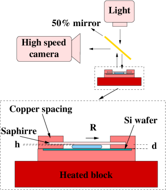
Figure 1: Experimental set-up : a Hele-Shaw cell is heated at a controlled temperature $T_{P}$. A Leidenfrost droplet of radius $R$ is inserted between the two hot plates separated by a spacing $d$.

II Evaporation dynamic

II.1 Experimental results

Our experimental set-up is depicted in Fig.1. A heated copper block permits to control the temperature $T_{p}$ of two plates separated by a spacing of width $d$. This temperature is measured with a PT100 temperature sensor. The upper plate is made of sapphire whose optical and thermal properties permit us to visualize the droplet from the top through a semi-transparency mirror. The lower plate is covered with a silicon wafer. Images are recorded with a high speed camera with a frame rate varying between $60$ and $4000$ frames per second. As for classical Leidenfrost droplets we suppose that the liquid is at its boiling temperature $T_{b}$ and we denote $\Delta T=T_{p}-T_{b}$ the temperature difference between the hot plates and the droplet. For all the experiments, the plate temperature has been fixed to $T_{p}=300$ Celsius, giving a value of $\Delta T=200$ Celsius. A capillary is used to insert the ultra distilled water droplet into the Hele-Shaw cell. Different spacings $d$ have been used ranging between $d=0.3$ and $2$ mm.

We first investigate the dynamics of the evaporating droplets. The lifetime of the droplet is about ten seconds, one order of magnitude lower than usual Leidenfrost droplets and two orders of magnitude lower than low pressure Leidenfrost droplets pression . As illustrated on Fig. 2, the droplet is slowly evaporating and its radius $R$ is decreasing with time. An image analysis permits to record the evolution of $R$ with the time $t$, its value is deducted from the apparent area of the droplet viewed from the top. It is worth noticing that the shape of the drop is not necessary circular but presents some contour oscillations that will be discussed in the last section of this Article. We represent in Fig. 3 the time evolution of the radius $R$ for droplets inserted in three cells with different spacings : $d=0.3$, $0.5$ and $1{\rm\,mm}$. We clearly see that the lower the spacing the faster the evaporation of the droplet. The full lines correspond to a best-fit of the phenomenological model which is presented just below.

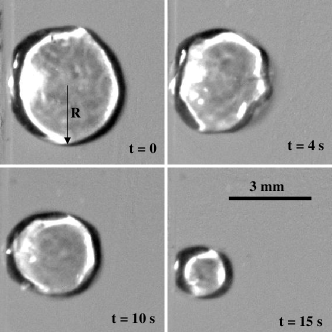
Figure 2: Snapshots of an evaporating droplet (top view) at different time. The spacing of the Hele-Shaw cell is of $1$ mm and the temperature of the plates is $T_{p}=300$ Celsius.

II.2 Phenomenological model

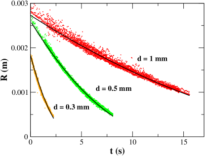
Figure 3: Droplet radius as a function of time for three different spacings $d=1$, $0.5$ and $d=0.3$ mm respectively in red, green and brown circles. The full lines correspond to the best fit to Eq. (9)

One of the difficulties in the Leidenfrost system consists in the determination of the thickness $h$ of the vapor film which is situated between the drop and the heated plates. In order to estimate $h$ we develop a model based on a simple scaling argument which applies to a flat droplet of radius $R$ as shown on Fig. 1. The vapor film thickness results from the balance between the pressure (driven by the Poiseuille flow produced by the local vapor evaporation) and the capillary surface tension effects. Energy conservation during the evaporation process (namely Stefan’s boundary condition on the liquid-vapor interface) and Fourier law for the heat transfer in the film yield the order of magnitude for the vertical velocity $w$ of the vapor near the surface of the droplet. It reads:

$$\rho_{v}Lw\propto\lambda\Delta T/h\,.$$ (1)

Here $L$ is the latent heat per unit mass, $\lambda$ is the thermal diffusivity coefficient, $\Delta T$ is the temperature difference between the hot plates and the droplet and $\rho_{v}$ is the density of the vapor. Mass conservation yields the following estimate for the magnitude of the horizontal velocity $u$ in terms of the vertical velocity $w$:

$$u/R\propto w/h\,.$$ (2)

Assuming a Poiseuille flow in the vapor in the lubrication regime leads to an horizontal pressure drop $\Delta P$ which scales as

$$\Delta P/R\propto\eta u/h^{2}\,,$$ (3)

where $\eta$ is the vapor film viscosity.

Finally, we note that the Laplace pressure $\Delta P$ between the drop and the gas reads:

$$\Delta P\propto\gamma/d\,,$$ (4)

Here we have neglected the small curvature term which is smaller by a factor $d/R$.

We obtain using Eqs. (1-4) a relation for the film height $h$ which reads:

$$h\propto R^{1/2}d^{1/4}\left(\frac{\eta\lambda\Delta T}{\rho_{v}L\gamma}\right)^{1/4}\,,$$ (5)

which can be rewritten simply as :

$$h\propto R^{1/2}d^{1/4}l^{1/4}\,,$$ (6)

where we have introduced a characteristic length $l$ defined as :

$$l=\frac{\eta\lambda\Delta T}{\rho_{v}L\gamma}\,.$$ (7)

As shown by Eq. (6), the width of the vapor layer $h$ can thus be deduced from the measured value $R$.

Furthermore we can also verify experimentally that the previous scaling holds by measuring the time evolution of the radius of the drop $R(t)$. The rate of evaporation of the droplet can be deduced from the outgoing flux of vapor and reads:

$$\rho_{l}\frac{d}{dt}(\pi R^{2}d)\propto 2\rho_{v}\pi R^{2}w\,.$$ (8)

Solving this differential equations using Eqs. (1) and (6) we obtain the evolution radius $R(t)$ as:

$$R(t)\propto(R_{0}^{1/2}-Ct)^{2}\,.$$ (9)

Here

$$C=\frac{\lambda\Delta T}{\rho_{l}Ll^{1/4}}d^{-5/4}\,.$$ (10)

As shown on Fig. 3, we compare the experimental measurements of the time evolution of the radius $R(t)$ with the theoretical prediction given in Eq. (9) for three different values of the spacing $d$. A satisfactory agreement is found between the theory and the experiments. We can infer the value of the constant $C$ from a best-fit adjustment of the data given on Fig. 3 using the time evolution for $R(t)$ given in Eq. (9). As shown on Fig. 4 the values of $C$ obtained lead to the expected dependence $C\propto d^{-5/4}$ as predicted by Eq. (10). It is worth noticing that the value of the pre-factor $\frac{\lambda\Delta T}{\rho_{l}Ll^{1/4}}$ found experimentally using the data shown on Fig. 3 is $2.9\times 10^{-7}{\rm m}^{1/2}\,{\rm s}^{-1}$. It is of same order than the one predicted $5.4\times 10^{-7}{\rm m}^{1/2}\,{\rm s}^{-1}$.
Here we have used the following values for the physical parameters: $\lambda=0.032\,{\rm J}\,{\rm s}^{-1}{\rm K}^{-1}$, $L=2.25\,10^{6}{\rm J}\,{\rm kg}^{-1}$, $\rho_{v}=0.81{\rm kg}\,{\rm m}^{-3}$, $\eta=1.3\,10^{-5}{\rm kg}\,{\rm m}^{-1}\,{\rm s}^{-1}$, $\kappa=\lambda/(L\rho_{v})$, $\Delta T=200\,{\rm Celsius}$, $\sigma=0.072\,{\rm J}{\rm m}^{-2}$ and $d=0.001{\rm m}$

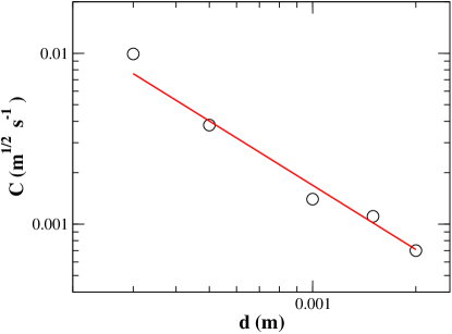
Figure 4: Values of the parameter $C$ as a function of the spacing $d$. The full line corresponds to the scaling law predicted in Eq. (10).

III Droplet shape and hole nucleation

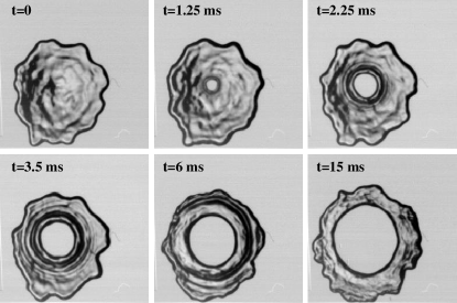
Figure 5: Images sequence of the hole nucleation and growth.

The previous analysis is based upon a strong hypothesis of a constant vapor thickness, both below and above the droplet. It has been recently shown that this hypothesis does not hold properly for 3D Leidenfrost droplet CRAS . Therefore we decided to perform a deeper theoretical analysis to predict the vapor layer profile in our confined geometry.

III.1 Lubrication model

Let the height of the vapor layer at the equator be $h_{0}$, the neck height $h_{n}$ and the radius of the droplet be $R$ as shown on Fig. 6. The two plates are held at temperature $T_{p}$ and are separated by a distance $d$, the temperature of the drop is $T_{b}$. Let $h(r)$ be the shape on the lower interface and $d-h(r)$ the shape of the upper interface.The balance between the surface tension effect and the Poiseuille flow leads to a variety of shapes which can described using the lubrication approximation. This approach has been used successfully in another context such as lens floating duchemin . The pressure $p$ in the vapor film just outside the drop is driven by the following equation as shown in Appendix A and reference CRAS :

$$\partial_{r}\left(\frac{rh^{3}}{12}\partial_{r}p\right)+\frac{r\eta\kappa\Delta T}{h(r)}=0\,,$$ (11)

where $\kappa=\lambda/(\rho_{v}L)$. Equation (11) derives from the incompressibility condition of the vapor and the Poisseuille hydrodynamic relation CRAS . The pressure in the vapor film just below the drop is given by:

$$p=p_{d}-\sigma\kappa\,.$$ (12)

Here $p_{d}$ is the pressure in the drop which is supposed to be constant, $\sigma$ is the surface tension and $\kappa$ is the mean curvature which reads:

$$\kappa=\partial_{s}\psi+\sin{\psi}/r\,.$$ (13)

Let us choose $d$ as the unit of length and $\sigma/d$ the pressure unit. in these units Eq. (11) reads:

$$\partial_{r}\left(\frac{rh^{3}}{12}\partial_{r}p\right)+\frac{r\alpha}{h}=0\,,$$ (14)

where $\alpha=\frac{\eta\kappa\delta T}{\sigma d}$ is a dimensionless parameter which depends on $d$.

Figure 6: sketch of a vertical cut of a drop. $h_{0}$, $h_{n}$ and $R$ are shown.

The lubrication Eq. (13, 14) can be reformulated in curvilinear coordinates as:

$$\partial_{s}h = \sin{\psi}\,,$$ (15)

$$\partial_{s}r = \cos{\psi}\,,$$ (16)

$$\partial_{s}\psi = \kappa-\sin{\psi}/r\,,$$ (17)

$$\partial_{s}\kappa = \kappa_{1}\,,$$ (18)

$$\partial_{s}\kappa_{1} = \frac{12\alpha\cos^{2}(\psi)}{h^{4}}-\frac{3\kappa_{1}h^{\prime}}{h}$$ (19)

$$-\frac{\kappa_{1}\left(r\psi^{\prime}\tan(\psi)+r^{\prime}\right)}{r}\,.$$

Here we have used the following geometric transformation $\partial_{r}=\partial_{s}\frac{\partial s}{\partial r}=\frac{\partial_{s}}{\cos(\psi)}$. The boundary conditions at $r=0$ read:

$$r(s=0) = 0\,,$$ (20)

$$h(s=0) = h_{0}\,,$$ (21)

$$\psi(0) = 0\,,$$ (22)

$$\kappa(0) = \kappa_{0}\,,$$ (23)

$$\partial_{s}\kappa(0) = 0\,.$$ (24)

The boundary conditions at $s=s_{max}$ which corresponds to the equator read:

$$r(s=s_{max}) = R\,,$$ (25)

$$h(s_{max}) = 1/2$$ (26)

$$\psi(s_{max}) = \pi/2$$ (27)

$$\partial_{s}\kappa(s_{max}) = 0$$ (28)

There are two free parameters $\kappa_{o}$ and $s_{max}$ which need to be adjusted in order to satisfy the boundary conditions defined in Eqs. (27) and (28). These equations can be solved using a standard shooting method. As shown in Fig. 7 we represent the shape of the drop for different values of the $h_{0}$,

Figure 7: Profile of a drop obtained by numerical resolutions of Eqs. (15-19) for 6 different values o the parameters $h_{0}$. Top $h_{0}=0.001{\rm mm}$, bottom $h_{0}=0.5{\rm mm}$. The horizontal axis is $r$, the vertical axis is the $z$ axis. The vertical distance $d$ between the two plates is $1$ mm. The bottom curve represent the the curve for which $R=R_{c}$.

we find that there exists a critical radius $R_{c}$ beyond which a simply connected drop cannot exist as shown for example on the bottom profile displayed on Fig. 7. Even though the direct measurement of vertical profile of the droplet are not possible, we have estimated the value of the vapor layer $h$ by proceeding in the following manner. Using the relation obtained in Eq. 5 we can estimate the value of $h$ by a measurement of $R$. Here the value for the pre-factor in Eq. 5 is deducted from the experimental measurement of the constant $C$, the pre-factor in Eq. 10 is estimated using a best-fit adjustment of the results shown on Fig. 3. Finally we display on Fig. 8 the value of $h_{0}$ and $h_{n}$ obtained by numerical simulation of Eq. (15-19) as a function of $R$ for two values of the spacing $d$. We superpose on these curves the value of the thickness $h$ estimated above. As expected the values of $h$ ranges between $h_{neck}$ and $h_{0}$.

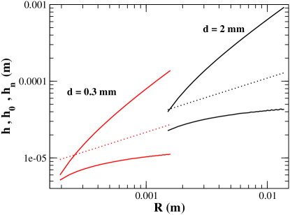
Figure 8: Numerical simulation of Eqs. (15-19). We plot $h_{0}$ and $h_{n}$ (full lines respectively top and bottom) as a function of $R$. The red curve is for $d=0.3$ mm, the black is for $d=2$mm. The dashed-lines represent the scaling $h\propto R^{1/2}$ predicted by Eq. (5) using the data deduced from the experimental measurement of the constant $C$. The prefactor in Eq. 10 are estimated using a best-fit adjustment of the results show on Fig. 3.

III.2 Hole nucleation

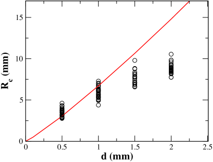
Figure 9: Critical radius $R_{c}$ versus the spacing $d$. Each point corresponds to one experiment. The red line holds for the numerical prediction using Eqs. (15-19)

.

The numerical resolution of the droplet profile as shown in the above section reveals that no solution should exist beyond a critical drop radius $R_{c}$. This statement is thus tested experimentally: we first inject a primary drop in our system that is grown continuously by coalescence with smaller drops. We find that at some point a hole nucleates and grows inside the drops (Fig. 5). The hole grows until it reaches the drop edges. This leads to the destruction of the drop into several fragments that are ejected radially. The critical radius $R_{c}$ exhibits some dispersion, but a clear trend can be observed as a function of the spacing $d$ (Fig. 9). The comparison with the model is rather satisfactory given that there is no free parameter. The agreement is even very good for smaller spacing. For larger spacing we might expect some discrepancies since gravitational effects could play a role as the spacing becomes comparable to the capillary length $l_{c}=\sqrt{\sigma/\rho g}$

IV Oscillation modes

In our experiment, the drops were found to have radial oscillations mode for most of the values of the parameters such as the radius $R$ and the spacing between the two plates $d$. Theses oscillations can be described by star-shaped contour modes with frequencies ranging between 10 and 400 Hz. The modes are thus parametrized by a integer $m$, namely the azimuthal mode number, which measures the number of spikes along the contour of the drop as shown on Fig. 10. As shown for example on Fig. 11, we display the evolution of the droplet for the $m=3$ mode during a half-period, this oscillation is typical of a standing wave pattern.

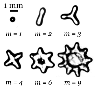
Figure 10: Top views of the droplets. Examples of different oscillation modes. Here $m$ holds for the number of spikes of the drop, $d=1{\rm mm}$ and the horizontal scale is shown by the black bar.

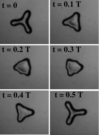
Figure 11: Top view of a single drolet. Time evolution of the $m=3$ mode for a half-period. Here $d=1$ mm, $R=1$ mm and ${\bf{T}}=0.009\,s$.

During a typical experiment in which drops slowly evaporate, we observe that the azimuthal number $m$ has tendency to decrease with time as the drop size decreases. However, there seems to be no stringent dynamics for the time evolution of the azimuthal mode number and in particular a wide range of frequency transitions occurs during the life of a droplet. Furthermore there seems to be no direct link between the azimuthal number $m$ and the droplet radius except for this decreasing tendency. The value of the mode number displays strong stochasticity probably induced by the non-linear coupling between oscillations modes and by the inherent thermal fluctuations which are expected at liquid-vapor interfaces just below the boiling transition.
We plot on Fig. 12 the frequency measurements with respect to the radius $R$ for different values of $m$. They reveal a clear trend well approximated by a power law as explained below. Let us first focus for example on the mode $m=3$ which was observed over the larger range of frequencies and for several values of the spacing $d$. We did not notice any effect of the spacing so that we performed a power law interpolation over all its data. This leads to $f$(Hz)$=(12\pm 1)\times 10^{-4}R$(mm)^-1.7±0.3. Even though other modes $m$ do not span as much frequencies as the mode $m=3$ does, their trends are also compatible with a scaling of $R^{-3/2}$. Such an exponent is therefore reminiscent of the Rayleigh spectrum for capillary wave on spherical drops Lamb1932 or two dimensional discs Takaki1985 for which the frequency also scales likes $R^{-3/2}$ . In order to go deeper in this analysis we have plotted on Fig. 13 the dimensionless frequency $f/f_{0}$ of the contour modes as a function of $m$, where $f_{0}=\frac{1}{2\pi}\sqrt{\frac{\gamma}{\rho R^{3}}}\,.$ is the typical frequency scale. The comparisons between the experimental points and the theoretical results shown on Figure 13 seem to validate the capillary origin of these surface waves. The small discrepancy emphasized by the slight overestimate of the theory may origin from several facts such as the complexity of the Leidenfrost effect which involves vapor flow around the droplet, the possible coupling between the gas dynamics and the fluids at the surface and the particular geometry of a droplet in a Hele-Shaw cell.

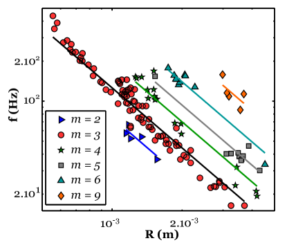
Figure 12: Oscillation frequency $f$ versus the drop radius $R$ in meters. Several modes are represented. Each of them is fitted by a power law with an exponent -3/2 (solid lines). Experiments are performed for $d=1$mm, excepted for $m=3$, where data of $d=0.5$ and 0.3 mm are also plotted.

The comparison of our experimental results with the regular 3D Leidenfrost effect is enlightening. In references Strier2000 , it has been reported that star-like drop shapes can be observed when the droplet is trapped and forced to remain at the same place either by the use of a concave substrate or by the presence of pinning objects such as impurities. Further star-like shapes have also been observed when nitrogen drops are deposited over a viscous liquid at room temperature Snezhko2008 . In this case, the oscillations seem to be coupled to the internal flow inside the drop. More generally the spontaneous oscillation of drop or liquid puddles seems to be more general and has also been observed in other levitated systems without Leidenfrost effect as shown in reference Brunet2011 . In this previous work, a liquid droplet or puddle is levitated over an air cushion which generates a quasi-laminar flow and star-like oscillations are observed Brunet2011 .

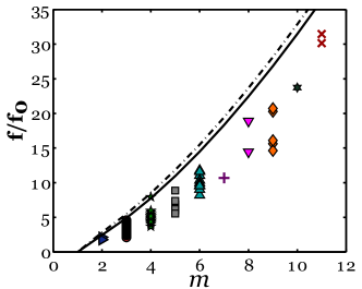
Figure 13: Dimensionless oscillation frequency $f/f_{0}$ vs the mode number $m$. All experiments are plotted ($d=0.3$, 0.5, 1 and 2 mm). For comparison we plot the models of an inviscid 3D spherical drop of the same radius Lamb1932 ($f^{3D}/f_{0}=\sqrt{(m-1)m(m+2)}$, dashed-dotted line) and for a perfectly homogeneous and discoidal 2D puddle Takaki1985 ($f^{2D}/f_{0}=\sqrt{m(m^{2}-1)}$, solid line).

It is noteworthy to mention that in all theses systems (Leidenfrost drops 3d and 2d and levitated air-cushion drop) the relevant frequency of oscillations displays a $R^{-3/2}$ tendency which is a characteristic of Rayleigh capillary wave dispersion relation Snezhko2008 ; BouwhuisPreprint . Here again as for our results (Fig. 13) the measured frequencies seem to be slightly overestimated by the simple capillary wave models Snezhko2008 ; BouwhuisPreprint . This fine difference has not been explained yet to our knowledge and requires as we mention above a mode analysis with the particular geometry.

We also have noticed experimentally (see movie in the supplementary materials) that contour modes seem to be associated with thickness waves in the confined dimension. This could emphasize the occurrence of non-linear coupling between thickness waves and contour waves. Therefore, not only the dispersion relation of the wave shows a small discrepancy as shown in Fig. 13 with the simple models (Rayleigh capilary waves in 2d or 3d) but the origin of the instability leading to star-like droplet still remains unsolved and is of current investigation. For example, the origin of the instability of Leidenfrost puddles in non-confined geometry is still a matter of debate as discussed in reference Brunet2011 . It was proposed that oscillations originate from thermal-convection inside the drop Strier2000 , but observations in athermal systems show that a purely hydrodynamical instability Brunet2011 is the most probable scenario. In the case of air-flow levitated droplet, numerical experiments have been performed and have revealed a possible scenario for the origin of the instability BouwhuisPreprint . In this latter, the hydrodynamical flow inside the drop and inside the sustaining air layer BouwhuisPreprint is numerically investigated and compared to experiments. In both cases, the experiments and numerical simulations exhibit a critical airflow velocity inside the lubricating layer above which the drop begins to oscillate. A mechanism has been postulated where the occurrence of a primary instability (appearance of axi-symetric breathing modes) triggers parametrically a second instability and the appearance of the non-axisymetric contours modes observed experimentally BouwhuisPreprint . For millimeter-sized drops, it was found experimentally that this instability appears for airflow velocities higher than $\sim$ 0.1 m/s . For comparison this value is significantly lower than the airflow values inferred from the evaporation rate in our Leidenfrost Hele-Shaw cell. This could support the hypothesis of purely hydrodynamical instability in our experiments as well.

V Conclusion

We have investigated the behavior of 2d-Leidenfrost droplet in a Hele-Shaw cell. This investigation has revealed a rich behavior of phenomena such has droplet levitation below and above a vapor layer, and the appearance of critical transition from discoidal droplet to torus like droplet. This topological transition occurs due to the thinning of liquid at the center of the droplet. We have characterized experimentally these phenomena and we have presented a theoretical model and a numerical study based on the lubrication approximation which corroborate these experimental facts. We are currently investigating the dynamics of the hole expansion. We also report observations of large amplitude star-like undulation consisting of azimuthal oscillating capillary waves. The frequency of oscillations are measured and are found to be close to the frequency of Rayleigh capillary wave of droplets. Finally, we have discussed possible mechanisms which are at the origin of this instability.

VI acknowledgements

We would like to thank Martine Le Berre and Damien Scandola for fruitful discussions.

VII Appendix A

For the sake of clarity, we derive here Eq. (11). Let us recall that the temperature in the vapor layer is given by

$$T=T_{p}\left(1-\frac{z}{h(x,y)}\right)+T_{b}\frac{z}{h(x,y)}\,.$$ (29)

The horizontal velocity components $u$ and $v$ read using the lubrication approach:

$$u=\frac{z\left(z-h(x,y)\right)}{2\eta}\partial_{x}p\,\,\,{\rm and}\,\,\,v=\frac{z\left(z-h(x,y)\right)}{2\eta}\partial_{y}p\,.$$

Integrating the incompressibility relation:

$$\partial_{x}u+\partial_{y}v+\partial_{z}w=0\,,$$

between $z=0$ where $w=0$ and $z=h(x,y)$ we obtain using Eq. (1),

$$\nabla_{2}\cdot\left(\frac{h^{3}}{12}\nabla_{2}p\right)+\frac{\eta\kappa\Delta T}{h(x,y)}=0\,,$$ (30)

where $\kappa=\lambda/(\rho_{v}L)$   and $\nabla_{2}=\mathbf{e}_{x}\partial_{x}+\mathbf{e}_{y}\partial_{y}$. In cylindrical coordinates, Eq. (30) reads :

$$\partial_{r}\left(\frac{rh^{3}}{12}\partial_{r}p\right)+\frac{r\eta\kappa\Delta T}{h(r)}=0\,.$$ (31)

and is exactly similar to Eq. (11).

References

- (1) J. G. Leidenfrost, “De Aquae Communis Nonnullis Qualitatibus Tractatus”, (Duisbourg, 1756).
- (2) J. D. Bernardin and I. Mudawar, “The Leidenfrost Point: Experimental Study and Assessment of Existing Models”, J. Heat Trans. ASME 121, 894 (1999).
- (3) H. van Dam,“Physics of nuclear reactor safety”, Rep. prog. Phys. 55, 2025 (1992).
- (4) D. Quéré,“Leidenfrost Dynamics”, Ann. Rev. Fluid. Mech. 45, 197 (2013).
- (5) A.-L. Biance, C. Clanet, D. Quéré, “Leidenfrost drops”, Phys. Fluids, 15,1632 (2003).
- (6) F. Celestini, T. Frisch and Y. Pomeau, “Take-off of small Leidenfrost droplets”, Phys. Rev. Lett. 109, 034501 (2012).
- (7) J.C. Burton, A.L. Sharpe, R.C.A. van der Veen, A. Franco and S. R. Nagel, “Geometry of the Vapor Layer Under a Leidenfrost Drop”, Phys. Rev. lett. 109, 074301 (2012).
- (8) F. Celestini and G. Kirstetter, “Effect of the electric field on a Leidenfrost droplet”, Soft Matter 8, 5992 (2012).
- (9) H. Linke, B. J. Aleman, L. D. Melling, M. J. Taormina, M. J. Francis, C. C. Dow-Hygelund, V. Narayanan, R. P. Taylor1, and A. Stout, “Self-Propelled Leidenfrost Droplets”, Phys. Rev. lett. 96, 154502 (2006).
- (10) T. R. Cousins, R. E. Goldstein, J. W. Jaworski and A. I. Pesci, “A ratchet trap for Leidenfrost drops”, J. Fluid. Mech. 696, 215 (2012).
- (11) Y. Pomeau, M. Le Berre, F. Celestini and T. Frisch, “The Leidenfrost effect : From quasi-spherical droplets to puddles”, C. R. Mecanique 340, 867 (2012).
- (12) F. Celestini, T. Frisch and Y. Pomeau, “Room temperature water Leidenfrost droplets”, Soft Matter, 9, 9535 (2013).
- (13) L. Duchemin, J. Lister and U. Lange, “Static shapes of a viscous levitated drop”, Journal of Fluid Mechanics, 533, 161–170 (2005).
- (14) A. Snezhko, E. Ben Jacob and I. S. Aranson, “Pulsating gliding-transition in the dynamics of levitating liquid nitrogen droplets”, New J. Phys. 10, 043034 (2008).
- (15) W. Bouwhuis, K. G. Winkels, I. R. Peters, P. Brunet, D. van der Meer, and J. H. Snoeijer, “Oscillating and star-shaped drops levitated by an airflow”, Phys. Rev E, 88 , 023017-023017 (2013).
- (16) H. Lamb, Hydrodynamics 6th edn. Cambridge University Press, USA (1932).
- (17) L. Rayleigh, On the Capillary Phenomena of Jets Proc. R. Soc. 29, 71–97 (1879). .
- (18) R. Takaki and K. Adachi ,“Vibration of a flattened drop. II- Normal mode analysis”, J. Phys. Soc. Jpn. 54 , 2462–2469 (1985).
- (19) P. Brunet and J. H. Snoeijer, “Star-drops formed by periodic excitation and on an air cushion- A short review”, Eur. Phys. J. Special Topics 192 , 207–226 (2011).
- (20) D. E. Strier, A. A. Duarte, H. Ferrari, G. B. Mindlin, “Nitrogen stars: morphogenesis of a liquid drop”, Physica A 283, 261 (2000).
- (21) P.Tabeling. Introduction to Microfluidics.Oxford University Press. (2005)