3D PROMINENCE-HOSTING MAGNETIC CONFIGURATIONS: CREATING A HELICAL MAGNETIC FLUX ROPE

Abstract

The magnetic configuration hosting prominences and their surrounding coronal structure is a key research topic in solar physics. Recent theoretical and observational studies strongly suggest that a helical magnetic flux rope is an essential ingredient to fulfill most of the theoretical and observational requirements for hosting prominences. To understand flux rope formation details and obtain magnetic configurations suitable for future prominence formation studies, we here report on three-dimensional isothermal magnetohydrodynamic simulations including finite gas pressure and gravity. Starting from a magnetohydrostatic corona with a linear force-free bipolar magnetic field, we follow its evolution when introducing vortex flows around the main polarities and converging flows towards the polarity inversion line near the bottom of the corona. The converging flows bring feet of different loops together at the polarity inversion line and magnetic reconnection and flux cancellation happens. Inflow and outflow signatures of the magnetic reconnection process are identified, and the thereby newly formed helical loops wind around pre-existing ones so that a complete flux rope grows and ascends. When a macroscopic flux rope is formed, we switch off the driving flows and find that the system relaxes to a stable state containing a helical magnetic flux rope embedded in an overlying arcade structure. A major part of the formed flux rope is threaded by dipped field lines which can stably support prominence matter, while the total mass of the flux rope is in the order of 4–5$\times 10^{14}$ g.

1 INTRODUCTION

Observations show that prominences are always residing in the lower regions of coronal cavities, which are tunnel-like regions of reduced electron density along so-called filament channels. When observed at the solar limb, coronal cavities appear as relatively dark, elliptical regions around prominences underneath coronal streamers (Gibson et al., 2010; Waldmeier, 1970). Observations on quiescent prominences suggest that prominences and their surrounding coronal cavities are hosted by a single large-scale structure in the solar corona: a helical magnetic flux rope (Berger, 2012; Wang & Stenborg, 2010). The latest observations of coronal magnetometry on cavities found twist or shear of magnetic field extending up into the cavity and a pattern of concentric rings in line-of-sight velocity which may be explained by a magnetic flux rope model (Bak-Stȩślicka et al., 2013). In situ measurements of interplanetary CMEs showed strong evidence for magnetic flux rope structures (Burlaga et al., 1982), which means that either there is a pre-existing flux rope in a prominence before eruption, or it changes into a flux rope structure during its eruption and propagation. Indications from aligned chromospheric fibrils in filament channels (Foukal, 1971) and from direct measurements of prominence magnetic fields (Leroy et al., 1983) show that the magnetic field in a filament channel has a strong component along the direction of the polarity inversion line (PIL), which is consistent with a weakly twisted flux rope model. Magnetohydrostatic solutions for the support of prominence matter within a 2.5D flux rope have been presented in analytical (Low & Zhang, 2004) and numerical (Blokland & Keppens, 2011; Hillier & van Ballegooijen, 2013) models. Therefore, a helical magnetic flux rope is a promising magnetic structure to host a prominence.

The origin of a magnetic flux rope in the corona has been explained by two theories: (1) a pre-existing flux rope in the convection zone emerges through the solar surface into the corona near active regions (Okamoto et al., 2008; Fan, 2001, 2010); (2) magnetic reconnection and flux cancellation at the PIL of a sheared magnetic arcade leads to the formation of helical field lines (van Ballegooijen & Martens, 1989; Martens & Zwaan, 2001). From observations, Mackay et al. (2008) found that most filaments are outside of active regions and their formation is not directly related to flux emergence but results from flux cancellation or coronal reconnection. Observations indicate that flux cancellation, which is the mutual disappearance of positive and negative magnetic flux when they encounter each other at PILs in photospheric magnetograms, constantly happens during the formation of a filament (Wang & Muglach, 2007; Chae et al., 2001). Theoretical considerations (van Ballegooijen & Martens, 1990) and 2.5D numerical studies creating force-free magnetic field configurations for flux ropes embedded in arcades (van Ballegooijen & Martens, 1989) suggested that photospheric mass flows may cause restructuring of coronal magnetic fields, leading to flux rope formation and eruption. Two kinds of photospheric flows have been considered as the main driver: shear flow and converging flow. Shear flow caused by flux emergence, differential rotation, meridional flow, and magnetic diffusion stretches coronal field arcades creating an axial component of the magnetic field. Net converging flows toward the PIL in weak field regions is the result of magnetic elements diffusion caused by random supergranular motions, which tend to transport radial magnetic flux from regions of high flux density to regions of low flux density (Zirker et al., 1997; Leighton, 1964). Converging flows bring opposite-polarity magnetic elements, which are feet of different magnetic loops, to collide at the PIL. This drives photospheric magnetic reconnection (Litvinenko et al., 2007) (causing the flux cancellation phenomenon) to effectively change the topology of magnetic field from arcades into helical flux ropes and increases the axial component magnetic field.

Based on the flux cancellation mechanism, many numerical models (e.g. Amari et al., 1999, 2000, 2003a, 2003b, 2010; Mackay & van Ballegooijen, 2006; Yeates & Mackay, 2009) have produced twisted flux ropes. They use different driving means applied as bottom boundary condition, such as (1) imposing a time-dependent decrease of the magnetic flux via prescribed electric fields; (2) imposing time-dependent vertical magnetic fields derived from large-scale photospheric motions such as differential rotation, meridional flow, and surface diffusion; and (3) imposing shearing flows or converging flows at the PIL via prescribed velocity fields. Most of these models were solving simplified magnetohydrodynamic (MHD) equations. In particular, nonlinear force-free (magnetic field only) configurations were used in Mackay & van Ballegooijen (2006); Yeates & Mackay (2009) to adress the evolution of large-scale to global coronal field solutions due to photospheric flux changes. A frequently made assumption is to work in zero-$\beta$ conditions, excluding gas pressure and neglecting solar gravity (Amari et al., 1999, 2000, 2003a, 2003b, 2010; Lionello et al., 2002), while a (topologically oriented) comparison between zero-$\beta$ MHD and nonlinear force-free models for a sigmoidal flux rope is found in (Savcheva et al., 2012). However, the overall equilibrium balance, plasma thermal structure, and small-scale dynamics of quiescent prominences may be significantly affected by gas pressure and gravity. Selected global models (Linker et al., 2001, 2003) did include gravity and finite beta effects, using typically polytropic MHD assumptions (with polytropic indices mimicking near isothermal conditions) in 3D, while full thermodynamic effects have only entered reduced dimensionality simulations (Linker et al., 2001; Lionello et al., 2002). These works usually focus on (loss of) global equilibrium and the eruption of prominences, while we will concentrate on a local, 3D isothermal model addressing details of flux rope formation with a stable flux rope endstate suitable for prominence support. Some ideal MHD simulations at finite beta but without gravity included produced twisted field lines from arched loops by coronal reconnection driven by shearing flows or converging flows at the bottom (DeVore & Antiochos, 2000; DeVore et al., 2005; Welsch et al., 2005). But the final assembly of those twisted field lines did not resemble typical flux ropes with elliptical cross-sections, an aspect which we will demonstrate here, while including gravity.

In this paper, we perform 3D isothermal MHD numerical simulations, at realistic finite-$\beta$ regimes in a gravitationally stratified solar coronal atmosphere. Our aim is to generate a helical flux rope self-consistently starting from a simple arcade configuration by imposing systematic photospheric motions. The first step is to build a sheared magnetic arcade field, using extrapolation techniques, augmented with a stratified atmosphere. The second step will introduce converging photospheric flows that drive magnetic reconnection along the PIL. This is here achieved in finite-$\beta$ MHD, realizing an endstate that relaxes to a stable flux rope which can host a prominence. This paper is structured as follows. In Section 2 we describe the numerical method and the modeling procedure. The results and analysis are gathered in Section 3. A general description of the flux rope formation process is given in Subsection 3.1. Subsection 3.2 reports the analysis of the magnetic reconnection that gives birth to the large-scale helical flux tubes. Force analysis and twist property are given in Subsection 3.3 and Subsection 3.4 respectively. Conclusions and an outlook are given in section 4.

2 NUMERICAL METHOD

2.1 Initial setup and governing equations

The computational domain is a 3D finite box of sizes $-120<x<120$ Mm, $-90<y<90$ Mm, and $3<z<123$ Mm in Cartesian coordinates, intended to be large enough to cover the coronal part of a complete filament channel. We first set up an initial magnetic field by linear force-free field extrapolation from an analytic, bipolar magnetogram $B_{m}=B_{z}(x,y,z=0,t=0)$ with the magnetic field strength range in $\pm 20$ G at the height of $z=0$ Mm. $B_{m}$ is composed of two elliptic Gaussian distributions placed across the $x$-axis (the PIL is in the $x$-direction):

$$B_{m}=B_{0}\exp(-\frac{(x-x_{1})^{2}}{2\delta x^{2}}-\frac{(y-y_{1})^{2}}{2\delta y^{2}})-B_{0}\exp(-\frac{(x-x_{2})^{2}}{2\delta x^{2}}-\frac{(y-y_{2})^{2}}{2\delta y^{2}}),$$ (1)

where $B_{0}=20$ G, $x_{1}=x_{2}=0$ Mm, $y_{1}=-y_{2}=40$ Mm, $\delta x=50$ Mm, and $\delta y=20$ Mm. We use this magnetogram prescription to construct a first 3D linear force-free field in the entire box. The linear force-free field is integrated by the exact Green’s function method (Chiu & Hilton, 1977) with constant $\alpha=-0.08$. Because the pressure scale height in the lower corona is relatively large, we simplify the thermodynamics to an isothermal assumption, taking the uniform temperature fixed at $T_{0}=1$ MK. We then still need to prescribe a pressure-density variation throughout the box, but from hydrostatic equilibrium under gravitational stratification, the density distribution is derived to be

$$\rho=\rho_{b}\exp[-\frac{g_{\odot}r_{\odot}^{2}}{RT_{0}}(\frac{1}{r_{\odot}}-\frac{1}{r_{\odot}+z})]\,$$ (2)

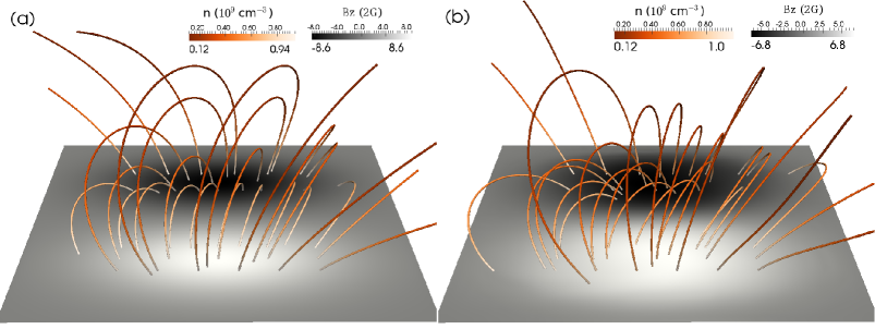
Figure 1: (a) Initial linear force-free field as a sheared arcade extrapolated from the bottom magnetogram $B_{z}$ in a gray scale; (b) more realistic arcade after twisting motion driven at the bottom. Magnetic field lines in orange and white are colored by the number density of plasma. The color bars are scaled to the instantaneous data range. (A color version of this figure is available in the online journal.)

with $\rho_{b}=2.34\times 10^{-15}$ g cm^-3 the bottom density at $z=0$, $g_{\odot}$ the solar surface gravitational acceleration, $r_{\odot}$ the solar radius, and gas constant $R$. The gas pressure is finite and follows the ideal gas law $p=\rho RT_{0}$. There is no flow prescribed initially. This initial magnetic configuration, along with information on the density structuring is shown in Figure 1(a).

In all subsequent steps, we proceed by solving the isothermal MHD equations given by

$$\frac{\partial\rho}{\partial t}+\nabla\cdot\left(\rho\mathbf{v}\right) =0,$$ (3)

$$\frac{\partial\left(\rho\mathbf{v}\right)}{\partial t}+\nabla\cdot\left(\rho\mathbf{vv}+p_{\rm tot}\mathbf{I}-\frac{\mathbf{BB}}{\mu_{0}}\right) =\rho\mathbf{g}-\nabla\cdot\Pi,$$ (4)

$$\frac{\partial\mathbf{B}}{\partial t}+\nabla\cdot\left(\mathbf{vB}-\mathbf{Bv}\right) =0,$$ (5)

where $\rho$, $\mathbf{v}$, $\mathbf{B}$, and $\mathbf{I}$ are the plasma density, velocity, magnetic field, and unit tensor, respectively, while the total pressure is $p_{\rm tot}\equiv p+\frac{B^{2}}{2\mu_{0}}$ and $\mathbf{g}=-g_{\odot}r_{\odot}^{2}/(r_{\odot}+z)^{2}\mathbf{\hat{z}}$ is the gravitational acceleration with $r_{\odot}$ the solar radius and $g_{\odot}$ the solar surface gravitational acceleration. The mass conservation equation and ideal MHD induction equation are augmented with a momentum equation where we incorporate a stress tensor $\Pi$ having components $\Pi_{ij}=-\mu\left(\frac{\partial v_{i}}{\partial x_{j}}+\frac{\partial v_{j}}{\partial x_{i}}-\frac{2}{3}\delta_{ij}\nabla\cdot\mathbf{v}\right)$ with the dynamic viscosity coefficient $\mu=0.5$ g cm^-1 s^-1 and the Kronecker delta $\delta_{ij}$. For the normalization of the equations, we set the unit of length, number density, velocity, and magnetic field to be 10 Mm, $10^{9}$ cm^-3, 116.45 km/s, and 2 G respectively. We use the parallelized Adaptive Mesh Refinement (AMR) Versatile Advection Code (MPI-AMRVAC; Keppens et al., 2012) to numerically solve these equations. We choose a third-order accurate, shock-capturing scheme combining an HLL(C) scheme (Mignone & Bodo, 2006) and a third order Cada-limited reconstruction, with a three-step Runge-Kutta time marching (Čada & Torrilhon, 2009). The constraint $\nabla\cdot\mathbf{B}=0$ is controlled by a diffusive approach, which diffuses away any numerically generated divergence of magnetic field at the maximal rate allowed by the CFL condition (van der Holst & Keppens, 2007; Keppens et al., 2003). In practice, the magnetic field then gets updated according to $\mathbf{B}+C_{d}\left(1/\Delta x^{2}+1/\Delta y^{2}+1/\Delta z^{2}\right)^{-1}\nabla\nabla\cdot\mathbf{B}$ where we take $C_{d}$ of order unity while using centered differencing approximations for the gradients. The AMR grid we use has three levels and an effective resolution of $512\times 384\times 256$ with spatial resolving ability of 469 km. The automated refining (or coarsening) decisions are made upon the local error estimation of magnetic field and density with 90% and 10% weights respectively. The Level 1, Level 2, and Level 3 grids cover 74%, 13.4%, and 12.6% of the total volume of the box respectively.

2.2 Twisting the arcade system

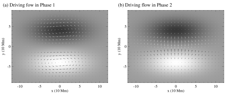
Figure 2: (a) twisting and (b) converging velocity field (shown by arrows) on top of the magnetogram in a gray scale on the bottom boundary in Phase 1 and Phase 2 respectively.

By construction, the initial magnetic arcade is non-potential but linear force-free and the topology is such that the larger magnetic loops connecting the outer regions in arch-shaped field lines have larger shearing angles relative to the PIL than the smaller loops connecting opposite polarities near the central PIL. This can be seen in the field lines as shown in Figure 1(a). However observations typically show that the larger/higher magnetic loops are more close to potential fields, and in particular exhibit smaller shearing angles than the underlying smaller loops (Martin, 1998). To adjust the arcade to this more realistic topology, we impose a horizontal twisting velocity field on the bottom boundary, which is composed of two large-scale in-plane vortices rotating in the same direction around the two main polarities (see Figure 2(a)), such that the vertical component of the magnetic field at the bottom is preserved (Amari et al., 1996). This twisting flow is not intended to model real flows on the sun. The twisting velocity field is formulated as

$$v_{x}^{a}=f(t)\frac{\partial\phi}{\partial y},~{}~{}~{}~{}v_{y}^{a}=-f(t)\frac{\partial\phi}{\partial x},~{}~{}~{}~{}\phi=C_{0}B_{m}^{2}\exp(\frac{B_{m}^{2}-B_{max}^{2}}{\delta B^{2}}),$$ (6)

where $B_{max}\approx 20$G is the maximum value of $B_{m}$, $\delta B=5B_{max}$, $f(t)$ is a linear ramp function with values between 0 and 1 to switch the driving smoothly on and off with a ramp of 14.3 min, and the amplitude factor $C_{0}$ is chosen so that the imposed velocity magnitude has a maximum value of 11.8 km s^-1 and the maximum initial Alfvén Mach number is 0.0126. Note that the driving velocity prescription is used to fill the cell-centered velocities in the ghost cells of the bottom boundary. In doing so, the velocity on the bottom plane, which corresponds to a cell face, can still adopt some intermediate value between the first physical cell-center value and the imposed ghost cell-center value. This local bottom plane value is computed during the (nonlinear) cell-center to cell-edge limited reconstruction procedure and next applied in the flux quantifications. This means that fluxes at the bottom boundary plane may not be zero when the driving flow is switched off, as we will see later. We then time advance the isothermal MHD equations from above, augmented with further boundary prescriptions. We impose zero vertical velocity on the bottom face and zero velocity on the other five faces of the box during this phase by antisymmetric boundary condition. For the boundary condition of the magnetic field, we do extrapolation keeping the normal gradient to be zero. The scheme is one-sided third-order accurate finite difference for the bottom and second order for the other faces. Then we modify the normal component to fulfill the divergence-free condition discretely using a second-order centered difference evaluation. We use zeroth order extrapolation for the density on side boundaries, fixed gravitationally stratified density at the bottom, and adopt a gravitationally stratified density profile at the top extrapolated by second order centered difference. The twisting driving velocity imposed at the bottom boundary lasts for 43 minutes or 54 $\tau_{\rm A}$ (using the average Alfvén time scale $\tau_{\rm A}=$48 s) including two linear ramps of 14.3 min each to switch this twisting motion on and off. Then the system evolves in a viscous relaxation for another 43 minutes to reach a quasi-static state where the lower smaller loops are further sheared while the overlying larger loops become closer to potential field, as shown in Figure 1(b). The time evolution of the kinetic energy $E_{K}$ and the magnetic energy $E_{B}$ of the whole system during this phase is shown in Figure 3(a). In order to understand the temporal evolution of $E_{B}$, we quantify its time derivative, and compare it to the total net Poynting flux through the six faces of the box, and the power of the Lorentz force in the full domain. These correspond to the first, second, and third term in the following formula derived from the conservation law of magnetic flux as

$$\frac{\partial}{\partial t}\int_{V}\frac{B^{2}}{2\mu_{0}}dV=-\int_{S}\frac{1}{\mu_{0}}\mathbf{B}\times(\mathbf{v}\times\mathbf{B})\cdot d\mathbf{S}-\int_{V}(\mathbf{J}\times\mathbf{B})\cdot\mathbf{v}dV$$ (7)

where $V$ is the total volume of the 3D box with its six faces represented by $\mathbf{S}$. The quantities of these terms versus time are plotted as the dotted line, the dashed line, and the solid line in Figure 3(c), respectively. The temporal change of $E_{B}$ is dominated by the Poynting flux caused by the horizontal flows on the bottom face, while the magnitude of the Lorentz force power is about 50 times smaller than the Poynting flux. The twisting driving flows inject kinetic energy and magnetic energy into the domain. After the driving stops, the twisted magnetic arcade tends to relax, inducing a reverse rotating motion on the bottom face which emits away magnetic energy via the Poynting flux. This is, as mentioned before, a consequence of our use of ghost cell-center prescriptions to (indirectly) impose fluxes through this face, rather than work with a discretization which directly controls the face flux. Due to viscous dissipation, the kinetic energy drops quickly when the driving flows start to decrease and in the end relaxes to a very small value with a maximal speed remnant of 3.8 km s^-1. The ratio of the electric current that is perpendicular to the magnetic field over the total electric current in a volume $\mathcal{V}$:

$$\sigma_{\mathbf{J}}\equiv=\frac{\int_{\mathcal{V}}|\mathbf{J}_{\perp}|d\mathcal{V}}{\int_{\mathcal{V}}|\mathbf{J}|d\mathcal{V}}=\frac{\int_{\mathcal{V}}|\mathbf{J}\times\mathbf{B}|/|\mathbf{B}|d\mathcal{V}}{\int_{\mathcal{V}}|\mathbf{J}|d\mathcal{V}}$$ (8)

is a common measure of the degree of force-freeness of magnetic field in the volume $\mathcal{V}$ (Valori et al., 2012). At the end of this phase, $\sigma_{\mathbf{J}}$ is 0.055 while at the initial state it is 0.021. For a magnetic field that is ideally force-free, $\sigma_{\mathbf{J}}$ equals zero.

2.3 Converging flows prescription

From the end state of the first phase, we start the second phase by imposing a converging velocity field toward the PIL ($y=0$) on the bottom boundary filling bottom ghost cell layers with the horizontal velocity formulated as

$$v_{x}^{b}=-f(t)C_{1}\frac{\partial|B_{m}|}{\partial x}\exp(-y^{2}/y_{d}^{2}),~{}~{}~{}~{}v_{y}^{b}=-f(t)C_{1}\frac{\partial|B_{m}|}{\partial y}\exp(-y^{2}/y_{d}^{2}),$$ (9)

where $y_{d}=50$ Mm quantifies an additional Gaussian width parameter away from the PIL, $f(t)$ is a linear ramp function as in equation (6), and the amplitude factor $C_{1}$ is chosen so that the driven speed has a maximum value of 12.3 km s^-1 and the maximum initial Alfvén Mach number is 0.0216. The pattern of the converging flows is time independent, since $f(t)$ contains the only time-dependent part. Net converging flows towards the PIL in weak field regions are an effective result of magnetic elements diffusion caused by random supergranular motions. These tend to transport vertical magnetic flux from regions of high flux density to regions of low flux density (Zirker et al., 1997; Leighton, 1964). Figure 2(b) shows this imposed velocity field by arrows on top of the magnetogram $B_{m}$. We then once more simulate the isothermal MHD equations forward in time. During this phase, we keep $\mathbf{v}=\mathbf{0}$ at the four side boundaries, and use a limited open boundary condition at the top and bottom boundaries to allow both upward and downward flows to pass through the boundaries. This is achieved as follows. First, we extrapolate the normal velocity ensuring zero normal gradient across the boundary by one-sided 3rd-order finite differences. Then, the normal velocities on the bottom and the top boundary are clipped to never exceed an upper limit of 10% of the local Alfvén speed to prevent destabilisation by possible high speed flows near boundaries. The speed of pure downflows at the bottom is further limited to not be faster than 1% of the local Alfvén speed. Hence at the bottom near the PIL, induced vertical flows are allowed, but will preferentially go upwards. Note that these induced flows can match or even exceed the imposed horizontal driving velocity magnitude. The density on the bottom boundary is extrapolated by gravitational stratification and kept no less than its initial value. The density on the other boundaries and the magnetic field prescriptions on all boundaries are set up in the same way as in the first phase. The converging motion drives the system for 50 minutes including linear on-off ramping phases. Note that the velocity on the bottom face is not imposed to be zero after the driving flow stops. The time evolution of the kinetic energy and the magnetic energy of the whole system during this phase is plotted in Figure 3(b). Similar to phase 1, we plot also the time derivative of $E_{B}$, the Poynting flux through the six faces of the box, and the power delivered by the Lorentz force versus time during this phase in Figure 3(d). In the first 20 min, the Poynting flux induced by the converging flow dominates and carries away magnetic energy through the bottom. Later, the reconnection-induced upflows, lifting strong horizontal field near the PIL, dominates the Poynting flux which injects magnetic energy into the box. After the horizontal driving flow stops, weak upflows along the PIL keep pumping magnetic energy into the box, while the system slowly relaxes to a more stable state. In the end, the maximal speed remnant is 33 km s^-1 near the top boundary. It is during this phase that we witness the formation of a large-scale flux rope structure, and its eventual relaxation to a stable configuration as described in the following sections.

3 RESULTS

3.1 Birth of A Flux Rope

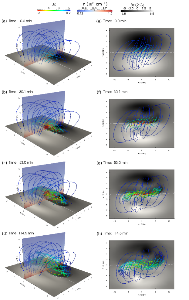
Figure 4: Snapshots of the flux rope formation process at time 0 (first row), 30.1 (second row), 53 (third row), and 114.5 (bottom row) minutes. The bottom magnetograms are shown in gray with the PIL plotted in white. Magnetic field lines are colored by $x$-component of the local current density $J_{x}$ in the rainbow color table. The translucent vertical planes are colored by number density in the blue-red color table. Side views and top views are shown in the left and right column respectively. (A color version of this figure is available in the online journal.)

As the converging flows in frozen-in conditions force the footpoints of magnetic loops to approach the central PIL, the loops get sheared even further. This is seen in Figure 4(a)–(b). By construction, the loops most efficiently affected by the converging flows are rooted in the regions closer to the PIL, while loops rooted near the polarity centers or further away from the PIL are roughly unchanged, as can be seen in Figure 4(e)–(h). In the regions near the PIL, more and more magnetic flux of the loops is transferred to the direction parallel to the PIL. This is consistent with acquired knowledge from observations, stating that before the appearance of a filament near active regions, H$\alpha$ fibril structures (likely tracing the local magnetic field lines) change their orientation from nearly perpendicular to nearly parallel to the PIL (Wang & Muglach, 2007). As the footpoints rooted in flux elements of opposite polarities are forced to collide at the PIL, magnetic reconnection happens there. As a result of the magnetic reconnection near their footpoints, pairs of arched magnetic flux tubes originally separate in $x$-extension now become linked together in a head-tail style, producing a long helical flux tube represented by the red central field line in Figure  4(b)(f). It is to be noted that our ideal MHD run leaves the reconnection process to the inherent numerical diffusion in the employed numerical discretization. We will however provide evidence for the physical correctness of its manifestation in the next section. This newborn helical flux tube has a centrally concave magnetic dip, and hence ascends due to magnetic tension, while the magnetic reconnection below it continues to generate new helical flux tubes. These new helical flux tubes form and wrap around prior-formed ones and together they assemble into a large scale helical flux rope, which rises, expands, and stretches overlying loops.

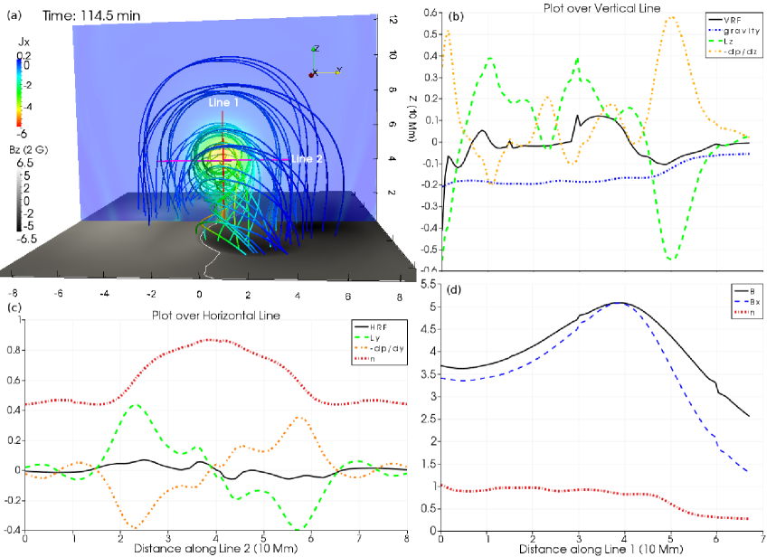
Figure 7: Analysis of the end state at time 114.5 min. (a) a view through the axis of the flux rope with field lines as well as the vertical cutting plane colored by $J_{x}$; (b) distributions of gravity (blue dotted line), vertical Lorentz force (green dashed line), vertical pressure gradient force (orange dotted line), and vertical resultant force (black line) along Line 1 shown in panel (a); (c) distributions of number density (red dotted line), horizontal Lorentz force (green dashed line), horizontal pressure gradient force (orange dotted line), and horizontal resultant force (black line) along Line 2 in panel (a); (d) distributions of magnetic field strength (black line), $x$-component of magnetic field (blue dashed line), and number density (red dotted line) along Line 1 shown in panel (a). The line plot vertical ranges use dimensionless values with these units: $3.2\times 10^{-10}$ dyne cm^-3 for forces, $10^{9}$ cm^-3 for number density, and 2 Gauss for magnetic field. (A color version of this figure is available in the online journal.)

A translucent vertical slice ($oyz$ plane), perpendicular to the $x$-axis, cuts through the center of the box in each panel of Figure 4(a)–(d) and it is colored by the local density. We define the axis of the flux rope by a central magnetic field line on which the poloidal magnetic field vanishes. Since the flux rope perpendicularly goes through the vertical slice, the poloidal magnetic field in the plane can be approximately quantified by $B_{pol}=\sqrt{B_{y}^{2}+B_{z}^{2}}$. The axis of the flux rope intersects the plane at the point where $B_{pol}$ takes the smallest value. In practice, the position of this point is approximately represented by the midpoint position of the grid cell where $B_{pol}$ reaches the smallest value in the plane. We plot the height of this point and the local vertical plasma velocity there versus time to represent the evolution of the axis in Figure 5. Note that the plot starts from time $t=$28.6 min, since before this time the axis of the flux rope can hardly be identified with sufficient resolution. From time 28.6 minutes until the driving flows cease at time 50 min, the average ascending speed of the axis of the flux rope is about 13.3 km s^-1 which is close to the bottom driving speed. Since the ascending magnetic dips also carry along denser plasma upwards from lower altitude, the density inside the flux rope structure ends up to be higher than its surroundings, as shown by the density distribution in the translucent vertical slices in Figure 4(b)–(d). After ceasing the converging driving flows at time 50 min, the flux rope first still continues to rise and expand (see Figure 4(c)–(d)&(g)–(h) and Figure 5). The strong current along the axis of the flux rope is attenuated in this expansion phase. At the end of the run at time 114.5 min, the system reaches a stable state, as will be demonstrated further on by quantifying the force balance. Moreover, when we continue the run to time 150 min, the height of the flux rope axis does not change anymore beyond time 103 min and the local speed on axis is nearly zero (see Figure 5, the remnant velocities cause minor displacements that remain within the local grid cell further on). The vertical cross section of this mature flux rope is roughly elliptic rather than circular, as shown by the vertical slice of density in Figure 4(d) and more clear in the slice of $x$-component current density in Figure 7(a). The vertical extension of the central part of the flux rope ranges from 14 Mm to 60 Mm, and the horizontal extension perpendicular to its axis is about 40 Mm. The ratio of the horizontal extension over the vertical one in the flux rope central cross section is 0.87. This elliptic shape of the flux rope cross-section is consistent with the elliptic shape often observed of coronal cavities (Forland et al., 2011), and aided by incorporating gravity which was ignored in earlier zero-$\beta$ flux rope formation studies (Amari et al., 1999). To estimate the volume and the mass that the flux rope contains, we empirically find that the regions where the absolute value of $B_{x}J_{x}$, i.e. the product of the $x$-component magnetic field and of current, goes over a threshold of $3.18\times 10^{-10}$ dyne cm^-3 roughly fill the volume of the flux rope. The estimated volume and the mass is in the ranges of $2.3$–$3.2\times 10^{29}$ cm³ and 4–$5\times 10^{14}$ g respectively. The mass of a prominence estimated by observations (Gilbert et al., 2011) is in the range of $1.04\times 10^{13}$–$2.14\times 10^{14}$ g which is less than the mass of our flux rope. Roughly half the volume of our flux rope is threaded by dipped field lines that can gather and stably support prominence mass in their magnetic dips, so the mass in those dipped field lines is still significant compared to the mass of a prominence. Moreover, it has been shown that the thermal instability can induce catastrophic cooling to form prominence condensations along field lines (Xia et al., 2011, 2012), but this requires full energetic processes to be simulated.

3.2 Details of Magnetic Reconnection

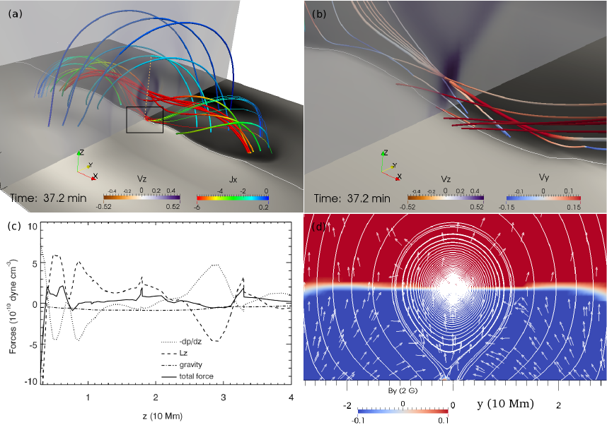
Figure 6: Magnetic reconnection near the PIL at time 37.2 minutes. (a) Overview of the large-scale flux rope colored by $J_{x}$ in rainbow color table with vertical translucent plane colored by vertical velocity $V_{z}$ in brown-purple color table; (b) Zoom-in view of the reconnection site delimited by the black rectangle in (a), where the field lines are now colored by $V_{y}$ in a blue-red color table; (c) Distributions of vertical forces, such as Lorentz force L_z (dashed line), pressure gradient force (dotted line), gravity (dash dotted line), and the total force (solid line), along the vertical yellow dotted line in (a); (d) Poloidal magnetic field lines and arrows of flow directions on top of the vertical plane $oyz$ which is colored by $y$-component magnetic field saturated between $\pm 0.2$ Gauss. Velocity values are dimensionless with a unit of 116.45 km s^-1. (A color version of this figure is available in the online journal.)

To find evidence in favor of magnetic reconnection, we investigate the system in detail at time 37.2 min when the converging flows are still ongoing. As shown in Figure 6(a), the growing flux rope and its overarching arcade are clearly identifiable and indicated by representative field lines colored by $J_{x}$ in a rainbow color table. The vertical translucent plane in this figure where vertical velocities are quantified is cutting through the flux rope, and shows that the highest ascending speed regions locate in the outer layers of the flux rope and near but above the bottom surface along the PIL. We also plot some field lines threading through a site of magnetic reconnection at the PIL. To show these field lines clearly, a zoom-in view of the region in the black rectangle in Figure 6(a) is plotted at right in Figure 6(b). There, the field lines are colored by the $y$-component of velocities $V_{y}$ in a blue-red color table. The red field line sections move in the positive $y$-direction and the blue in the negative $y$-direction. This allows us to identify that field lines from different polarities are approaching each other, leading to magnetic reconnection at intersections near the PIL. These field lines are clearly driven towards each other by flows speeds of 18–23 km s^-1, which exceed the local driving speed (about 12 km s^-1) at the bottom surface. The end result causes topological changes in the field line patterns fully consistent with ongoing magnetic reconnection. In Figure 6(b), the thick field line represents a newly reconnected helical magnetic field line that joins in the flux rope as its outermost layer. We cut a vertical slice through the central part of the flux rope in Figure 6(d) which shows the poloidal magnetic field lines, velocity arrows, and $y$-component of magnetic field in blue-red colors saturated at $\pm 0.2$ Gauss. The concentric ellipses of poloidal field line show the cross section of the flux rope where the outer layer has a tear-drop shape with a cusp reaching down close to the bottom. Under the cusp, the $y$-component magnetic field changes sign indicating a small arcade and a X-point between them. The axis of the flux rope goes through the center of the concentric ellipses, at which height the y-component magnetic field changes sign. The randomly located arrows show directions of the local velocity in the plane. The interpretation is that as the flux rope is rising, the plasma at lower corona outside the flux rope is moving toward it driven by the bottom converging motion and sucked into the X-point. To understand the dynamics, we plot in Figure 6(c) the vertical force distribution at this time along the yellow dotted line in Figure  6(a). The Lorentz force and pressure gradient force oppose each other and vary significantly at different heights. Below 3.7 Mm a strong downward Lorentz force dominates due to the magnetic tension in the concave down small loops. Above a height of 4 Mm up to 25 Mm inside the flux rope, the Lorentz force is upward, as well as the total force, which leads to creating newborn flux tubes and also their ascending in the flux rope as shown by the vertical velocity distribution in purple in the vertical plane. The strongest upflows (up to 60 km s^-1) appear just above the sites of magnetic reconnection. The gravity is relatively small and dynamically only enhanced a little inside the flux rope due to the density enhancement there. From 25 Mm to 31.5 Mm the Lorentz force is downward again, which means that the ascending flux rope is ultimately restrained by the overlying magnetic arcade. Since we are limited to an isothermal model, the thermal energy release of magnetic reconnection is not captured, but the conservative nature of the numerical scheme ensures overall mass, momentum and magnetic flux evolutions consistent with the (partially open) boundary prescriptions, while the energy evolution is constrained to yield an isothermal endstate.

3.3 Overall Force Balance

To understand the stability of the flux rope at the end of the simulation, we quantify the forces along two lines, vertical Line 1 and horizontal Line 2, which go across the central part of the flux rope as shown in Figure 7(a). In the vertical direction, the gravity, Lorentz force, the pressure gradient force, and the vertical resultant force (VRF) are quantified along Line 1 shown by Figure 7(b). The Lorentz force and the pressure gradient force fluctuate and oppose each other. Combined with gravity, the VRF is roughly around zero, which means the flux rope is overall stabilized vertically. Strong negative (downward) Lorentz force and the VRF near the very bottom are results of the magnetic striction of low-lying small arcades under the flux rope. In the upper layer of the flux rope, downward Lorentz force tends to hold down the inflating flux rope. In the rest part, the positive (upward) Lorentz force shows a lifting tend and is compensated by the gravity and gas pressure effect. The distributions of total magnetic field strength, $x$-component magnetic field, and the number density are shown in Figure 7(d). The number density deviates from the hydrostatic state with an enhancement inside the flux rope, and so does the influence of gravity. The magnetic field strength is enhanced inside the flux rope and reaches its maximum at the axis of the flux rope, where the poloidal magnetic field is zero ($B=B_{x}$). In the horizontal direction along Line 2, the Lorentz force in the flux rope, which points to the center from two sides , is almost compensated by the gas pressure gradient force pointing outward from the center. The horizontal resultant force (HRF) is nearly zero showing a force balance in the horizontal direction. The number density inside the flux rope is enhanced and reaches the maximum (2 times denser than the same altitude outside the flux rope) at the center. The flux rope is self pinching and resisted by gas pressure. Thus the enhancement of the density inside the flux rope has two reasons: (1) higher density plasma from lower atmosphere being brought up, (2) squeezing effect by the Lorentz force on the flux rope. The degree of force-freeness of the magnetic field in the computational box now is 0.086, increased by 56% from the beginning state of the second phase. The magnetic field of the system deviates further away from force-free field.

3.4 Twist of the Flux Rope

To quantify the helical property of the flux rope and to check whether the kink instability might happen, we compute the twist of the flux rope. The twist density (in the unit of turns) of a curve $\mathbf{B}$ around a smooth axis curve $\mathbf{A}$ is defined as

$$\frac{d\phi}{ds}=\frac{1}{2\pi}\mathbf{T}(s)\cdot\left(\mathbf{V}(s)\times\frac{d\mathbf{V}(s)}{ds}\right)$$ (10)

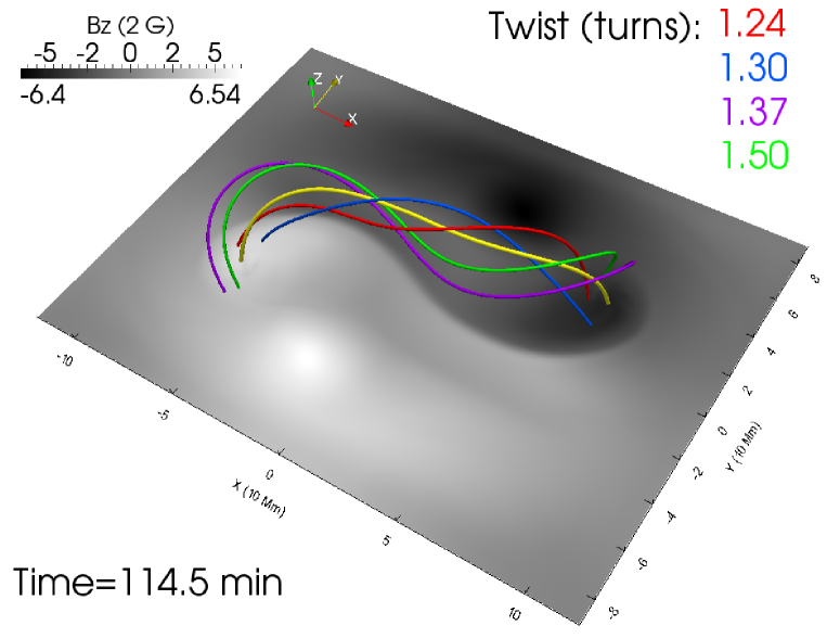
Figure 8: The twists (in turns) of four field lines of the flux rope winding around the axis field line (yellow line) are 1.24 (red line), 1.30 (blue line), 1.37 (purple line), and 1.50 (green line) at the time 114.5 min. (A color version of this figure is available in the online journal.)

where $s$ is the distance along the axis curve, $\mathbf{T}(s)$ is a tangential unit vector of $\mathbf{A}$, and $\mathbf{V}(s)$ is a unit vector normal to $\mathbf{T}(s)$ and pointing from the point $\mathbf{A}(s)$ to a point on $\mathbf{B}$ (Guo et al., 2010; Berger & Prior, 2006). The integration of this equation along the axis curve $\mathbf{A}$ gives the twist of the curve $\mathbf{B}$. We select few representative magnetic field lines that wind the axis of the flux rope in the flux rope, and compute their twists. The result is shown in Figure 8. The average twist 1.35 is smaller than the lower limits of the twist for kink-unstable coronal flux ropes of 1.5 and 1.75 turns found by Fan & Gibson (2003) and Török et al. (2004), respectively. So our flux rope is kink-stable. In the middle of the flux rope, the field lines that go above the axis have smaller twist than the field lines that pass it from below.

4 CONCLUSIONS AND DISCUSSION

We reported on the self-consistent formation of a 3D stable, large-scale, plasma carrying flux rope by successive footpoint shearing and converging flows, followed by relaxations towards near-perfect force-balanced endstates. We quantitatively analyzed the evolution of the magnetic energy, the degree of non force-freeness in the flux rope, the accumulated mass, and its most important geometric features. Improvements to previous efforts are the combination of (1) the gravitationally stratified atmosphere incorporated at finite $\beta$; (2) the elliptic cross-sectional flux rope shape in agreement with recent observations; (3) the equilibrium balance between pressure gradient, Lorentz force and gravity as demonstrated in the endstate; and (4) the fact that a kink-stable flux rope persists on a long timescale, itself trapping sufficient plasma to potentially condense into a true prominence within the flux rope. The latter aspect can only be demonstrated fully when relaxing the assumption of isothermal conditions assumed thus far. By analyzing the numerical evolution scenario, we presented convincing arguments for the role of the induced reconnection near and just above the PIL, with consistent flow and magnetic rearrangements gradually building up a large-scale flux rope. By showing the energetic evolution, as well as the position of the magnetic axis, it is clear that the overall configuration is dominated by magnetic energy stored in the helical flux rope, itself mostly held down by the Lorentz force of the overlying arcade field. This endstate can now be used for systematic studies of realistic (plasma-carrying) coronal mass ejections, by further energizing the flux rope structure by e.g. twisting motions driving the twist above kink-unstable values, although that may require even larger simulation boxes than incorporated here. We also plan to extend this work to fully thermodynamically consistent 3D scenarios. This can be done along the lines already demonstrated for 2.5D magnetic arcades where filaments form due to chromospheric evaporation and thermal instability, on top of the arcade (Xia et al., 2012).

Figure 3: (a) Time evolutions of the kinetic energy $E_{K}$ (solid line) and the magnetic energy $E_{B}$ (dashed line) in the whole domain during Phase 1; (b) the similar quantification as in (a) during Phase 2; (c) The Lorentz force power in reverse sign (solid line), the Poynting flux in reverse sign (dashed line), and the time derivative of $E_{B}$ (dotted line) versus time during Phase 1; (d) a similar quantification as in (c) during Phase 2. The vertical dotted dashed lines show the times when bottom driving flows completely stop in each phase. The start of Phase 2 is the same as the end of Phase 1.

Figure 5: Time evolution of the height of the axis of the flux rope (solid line) and the remnant local vertical velocity $V_{z}$ of plasma (dashed line).

References

- Amari et al. (2010) Amari, T., Aly, J.-J., Mikic, Z., & Linker, J. 2010, ApJ, 717, L26
- Amari et al. (2003a) Amari, T., Luciani, J. F., Aly, J. J., Mikic, Z., & Linker, J. 2003a, ApJ, 585, 1073
- Amari et al. (2003b) —. 2003b, ApJ, 595, 1231
- Amari et al. (1996) Amari, T., Luciani, J. F., Aly, J. J., & Tagger, M. 1996, ApJ, 466, L39
- Amari et al. (1999) Amari, T., Luciani, J. F., Mikic, Z., & Linker, J. 1999, ApJ, 518, L57
- Amari et al. (2000) —. 2000, ApJ, 529, L49
- Bak-Stȩślicka et al. (2013) Bak-Stȩślicka, U., Gibson, S. E., Fan, Y., Bethge, C., Forland, B., & Rachmeler, L. A. 2013, ApJ, 770, L28
- Berger & Prior (2006) Berger, M. A. & Prior, C. 2006, Journal of Physics A Mathematical General, 39, 8321
- Berger (2012) Berger, T. 2012, in Astronomical Society of the Pacific Conference Series, Vol. 463, Astronomical Society of the Pacific Conference Series, ed. T. R. Rimmele, A. Tritschler, F. Wöger, M. Collados Vera, H. Socas-Navarro, R. Schlichenmaier, M. Carlsson, T. Berger, A. Cadavid, P. R. Gilbert, P. R. Goode, & M. Knölker, 147
- Blokland & Keppens (2011) Blokland, J. W. S. & Keppens, R. 2011, A&A, 532, A93
- Burlaga et al. (1982) Burlaga, L. F., Klein, L., Sheeley, Jr., N. R., Michels, D. J., Howard, R. A., Koomen, M. J., Schwenn, R., & Rosenbauer, H. 1982, Geophys. Res. Lett., 9, 1317
- Chae et al. (2001) Chae, J., Wang, H., Qiu, J., Goode, P. R., Strous, L., & Yun, H. S. 2001, ApJ, 560, 476
- Chiu & Hilton (1977) Chiu, Y. T. & Hilton, H. H. 1977, ApJ, 212, 873
- DeVore & Antiochos (2000) DeVore, C. R. & Antiochos, S. K. 2000, ApJ, 539, 954
- DeVore et al. (2005) DeVore, C. R., Antiochos, S. K., & Aulanier, G. 2005, ApJ, 629, 1122
- Fan (2001) Fan, Y. 2001, ApJ, 554, L111
- Fan (2010) —. 2010, ApJ, 719, 728
- Fan & Gibson (2003) Fan, Y. & Gibson, S. E. 2003, ApJ, 589, L105
- Forland et al. (2011) Forland, B., Rachmeler, L. A., Gibson, S. E., & Dove, J. 2011, AGU Fall Meeting Abstracts, B1951
- Foukal (1971) Foukal, P. 1971, Sol. Phys., 19, 59
- Gibson et al. (2010) Gibson, S. E., Kucera, T. A., Rastawicki, D., Dove, J., de Toma, G., Hao, J., Hill, S., Hudson, H. S., Marqué, C., McIntosh, P. S., Rachmeler, L., Reeves, K. K., Schmieder, B., Schmit, D. J., Seaton, D. B., Sterling, A. C., Tripathi, D., Williams, D. R., & Zhang, M. 2010, ApJ, 724, 1133
- Gilbert et al. (2011) Gilbert, H., Kilper, G., Alexander, D., & Kucera, T. 2011, ApJ, 727, 25
- Guo et al. (2010) Guo, Y., Ding, M. D., Schmieder, B., Li, H., Török, T., & Wiegelmann, T. 2010, ApJ, 725, L38
- Hillier & van Ballegooijen (2013) Hillier, A. & van Ballegooijen, A. 2013, ApJ, 766, 126
- Keppens et al. (2012) Keppens, R., Meliani, Z., van Marle, A. J., Delmont, P., Vlasis, A., & van der Holst, B. 2012, Journal of Computational Physics, 231, 718
- Keppens et al. (2003) Keppens, R., Nool, M., Tóth, G., & Goedbloed, J. P. 2003, Computer Physics Communications, 153, 317
- Leighton (1964) Leighton, R. B. 1964, ApJ, 140, 1547
- Leroy et al. (1983) Leroy, J. L., Bommier, V., & Sahal-Brechot, S. 1983, Sol. Phys., 83, 135
- Linker et al. (2001) Linker, J. A., Lionello, R., Mikić, Z., & Amari, T. 2001, J. Geophys. Res., 106, 25165
- Linker et al. (2003) Linker, J. A., Mikić, Z., Lionello, R., Riley, P., Amari, T., & Odstrcil, D. 2003, Physics of Plasmas, 10, 1971
- Lionello et al. (2002) Lionello, R., Mikić, Z., Linker, J. A., & Amari, T. 2002, ApJ, 581, 718
- Litvinenko et al. (2007) Litvinenko, Y. E., Chae, J., & Park, S.-Y. 2007, ApJ, 662, 1302
- Low & Zhang (2004) Low, B. C. & Zhang, M. 2004, ApJ, 609, 1098
- Mackay et al. (2008) Mackay, D. H., Gaizauskas, V., & Yeates, A. R. 2008, Sol. Phys., 248, 51
- Mackay & van Ballegooijen (2006) Mackay, D. H. & van Ballegooijen, A. A. 2006, ApJ, 641, 577
- Martens & Zwaan (2001) Martens, P. C. & Zwaan, C. 2001, ApJ, 558, 872
- Martin (1998) Martin, S. F. 1998, in Astronomical Society of the Pacific Conference Series, Vol. 150, IAU Colloq. 167: New Perspectives on Solar Prominences, ed. D. F. Webb, B. Schmieder, & D. M. Rust, 419
- Mignone & Bodo (2006) Mignone, A. & Bodo, G. 2006, MNRAS, 368, 1040
- Okamoto et al. (2008) Okamoto, T. J., Tsuneta, S., Lites, B. W., Kubo, M., Yokoyama, T., Berger, T. E., Ichimoto, K., Katsukawa, Y., Nagata, S., Shibata, K., Shimizu, T., Shine, R. A., Suematsu, Y., Tarbell, T. D., & Title, A. M. 2008, ApJ, 673, L215
- Savcheva et al. (2012) Savcheva, A., Pariat, E., van Ballegooijen, A., Aulanier, G., & DeLuca, E. 2012, ApJ, 750, 15
- Török et al. (2004) Török, T., Kliem, B., & Titov, V. S. 2004, A&A, 413, L27
- Čada & Torrilhon (2009) Čada, M. & Torrilhon, M. 2009, Journal of Computational Physics, 228, 4118
- Valori et al. (2012) Valori, G., Green, L. M., Démoulin, P., Vargas Domínguez, S., van Driel-Gesztelyi, L., Wallace, A., Baker, D., & Fuhrmann, M. 2012, Sol. Phys., 278, 73
- van Ballegooijen & Martens (1989) van Ballegooijen, A. A. & Martens, P. C. H. 1989, ApJ, 343, 971
- van Ballegooijen & Martens (1990) —. 1990, ApJ, 361, 283
- van der Holst & Keppens (2007) van der Holst, B. & Keppens, R. 2007, Journal of Computational Physics, 226, 925
- Waldmeier (1970) Waldmeier, M. 1970, Sol. Phys., 15, 167
- Wang & Muglach (2007) Wang, Y. & Muglach, K. 2007, ApJ, 666, 1284
- Wang & Stenborg (2010) Wang, Y.-M. & Stenborg, G. 2010, ApJ, 719, L181
- Welsch et al. (2005) Welsch, B. T., DeVore, C. R., & Antiochos, S. K. 2005, ApJ, 634, 1395
- Xia et al. (2012) Xia, C., Chen, P. F., & Keppens, R. 2012, ApJ, 748, L26
- Xia et al. (2011) Xia, C., Chen, P. F., Keppens, R., & van Marle, A. J. 2011, ApJ, 737, 27
- Yeates & Mackay (2009) Yeates, A. R. & Mackay, D. H. 2009, ApJ, 699, 1024
- Zirker et al. (1997) Zirker, J. B., Martin, S. F., Harvey, K., & Gaizauskas, V. 1997, Sol. Phys., 175, 27