Learning Pairwise Graphical Models with Nonlinear Sufficient Statistics

Abstract

We investigate a generic problem of learning pairwise exponential family graphical models with pairwise sufficient statistics defined by a global mapping function, e.g., Mercer kernels. This subclass of pairwise graphical models allow us to flexibly capture complex interactions among variables beyond pairwise product. We propose two $\ell_{1}$-norm penalized maximum likelihood estimators to learn the model parameters from i.i.d. samples. The first one is a joint estimator which estimates all the parameters simultaneously. The second one is a node-wise conditional estimator which estimates the parameters individually for each node. For both estimators, we show that under proper conditions the extra flexibility gained in our model comes at almost no cost of statistical and computational efficiency. We demonstrate the advantages of our model over state-of-the-art methods on synthetic and real datasets.

1 Introduction

As an important class of statistical models for exploring the interrelationship among a large number of random variables, undirected graphical models (UGMs) have enjoyed popularity in a wide range of scientific and engineering domains, including statistical physics, computer vision, data mining, and computational biology. Let $X=[X_{1},...,X_{p}]$ be a $p$-dimensional random vector with each variable $X_{i}$ taking values in a set $\mathcal{X}$. Suppose $G=(V,E)$ is an undirected graph consists of a set of vertices $V=\{1,...,p\}$ and a set of unordered pairs $E$ representing edges between the vertices. The UGMs over $X$ corresponding to $G$ are a set of distributions which satisfy Markov independence assumptions with respect to the graph $G$: $X_{s}$ is independent of $X_{t}$ given $\{X_{u}:u\neq s,t\}$ if and only if $(s,t)\notin E$. According to the Hammersley-Clifford theorem (Clifford, 1990), the general form for a (strictly positive) probability density encoded by an undirected graph $G$ can be written as the following exponential family distribution (Wainwright & Jordan, 2008):

$$\mathbb{P}(X;\theta)\propto\exp\left\{\sum_{c\in\texttt{Cliques}(G)}\theta_{c}f_{c}(X_{c})\right\},$$

where the sum is taken over all cliques, or fully connected subsets of vertices of the graph $G$, $\{f_{c}\}$ are the clique-wise sufficient statistics and $\theta=\{\theta_{c}\}$ are the weights over the sufficient statistics. Learning UGMs from data within this exponential family framework can be reduced to estimating the weights $\theta$. Particularly, the cliques of pairwise UGMs consist of the set of nodes $V$ and the set of edges $E$, so that

$$\mathbb{P}(X;\theta)\propto\exp\left\{\sum_{s\in V}\theta_{s}f_{s}(X_{s})+\sum_{(s,t)\in E}\theta_{st}f_{st}(X_{s},X_{t})\right\}.$$ (1.1)

In such a pairwise model, $(X_{s},X_{t})$ are conditionally independent (given the rest variables) if and only if the weight $\theta_{st}$ is zero. A fundamental issue that arises is to specify sufficient statistics, i.e., $\{f_{s}(X_{s}),f_{st}(X_{s},X_{t})\}$, for modeling the interactions among variables. The most popular instances of pairwise UGMs are Gaussian graphical models (GGMs) and Ising (or Potts) models. GGMs use the node-wise values and pairwise product of variables, i.e., $\{X_{s},X_{s}X_{t}\}$, as sufficient statistics and these are useful for modeling real-valued data (Speed & Kiiveri, 1986; Banerjee et al., 2008; Rothman et al., 2008; Yuan & Lin, 2007). However, the multivariate normal distributional assumption imposed by GGMs is quite stringent because this implies the marginal distribution of any variable must also be Gaussian. In the case of binary or finite nominal discrete random variables, Ising models are popular choices which also use pairwise product as sufficient statistics to define the interactions among variables (Ravikumar et al., 2010; Jalali et al., 2011). This subclass of models, however, are not suitable for modeling count-valued variables such as non-negative integers. To find a broader class of parametric graphical models, Yang et al. (2012, 2013) proposed exponential family graphical models (EFGMs) as a unified framework to learn UGMs with node-wise conditional distributions arising from generalized linear models (GLMs). The distribution of EFGMs is given by

$$\mathbb{P}(X;\theta)\propto\exp\left\{\sum_{s\in V}\theta_{s}f(X_{s})+\sum_{(s,t)\in E}\theta_{st}X_{s}X_{t}\right\},$$ (1.2)

where $f(\cdot)$ is the base measure function which defines the node-wise sufficient statistics. It is a special case of distribution (1.1) with $f_{s}(X_{s})\equiv f(X_{s})$ and $f_{st}(X_{s},X_{t})=X_{s}X_{t}$. An important merit of this model is its flexibility in deriving multivariate graphical model distributions from univariate exponential family distributions, such as the Gaussian, binomial/multinomial, Poisson, exponential distributions, etc..

1.1 Motivation

It is noteworthy that the extra gain of flexibility in EFGMs mostly attributes to the node-wise base measure $f(\cdot)$ which characterizes the node-conditional distributions. The pairwise sufficient statistics, however, are still the pairwise product as used for GGMs and Ising models. This is clearly restrictive in the scenarios where the underlying pairwise interactions of variables could be highly nonlinear. To illustrate this restriction, we consider a special case of the distribution (1.1) in which $f_{s}(X_{s})\equiv 0$ and $f_{st}(X_{s},X_{t})=\exp\{|X_{s}-X_{t}|^{2}\}$, i.e.,

$$\mathbb{P}(X;\theta)\propto\exp\left\{\sum_{(s,t)\in E}\theta_{st}\exp\{|X_{s}-X_{t}|^{2}\}\right\}.$$ (1.3)

Assume that the underlying graph has a block structure as shown in Figure 1.1(a) with parameters $\theta_{st}=1$ for connected pairs $(X_{s},X_{t})$. Let $p=50$ and each variate $X_{s}$ take values in the real interval $[-10,10]$. Using Gibbs sampling, we generate $10$ data samples from this graphical model. Figure 1.1(b) shows the recovered graph structure by fitting the data with the GGMs (1.2). It can be clearly seen that GGMs fail when applied to this synthetic data with highly nonlinear interactions among variables. This example motivates us to investigate an important subclass of pairwise graphical models in which the underlying exponential family employs sufficient statistics beyond pairwise product.

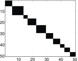
(a) Truth structure

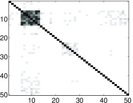
(b) GGMs

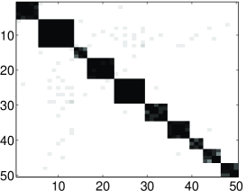
(c) Our approach

Figure 1.1: An illustrative example to justify the importance of modeling nonlinear interactions among random variables in a graphical model. The intensity of each entry is the frequency of nonzeros identified for this entry out of 10 replications. White indicates 10 zeros identified out of 10 runs, and black indicates 0/10.

1.2 Our Contribution

In this paper, we address the problem of learning pairwise UGMs with pairwise sufficient statistics defined by $\{f_{st}(X_{s},X_{t}):=\phi(X_{s},X_{t})\}$ where $\phi$ is the global parametric function. This subclass of UGMs allow us to model highly nonlinear interactions among the variables. In contrast, most existing parametric/semiparametric graphical models use pairwise product of variables (or properly transformed variables) as sufficient statistics (Ravikumar et al., 2011; Liu et al., 2009; Yang et al., 2012), and thus in their nature are unable to capture underlying complex interactions among the variables. We propose two estimators to learn the weights in the proposed UGMs. The first estimator is formulated as $\ell_{1}$-norm penalized maximum likelihood estimation (MLE). The second estimator is formulated as $\ell_{1}$-norm penalized node-wise conditional MLE. The parameters of the global mapping $\phi$ can be selected through, e.g., cross-validations.

One contribution of this paper is the statistical efficiency analysis of the proposed estimators in terms of parameter estimation error. We prove that under proper conditions the joint MLE estimator achieves convergence rate $O(\sqrt{|E|\ln p/n})$ where $|E|$ is the number of edges. For the node-wise conditional estimator, we prove that under proper conditions it achieves convergence rate $O(\sqrt{d\ln p/n})$ in which $d$ is the degree of the underlying graph $G$. For GGMs, these convergence rates are known to be minimax optimal (Yuan, 2010; Cai et al., 2011). We have also analyzed the computational efficiency of the proposed estimators. Particularly, when the mapping $\phi$ is a Mercer kernel, we show that with proper relaxation the joint MLE estimator reduces to a log-determinant program and the conditional MLE estimator reduces to a Lasso program. These relaxed estimators can be efficiently optimized using off-the-shelf algorithms.

We conduct careful numerical studies on simulated and real data to support our claims. Our simulation results show that, when the data are drawn from an underlying UGMs with highly nonlinear sufficient statistics, our approach significantly outperforms GGMs and Nonparanormal estimators in most cases. The experimental results on a stock price data show that our method recovers more accurate links than GMMs and Nonparanormal estimators. Continuing with the aforementioned illustrative example, Figure 1.1(c) shows the graph structure recovered by our proposed semi-parametric model with heat kernel $\phi(X_{s},X_{t})=\exp\{|X_{s}-X_{t}|^{2}/\sigma^{2}\}$. It can be clearly seen that our model performs well while the GGMs fail on this example.

1.3 Related Work

In order to model random variables beyond parametric UGMs such as GGMs and Ising models, researchers recently investigated semiparametric/nonparametric extensions of these parametric models. The Nonparanormal (Liu et al., 2009) and copula-based methods (Dobra & Lenkoski, 2011) are semiparametric graphical models which assume that data is Gaussian after applying a monotone transformation. The network structure of these models can be recovered by fitting GGMs over the transformed variables. This class of models are also known as Gaussian copula family (Klaassen & Wellner, 1997; Tsukahara, 2005). More broadly, one could learn transformations of the variables and then fit any parametric UGMs (e.g., EFGMs) over the transformed variables. In two recent papers (Liu et al., 2012; Xue & Zou, 2012), the rank-based estimators were used to estimate correlation matrix $\hat{S}$ and then fit the following model GGMs.

$$\mathbb{P}(X;\Omega)=\frac{1}{\sqrt{(2\pi)^{p}(\det\Omega)^{-1}}}\exp\left\{-\text{Tr}(\Omega\hat{S})\right\},$$ (1.4)

where $\Omega\succ 0$ is the precision matrix to be estimated. The sufficient statistics used in this model are encoded in the correlation matrix $\hat{S}$. Very recently, Gu et al. (2013) proposed a functional minimization framework to estimate the nonparametric model (1.1) over a Reproducing Hilbert Kernel Space (RKHS). In this framework, to infer geometric structure, a “hypothesis testing” method is used to eliminate those weak interaction terms (edges). The forest density estimation (Lafferty et al., 2012) is a fully nonparametric method for estimating UGMs with structure restricted to be a forest. Combinatorial approaches were proposed by Lauritzen (1996); Bishop et al. (2007) for fitting graphical models over multivariate count data. A kernel method was proposed by Bach & Jordan (2002) for learning the structure of graphical models by treating variables as Gaussians in a mapped high-dimensional feature space.

1.4 Notation and Outline

Notation. In the following, $\theta=(\theta_{i})\in\mathbb{R}^{p}$ is a vector; $\Theta=(\Theta_{ij})\in\mathbb{R}^{p\times p}$ is a matrix. The following notations will be used in the text.

• $\text{supp}(\theta)$: the support (set of nonzero elements) of $\theta$.

• $\|\theta\|_{0}$: the number of nonzero of $\theta$.

• $\|\theta\|_{1}=\sum_{i=1}^{p}|\theta_{i}|$: the $\ell_{1}$-norm of vector $\theta$.

• $\|\theta\|_{2}=\sqrt{\theta^{\top}\theta}$: the Euclidean norm of vector $\theta$.

• $|\Theta|_{1}=\sum_{i=1}^{p}\sum_{j=1}^{q}|\Theta_{ij}|$: the element-wise $\ell_{1}$-norm of matrix $\Theta$.

• $\|\Theta\|_{2,\infty}=\max_{j}\sqrt{\sum_{i}\Theta^{2}_{ij}}$: the max column Euclidean norm of $\Theta$.

• $\text{supp}(\Theta)=\{(i,j):\Theta_{ij}\neq 0\}$: the support of $\Theta$.

• $\text{Tr}(\Theta)$: the trace (sum of diagonal elements) of a matrix $\Theta$.

• $\Theta^{-}$: the off-diagonals of $\Theta$.

• $\Theta\succeq 0$ ($\Theta\succ 0$): $\Theta$ is a positive semi-definite (positive definite) matrix.

• $I_{m\times m}$: $m$-by-$m$ identity matrix.

• $\bar{S}$: the complement of an index set $S$.

Outline. The remaining of this paper is organized as follows: §2 introduces the semi-parametric pairwise UGMs with nonlinear sufficient statistics. §3 presents two maximum likelihood estimators for learning model parameters. The statistical guarantees of the proposed estimators are analyzed in §4. Monte-Carlo simulations and experimental results on real data are presented in §5. Finally, we conclude this paper in §6.

2 Pairwise UGMs with Nonlinear Sufficient Statistics

Given a univariate parametric mapping $f:\mathcal{X}\rightarrow\mathbb{R}$ and a bivariate parametric mapping $\phi(\cdot,\cdot):\mathcal{X}^{2}\rightarrow\mathbb{R}$ (for notation clarity purpose we do not explicitly write out the parameters in $f$ and $\phi$), we assume that the joint density of $X$ is given by the following Semiparametric Exponential Family Graphical Models (Semi-EFGMs) distribution:

$$\mathbb{P}(X;\theta)=\exp\left\{\sum_{s\in V}\theta_{s}f(X_{s})+\sum_{(s,t)\in E}\theta_{st}\phi(X_{s},X_{t})-A(\theta)\right\},$$ (2.1)

where

$$A(\theta):=\log\int_{\mathcal{X}^{p}}\exp\left\{\sum_{s\in V}\theta_{s}f(X_{s})+\sum_{(s,t)\in E}\theta_{st}\phi(X_{s},X_{t})\right\}dX$$

is the log-partition function. We require the condition $A(\theta)<\infty$ holds so that the definition of probability is valid. The node-wise sufficient statistics $\{f(X_{s})\}$ reflect the strength of individual nodes. The pairwise sufficient statistics $\{\phi(X_{s},X_{t})\}$ characterize the interactions between the nodes. Specially, when $\phi(x,y)=xy$, Semi-EFGMs reduce to the standard EFGMs with distribution (1.2). By using proper nonlinear $\phi$, Semi-EFGMs is able to capture more complex interactions among variables than EFGMs. Particularly, if the mapping function $\phi$ is chosen as a Mercer kernel and $f(X)=\phi(X,X)$, then the distribution of Semi-EFGMs is written by

$$\mathbb{P}(X;\theta)=\exp\left\{\sum_{s\in V}\theta_{s}\phi(X_{s},X_{s})+\sum_{(s,t)\in E}\theta_{st}\phi(X_{s},X_{t})-A(\theta)\right\}.$$

In this case, Semi-EFGMs can be regarded as a kernel extension of the Gaussian graphical models by replacing coefficient matrix with kernel matrix $\Phi$ whose entries are given by $\Phi_{st}=\phi(X_{s},X_{t})$. Different from GGMs, it is difficult to find a close-form log-partition function $A(\theta)$ in the above distribution. It is interesting to note that when using kernel mapping $\phi$, Semi-EFGMs allow each random variate to be vector-valued. This property is particularly useful in scenarios where each random variate is described by different modalities of features. In the current model, up to tunable parameters, the bivariate mapping $\phi$ is assumed to be known. This is analogous to kernel methods in which the kernels are conventionally assumed to be known.

3 Parameter Estimation

We are interested in the problem of learning the graph structure of an underlying Semi-EFGM given i.i.d. samples. Suppose we have $n$ independent samples $\mathbb{X}_{n}=\{X^{(i)}\}_{i=1}^{n}$ drawn from a Semi-EFGM with true parameters $\theta^{*}$:

$$\mathbb{P}(X;\theta^{*})=\exp\left\{\sum_{s\in V}f(X_{s})+\sum_{(s,t)\in E}\theta^{*}_{st}\phi(X_{s},X_{t})-A(\theta^{*})\right\}.$$ (3.1)

For the sake of notation simplicity in the analysis to follow, we have assumed here that $\theta_{s}^{*}=1$, noting that our algorithm and analysis generalize straightforwardly to the cases where $\theta_{ss}^{*}$ are also varying. An important goal of graphical model learning is to estimate the true parameters $\theta^{*}$ from the observed data $\mathbb{X}_{n}$. The more accurate parameter estimation is, the more accurate we are able to recover the underlying graph structure. In this section, we will propose two maximum likelihood estimation (MLE) methods, the $\ell_{1}$-norm penalized joint MLE and the $\ell_{1}$-norm penalized node-conditional MLE, to estimate the model parameters.

3.1 Joint Parameter Estimation

Given $n$ independent samples $\mathbb{X}_{n}=\{X^{(i)}\}_{i=1}^{n}$, we can write the log-likelihood of the joint distribution (3.1) as:

$$L(\theta;\mathbb{X}_{n})=-\frac{1}{n}\sum_{i=1}^{n}\log\mathbb{P}(X^{(i)};\theta)=-\frac{1}{n}\sum_{i=1}^{n}\left\{f(X_{s}^{(i)})+\sum_{s\neq t}\theta_{st}\phi(X^{(i)}_{s},X^{(i)}_{t})\right\}+A(\theta).$$

With a bit algebra we can obtain the following standard result which shows that the first two derivatives of $L(\theta;\mathbb{X}_{n})$ yield the cumulants of the random variables $\phi(X_{s},X_{t})$ and $L(\theta;\mathbb{X}_{n})$ is convex with respect to $\theta$ (see also, e.g., Wainwright & Jordan, 2008).

Proposition 1.

The likelihood function $L(\theta;\mathbb{X}_{n})$ has the following first two derivatives:

$$\frac{\partial L(\theta;\mathbb{X}_{n})}{\partial\theta_{st}} = -\frac{1}{n}\sum_{i=1}^{n}\phi(X^{(i)}_{s},X^{(i)}_{t})+\mathbb{E}_{\theta}[\phi(X_{s},X_{t})],$$ (3.2)

$$\frac{\partial^{2}L(\theta;\mathbb{X}_{n})}{\partial\theta_{st}\partial\theta_{uv}} = \mathbb{E}_{\theta}[\phi(X_{s},X_{t})\phi(X_{u},X_{v})]-\mathbb{E}_{\theta}[\phi(X_{s},X_{t})]\mathbb{E}_{\theta}[\phi(X_{u},X_{v})],$$ (3.3)

where the expectation $\mathbb{E}_{\theta}[\cdot]$ is taken over the joint distribution (2.1). Moreover, $L(\theta;\mathbb{X}_{n})$ is a convex function with respect to $\theta$.

In order to estimate the parameters, we consider the following $\ell_{1}$-norm penalized MLE:

$$\hat{\theta}_{n}=\mathop{\arg\min}_{\theta}\left\{L(\theta;\mathbb{X}_{n})+\lambda_{n}\|\theta\|_{1}\right\},$$ (3.4)

where $\lambda_{n}>0$ is the regularization strength parameter dependent on $n$. By Proposition 1, the M-estimator (3.4) is strongly convex, and thus admits a unique global minimizer. The solution can be found by some off-the-shelf first-order iterative algorithms such as proximal gradient descent (Nesterov, 2005; Tseng, 2008; Beck & Teboulle, 2009). At each iteration, we need to evaluate the gradient $\nabla L(\theta;\mathbb{X}_{n})$ which is given in (3.2). Note that the major computational overhead is to calculate the expectation term $\mathbb{E}_{\theta}[\phi(X_{s},X_{t})]$. In general, this term has no close-form for exact calculation. We have to resort to sampling methods for approximate estimation. The multivariate sampling methods, however, typically suffer from high computational cost especially when dimension $p$ is large. We next consider the node-wise parameter estimation method which only requires univariate sampling for computing the expectation terms involved in the gradient.

3.2 Node-wise Parameter Estimation

Recent state of the art methods for learning GGMs, Ising models and exponential family models (Meinshausen & Bühlmann, 2006; Ravikumar et al., 2010; Yang et al., 2012) suggest a natural procedure for deriving multivariate graphical models from univariate distributions. The key idea in those methods is to learn the MRF graph structure by estimating node-neighborhoods, or by fitting node-conditional distributions of each node conditioned on the rest of the nodes. Indeed, these node-wise fitting methods have been shown to have strong computational as well as statistical guarantees. Following these approaches, we propose an alternative estimator which estimates the weights of sufficient statistics associated with each individual node. Given the joint distribution (3.1), it is easy to show that the conditional distribution of $X_{s}$ given the rest variables, $X_{\setminus s}$, is written by:

$$\mathbb{P}(X_{s}\mid X_{\setminus s};\theta^{*}_{s})=\exp\left\{f(X_{s})+\sum_{t\in N(s)}\theta^{*}_{st}\phi(X_{s},X_{t})-D(X_{\setminus s};\theta^{*}_{s})\right\},$$ (3.5)

where with slight abuse of notations, we denote $\theta^{*}_{s}:=\{\theta^{*}_{st}\}_{t\in N(s)}$, and

$$D(X_{\setminus s};\theta^{*}_{s}):=\log\int_{\mathcal{X}}\exp\left\{f(X_{s})+\sum_{t\in N(s)}\theta^{*}_{st}\phi(X_{s},X_{t})\right\}dX_{s}$$

is the log-partition function which ensures normalization. Indeed, the marginal distribution of $X_{\setminus s}$ is

$$\mathbb{P}(X_{\setminus s};\theta^{*})=\int_{\mathcal{X}}\mathbb{P}(X;\theta^{*})dX_{s}=\exp\left\{\sum_{u\in V\setminus s}f(X_{u})+\sum_{(u,t)\in E,u\in V\setminus s}\theta^{*}_{ut}\phi(X_{u},X_{t})-A(\theta^{*})+D(X_{\setminus s};\theta^{*}_{s})\right\}.$$

The conditional distribution (3.5) is then $\mathbb{P}(X_{s}\mid X_{\setminus s};\theta^{*})=\mathbb{P}(X;\theta^{*})/\mathbb{P}(X_{\setminus s};\theta^{*})$. We note that $A(\theta^{*})<\infty$ implies $D(X_{\setminus s};\theta^{*}_{s})<\infty$.

In order to estimate the parameters associated with any node, we consider using the sparsity constrained conditional maximum likelihood estimation. Given $n$ independent samples $\mathbb{X}_{n}$, we can write the log-likelihood of the conditional distribution (3.5) as:

$$\tilde{L}(\theta_{s};\mathbb{X}_{n})=-\frac{1}{n}\sum_{i=1}^{n}\log\mathbb{P}(X^{(i)}_{s}\mid X^{(i)}_{\setminus s};\theta_{s})=\frac{1}{n}\sum_{i=1}^{n}\left\{-f(X^{(i)}_{s})-\sum_{t\neq s}\theta_{st}\phi(X^{(i)}_{s},X^{(i)}_{t})+D(X^{(i)}_{\setminus s};\theta_{s})\right\},$$

where $\theta_{s}=(\theta_{st})_{t\neq s}\in\mathbb{R}^{p-1}$ is the set of parameter to be estimated. Analogous to Proposition 1, the following proposition gives the first two derivatives of the likelihood function $\tilde{L}(\theta_{s};\mathbb{X}_{n})$ and establishes the convexity of $\tilde{L}(\theta_{s};\mathbb{X}_{n})$.

Proposition 2.

The likelihood function $\tilde{L}(\theta_{s};\mathbb{X}_{n})$ has the following first two derivatives:

$$\frac{\partial\tilde{L}(\theta_{s};\mathbb{X}_{n})}{\partial\theta_{st}} = \frac{1}{n}\sum_{i=1}^{n}\left\{-\phi(X_{s}^{(i)},X_{t}^{(i)})+\mathbb{E}_{\theta_{s}}[\phi(X_{s},X_{t}^{(i)})\mid X^{(i)}_{\setminus s}]\right\},$$ (3.6)

$$\frac{\partial^{2}\tilde{L}(\theta_{s};\mathbb{X}_{n})}{\partial\theta_{st}\partial\theta_{su}} = \frac{1}{n}\sum_{i=1}^{n}\left\{\mathbb{E}_{\theta_{s}}[\phi(X_{s},X_{t}^{(i)})\phi(X_{s},X_{u}^{(i)})\mid X^{(i)}_{\setminus s}]\right.$$ (3.7)

$$\left.-\mathbb{E}_{\theta_{s}}[\phi(X_{s},X_{t}^{(i)})\mid X^{(i)}_{\setminus s}]\mathbb{E}_{\theta_{s}}[\phi(X_{s},X_{u}^{(i)})\mid X^{(i)}_{\setminus s}]\right\},$$

where the expectation $\mathbb{E}_{\theta_{s}}[\cdot\mid X_{\setminus s}]$ is taken over the node-wise conditional distribution (3.5). Moreover, $\tilde{L}(\theta_{s};\mathbb{X}_{n})$ is a convex function with respect to $\theta_{s}$.

Let us consider the following $\ell_{1}$-norm penalized conditional MLE formulation associated with the variable $X_{s}$:

$$\hat{\theta}^{n}_{s}=\mathop{\arg\min}_{\theta_{s}}\left\{\tilde{L}(\theta_{s};\mathbb{X}_{n})+\lambda_{n}\|\theta_{s}\|_{1}\right\},$$ (3.8)

where $\lambda_{n}>0$ is the regularization strength parameter dependent on $n$. By Proposition 2, the above M-estimator is strongly convex, and thus admits a unique global minimizer. We can use standard first-order methods such as proximal gradient descent algorithms to optimize the estimator (3.8). At each iteration, we need to evaluate the gradient $\nabla\tilde{L}(\theta_{s};\mathbb{X}_{n})$ which is given by (3.6). Note that the major computational overhead of (3.6) is to calculate the expectation term $\mathbb{E}_{\theta_{s}}[\phi(X_{s},X_{t}^{(i)})\mid X^{(i)}_{\setminus s}]$. When $X_{s}$ is finite and discrete, this term can be computed exactly via summation. For count-valued or real-valued variables, however, this term is typically lack of a close-form for exact calculation. We may resort to some standard univariate sampling methods, e.g., importance sampling and MCMC (Bishop, 2006), to approximately estimate this expectation term. The univariate sampling process required by the node-wise estimator (3.8) is much more computational efficient than the multivariate sampling process required by the joint estimator (3.4).

4 Statistical Analysis

We now provide some parameter estimation error bounds for the joint MLE estimator (3.4) and the node-conditional estimator (3.8). In large picture, we use the techniques from (Negahban et al., 2012; Zhang & Zhang, 2012) to analyze our model by specifying the conditions under which these techniques can be applied to the model.

4.1 Analysis of the Joint Estimator

For the joint estimator (3.4), we study the convergence rate of the parameter estimation error $\|\hat{\theta}_{n}-\theta^{*}\|$ as a function of sample size $n$. Intuitively, as $n\rightarrow\infty$, we expect $\hat{\theta}_{n}\rightarrow\theta^{*}$ and thus $\nabla L(\hat{\theta}_{n};\mathbb{X}_{n})\rightarrow\nabla L(\theta^{*};\mathbb{X}_{n})$. Since $\hat{\theta}_{n}$ is the minimizer of (3.4), we have $\nabla L(\hat{\theta}_{n};\mathbb{X}_{n})\rightarrow 0$ as $n\rightarrow\infty$ and $\lambda_{n}\rightarrow 0$. Therefore it is desired that $\nabla L(\theta^{*};\mathbb{X}_{n})$ approaches zero as $n$ approaches infinity. Inspired by this intuition and Proposition 1, we are interested in the concentration bound of the random variables defined by

$$Z_{st}:=\phi(X_{s},X_{t})-\mathbb{E}_{\theta^{*}}[\phi(X_{s},X_{t})],$$

where the expectation $\mathbb{E}_{\theta^{*}}[\cdot]$ is taken over the underlying true distribution (3.1). By the “law of the unconscious statistician” we know that $\mathbb{E}[Z_{st}]=\mathbb{E}_{\theta^{*}}[\phi(X_{s},X_{t})]-\mathbb{E}_{\theta^{*}}[\phi(X_{s},X_{t})]=0$. That is, $Z_{st}$ are zero-mean random variables. We introduce the following technical condition on $Z_{st}$ which we will show that guarantees the gradient $\nabla L(\theta^{*};\mathbb{X}_{n})$ vanishes exponentially fast, with high probability, as sample size increases.

Assumption 1.

For all $(s,t)$, we assume that there exist constants $\sigma>0$ and $\zeta>0$ such that for all $|\eta|\leq\zeta$,

$$\mathbb{E}[\exp\{\eta Z_{st}\}]\leq\exp\left\{\sigma^{2}\eta^{2}/2\right\}.$$

This assumption essentially imposes an exponential-type bound on the moment generating function of the random variables $Z_{st}$. Equivalently, from the definition of $Z_{st}$ and the “law of the unconscious statistician” we know that this assumptions requires:

$$\mathbb{E}_{\theta^{*}}[\exp\{\eta(\phi(X_{s},X_{t})-\mathbb{E}_{\theta^{*}}[\phi(X_{s},X_{t})])\}]\leq\exp\left\{\sigma^{2}\eta^{2}/2\right\}.$$

The following result indicates that under Assumption 1, $Z_{st}$ satisfy a large deviation inequality.

Lemma 1.

If Assumption 1 holds, then for all index pairs $(s,t)$ and any $\varepsilon\leq\sigma^{2}\zeta$ we have

$$\mathbb{P}\left(\left|\frac{1}{n}\sum_{i=1}^{n}\phi(X^{(i)}_{s},X^{(i)}_{t})-\mathbb{E}_{\theta^{*}}[\phi(X_{s},X_{t})]\right|>\varepsilon\right)\leq 2\exp\left\{-\frac{n\varepsilon^{2}}{2\sigma^{2}}\right\}.$$

A proof of this lemma is given in Appendix A.1. As we will see in the analysis to follow that Lemma 1 plays a key role in the deviation of the convergence rate of the joint MLE estimator (3.4). Before proceeding, we give a few remarks on the conditions under which the random variables $Z_{st}$ satisfy Assumption 1 such that Lemma 1 holds.

Remark 1 ($Z_{st}$ are sub-Gaussian).

We call a zero-mean random variable $Z$ sub-Gaussian if there exists a constant $\sigma>0$ such that $\mathbb{E}[\exp\{\eta Z\}]\leq\exp\left\{\sigma^{2}\eta^{2}/2\right\},\text{for all }\eta\in\mathbb{R}$. It is straightforward to see that Assumption 1 holds when $Z_{st}$ are sub-Gaussian random variables. For zero-mean Gaussian random variable $Z\sim N(0,\sigma^{2})$, it can be verified that $\mathbb{E}[\exp\{\eta Z\}]=\exp\{\sigma^{2}\eta^{2}/2\}$. Based on the Hoeffding’s Lemma, for any random variable $Z\in[a,b]$ and $\mathbb{E}[z]=0$, we have $\mathbb{E}[\exp\{\eta Z\}]\leq\exp\{\eta^{2}(b-a)^{2}/8\}$. Therefore, Assumption 1 holds when $Z_{st}$ are zero-mean Gaussian or zero-mean bounded random variables. For an instance, Assumption 1 is valid when the heat kernel mapping $\phi(X_{s},X_{t})=\exp\{-|X_{s}-X_{t}|^{2}\}$ is used.

Remark 2 ($Z_{st}$ are sub-exponential).

We call a random variable $Z$ sub-exponential if there exist constants $c_{1},c_{2}>0$ such that $\mathbb{P}(|X|>\eta)\leq\exp\left\{c_{1}-\eta/c_{2}\right\},\text{for all }t\in\mathbb{R}$. Using the result in (Vershynin, 2011, Lemma 5.15), we can verify that Assumption 1 holds when $Z_{st}$ are sub-exponential random variables. One connection between sub-Gaussian and sub-exponential random variables is: a random variable $Z$ is sub-Gaussian if and only if $Z^{2}$ is sub-exponential (Vershynin, 2011, Lemma 5.14). From this connection and the fact that the sum of sub-exponential random variables is still exponential, we know that if $Z_{st}$ are Chi-square random variables (sum of square of Gaussian), then $Z_{st}$ are sub-exponential and thus Assumption 1 holds.

Remark 3.

More generally, consider that $\phi$ is a Mercer kernel satisfying the condition:

$$\int_{\mathcal{X}}\exp\{-c\phi(X,X)\}dX<\infty,\quad\text{for any }c>0.$$ (4.1)

Obviously, this condition holds when $\phi(X,X)$ grows faster than $X^{q}$ for some $q>0$. If $f(X_{s})=-\phi(X_{s},X_{s})$ and $|\theta^{*}_{st}|<0.25$, then we claim that $Z_{st}$ are sub-exponential. Indeed, since $\phi$ is Mercer kernel, we have that $\phi(X_{s},X_{s})\geq 0$, $\phi(X_{s},X_{t})=\phi(X_{t},X_{s})$ and $|\phi(X_{s},X_{t})|\leq(\phi(X_{s},X_{s})+\phi(X_{t},X_{t}))/2$. Thus,

$$\mathbb{P}(|\phi(X_{s},X_{t})|>\eta)\leq\mathbb{P}(\phi(X_{s},X_{s})+\phi(X_{t},X_{t})>2\eta).$$ (4.2)

For any $s\in V$, from the joint distribution (3.1) and $|\theta^{*}_{st}|<0.25$ we know that the marginal distribution of $X_{s}$ is bounded by $\mathbb{P}(X_{s})\leq c_{1}\exp\left\{-\phi(X_{s},X_{s})/2\right\}$ for some absolute constant $c_{1}$. Therefore, by using Markov inequality and (4.1) we obtain that for any $\eta>0$

$$\mathbb{P}(\phi(X_{s},X_{s})>\eta)\leq\frac{\mathbb{E}[\exp\{\phi(X_{s},X_{s})/4\}]}{\exp\{\eta/4\}}\leq\frac{c_{1}\int_{\mathcal{X}}\exp\{-\phi(X_{s},X_{s})/4\}dX_{s}}{\exp\{\eta/4\}}\propto\exp\{-\eta/4\},$$

which implies that $\phi(X_{s},X_{s})$ is sub-exponential. By combining the fact that the sum of sub-exponential random variables is still sub-exponential and (4.2) we obtain that $\phi(X_{s},X_{t})$ are sub-exponential, and so are $Z_{st}$. Obviously, the above claim is applicable to the case of multivariate Gaussian where $\phi(X_{s},X_{t})=X_{s}X_{t}$ and $f(X_{s})=-X_{s}^{2}$. Similar results have also been proved in previous work on GGMs (Rothman et al., 2008; Ravikumar et al., 2011).

Let us define $\gamma_{n}:=\|\nabla L(\theta^{*};\mathbb{X}_{n})\|_{\infty}$. The following lemma indicates that under Assumption 1, with overwhelming probability, $\gamma_{n}$ approaches zero at the rate of $O(\sqrt{\ln p/n})$. A proof of this lemma can be found in Appendix A.2.

Lemma 2.

Assume that Assumption 1 holds. If $n>6\ln p/(\sigma^{2}\zeta^{2})$, then with probability at least $1-2p^{-1}$ the following inequality holds:

$$\gamma_{n}=\|\nabla L(\theta^{*};\mathbb{X}_{n})\|_{\infty}\leq\sigma\sqrt{6\ln p/n}.$$

From (3.3) we know that the Hessian $\nabla^{2}L(\theta;\mathbb{X}_{n})$ is positive semidefinite at any $\theta$. To derive the estimation error, we also need the following condition which guarantees the restricted positive definiteness of $\nabla^{2}L(\theta;\mathbb{X}_{n})$ when $\theta$ is sufficiently close to $\theta^{*}$.

Assumption 2 (Locally Restricted Positive Definite Hessian).

Let $S=\text{supp}(\theta^{*})$. There exist constants $r>0$ and $\beta>0$ such that for any $\theta\in\{\|\theta-\theta^{*}\|<r\}$, the following inequality holds for any $\vartheta\in\mathcal{C}_{S}:=\{\|\theta_{\bar{S}}\|_{1}\leq 3\|\theta_{S}\|_{1}\}$:

$$\vartheta^{\top}\nabla^{2}L(\theta;\mathbb{X}_{n})\vartheta\geq\beta\|\vartheta\|^{2}.$$

Assumption 2 requires that the Hessian $\nabla^{2}L(\theta;\mathbb{X}_{n})$ is positive definite in the cone $\mathcal{C}_{S}$ when $\theta$ lies in a local ball centered at $\theta^{*}$. This condition is specification of the concept restricted strong convexity (Zhang & Zhang, 2012) to our problem setup. If $X$ is multivariate Gaussian, i.e., $\phi(X_{s},X_{t})=X_{s}X_{t}$ and $f(X_{s})=-X_{s}^{2}$, it is easy to verify that this condition can be satisfied when the true precision matrix is positive definite (Rothman et al., 2008).

Remark 4 (Minimal Representation).

We say Semi-EFGM has minimal representation if there is a unique parameter vector $\theta$ associate with the distribution (2.1). When fix $\theta_{ss}=1$, this condition equivalently requires that there does not exist a non-zero $\theta$ such that the linear combination $\sum_{s,t}\theta_{st}\phi(X_{s},X_{t})$ is equal to an absolute constant. This implies that for any $\theta$,

$$\text{Var}_{\theta}\left[\sum_{s,t}\vartheta_{st}\phi(X_{s},X_{t})\right]=\vartheta^{\top}\nabla^{2}L(\theta;\mathbb{X}_{n})\vartheta>0,\quad\text{for all non-zero $\vartheta$}.$$

It follows that there exist constants $r>0$ and $\beta>0$ such that for any $\theta\in\{\|\theta-\theta^{*}\|<r\}$, $\vartheta^{\top}\nabla^{2}L(\theta;\mathbb{X}_{n})\vartheta\geq\beta\|\vartheta\|^{2}$. Therefore, Assumption 2 is valid when Semi-EFGM has minimal representation.

The following result bounds the estimation error of the joint MLE estimator (3.4) in terms of $\gamma_{n}$, $r$ and $\beta$.

Lemma 3.

Assume that the conditions in Assumption 2 hold. Assume that $\lambda_{n}\in[2\gamma_{n},c_{0}\gamma_{n}]$ for some $c_{0}\geq 2$. Define $\gamma=1.5c_{0}\sqrt{\|\theta^{*}\|_{0}}\beta^{-1}\gamma_{n}$. If $\gamma<r$, then we have

$$\|\hat{\theta}_{n}-\theta^{*}\|\leq 1.5\sqrt{\|\theta^{*}\|_{0}}\beta^{-1}\gamma_{n}.$$

A proof of this lemma is provided in Appendix A.3. The following theorem is our main result on the estimation error of the joint MLE estimator (3.4).

Theorem 1.

Assume that the conditions in Lemma 2 and Lemma 3 hold. If sample size $n$ satisfies

$$n>\max\left(\frac{6\ln p}{\sigma^{2}\zeta^{2}},13.5c_{0}^{2}r^{-2}\beta^{-2}\sigma^{2}\|\theta^{*}\|_{0}\ln p\right),$$

then with probability at least $1-2p^{-1}$, the following inequality holds:

$$\|\hat{\theta}_{n}-\theta^{*}\|\leq 1.5c_{0}\beta^{-1}\sigma\sqrt{6\|\theta^{*}\|_{0}\ln p/n}.$$

Proof.

By using Lemma 2 and the condition $n>13.5c_{0}^{2}r^{-2}\beta^{-2}\sigma^{2}\|\theta^{*}\|_{0}\ln p$ we have that with probability at least $1-2p^{-1}$,

$$\gamma=1.5c_{0}\sqrt{\|\theta^{*}\|_{0}}\beta^{-1}\gamma_{n}\leq 1.5c_{0}\beta^{-1}\sigma\sqrt{6\|\theta^{*}\|_{0}\ln p/n}<r.$$

By applying Lemma 3 we obtain the desired result. ∎

Remark 5.

The main message Theorem 1 conveys is that when $n=O(\|\theta^{*}\|_{0}\ln p)$ is sufficiently large, the estimation error $\|\hat{\theta}_{n}-\theta^{*}\|$ vanishes at the order of $O(\sqrt{\|\theta^{*}\|_{0}\ln p/n})$. This convergence rate matches the results obtained in (Rothman et al., 2008; Ravikumar et al., 2011) for GGMs and the results in (Liu et al., 2012; Xue & Zou, 2012) for Nonparanormal. To our knowledge, this is the first sparse recovery result for the exponential family graphical models with general sufficient statistics beyond pairwise product. Note that we did not make any attempt to optimize the constants in Theorem 1, which are relatively loose.

By specifying the conditions under which the assumptions in Theorem 1 hold, we obtain the following corollary.

Corollary 1.

Assume that the mapping function $\phi(\cdot,\cdot)$ is a Mercer kernel satisfying the condition (4.1). Let $f(X_{s})=-\phi(X_{s},X_{s})$. Assume that the joint distribution (3.1) has minimal representation and $|\theta^{*}_{st}|\leq 0.25$. Then there exist constants $\sigma,\zeta,r,\beta,c_{0}>0$ such that if

$$n>\max\left(\frac{6\ln p}{\sigma^{2}\zeta^{2}},13.5c_{0}^{2}r^{-2}\beta^{-2}\sigma^{2}\|\theta^{*}\|_{0}\ln p\right),$$

then with probability at least $1-2p^{-1}$, the following inequality holds:

$$\|\hat{\theta}_{n}-\theta^{*}\|\leq 1.5c_{0}\beta^{-1}\sigma\sqrt{6\|\theta^{*}\|_{0}\ln p/n}.$$

Proof.

Since $\phi(\cdot,\cdot)$ is a Mercer kernel satisfying (4.1) and $f(X_{s})=-\phi(X_{s},X_{s})$, from the arguments in Remark 3 we know that $Z_{st}:=\phi(X_{s},X_{t})-\mathbb{E}_{\theta^{*}}[\phi(X_{s},X_{t})]$ are sub-exponential, and thus Assumption 1 holds. Since the joint distribution (3.1) has minimal representation, from the discussions in Remark 4 we know that Assumption 2 is valid. The corollary then follows immediately from Theorem 1. ∎

4.2 Analysis of the Node-Conditional Estimator

For the node-conditional estimator (3.8), we study the rate of convergence of the parameter estimation error $\|\hat{\theta}^{n}_{s}-\theta^{*}_{s}\|$ as a function of sample size $n$. Intuitively, as $n\rightarrow\infty$, we expect $\hat{\theta}^{n}_{s}\rightarrow\theta^{*}_{s}$ and thus $\nabla\tilde{L}(\hat{\theta}^{n}_{s};\mathbb{X}_{n})\rightarrow\nabla\tilde{L}(\theta^{*}_{s};\mathbb{X}_{n})$. Since $\hat{\theta}^{n}_{s}$ is the minimizer of (3.8), we have $\nabla\tilde{L}(\hat{\theta}^{n}_{s};\mathbb{X}_{n})\rightarrow 0$ as $n\rightarrow\infty$ and $\lambda_{n}\rightarrow 0$. Therefore it is desired that $\nabla\tilde{L}(\theta^{*}_{s};\mathbb{X}_{n})$ vanishes as $n$ approaches infinity. Inspired by this intuition and Proposition 2, we study the concentration bound of the random variables defined by

$$\tilde{Z}_{st}:=\mathbb{E}_{\theta^{*}_{s}}[\phi(X_{s},X_{t})\mid X_{\setminus s}]-\mathbb{E}_{\theta^{*}}[\phi(X_{s},X_{t})],$$

where the expectation $\mathbb{E}_{\theta^{*}_{s}}[\cdot\mid X_{\setminus s}]$ is taken over the node-conditional distribution (3.5). By applying the “law of the unconscious statistician” and the rule of iterated expectation (i.e., $\mathbb{E}[X]=\mathbb{E}[\mathbb{E}[X|Y]]$), we obtain that $\mathbb{E}[\tilde{Z}_{st}]=\mathbb{E}_{\theta^{*}}[\phi(X_{s},X_{t})]-\mathbb{E}_{\theta^{*}}[\phi(X_{s},X_{t})]=0$. That is, $\tilde{Z}_{st}$ are zero-mean random variables. The following lemma shows that under Assumption 1, $\tilde{Z}_{st}$ have exponential-type moment generating function. A proof of this lemma is given in Appendix A.4.

Lemma 4.

If Assumption 1 holds, then for any $(s,t)$ we have that for all $|\eta|\leq\zeta$,

$$\mathbb{E}[\exp\{\eta\tilde{Z}_{st}\}]\leq\exp\left\{\sigma^{2}\eta^{2}/2\right\}.$$

Remark 6.

This lemma shows that the random variables $\tilde{Z}_{st}$ all have the same exponential-type moment generating function as that of $Z_{st}$. From the discussions in Remarks 1, 2 and 3 we know that when $Z_{st}$ are sub-Gaussian or sub-exponential, if Assumption 1 holds, and consequently Lemma 4 holds.

The following result indicates that under Assumption 1, $\tilde{Z}_{st}$ has a similar large deviation property as $Z_{st}$.

Lemma 5.

If Assumption 1 holds, then for all index pairs $(s,t)$ and any $\varepsilon\leq\sigma^{2}\zeta$ we have

$$\mathbb{P}\left(\left|\frac{1}{n}\sum_{i=1}^{n}\mathbb{E}_{\theta^{*}_{s}}[\phi(X_{s},X^{(i)}_{t})\mid X^{(i)}_{\setminus s}]-\mathbb{E}_{\theta^{*}}[\phi(X_{s},X_{t})]\right|>\varepsilon\right)\leq 2\exp\left\{-\frac{n\varepsilon^{2}}{2\sigma^{2}}\right\}.$$

The proof of this lemma follows the same arguments as that of Lemma 1. Let us define $\tilde{\gamma}_{n}:=\|\nabla\tilde{L}(\theta^{*}_{s};\mathbb{X}_{n})\|_{\infty}$. The following lemma indicates that under Assumption 1, with overwhelming probability, $\tilde{\gamma}_{n}$ approaches zero at the rate of $O(\sqrt{\ln p/n})$.

Lemma 6.

Assume that Assumption 1 holds. If $n>6\ln p/(\sigma^{2}\zeta^{2})$, then with probability at least $1-4p^{-2}$ the following inequality holds:

$$\tilde{\gamma}_{n}\leq 2\sigma\sqrt{6\ln p/n}.$$

A proof of this lemma can be found in Appendix A.5. Analogous to Assumption 2 for the joint estimator, we further introduce the following condition which is sufficient to guarantee the statistical efficiency of the node-conditional estimator (3.8).

Assumption 3.

For any node $s$, let $S=\text{supp}(\theta_{s}^{*})$. There exist constants $\tilde{r}>0$ and $\tilde{\beta}>0$ such that for any $\theta_{s}\in\{\|\theta_{s}-\theta_{s}^{*}\|<\tilde{r}\}$, the following inequality holds for any $\vartheta_{s}\in\tilde{\mathcal{C}}_{S}:=\{\|(\theta_{s})_{\bar{S}}\|_{1}\leq 3\|(\theta_{s})_{S}\|_{1}\}$:

$$\vartheta_{s}^{\top}\nabla^{2}\tilde{L}(\theta_{s};\mathbb{X}_{n})\vartheta_{s}\geq\tilde{\beta}\|\vartheta_{s}\|^{2}.$$

Remark 7.

Assumption 3 requires that the Hessian $\nabla^{2}\tilde{L}(\theta_{s};\mathbb{X}_{n})$ is positive definite in the cone $\tilde{\mathcal{C}}_{S}$ when $\theta_{s}$ lies in a local ball centered at $\theta_{s}^{*}$. Specially, when $X$ is multivariate Gaussian, i.e., $\phi(X_{s},X_{t})=X_{s}X_{t}$ and $f(X_{s})=-X_{s}^{2}$, this condition essentially requires that the design matrix $A^{n}_{s}=\frac{1}{n}\sum_{i=1}^{n}X^{(i)}_{\setminus s}(X^{(i)}_{\setminus s})^{\top}$ is positive definite. In this case, if the precision matrix is positive definite, then it is known from the compressed sensing literature (see Baraniuk et al., 2008; Candès et al., 2011, for example) that with overwhelming probability, $A^{n}_{s}$ is positive definite provided that the sample size $n=O(\ln p)$ is sufficiently large. More generally, it can be verified that $\mathbb{E}[\nabla^{2}\tilde{L}(\theta_{s};\mathbb{X}_{n})]$ is the sub-matrix of $\nabla^{2}L(\theta;\mathbb{X}_{n})$ associated with the pairs $(s,t)_{t\in V\setminus s}$. Therefore, if the whole Hessian matrix $\nabla^{2}L(\theta;\mathbb{X}_{n})$ is positive definite at any $\theta$, then $\mathbb{E}[\nabla^{2}\tilde{L}(\theta_{s};\mathbb{X}_{n})]$ is also positive definite. By using weak law of large number we obtain that Assumption 3 holds with high probability when $n$ is sufficiently large.

The following result establishes the estimation error of the node-conditional estimator (3.8) in terms of $\tilde{\gamma}_{n}$, $\tilde{r}$ and $\tilde{\beta}$.

Lemma 7.

Assume that the conditions in Assumption 3 hold. Assume that $\lambda_{n}\in[2\tilde{\gamma}_{n},\tilde{c}_{0}\tilde{\gamma}_{n}]$ for some $\tilde{c}_{0}\geq 2$. Define $\tilde{\gamma}=1.5\tilde{c}_{0}\sqrt{\|\theta_{s}^{*}\|_{0}}\tilde{\beta}^{-1}\tilde{\gamma}_{n}$. If $\tilde{\gamma}<\tilde{r}$, then we have

$$\|\hat{\theta}^{n}_{s}-\theta_{s}^{*}\|\leq 1.5\tilde{c}_{0}\sqrt{\|\theta_{s}^{*}\|_{0}}\tilde{\beta}^{-1}\tilde{\gamma}_{n}.$$

The proof of this lemma mirrors that of Lemma 3. By combining Lemma 6 and Lemma 7, we immediately obtain the following main result on the convergence rate of $\|\hat{\theta}^{n}_{s}-\theta^{*}_{s}\|$.

Theorem 2.

Assume that the conditions in Lemma 6 and Lemma 7 hold. If sample size $n$ satisfies

$$n>\max\left(\frac{6\ln p}{\sigma^{2}\zeta^{2}},54\tilde{c}_{0}^{2}\tilde{r}^{-2}\tilde{\beta}^{-2}\sigma^{2}\|\theta_{s}^{*}\|_{0}\ln p\right),$$

then with probability at least $1-4p^{-2}$, the following inequality holds:

$$\|\hat{\theta}^{n}_{s}-\theta^{*}_{s}\|\leq 3\tilde{c}_{0}\tilde{\beta}^{-1}\sigma\sqrt{6\|\theta^{*}_{s}\|_{0}\ln p/n}.$$

Proof.

By using Lemma 6 and the condition $n>54\tilde{c}^{2}_{0}\tilde{r}^{-2}\tilde{\beta}^{-2}\sigma^{2}\|\theta_{s}^{*}\|_{0}\ln p$ we have that with probability at least $1-4p^{-2}$,

$$\tilde{\gamma}=1.5\tilde{c}_{0}\sqrt{\|\theta^{*}_{s}\|_{0}}\tilde{\beta}^{-1}\tilde{\gamma}_{n}\leq 3\tilde{c}_{0}\tilde{\beta}^{-1}\sigma\sqrt{6\|\theta_{s}^{*}\|_{0}\ln p/n}<\tilde{r}.$$

By applying Lemma 7 we obtain the desired result. ∎

Remark 8.

Note that we did not make any attempt to optimize the constants in the presented results above, which are relatively loose. Therefore in the discussion, we shall ignore the constants, and focus on the main messages these results convey. Theorem 2 indicates that with overwhelming probability, the estimation error $\|\hat{\theta}^{n}_{s}-\theta^{*}_{s}\|=O(\sqrt{d\ln p/n})$ where $d$ is the degree of the underlying graph, i.e., $d=\max_{s\in V}\|\theta^{*}_{s}\|_{0}$. We may combine the estimation errors from all the nodes as a global measurement of accuracy. Let $\theta^{*}$ (or $\hat{\theta}^{n}$) be a matrix stacked by the columns $\theta^{*}_{s}$ (or $\hat{\theta}^{n}_{s}$). By Theorem 2 and union of probability we obtain that $\|\hat{\theta}-\theta^{*}\|_{2,\infty}=O(\sqrt{d\ln p/n})$ holds with probability at least $1-4p^{-1}$. This estimation error bound is analogous to those specifically derived for GGMs with neighborhood-selection-type estimators (Yuan, 2010).

By specifying the conditions under which the assumptions in Theorem 2 hold, we obtain the following corollary.

Corollary 2.

Assume that the mapping function $\phi(\cdot,\cdot)$ is a Mercer kernel satisfying (4.1). Let $f(X_{s})=-\phi(X_{s},X_{s})$. Assume that the joint distribution (3.1) has minimal representation and $|\theta^{*}_{st}|<0.25$. If $n$ is sufficiently large, then with overwhelming probability the following inequality holds:

$$\|\hat{\theta}^{n}_{s}-\theta^{*}_{s}\|=O(\sqrt{\|\theta_{s}^{*}\|_{0}\ln p/n}).$$

Proof.

Since $\phi(\cdot,\cdot)$ is a Mercer kernel satisfying (4.1) and $f(X_{s})=-\phi(X_{s},X_{s})$, from Remark 3 we know that $Z_{st}:=\phi(X_{s},X_{t})-\mathbb{E}_{\theta^{*}}[\phi(X_{s},X_{t})]$ are sub-exponential, and thus Assumption 1 holds. Since the joint distribution (3.1) has minimal representation, from the discussions in Remark 4 we know that Hessian $\nabla^{2}L(\theta;\mathbb{X}_{n})$ is positive definite at any $\theta$. Therefore, based on the discussions in Remark 7 we obtain that if $n$ is sufficiently large, then with overwhelming probability Assumption 3 holds. The corollary then follows immediately from Theorem 2. ∎

5 Experiment

We evaluate the performance of Semi-EFGMs for graphical models learning on synthetic and real data sets. We first investigate support recovery accuracy using simulation data (for which we know the ground truth), and then we apply our method to the analysis of a stock price data. But, before presenting the experimental results, we first need to discuss some implementation issues of the proposed estimators.

5.1 Implementation Issues

As discussed in §3.1 and §3.2, in order to estimate the gradient of the likelihood functions $L(\theta;\mathbb{X}_{n})$ and $\tilde{L}(\theta_{s};\mathbb{X}_{n})$, we need to iteratively use sampling methods to calculate the involved expectation terms. This can be quite time consuming when the dimension $p$ is large. In our empirical study, we are particularly interested in Semi-EFGMs with Mercer kernel mapping $\phi$. For this subclass of Semi-EFGMs, instead of using the generic sampling based optimization algorithms, we propose to relax the estimators (3.4) and (3.8) such that the sampling step can be avoided during the optimization.

Given a Mercer kernel $\phi$, it is possible to find a space $\mathcal{F}$ and a map $\varphi$ from $\mathcal{X}$ to $\mathcal{F}$, such that $\phi(X_{s},X_{t})=\varphi(X_{s})^{\top}\varphi(X_{t})$ is the dot produce in $\mathcal{F}$ between $\varphi(X_{s})$ and $\varphi(X_{t})$. The space $\mathcal{F}$ is usually referred to as the feature space and the map $\varphi$ as the feature map.

Relax the Joint Estimator (3.4). Assume that the feature space $\mathcal{F}$ has finite dimension $m$. Let $\varphi(X)=[\varphi(X_{1}),...,\varphi(X_{p})]\in\mathcal{F}^{p}\subseteq\mathbb{R}^{pm}$ be the expanded random vector. Provided that $X$ has the distribution (2.1) with $f(X_{s})=-\phi(X_{s},X_{s})$, the joint distribution of the random vector $\varphi(X)$ is written by

$$\mathbb{P}(\varphi(X);\Omega)\propto\exp\left\{-\varphi(X)^{\top}\Omega\varphi(X)\right\},\quad\varphi(X)\in\mathcal{F}^{p},$$ (5.1)

where $\Omega=\Theta\otimes I_{m\times m}$ and $\Theta$ is coefficient matrix with $\Theta_{ss}=1$ and $\Theta_{st}=-\theta_{st}$, $s\neq t$. Typically, the distribution (5.1) has no close-form log-partition function. Ideally, if $\mathcal{F}^{p}=\mathbb{R}^{pm}$ and $\Theta\succ 0$ (which implies $\Omega\succ 0$), then $\varphi(X)$ is multivariate Gaussian with distribution

$$\mathbb{P}(\varphi(X);\Omega)=\frac{1}{\sqrt{\pi^{pm}(\det\Omega)^{-1}}}\exp\left\{-\varphi(X)^{\top}\Omega\varphi(X)\right\}.$$

Since $\phi(X_{s},X_{t})=\varphi(X_{s})^{\top}\varphi(X_{t})$ and using the fact $\det\Omega=(\det\Theta)^{m}$, we can re-write the preceding distribution in terms of $\Theta$ as

$$\mathbb{P}(\varphi(X);\Theta)=\frac{1}{\sqrt{\pi^{pm}(\det\Theta)^{-m}}}\exp\left\{-\text{Tr}(\Theta^{\top}\Phi(X))\right\}.$$ (5.2)

Recall that $\Phi(X)$ denotes the kernel matrix with elements $\Phi_{st}=\phi(X_{s},X_{t})$. However, this above ideal formulation does not hold in the general cases where $\mathcal{F}^{p}\neq\mathbb{R}^{pm}$. In these cases, in order to enjoy the close-form distribution (5.2), we may relax the domain of $\varphi(X)$ from $\mathcal{F}^{p}$ to $\mathbb{R}^{pm}$ and fit the samples to the distribution (5.2). After such a relaxation, the joint estimator (3.4) reduces to the following $\ell_{1}$-norm penalized log-determinant program:

$$\hat{\Theta}_{n}=\mathop{\arg\min}_{\Theta\succ 0}\left\{-\frac{m}{2}\log\det\Theta+\text{Tr}(\Theta^{\top}\Phi_{n})+\lambda_{n}|\Theta^{-}|_{1}\right\},$$ (5.3)

where $\Phi_{n}=\frac{1}{n}\sum_{i=1}^{n}\Phi(X^{(i)})$. There exist a variety of optimization algorithms addressing this convex formulation (d’Aspremont et al., 2008; Friedman et al., 2008; Schmidt et al., 2009; Lu, 2009; Wang et al., 2010; Yuan, 2012; Yuan & Yan, 2013). In our implementation, we resort to a smoothing and proximal gradient method from (Lu, 2009) which has been proved to be efficient and accurate in practice. Note that the dimension $m$ in (5.3) is unknown and can be treated as a tuning parameter.

Relax the Node-Conditional Estimator (3.8). We may apply a similar relaxation trick as discussed above to the node-conditional estimator (3.8). Since $\phi(X_{s},X_{t})=\varphi(X_{s})^{\top}\varphi(X_{t})$, we may re-write the node-conditional distribution (3.5) in terms of $\varphi(X)$ as

$$\mathbb{P}(\varphi(X_{s})\mid X_{\setminus s};\theta^{*}_{s})\propto\exp\left\{-\left\|\varphi(X_{s})-\frac{1}{2}\sum_{t\in N(s)}\theta^{*}_{st}\varphi(X_{t})\right\|^{2}\right\}.$$

Ideally, if $\mathcal{F}^{p}=\mathbb{R}^{pm}$, then up to a const, the node-conditional likelihood can be expressed as:

$$\tilde{L}(\theta_{s};\mathbb{X}_{n})=\frac{1}{n}\sum_{i=1}^{n}\left\{\frac{1}{4}\sum_{t,u\neq s}\theta_{st}\theta_{su}\phi(X^{(i)}_{t},X^{(i)}_{u})-\sum_{t\neq s}\theta_{st}\phi(X^{(i)}_{s},X^{(i)}_{t})\right\},$$

which is quadratic with respect to $\theta_{s}$. For the general cases where $\mathcal{F}^{p}\neq\mathbb{R}^{pm}$, we may relax the domain of $\varphi(X)$ from $\mathcal{F}^{p}$ to $\mathbb{R}^{pm}$ so that we can still enjoy the above quadratic formulation. By using this relaxation, the estimator (3.8) becomes a Lasso problem

$$\hat{\theta}^{n}_{s}=\mathop{\arg\min}_{\theta_{s}}\left\{\frac{1}{4}\theta_{s}^{\top}\Phi^{n}_{\setminus s}\theta_{s}-(\Phi^{n}_{s})^{\top}\theta_{s}+\lambda_{n}\|\theta_{s}\|_{1}\right\},$$ (5.4)

where $\Phi^{n}_{\setminus s}$ denotes the sub-matrix of $\Phi_{n}$ associated with the nodes $V\setminus s$ and $\Phi^{n}_{s}$ is the row of $\Phi_{n}$ associated with node $s$ (with the diagonal element excluded). The above estimator can be seen as a kernel extension of the neighborhood selection method (Meinshausen & Bühlmann, 2006) for GGMs learning. Provided that the evaluation of kernels is negligible, the solution of the Lasso program (5.4) can be efficiently found by proximal gradient descent methods (Tseng, 2008; Beck & Teboulle, 2009). Let $\hat{\Theta}_{n}$ be a matrix stacked by the columns $\hat{\theta}^{n}_{s}$. Between $\hat{\theta}^{n}_{st}$ and $\hat{\theta}^{n}_{ts}$, we take the one with smaller magnitude. This makes resultant $\hat{\Theta}_{n}$ a symmetric matrix.

Our numerical experience shows that both relaxed estimators work well on the used dataset in terms of solution quality. Computationally, we observe that the solvers for the log-determinant program (5.3) tend to be slightly more efficient than those for the node-wise Lasso program (5.4). The following reported experimental results of our model are obtained by using a log-determinant program solver developed by Lu (2009).

5.2 Monte Carlo Simulation

This is a proof-of-concept experiment. The purpose of this experiment is to confirm that when the pairwise interactions of the underlying graphical models are highly nonlinear, our approach with proper parametric function $\phi$ can be significantly superior to existing parametric/semiparametric graphical models for inferring the structure of graphs.

Simulated Data     Our simulation study employs the following two graphical models which belong to the semiparametric exponential family (2.1), with varying structures of sparsity:

• Model 1: In this model, the random variables are uniformly partitioned into 10 groups. For any pair of variables $(X_{s},X_{t})$ belongs to the same group, we set them to be connected with strength $\theta_{st}=1$, while those pairs of variables from different groups are set to be unconnected.

• Model 2: In this model, each parameter $\theta_{st}$ is generated independently and equals to 1 with probability $P$ or 0 with probability $1-P$. We will consider the model under different levels of sparsity by adjusting the probability $P$.

Model 1 has block structures and Model 2 is an example of graphical models without any special sparsity pattern. In these two models, we consider two function families to model the interactions between pairs $(X_{s},X_{t})$: the heat kernel $\phi(X_{s},X_{t})=\exp\{-(X_{s}-X_{t})^{2}/\sigma^{2}\}$ with $\sigma=1$ and the polynomial kernel $\phi(X_{s},X_{t})=(\beta+\varphi(X_{s})^{\top}\varphi(X_{t}))^{\alpha}$ with $\beta=1$, $\alpha=2$ and $\varphi(X_{s})$ denotes a $d$-dimensional feature vector (with unit-length) representation of $X_{s}$. We set $d=5$ in our study. For each variate $X_{s}$, we set $C(X_{s},X_{s})=-\frac{1}{2}\phi(X_{s},X_{t})$. Using Gibbs sampling, we generate a training sample of size $n$ from the true graphical model, and an independent sample of the same size from the same distribution for tuning $\lambda_{n}$ and the parameters $\sigma$, $\alpha$ and $\beta$ in the function families. We compare performance for $n=200$, different values of $p\in\{50,100,150,200,250,300\}$, and different sparsity levels $P=\{0.02,0.05,0.1\}$, replicated 10 times each.

Comparison of Models     We compare the performance of our estimator to GLasso (Friedman et al., 2008) as a GGMs estimator and SKEPTIC (Liu et al., 2012) as a Nonparanormal estimator. In order to apply GLasso to the data with vector-valued variates, we treat each dimension of the feature vector $\varphi(X_{s})$ as a sample, and hence we have $200\times 5=1000$ samples which are assumed to be drawn from GGMs. In this setup, GGMs can be taken as a special case of Semi-EFGMs with linear kernel $\phi(X_{s},X_{t})=\varphi(X_{s})^{\top}\varphi(X_{t})$. The same treatment of data is also applied to SKEPTIC. In addition, we use a version of SKEPTIC with Kendall’s tau to infer the correlation.

Evaluation Criterion     To evaluate the support recovery performance, we use the standard F-score from the information retrieval literature (Rijsbergen, 1979). The larger the F-score, the better the support recovery performance. The numerical values over $10^{-3}$ in magnitude are considered to be nonzero.

Results     Overall, the experimental results on the simulated data suggest that:

• When the pairwise interactions are modeled by the heat kernel function (see the left panels of Figure 5.1 and Figure 5.2), we have the performance order: Semi-EFGMs $\gg$ Nonparanormal $>$ GGMs.

• When the pairwise interactions are modeled by polynomial kernel function (see the right panels of Figure 5.1 and Figure 5.2), we have the performance order: Semi-EFGMs $\geq$ Nonparanormal $\geq$ GGMs.

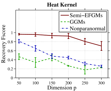
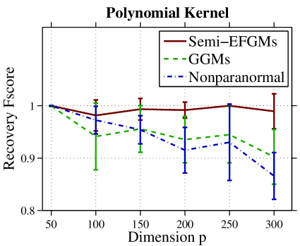
Figure 5.1: Support recovery F-score results on data model 1.

We now describe in detail these observations. Figure 5.1 shows the support recovery F-scores on data model 1. From the left panel we can see that Semi-EFGMs work significantly better than the other two considered methods when the mutual interactions of variables are modeled by heat kernel function. In this case, we also observe that Nonparanormal is much more accurate than GGMs in structure recovery. When polynomial kernel function is used to define mutual sufficient statistics (see right panel), Semi-EFGMs is slightly better than the two considered methods when $p<=100$ and the gap becomes more and more apparent as $p$ increases. The advantage of Semi-EFGMs is as expected because this approach explicitly models the nonlinear pairwise interactions which is hard to be captured by the traditional GGMs and Nonparanormals. Figure 5.2 shows the support recovery F-scores on data model 2 with different configurations of kernel function and sparsity level. From the left column we observe again that Semi-EFGMs significantly outperform the other two considered methods on heat kernel based models. From the right column we can see that on polynomial kernel based models, our model is significantly better than the other two considered methods when the graph structure is extremely sparse (i.e., $P=0.02$) while it is slightly better than the other two considered methods when the graph structure becomes less sparse (i.e., $P=0.05,0.1$). The numerical figures to generate Figure 5.1 and 5.2 are listed in Table 5.1. To visually inspect the support recovery performance of different methods, we show in Figure 5.3 several selected heatmaps reflecting the percentage of each graph matrix entry being identified as a nonzero element. Visual inspection on these heatmaps confirm that Semi-EFGMs perform favorably in graph structure recovery, especially when heat kernels are used as pairwise sufficient statistics (see the top two rows).

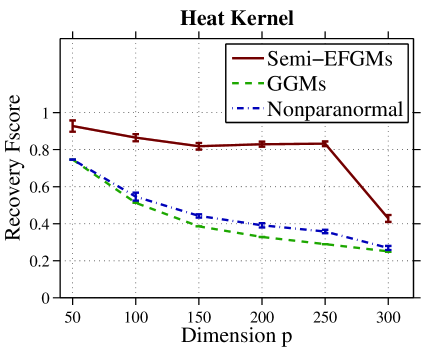
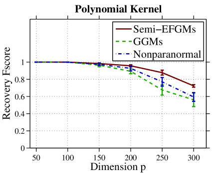
(a) Sparsity $P=0.02$

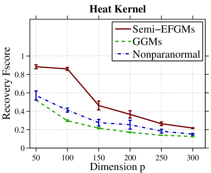
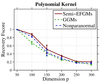
(b) Sparsity $P=0.05$

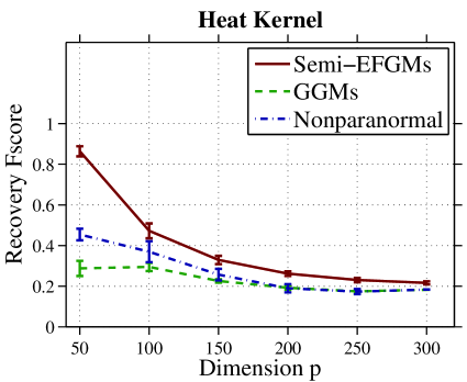
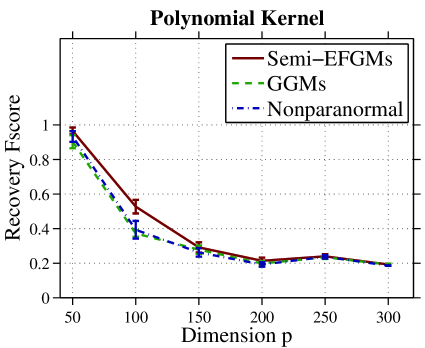
(c) Sparsity $P=0.1$

Figure 5.2: Support recovery F-score results on data model 2.

Table 5.1: Comparison of average (SE) of F-score for synthetic data over 100 replications.

Methods	$p=50$	$100$	$150$	$200$	$250$	$300$
Data model 1 with heat kernel
Semi-EFGMs	0.97 ($0.02$)	0.96 (0.04)	0.93 (0.05)	0.93 (0.06)	0.81 (0.07)	0.71 (0.10)
GGMs	0.47 (0.06)	0.34 (0.11)	0.44 (0.06)	0.27 (0.01)	0.18 (0.09)	0.23 (0.01)
Nonparanormal	0.81 (0.04)	0.65 (0.06)	0.48 (0.05)	0.45 (0.03)	0.32 (0.03)	0.26 (0.02)
Data model 1 with polynomial kernel
Semi-EFGMs	1.00 ($0.00$)	0.98 (0.03)	0.99 (0.02)	0.99 (0.02)	1.00 (0.00)	0.99 (0.03)
GGMs	0.99 (0.01)	0.94 (0.06)	0.96 (0.04)	0.94 (0.04)	0.94 (0.05)	0.90 (0.05)
Nonparanormal	1.00 (0.00)	0.97 (0.03)	0.95 (0.03)	0.92 (0.04)	0.93 (0.07)	0.87 (0.04)
Data model 2 with heat kernel, sparsity $P=0.02$
Semi-EFGMs	0.93 ($0.03$)	0.86 (0.02)	0.82 (0.02)	0.83 (0.01)	0.83 (0.01)	0.43 (0.02)
GGMs	0.75 (0.01)	0.51 (0.01)	0.39 (0.01)	0.33 (0.01)	0.29 (0.01)	0.25 (0.01)
Nonparanormal	0.75 (0.01)	0.55 (0.02)	0.44 (0.01)	0.39 (0.01)	0.36 (0.01)	0.27 (0.01)
Data model 2 with polynomial kernel, sparsity $P=0.02$
Semi-EFGMs	1.00 ($0.00$)	0.99 (0.01)	0.98 (0.01)	0.96 (0.01)	0.88 (0.03)	0.72 (0.02)
GGMs	1.00 (0.00)	0.99 (0.01)	0.96 (0.02)	0.89 (0.03)	0.68 (0.06)	0.56 (0.08)
Nonparanormal	1.00 (0.00)	0.99 (0.01)	0.97 (0.01)	0.93 (0.03)	0.77 (0.05)	0.59 (0.05)
Data model 2 with heat kernel, sparsity $P=0.05$
Semi-EFGMs	0.88 ($0.02$)	0.86 (0.02)	0.46 (0.05)	0.37 (0.04)	0.26 (0.02)	0.22 (0.01)
GGMs	0.52 (0.01)	0.30 (0.01)	0.22 (0.01)	0.17 (0.01)	0.14 (0.01)	0.13 (0.01)
Nonparanormal	0.57 (0.05)	0.41 (0.02)	0.28 (0.03)	0.25 (0.05)	0.18 (0.02)	0.15 (0.01)
Data model 2 with polynomial kernel, sparsity $P=0.05$
Semi-EFGMs	1.00 ($0.00$)	0.88 (0.02)	0.51 (0.10)	0.35 (0.01)	0.21 (0.02)	0.21 (0.02)
GGMs	0.99 (0.01)	0.67 (0.04)	0.42 (0.07)	0.25 (0.02)	0.20 (0.01)	0.14 (0.05)
Nonparanormal	0.99 (0.01)	0.82 (0.01)	0.44 (0.08)	0.29 (0.03)	0.18 (0.01)	0.18 (0.02)
Data model 2 with heat kernel, sparsity $P=0.1$
Semi-EFGMs	0.86 ($0.02$)	0.47 (0.04)	0.33 (0.02)	0.26 (0.01)	0.23 (0.01)	0.22 (0.01)
GGMs	0.29 (0.04)	0.29 (0.02)	0.23 (0.01)	0.19 (0.01)	0.17 (0.01)	0.18 (0.01)
Nonparanormal	0.45 (0.03)	0.37 (0.05)	0.26 (0.03)	0.19 (0.02)	0.17 (0.01)	0.18 (0.01)
Data model 2 with polynomial kernel, sparsity $P=0.1$
Semi-EFGMs	0.97 (0.02)	0.53 (0.04)	0.29 (0.03)	0.21 (0.02)	0.24 (0.01)	0.19 (0.01)
GGMs	0.90 (0.04)	0.37 (0.02)	0.28 (0.02)	0.20 (0.02)	0.23 (0.01)	0.19 (0.01)
Nonparanormal	0.93 (0.03)	0.39 (0.05)	0.26 (0.02)	0.19 (0.01)	0.24 (0.01)	0.19 (0.01)

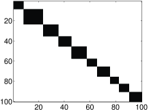
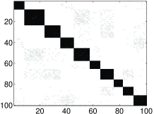
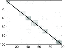
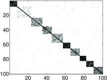
(a) Data model 1 with heat kernel, $p=100$

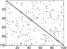
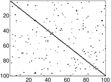
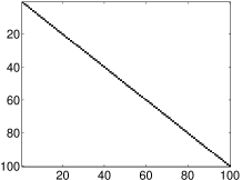
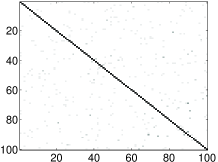
(b) Data model 2 ($P=0.02$) with heat kernel, $p=100$

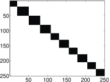
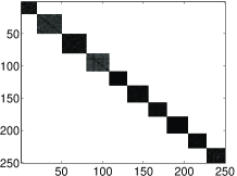
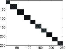
(c) Data model 1 with polynomial kernel, $p=250$

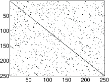
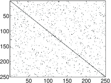
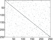
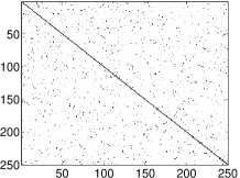
(d) Data model 2 ($P=0.02$) with polynomial kernel, $p=250$

Figure 5.3: Heatmaps of the frequency of nonzeros identified for each entry of the graph matrix out of 10 replications. White indicates 10 zeros identified out of 10 runs, and black indicates 0/10. For each row, from left to right: Ground truth, Semi-EFGMs, GGMs, Nonparanormal.

5.3 Stock Price Data

We further study the performance of Semi-EFGMs on a stock price data. This data contains the historical prices of S&P500 stocks over 5 years, from January 1, 2008 to January 1, 2013. By taking out the stocks with less than 5 years of history, we end up with 465 stocks, each having daily closing prices over 1,260 trading days. The prices are first adjusted for dividends and splits and the used to calculate daily log returns. Each day’s return can be represented as a point in $\mathbb{R}^{465}$. To apply Semi-EFGMs to this data, we use the polynomial kernel $\phi(X_{s},X_{t})=(\beta+\varphi(X_{s})^{\top}\varphi(X_{t}))^{\alpha}$ to model the pairwise interactions between stocks. The feature vector $\varphi(X_{s})$ is defined as the $5$-day prices of each stock (thus the number of samples reduces to $n=252$). Since the category information of S&P500 is available, we measure the performance by precision, recall and F-score of the top $k$ links (edges) on the constructed graph. A link is regarded as true if and only if it connects two nodes belonging to the same category. Note that the category information is not used in any of the graphical model learning procedures. The parameters $\alpha$, $\beta$ and $\lambda_{n}$ are tuned with cross-validation. Figure 5.4 shows the curves of precision, recall and F-score as functions of $k$. It can be seen that Semi-EFGMs significantly outperform the GGMs and Nonparanormal for identifying correct category links. This result suggests that the interactions among the S&P500 stocks is potentially highly nonlinear. We can also observe from Figure 5.4 that Nonparanormal is comparable or slightly inferior to GGMs on this data.

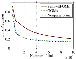
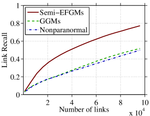
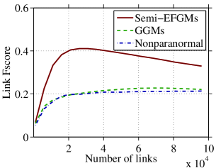
Figure 5.4: Category link Precision, Recall and F-score curves of the considered methods on the stock data S&P500.

6 Conclusion

In this paper, we propose Semi-EFGMs as a novel class of semiparametric exponential family graphical models. The main idea is to use a parametric nonlinear mapping families, e.g., Mercer kernels, to compute pairwise sufficient statistics. This allows us to capture complex interactions among variables which are not uncommon in modern engineering applications. We investigate two types of estimators, an $\ell_{1}$-regularized joint MLE estimator and an $\ell_{1}$-regularized node-conditional MLE estimator, for model parameters learning. Theoretically, we prove that under proper conditions, our proposed estimators are consistent in parameter estimation and the rates of convergence are optimal. Computationally, we show that with proper relaxations, the proposed estimators can be efficiently optimized via off-the-shelf GGMs solvers. Empirically, we demonstrate the advantage of Semi-EFGMs over the state-of-the-art parametric/semiparametric methods when applied to synthetic and real data. To conclude, Semi-EFGMs are statistically and computationally suitable for learning pairwise graphical models with nonlinear sufficient statistics. In the current model, we assume that the bivariate mapping $\phi$ is known up to the tunable parameters. In future work, we will investigate a more general model where $\phi$ admits a linear combination of basis functions, e.g., over RKHS, so that the sufficient statistics can be automatically learned in a data-driven fashion.

Appendix A Proofs of Lemmas

A.1 Proof of Lemma 1

Proof.

Since $X^{(i)}$ are i.i.d. samples of $X$, we have that $Z_{st}^{(i)}=\phi(X^{(i)}_{s},X^{(i)}_{t})-\mathbb{E}_{\theta^{*}}[\phi(X_{s},X_{t})]$ are also i.i.d. samples of $Z_{st}$. We use the exponential Markov inequality for the sum $Z=\sum_{i=1}^{n}Z_{st}^{(i)}$ and with a parameter $\eta>0$

$$\mathbb{P}\left(Z>\epsilon\right)=\mathbb{P}\left(\exp\{\eta Z\}>\exp\{\eta\epsilon\}\right)\leq\frac{\mathbb{E}[\exp\{\eta Z\}]}{\exp\{\eta\epsilon\}}=\frac{\prod_{i=1}^{n}\mathbb{E}\left[\exp\left\{\eta Z^{(i)}_{st}\right\}\right]}{\exp\{\eta\epsilon\}}.$$

If $\eta\leq\zeta$, Assumption 1 yields

$$\mathbb{P}\left(Z>n\varepsilon\right)\leq\frac{\exp\left\{n\sigma^{2}\eta^{2}/2\right\}}{\exp\{\eta n\varepsilon\}}=\exp\left\{-\eta n\varepsilon+n\sigma^{2}\eta^{2}/2\right\},$$

whose minimum is attained at $\eta=\min\left(\frac{\varepsilon}{\sigma^{2}},\zeta\right)$. Thus, for any $\varepsilon\leq\sigma^{2}\zeta$, we have

$$\mathbb{P}\left(Z>n\varepsilon\right)\leq\exp\left\{-\frac{n\varepsilon^{2}}{2\sigma^{2}}\right\}.$$

Repeating this argument for $-Z^{(i)}_{st}$ instead of $Z^{(i)}_{st}$, we obtain the same bound for $\mathbb{P}(-Z>n\varepsilon)$. Combining these two bounds yields

$$\mathbb{P}\left(\left|\frac{1}{n}\sum_{i=1}^{n}\phi(X^{(i)}_{s},X^{(i)}_{t})-\mathbb{E}_{\theta^{*}}[\phi(X_{s},X_{t})]\right|>\varepsilon\right)=\mathbb{P}\left(|Z|>n\varepsilon\right)\leq 2\exp\left\{-\frac{n\varepsilon^{2}}{2\sigma^{2}}\right\}.$$

This completes the proof. ∎

A.2 Proof of Lemma 2

Proof.

From the gradient term (3.2) and Lemma 1 we have that for any index pair $(s,t)$ and $\varepsilon<\sigma^{2}\zeta$

$$\mathbb{P}\left(\left|\frac{\partial L(\theta^{*};\mathbb{X}_{n})}{\partial\theta^{*}_{st}}\right|>\varepsilon\right) = \mathbb{P}\left(\left|\frac{1}{n}\sum_{i=1}^{n}\phi(X^{(i)}_{s},X^{(i)}_{t})-\mathbb{E}_{\theta^{*}}[\phi(X_{s},X_{t})]\right|>\varepsilon\right)\leq 2\exp\left\{-\frac{n\varepsilon^{2}}{2\sigma^{2}}\right\}.$$

By the union bound we obtain

$$\mathbb{P}(\|\nabla L(\theta^{*};\mathbb{X}_{n}))\|_{\infty}>\varepsilon) \leq 2p^{2}\exp\left\{-\frac{n\varepsilon^{2}}{2\sigma^{2}}\right\}.$$

Let us choose $\varepsilon=\sigma\sqrt{6\ln p/n}$. Since $n>6\ln p/(\sigma^{2}\zeta^{2})$, we have $\varepsilon<\sigma^{2}\zeta$. Therefore we obtain that with probability at least $1-2p^{-1}$,

$$\|\nabla L(\theta^{*};\mathbb{X}_{n})\|_{\infty}\leq\sigma\sqrt{6\ln p/n}.$$

This completes the proof. ∎

A.3 Proof of Lemma 3

Proof.

Let $\Delta\theta=\hat{\theta}_{n}-\theta^{*}$ and we define $\Delta\tilde{\theta}=t\Delta\theta$ where we pick $t=1$ if $\|\Delta\theta\|<r$ and $t\in(0,1)$ with $\|\Delta\tilde{\theta}\|=r$ otherwise. By definition, we have $\|\Delta\tilde{\theta}\|<r$. We now claim that $\|\Delta\tilde{\theta}_{\bar{S}}\|_{1}\leq 3\|\Delta\tilde{\theta}_{S}\|_{1}$. Indeed, since $\theta^{*}_{\bar{S}}=0$, we have

$$\|\theta^{*}+\Delta\tilde{\theta}\|_{1}-\|\theta^{*}\|_{1}=\|(\theta^{*}+\Delta\tilde{\theta})_{S}\|_{1}+\|\Delta\tilde{\theta}_{\bar{S}}\|_{1}-\|\theta^{*}_{S}\|_{1}\geq\|\Delta\tilde{\theta}_{\bar{S}}\|_{1}-\|\Delta\tilde{\theta}_{S}\|_{1}.$$ (A.1)

From the convexity of function $L(\theta;\mathbb{X}_{n})$ and $\lambda\geq 2\gamma_{n}=2\|\nabla L(\theta^{*};\mathbb{X}_{n})\|_{\infty}$ we have

$$L(\theta^{*}+\Delta\tilde{\theta};\mathbb{X}_{n})-L(\theta^{*};\mathbb{X}_{n})\geq\langle\nabla L(\theta^{*};\mathbb{X}_{n}),\Delta\tilde{\theta}\rangle\geq-\|\nabla L(\theta^{*};\mathbb{X}_{n})\|_{\infty}\|\Delta\tilde{\theta}\|_{1}\geq-\frac{\lambda_{n}}{2}\|\Delta\tilde{\theta}\|_{1}.$$ (A.2)

Due to the optimality of $\hat{\theta}_{n}$ and the convexity of $L(\theta;\mathbb{X}_{n})$, it holds that

$$L(\theta^{*}+\Delta\tilde{\theta};\mathbb{X}_{n})+\lambda_{n}\|\theta^{*}+\Delta\tilde{\theta}\|_{1}\leq L(\theta^{*};\mathbb{X}_{n})+\lambda_{n}\|\theta^{*}\|_{1}.$$ (A.3)

By combining the proceeding three inequalities (A.1), (A.2) and (A.3), we obtain that

$$0 \geq L(\theta^{*}+\Delta\tilde{\theta};\mathbb{X}_{n})+\lambda_{n}\|\theta^{*}+\Delta\tilde{\theta}\|_{1}-L(\theta^{*};\mathbb{X}_{n})-\lambda_{n}\|\theta^{*}\|_{1}$$

$$\geq -\frac{\lambda_{n}}{2}(\|\Delta\tilde{\theta}_{S}\|_{1}+\|\Delta\tilde{\theta}_{\bar{S}}\|_{1})+\lambda_{n}(\|\Delta\tilde{\theta}_{\bar{S}}\|_{1}-\|\Delta\tilde{\theta}_{S}\|_{1}),$$

which implies $\|\Delta\tilde{\theta}_{\bar{S}}\|_{1}\leq 3\|\Delta\tilde{\theta}_{S}\|_{1}$. From second-order Taylor expansion we know that there exists a real number $\xi\in[0,1]$ such that

$$L(\theta^{*}+\Delta\tilde{\theta};\mathbb{X}_{n})=L(\theta^{*};\mathbb{X}_{n})+\langle\nabla L(\theta^{*};\mathbb{X}_{n}),\Delta\tilde{\theta}\rangle+\frac{1}{2}\tilde{\Delta}\theta^{\top}\nabla^{2}L(\theta^{*}+\xi\Delta\tilde{\theta};\mathbb{X}_{n})\tilde{\Delta}\theta.$$

By using Assumption 2 (note that $\|\xi\tilde{\Delta}\theta\|\leq\|\tilde{\Delta}\theta\|<r$) and (A.2) we have

$$L(\theta^{*}+\Delta\tilde{\theta};\mathbb{X}_{n})-L(\theta^{*};\mathbb{X}_{n})\geq\langle\nabla L(\theta^{*};\mathbb{X}_{n}),\Delta\tilde{\theta}\rangle+\frac{\beta}{2}\|\tilde{\Delta}\theta\|^{2}\geq-\frac{\lambda_{n}}{2}\|\Delta\tilde{\theta}\|_{1}+\frac{\beta}{2}\|\tilde{\Delta}\theta\|^{2}.$$ (A.4)

By combining the inequalities (A.1), (A.3) and (A.4), we obtain that

$$0 \geq L(\theta^{*}+\Delta\tilde{\theta};\mathbb{X}_{n})+\lambda_{n}\|\theta^{*}+\Delta\tilde{\theta}\|_{1}-L(\theta^{*};\mathbb{X}_{n})-\lambda_{n}\|\theta^{*}\|_{1}$$

$$\geq -\frac{\lambda_{n}}{2}\|\Delta\tilde{\theta}\|_{1}+\frac{\beta}{2}\|\tilde{\Delta}\theta\|^{2}+\lambda_{n}(\|\tilde{\Delta}\theta_{\bar{S}}\|_{1}-\|\tilde{\Delta}\theta_{S}\|_{1})$$

$$\geq \frac{\lambda_{n}}{2}(\|\Delta\tilde{\theta}_{\bar{S}}\|_{1}-3\|\Delta\tilde{\theta}_{S}\|_{1})+\beta\|\Delta\tilde{\theta}\|^{2}$$

$$\geq -1.5\lambda_{n}\|\Delta\tilde{\theta}_{S}\|_{1}+\beta\|\Delta\tilde{\theta}\|^{2}\geq-1.5\lambda_{n}\sqrt{|S|}\|\Delta\tilde{\theta}\|+\beta\|\Delta\tilde{\theta}\|^{2},$$

which implies that

$$\|\Delta\tilde{\theta}\|\leq 1.5\lambda_{n}\beta^{-1}\sqrt{\|\theta^{*}\|_{0}}\leq 1.5c_{0}\sqrt{\|\theta^{*}\|_{0}}\beta^{-1}\gamma_{n}=\gamma.$$

Since $\gamma<r$, we claim that $t=1$ and thus $\Delta\tilde{\theta}=\Delta\theta$. Indeed, if otherwise $t<1$, then $\|\Delta\tilde{\theta}\|=r>\gamma$ which contradicts the above inequality. This completes the proof. ∎

A.4 Proof of Lemma 4

Proof.

Note that for any $\eta$, $\exp\{\eta x\}$ is convex with respect to $x$. By applying Jensen’s inequality we have

$$\exp\left\{\eta\mathbb{E}_{\theta^{*}_{s}}[\phi(X_{s},X_{t})\mid X_{\setminus s}]\right\}\leq\mathbb{E}_{\theta^{*}_{s}}[\exp\left\{\eta\phi(X_{s},X_{t})\right\}\mid X_{\setminus s}].$$

By taking the expectation $\mathbb{E}_{\theta^{*}_{\setminus s}}[\cdot]$ with respect to the marginal distribution of $X_{\setminus s}$, and using the rule of iterated expectation, we obtain

$$\mathbb{E}_{\theta^{*}_{\setminus s}}\left[\exp\left\{\eta\mathbb{E}_{\theta^{*}_{s}}[\phi(X_{s},X_{t})\mid X_{\setminus s}]\right\}\right]\leq\mathbb{E}_{\theta^{*}_{\setminus s}}\left[\mathbb{E}_{\theta^{*}_{s}}[\exp\left\{\eta\phi(X_{s},X_{t})\right\}\mid X_{\setminus s}]\right]=\mathbb{E}_{\theta^{*}}[\exp\{\eta\phi(X_{s},X_{t})\}].$$

By using the “law of the unconscious statistician” and the above inequality we obtain

$$\mathbb{E}[\exp\{\eta\tilde{Z}_{st}\}]\leq\mathbb{E}[\exp\{\eta Z_{st}\}]\leq\exp\left\{\sigma^{2}\eta^{2}/2\right\},$$

where the last inequality follows from Assumption 1. This completes the proof. ∎

A.5 Proof of Lemma 6

Proof.

Recall the formulation of gradient $\nabla\tilde{L}(\theta_{s};\mathbb{X}_{n})$ in (3.6). For any node $t\in V\setminus s$, we have

$$\left|\frac{\partial\tilde{L}(\theta_{s};\mathbb{X}_{n})}{\partial\theta_{st}}\right|$$

$$= \left|\frac{1}{n}\sum_{i=1}^{n}-\phi(X^{(i)}_{s},X^{(i)}_{t})+\mathbb{E}_{\theta^{*}_{s}}[\phi(X_{s},X^{(i)}_{t})\mid X^{(i)}_{\setminus s}]\right|$$

$$\leq \left|\frac{1}{n}\sum_{i=1}^{n}\phi(X^{(i)}_{s},X^{(i)}_{t})-\mathbb{E}_{\theta^{*}}[\phi(X_{s},X_{t})]\right|+\left|\frac{1}{n}\sum_{i=1}^{n}\mathbb{E}_{\theta^{*}_{s}}[\phi(X_{s},X^{(i)}_{t})\mid X^{(i)}_{\setminus s}]-\mathbb{E}_{\theta^{*}}[\phi(X_{s},X_{t})]\right|.$$

Therefore, for any $\varepsilon\leq 2\sigma^{2}\zeta$,

$$\mathbb{P}\left(\left|\frac{\partial\tilde{L}(\theta_{s};\mathbb{X}_{n})}{\partial\theta_{st}}\right|>\varepsilon\right) \leq \mathbb{P}\left(\left|\frac{1}{n}\sum_{i=1}^{n}\phi(X^{(i)}_{s},X^{(i)}_{t})-\mathbb{E}_{\theta^{*}}[\phi(X_{s},X_{t})]\right|>\frac{\varepsilon}{2}\right)$$

$$+\mathbb{P}\left(\left|\frac{1}{n}\sum_{i=1}^{n}\mathbb{E}_{\theta^{*}_{s}}[\phi(X_{s},X^{(i)}_{t})\mid X^{(i)}_{\setminus s}]-\mathbb{E}_{\theta^{*}}[\phi(X_{s},X_{t})]\right|>\frac{\varepsilon}{2}\right)$$

$$\leq 4\exp\left\{-\frac{n\varepsilon^{2}}{8\sigma^{2}}\right\},$$

where the last “$\leq$” follows from Lemma 1 and Lemma 5. By the union bound we obtain

$$\mathbb{P}(\|\nabla\tilde{L}(\theta^{*}_{s};\mathbb{X}_{n})\|_{\infty}>\varepsilon) \leq 4p\exp\left\{-\frac{n\varepsilon^{2}}{8\sigma^{2}}\right\}.$$

Let us choose $\varepsilon=2\sigma\sqrt{6\ln p/n}$. Since $n>6\ln p/(\sigma^{2}\zeta^{2})$, we have $\varepsilon<2\sigma^{2}\zeta$. We conclude that with probability at least $1-4p^{-2}$,

$$\|\nabla\tilde{L}(\theta^{*}_{s};\mathbb{X}_{n})\|_{\infty}\leq 2\sigma\sqrt{6\ln p/n}.$$

This proves the desired bound. ∎

References

• Acemoglu (2009) Acemoglu, D. The crisis of 2008: Lessons for and from economics. Critical Review, 21:185–194, 2009.
• Bach & Jordan (2002) Bach, F.R. and Jordan, M.I. Learning graphical models with mercer kernels. In Proceedings of the 16th Annual Conference on Neural Information Processing Systems (NIPS’02), 2002.
• Banerjee et al. (2008) Banerjee, O., Ghaoui, L. El, and d Aspremont, A. Model selection through sparse maximum likelihood estimation for multivariate gaussian or binary data. Journal of Machine Learning Research, 9:485–516, 2008.
• Baraniuk et al. (2008) Baraniuk, R. G., Davenport, M., DeVore, R. A., and Wakin, M. A simple proof of the restricted isometry property for random matrices. Constructive Approximation, 28(3):253–263, 2008.
• Beck & Teboulle (2009) Beck, A. and Teboulle, Marc. A fast iterative shrinkage-thresholding algorithm for linear inverse problems. SIAM J. Imaging Sci., 2(1):183–202, 2009.
• Bishop (2006) Bishop, C.M. Pattern Recognition and Machine Learning. Springer-Verlag New York, Inc., Secaucus, NJ, USA, 2006. ISBN 978-0-387-31073-2.
• Bishop et al. (2007) Bishop, Y., Fienberg, S., and Holland, P. Discrete Multivariate Analysis: Theory and Practice. Springer Verlag New York, Inc., 2007. ISBN 978-0-387-72806-3.
• Cai et al. (2011) Cai, T., liu, W., and Luo, X. A constrained $\ell_{1}$ minimization approach to sparse precision matrix estimation. Journal of the American Statistical Association, 106(494):594–607, 2011.
• Candès et al. (2011) Candès, E. J., Eldarb, Y. C., Needella, D., and Randallc, P. Compressedsensing with coherent and redundantdictionarie. Applied and Computational Harmonic Analysis, 31(1):59–73, 2011.
• Clifford (1990) Clifford, P. Markov random fields in statistics. In Grimmett, G. and Welsh, D. J. A. (eds.), Disorder in physical systems. Oxford Science Publications, 1990.
• d’Aspremont et al. (2008) d’Aspremont, A., Banerjee, O., and Ghaoui, L. First-order methods for sparse covariance selection. SIAM Journal on Matrix Analysis and its Applications, 30(1):56–66, 2008.
• Dobra & Lenkoski (2011) Dobra, A. and Lenkoski, A. Copula gaussian graphical models and their application to modeling functional disability data. The Annals of Applied Statistics, 5:969–993, 2011.
• Friedman et al. (2008) Friedman, J., Hastie, T., and Tibshirani, R. Sparse inverse covariance estimation with the graphical lasso. Biostatistics, 9(3):432–441, 2008.
• Gu et al. (2013) Gu, Chong, Jeon, Yongho, and Lin, Yi. Nonparametric density estimation in high-dimensions. Statistica Sinica, 23:1131–1153, 2013.
• Jalali et al. (2011) Jalali, A., Ravikumar, P., Vasuki, V., and Sanghavi., S. On learning discrete graphical models using group-sparse regularization. In Proceedings of the Fourteenth International Conference on Artificial Intelligence and Statistics (AISTATS’11), pp.  378–387, 2011.
• Klaassen & Wellner (1997) Klaassen, C. A. J. and Wellner, J. A. Efficient estimation in the bivariate normal copula model: Normal margins are least-favorable. Bernoulli, 3:55–77, 1997.
• Lafferty et al. (2012) Lafferty, J., Liu, H., and Wasserman, L. Sparse nonparametric graphical models. Statistical Science, 27(4):519–537, 2012.
• Lauritzen (1996) Lauritzen, S. Graphical models. Oxford University Press, 1996.
• Liu et al. (2009) Liu, H., Lafferty, J., and Wasserman, L. The nonparanormal: Semiparametric estimation of high dimensional undirected graphs. Journal of Machine Learning Research, 10:2295–2328, 2009.
• Liu et al. (2012) Liu, H., Han, F., Yuan, M., Lafferty, J., and Wasserman, L. High dimensional semiparametric gaussian copula graphical models. Annals of Statistics, 40(4):2293–2326, 2012.
• Lu (2009) Lu, Z. Smooth optimization approach for sparse covariance selection. SIAM Journal on Optimization, 19(4):1807–1827, 2009.
• Meinshausen & Bühlmann (2006) Meinshausen, N. and Bühlmann, P. High-dimensional graphs and variable selection with the lasso. Annals of Statistics, 34(3):1436–1462, 2006.
• Negahban et al. (2012) Negahban, S. N., Ravikumar, P., Wainwright, M. J., and Yu, B. A unified framework for high-dimensional analysis of m-estimators with decomposable regularizers. Statistical Science, 27(4):538–557, 2012.
• Nesterov (2005) Nesterov, Yu. Smooth minimization of non-smooth functions. Mathematical Programming, 103(1):127–152, 2005.
• Ravikumar et al. (2010) Ravikumar, P., Wainwright, M.J., and Lafferty, J. High-dimensional ising model selection using l1-regularized logistic regression. Annals of Statistics, 38(3):1287–1319, 2010.
• Ravikumar et al. (2011) Ravikumar, P., Wainwright, M. J., Raskutti, G., and Yu, B. High-dimensional covariance estimation by minimizing $\ell_{1}$-penalized log-determinant divergence. Electronic Journal of Statistics, 5:935–980, 2011.
• Rijsbergen (1979) Rijsbergen, C.J. Van. Information Retrieval (2nd ed.). Butterworth-Heinemann, Newton, MA, USA, 1979. ISBN 0408709294.
• Rothman et al. (2008) Rothman, A. J., Bickel, P. J., Levina, E., and Zhu, J. Sparse permutation invariant covariance estimation. Electronic Journal of Statistics, 2:494–515, 2008.
• Schmidt et al. (2009) Schmidt, M., Berg, E.V.D., Friedlander, M.P., and Murphy, K. Optimizing costly functions with simple constraints: A limited-memory projected quasi-newton algorithm. In Proceedings of the Twelfth International Conference on Artificial Intelligence and Statistics (AISTATS’09), pp.  456–463, 2009.
• Speed & Kiiveri (1986) Speed, T. P. and Kiiveri, H. T. Gaussian markov distributions over finite graphs. Annals of Statistics, 14:138–150, 1986.
• Tseng (2008) Tseng, P. On accelerated proximal gradient methods for convex-concave optimization. submitted to SIAM Journal of Optimization, 2008.
• Tsukahara (2005) Tsukahara, H. Semiparametric estimation in copula models. Canadian Journal of Statistics, 33:357–375, 2005.
• Vershynin (2011) Vershynin, Roman. Introduction to the non-asymptotic analysis of random matrices. 2011. URL http://arxiv.org/pdf/1011.3027.pdf.
• Wainwright & Jordan (2008) Wainwright, M.J. and Jordan, M.I. Graphical models, exponential families, and variational inference. Foundations and Trends in Machine Learning, 1(1-2):1–305, 2008.
• Wang et al. (2010) Wang, C., Sun, D., and Toh, K.-C. Solving log-determinant optimization problems by a newton-cg primal proximal point algorithm. SIAM Journal on Optimization, 20:2994–3013, 2010.
• Xue & Zou (2012) Xue, L. and Zou, H. Regularized rank-based estimation of high-dimensional nonparanormal graphical models. Annals of Statistics, 40(5):2541–2571, 2012.
• Yang et al. (2012) Yang, E., Ravikumar, P., Allen, G. I., and Liu, Z. Graphical models via generalized linear models. In Proceedings of the 26th Annual Conference on Neural Information Processing Systems (NIPS’12), 2012.
• Yang et al. (2013) Yang, E., Ravikumar, P., Allen, G. I., and Liu, Z. On graphical models via univariate exponential family distributions. 2013. URL http://arxiv.org/pdf/1301.4183v1.pdf.
• Yuan (2010) Yuan, M. High dimensional inverse covariance matrix estimation via linear programming. Journal of Machine Learning Research, 11:2261–2286, 2010.
• Yuan & Lin (2007) Yuan, M. and Lin, Y. Model selection and estimation in the gaussian graphical model. Biometrika, 94(1):19–35, 2007.
• Yuan (2012) Yuan, X. Alternating direction method of multipliers for covariance selection models. Journal of Scientific Computing, 2012.
• Yuan & Yan (2013) Yuan, X.-T. and Yan, S. Forward basis selection for pursuing sparse representations over a dictionary. IEEE Transactions on Pattern Analysis and Machine Intelligence, to appear, 2013.
• Zhang & Zhang (2012) Zhang, C.-H. and Zhang, T. A general framework of dual certificate analysis for structured sparse recovery problems. 2012. URL http://arxiv.org/pdf/1201.3302v2.pdf.