Phase diagram of the square lattice bilayer Hubbard model: a variational Monte Carlo study

Abstract

We investigate the phase diagram of the square lattice bilayer Hubbard model at half filling with the variational Monte Carlo method for both the magnetic and the paramagnetic case as a function of the interlayer hopping $t_{\perp}$ and on-site Coulomb repulsion $U$. With this study we resolve some discrepancies in previous calculations based on the dynamical mean field theory, and we are able to determine the nature of the phase transitions between metal, Mott insulator and band insulator. In the magnetic case we find only two phases: An antiferromagnetic Mott insulator at small $t_{\perp}$ for any value of $U$ and a band insulator at large $t_{\perp}$. At large $U$ values we approach the Heisenberg limit. The paramagnetic phase diagram shows at small $t_{\perp}$ a metal to Mott insulator transition at moderate $U$ values and a Mott to band insulator transition at larger $U$ values. We also observe a re-entrant Mott insulator to metal transition and metal to band insulator transition for increasing $t_{\perp}$ in the range of $5.5t<U<7.5t$. Finally, we discuss the obtained phase diagrams in relation to previous studies based on different many-body approaches.

1 Introduction

Understanding the origin of transitions from a metal to a Mott or a band insulator in correlated systems has been a topic of intensive debate in the past few years. Various generalizations of the Hubbard model have been investigated for this purpose, like the extended Hubbard model [1], the ionic Hubbard model in one and two dimensions [2, 3, 4, 5, 6], the two-band Hubbard model [7] and the bilayer Hubbard model [8, 9, 10, 11, 12, 13, 14, 15]. The latter has been specially important in relation to the bilayer high-$T_{c}$ cuprates [16, 17]. Previous investigations of the above models have been carried out primarily by employing dynamical mean-field theory (DMFT) [18] and its cluster extensions [19, 20, 21, 22, 23]. While DMFT already captures a significant amount of key properties in correlated systems, it is extremely important to analyse these models with completely unrelated many-body methods in order to get a deeper understanding of the underlying physics. In this work we investigate the phase diagram of the square lattice bilayer Hubbard model at half filling with the variational Monte Carlo (VMC) method. With this study (i) we are able to resolve some discrepancies between previous DMFT and cluster DMFT studies and (ii) we find new aspects of the Mott to band transition not captured in previous studies.

The bilayer Hubbard model on the square lattice is given by the following Hamiltonian:

$$\hat{H} =\hat{H}_{t}+\hat{H}_{t_{\perp}}+\hat{H}_{U}$$ (1)

$$\hat{H}_{t} =-t\sum_{l,\sigma}\sum_{\langle ij\rangle}\left(\hat{c}^{\dagger}_{j,l,\sigma}\hat{c}_{i,l,\sigma}^{\phantom{\dagger}}+\mathrm{h.c.}\right)$$ (2)

$$\hat{H}_{t_{\perp}} =-t_{\perp}\sum_{i,\sigma}\left(\hat{c}^{\dagger}_{i,2,\sigma}\hat{c}_{i,1,\sigma}^{\phantom{\dagger}}+\mathrm{h.c.}\right)$$ (3)

$$\hat{H}_{U} =U\sum_{i,l}\hat{n}_{i,l,\uparrow}\hat{n}_{i,l,\downarrow}\,.$$ (4)

Here $\hat{c}^{\dagger}_{i,l,\sigma}$ ($\hat{c}^{\phantom{\dagger}}_{i,l,\sigma}$) denotes the creation (annihilation) operator of one electron on site $i$ and plane $l\in\{1,2\}$ with spin $\sigma\in\{\uparrow,\downarrow\}$, while $\hat{n}_{i,l,\sigma}=\hat{c}^{\dagger}_{i,l,\sigma}\hat{c}^{\phantom{\dagger}}_{i,l,\sigma}$ is the electron density. $t$ is the nearest neighbour hopping parameter in the plane, $t_{\perp}$ denotes the hopping between planes and $U$ is the on-site Coulomb repulsion, see figure 1.

    

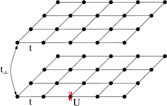
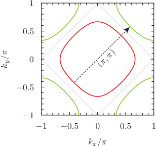
Figure 1: Left: Illustration of the bilayer Hubbard model. Right: Fermi surfaces of the bonding (green) and antibonding (red) band for the square lattice bilayer with nearest neighbour hopping for $t_{\perp}/t$=1. The symmetry of the dispersion relation ensures a perfect Fermi surface nesting between the bands as long as $t_{\perp}<4$. The grey curve is the Fermi surface for $t_{\perp}=0$.

Note that in the following we measure all quantities in units of $t$. The $U=0$ dispersion,

$$\epsilon_{\mathbf{k}}^{\pm}=-2t\big{(}\cos(k_{x})+\cos(k_{y})\big{)}\pm t_{\perp},$$ (5)

for the bonding/antibonding ($\pm$) bands is at half filling perfectly nested, i.e. $\epsilon_{\mathbf{k}+\mathbf{Q}}^{\pm}=\epsilon_{\mathbf{k}}^{\mp}$ with $\mathbf{Q}=(\pi,\pi)$, as illustrated in figure 1. As a consequence, the ground state [24] is an ordered antiferromagnet for any $U>0$, as long as a Fermi surface exists, which is the case for $t_{\perp}/t<4$ in the limit $U\to 0$.

In this work we analyse the magnetic phase diagram at $T=0$ as well as the paramagnetic case, which we investigate by suppressing the long-range magnetic ordering. This latter investigation, while it is done at $T=0$, it is relevant for predictions at finite and small temperatures where long-range magnetic order is absent as a consequence of the Mermin-Wagner theorem [25].

In the limit of large interaction strength, $U\rightarrow\infty$, the Hubbard Hamiltonian in equation (1) reduces to the Heisenberg Hamiltonian,

$$\hat{H}=J\sum_{l}\sum_{\langle ij\rangle}\hat{\mathbf{S}}_{i,l}\cdot\hat{\mathbf{S}}_{j,l}+J_{\perp}\sum_{i}\hat{\mathbf{S}}_{i,1}\cdot\hat{\mathbf{S}}_{i,2}\,,\\$$ (6)

with $J={4t^{2}}/{U}$ and $J_{\perp}={4t_{\perp}^{2}}/{U}$. The bilayer Heisenberg Hamiltonian has itself been subject of extensive research, and it has been found to undergo an order-disorder transition [26] at $J_{\perp}/J=2.552$, which corresponds to $t_{\perp}/t=1.588$ in terms of the Hubbard Hamiltonian’s hopping parameters [27][28].

Studies of the complete phase diagram of the bilayer Hubbard model have been conducted by Fuhrmann et alusing DMFT [8] and by Kancharla and Okamoto with cluster DMFT [9]. The authors of reference [8] concentrated on the paramagnetic phase at finite temperature and found a metallic phase at small $U$ and small $t_{\perp}$ values as well as an insulating phase as $t_{\perp}$ increases (the band insulator) or $U$ increases (the Mott insulator), but no clear separation between the Mott and the band insulating phase was found.

The authors of reference [9] considered clusters of sizes $2\times 2$ (i.e. two sites per plane) within cluster DMFT and performed exact diagonalization calculations to solve the impurity problem, which allowed them to investigate $T=0$ and to obtain both a magnetic phase diagram as well as a $T=0$ phase diagram where magnetism is suppressed. These results show several important differences with respect to the earlier phase diagram by Fuhrmann et al [8]: First of all, Kancharla et al [9] distinguish between a Mott and a band insulator by looking at the behaviour of the charge gap as a function of $t_{\perp}$. Also, they find a Mott insulator at $t_{\perp}=0$ for any value of $U>0$, even if magnetism is suppressed. They mention the cluster DMFT’s intralayer spatial correlation as the reason for this being found with cluster DMFT but not in the DMFT results by Fuhrmann et al [8]. However, at $t_{\perp}=0$ the planes are completely decoupled and should have the same properties as a single plane. For the single plane, different methods predict that the system becomes a Mott insulator at some finite $U$, as shown for instance in reference [29], where the critical $U$ was calculated using the dynamical cluster approximation with a variety of cluster sizes. Also, Tocchio et al [30] and Capello et al [31] showed with the VMC method (which in the first reference includes Fermi-surface renormalization effects) the appearance of a Mott insulator at a finite $U$.

A possible reason for the occurrence of a Mott insulator for any finite $U$ in reference [9] might be the small cluster size of $2\times 2$ used in cluster DMFT. Having two sites in each plane breaks the fourfold rotational symmetry of the square lattice and results in an artificially enhanced local pair within each plane for any $U>0$. This can noticeably affect the phase diagram of a system, as reported by Lee et alfor the two-orbital Hubbard model [32]. A particularly interesting feature of the phase diagram in reference [9] is that for a certain range of $U$ values the system goes through two phase transitions as $t_{\perp}$ is increased, first from a Mott insulator to a metal and then from a metal to a band insulator, while at large $U$ the system exhibits a direct transition from a Mott to a band insulator. Analogous features have been also proposed in reference [3] for the ionic Hubbard model. If magnetic order is allowed, it is noteworthy that no magnetic ordering was found in the cluster DMFT [9] for small $U$ and $2\lesssim t_{\perp}<4$, even though there is a perfect nesting between the Fermi surfaces of the bonding and antibonding bands with $\mathbf{Q}=(\pi,\pi)$. A metallic phase at small $U$ in the magnetic phase diagram has been also obtained in a Determinant Quantum Monte Carlo (DQMC) study [10]. This result could be a consequence of the finite temperatures that have been used in DQMC, since they could be large enough to destroy the tiny magnetic order at small $U$, where the gap is exponentially small.

Overall, DMFT and previous DQMC results do not give a conclusive picture yet, making it worthwhile to also employ other methods in order to gain a deeper understanding of the physics in the bilayer Hubbard model.

2 Methods

The variational Monte Carlo method was introduced by McMillan in 1965 to calculate the ground state of liquid ⁴He [33], and in 1977 applied to a fermionic system for the first time [34]. Its basic idea is to use the Rayleigh-Ritz principle [35] to approximate the ground state through a variational many-body wavefunction. It is a Monte Carlo method because a stochastic sampling is used to evaluate the sum over a high dimensional configuration space. A detailed description of how the variational Monte Carlo method can be applied to the Hubbard model may be found for instance in reference [36]. The VMC approach has played also a central role when examining the large-$U$ limit of the Hubbard model [37, 38, 39], in the context of high-temperature superconductivity.

The choice of the variational many-body wavefunction is crucial in order to obtain reliable results. Here, we define a variational state $\ket{\Psi}$ that consists of two parts: A Slater determinant $\ket{\Phi}$ and a Jastrow correlator $\hat{\mathcal{P}}_{J}$ acting on $\ket{\Phi}$:

$$\ket{\Psi}=\hat{\mathcal{P}}_{J}\ket{\Phi}\,.$$ (7)

Here the Slater determinant $\ket{\Phi}$ ensures the antisymmetry of the wavefunction while the Jastrow factor $\hat{\mathcal{P}}_{J}$ modifies its amplitude to take into account electronic correlations.

The state $\ket{\Phi}$ is the ground state of a variational mean-field Hamiltonian $\hat{H}_{\mathrm{var}}$ which may include up to five different terms: Nearest neighbour hopping within the planes, hopping between the planes, superconducting pairing in the planes with $d$-wave symmetry, pairing between the planes and an antiferromagnetic term, according to the following equations [40, 41, 42]:

$$\hat{H}_{\mathrm{var}} =\hat{H}_{t}+\hat{H}^{\mathrm{(var)}}_{t_{\perp}}+\hat{H}_{\Delta}+\hat{H}_{\Delta_{\perp}}+\hat{H}_{\mathrm{mag}}$$ (8)

$$\ \hat{H}_{t} =-t\sum_{\mathbf{r},l}\left(\hat{c}^{\dagger}_{\mathbf{r}+\mathbf{e}_{x},l}+\hat{c}^{\dagger}_{\mathbf{r}-\mathbf{e}_{x},l}+\hat{c}^{\dagger}_{\mathbf{r}+\mathbf{e}_{y},l}+\hat{c}^{\dagger}_{\mathbf{r}-\mathbf{e}_{y},l}\right)\hat{c}_{\mathbf{r},l}$$ (9)

$$\ \hat{H}_{t_{\perp}}^{\mathrm{(var)}} =-t_{\perp}^{\mathrm{(var)}}\sum_{\mathbf{r}}\left(\hat{c}^{\dagger}_{\mathbf{r},2}\hat{c}_{\mathbf{r},1}^{\phantom{\dagger}}+\mathrm{h.c.}\right)$$ (10)

$$\ \hat{H}_{\Delta} =\Delta\sum_{\mathbf{r},l}\hat{c}^{\dagger}_{\mathbf{r},l,\uparrow}\Big{(}\hat{c}^{\dagger}_{\mathbf{r}+\mathbf{e}_{x},l,\downarrow}+\hat{c}^{\dagger}_{\mathbf{r}-\mathbf{e}_{x},l,\downarrow}-\hat{c}^{\dagger}_{\mathbf{r}+\mathbf{e}_{y},l,\downarrow}-\hat{c}^{\dagger}_{\mathbf{r}-\mathbf{e}_{y},l,\downarrow}\Big{)}+\mathrm{h.c.}$$ (11)

$$\ \hat{H}_{\Delta_{\perp}} =\Delta_{\perp}\sum_{\mathbf{r}}\left(\hat{c}^{\dagger}_{\mathbf{r},1,\uparrow}\hat{c}^{\dagger}_{\mathbf{r},2,\downarrow}+\hat{c}^{\dagger}_{\mathbf{r},2,\uparrow}\hat{c}^{\dagger}_{\mathbf{r},1,\downarrow}+\mathrm{h.c.}\right)$$ (12)

$$\ \hat{H}_{\mathrm{mag}} =\mu_{m}\sum_{i}(-1)^{\tau(i)}\hat{S}^{z}_{i}\,.$$ (13)

Here $\mathbf{r}$ labels the sites within the planes, $l$ is the plane index, $\mathbf{e}_{x(y)}$ is the unity vector along the $x(y)$ direction and $S^{z}_{i}$ indicates the $z$ component of the spin operator on site $i$. Note that the square lattice bilayer model is a bipartite lattice, with $\tau(i)\in\{1,2\}$ labelling the sublattice of site $i$, so that a different spin orientation is preferred for each of the two sublattices when $\mu_{m}>0$. We would like to mention that the following particle-hole transformation has been used in order to diagonalize the variational Hamiltonian:

$$\hat{c}_{i\uparrow}=\hat{d}_{i\uparrow}\qquad \mathrm{and}\qquad\hat{c}_{i\uparrow}^{\dagger}=\hat{d}_{i\uparrow}^{\dagger}$$ (14)

$$\hat{c}_{i\downarrow}=\hat{d}_{i\downarrow}^{\dagger}\qquad \mathrm{and}\qquad\hat{c}_{i\downarrow}^{\dagger}=\hat{d}_{i\downarrow}\,.$$ (15)

This is possible because we chose the spins to align along the $z$ direction in the antiferromagnetic term of Eq. (13).

The alternative choice of aligning the spins along the $x$ direction, see for instance reference [43], does not allow to study magnetism and pairing together as a single Slater determinant, but it is often preferred because the variational state is improved by the application of a spin-Jastrow factor $J_{s}=\exp\left(\frac{1}{2}\sum_{ij}u_{ij}S^{z}_{i}S^{z}_{j}\right)$ that couples spins in a direction orthogonal to the ordering one, see reference [44].

The Jastrow factor $\hat{\mathcal{P}}_{J}$ implements a long-range density-density correlation which has been shown to be essential in the variational description of Mott insulators [45]. In order to account for the bilayer nature of the system we used a modified version of the Jastrow factor with a different set of variational parameters for intraplane ($v$) and interplane ($v_{\perp}$) correlations:

$$\hat{\mathcal{P}}_{J}=\exp\left(\frac{1}{2}\sum_{ij}\sum_{l_{1},l_{2}}\left[v(ij)\delta_{l_{1},l_{2}}+v_{\perp}(ij)(1-\delta_{l_{1},l_{2}})\right]\;\hat{n}_{i,l_{1}}\hat{n}_{j,l_{2}}\right)\,,$$ (16)

with the $v(ij)$ and the $v_{\perp}(ij)$ being optimized independently for every distance $|\mathbf{r}_{i}-\mathbf{r}_{j}|$.

The Metropolis algorithm [46] with single particle updates has been used to generate the electronic configurations, while the optimization of the variational wavefunction was done using the stochastic reconfiguration method [47, 48], that allows us to independently optimize every variational parameter in $\hat{\mathcal{P}}_{J}$, as well as $t_{\perp}^{\mathrm{(var)}}$, $\Delta$, $\Delta_{\perp}$ and $\mu_{m}$ in the mean-field state. The in-plane hopping parameter $t$ is kept fixed to set the energy scale. A lattice size of $10\times 10$ sites per plane was used, unless stated otherwise.

3 Results

The non-magnetic and the magnetic phase diagrams obtained using VMC simulations are presented in figure 2.

Figure 2: Phase diagrams obtained with variational Monte Carlo for the square lattice bilayer Hubbard model. The non-magnetic phase diagram (left) shows a metallic phase (M), a band insulating phase (BI) and a Mott insulating phase (MI). The magnetic phase diagram (right) shows an antiferromagnetic Mott insulator (AFM MI) and a paramagnetic band insulator (BI (PM)).

The non-magnetic phase diagram (figure 2, left panel) shows a metallic phase at small $U$ and $t_{\perp}$, which goes, as expected, into a band insulating phase at $t_{\perp}=4$. The critical value of $t_{\perp}$ that is needed to make the system band insulating decreases as $U$ is increased. At small $t_{\perp}$ the system undergoes a metal to Mott insulator transition as $U$ is increased, with the critical $U$ ranging from about $5.5$ at $t_{\perp}=0$ to $7.5$ at $t_{\perp}=0.7$. For large $U$ the system undergoes a Mott to band insulator transition at $t_{\perp}\approx 0.7$, where the critical value of $t_{\perp}$ is independent of $U$ and only weakly dependent on the system’s size. Hysteresis in the variational parameters when going through the Mott to band insulator transition suggests the transition to be of first order. An interesting feature is that for $5.5\lesssim U\lesssim 7.5$ the system first undergoes a Mott insulator to metal transition and then a metal to band-insulator transition as $t_{\perp}$ is increased.

In contrast, only two phases are found in the magnetic phase diagram (figure 2, right panel). The system is a Néel ordered antiferromagnetic Mott insulator as long as $t_{\perp}$ is smaller than some critical value, and a paramagnetic band insulator for larger $t_{\perp}$. The critical interlayer hopping is $t_{\perp}=4$ at $U=0$ and decreases as $U$ is increased. At $U=10$ it reaches a value of about $t_{\perp}=1.9$, which suggests that the critical interlayer hopping approaches the Heisenberg limit of $t_{\perp}=1.588$ for $U\rightarrow\infty$. We now discuss the details of the calculations undertaken in order to obtain the above presented phase diagrams.

3.1 The non-magnetic phase diagram

In order to obtain the non-magnetic phase diagram it is useful to first analytically diagonalize the variational single-particle Hamiltonian whose eigenstates are used to build the determinantal part of the wavefunction. The argument here is that if the Slater determinant is already gapped, no correlator can make the wavefunction conducting again. Therefore, one can identify a band insulator purely by looking for a gap in the band structure of the determinantal part. Note that also a superconductor has a gap in the mean field state, without being an insulator. However, the only parameter in our variational wave function that could induce superconductivity is the in-plane pairing $\Delta$ that is always gapless in the nodal direction, since it has $d$-wave symmetry. Therefore, we do not risk to accidentally classify a superconductor as an insulator, and the existence of a gap in the mean field state is indeed equivalent to the system being insulating.

In the non-magnetic case the variational Hamiltonian consists of four terms for the intraplane/interplane hopping and pairing:

$$\hat{H}_{\mathrm{var}}=\hat{H}_{t}+\hat{H}^{\mathrm{(var)}}_{t_{\perp}}+\hat{H}_{\Delta}+\hat{H}_{\Delta_{\perp}}\,.$$ (17)

Diagonalizing it analytically using the particle-hole transformation gives the following bandstructure:

$$\epsilon_{\mathbf{k}}^{(1,3)} =\pm\sqrt{\big{(}-2t(\cos k_{x}+\cos k_{y})+t^{\mathrm{(var)}}_{\perp}\big{)}^{2}+\big{(}2\Delta(\cos k_{x}-\cos k_{y})+\Delta_{\perp}\big{)}^{2}}$$ (18)

$$\epsilon_{\mathbf{k}}^{(2,4)} =\pm\sqrt{\big{(}-2t(\cos k_{x}+\cos k_{y})-t^{\mathrm{(var)}}_{\perp}\big{)}^{2}+\big{(}2\Delta(\cos k_{x}-\cos k_{y})-\Delta_{\perp}\big{)}^{2}}\,.$$ (19)

There are two bands with only positive/negative energies. At half filling there are enough electrons to populate exactly two bands, so that the two negative bands are always completely filled and the two positive bands entirely empty. Consequently, the only way not to have a bandgap is by having the bands touch each other at zero energy. The easiest way to understand the influence of the different parameters is to look at figure 3, where the bands are plotted for different values of the variational parameters.

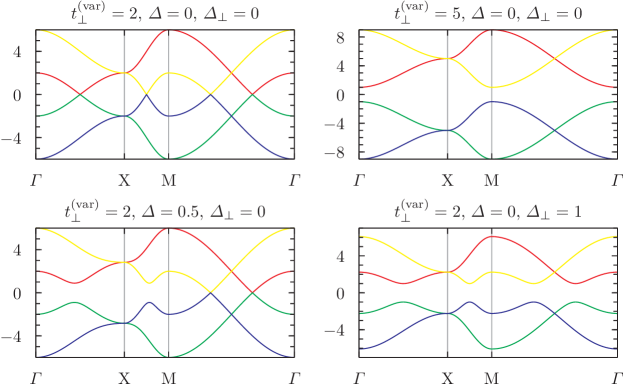
Figure 3: Band structure of the Slater determinant, compare equation (18) and (19), for different values of the variational parameters. The symmetry points are $\Gamma\equiv(0,0)$, $X\equiv(\pi,0)$ and $M\equiv(\pi,\pi)$. The blue and green band are occupied, and a gap opens for $t^{\mathrm{(var)}}_{\perp}>4$ or $\Delta_{\perp}\neq 0$. As expected, the in-plane pairing $\Delta$ does not open a gap in the $d$-wave’s nodal direction $\Gamma\rightarrow M$.

It can easily be seen that there are two ways of opening a gap in the mean field part of our variational wavefunction, namely having a $t^{\mathrm{(var)}}_{\perp}>4$, or a non-zero $\Delta_{\perp}$ which corresponds to the formation of singlets between the planes. We now discuss the variational Monte Carlo simulation results used to draw the non-magnetic phase diagram in figure 2.

Figure 4 shows the optimized interplane pairing $\Delta_{\perp}$ as a function of the interplane hopping $t_{\perp}$.

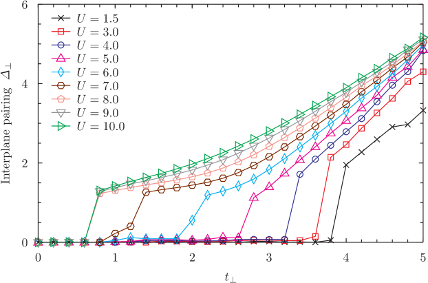
Figure 4: Interplane pairing $\Delta_{\perp}$ as a function of the interplane hopping $t_{\perp}$ for the non-magnetic phase diagram of figure 2. The system becomes a band insulator for $\Delta_{\perp}\neq 0$ (compare with figure 3).

Starting with $t_{\perp}=4$ at $U=0$ the region with a non-zero $\Delta_{\perp}$ extends to lower $t_{\perp}$ as $U$ is increased. For $U\geq 8$ the jump is at a constant $t_{\perp}\approx 0.7$. As any non-zero $\Delta_{\perp}$ opens a gap in the mean field part of the wavefunction, the region of a non-zero $\Delta_{\perp}$ maps out the band insulating part of the phase diagram in figure 2.

At variance with the band insulator, a Mott insulating region is characterized by a gapless mean-field state, while the insulating nature is driven by the electronic correlations that are included in the Jastrow factor $\hat{\mathcal{P}}_{J}$. In order to discriminate between a Mott insulator and a metal, we use the following single mode ansatz for the wavefunction of the excited state, which goes back to Richard Feynman’s work on excitations in liquid Helium [49], and was later successfully applied to fermionic systems: [50][51]

$$\ket{\Psi_{\mathbf{q}}}=\hat{n}_{\mathbf{q}}\ket{\Psi_{0}}\,,$$ (20)

where $\hat{n}_{\mathbf{q}}$ is the Fourier transform of the particle density with $\mathbf{q}=(q_{x},q_{y},0)$. By calculating the energy of the excited state, one can derive a formula for an upper bound of the charge gap $E_{g}$, that relates it to the static structure factor $N(\mathbf{q})=\langle\hat{n}_{-\mathbf{q}}\;\hat{n}_{\mathbf{q}}\rangle$: [52]

$$E_{g}\propto\lim_{\mathbf{q}\rightarrow 0}\frac{|\mathbf{q}|^{2}}{N(\mathbf{q})}\,.$$ (21)

Figure 5 shows the charge gap $E_{g}$ as a function of the Coulomb repulsion $U$ for different interplane hoppings $t_{\perp}$.

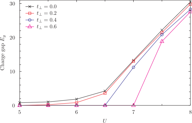
Figure 5: Charge gap $E_{g}$ for the non-magnetic phase diagram (in arbitrary units, compare equation 21) as a function of the Coulomb repulsion $U$.

As expected from the known monolayer results, we find the system to be a Mott insulator for large enough values of $U$. Note that the critical $U$ needed to make the system Mott insulating, i.e. when the charge gap $E_{g}$ starts to grow as a function of $U$, increases from about $U=5.5$ at $t_{\perp}=0$ to $U=7.5$ at $t_{\perp}=0.6$. Note that a finite charge gap for $U\lesssim 5.5$ and $t_{\perp}=0$ is just an artefact of the limited number of $\mathbf{q}$ points that are available for the extrapolation to $\mathbf{q}=0$ and indeed decreases as the system size increases. We point out that a sizeable in-plane $\Delta$ can be found only in the Mott insulating region, indicating that the pairing within the planes is to be understood in terms of the resonating valence bond theory [53, 54], in which $d$-wave pairs are formed, but not phase coherent. Indeed, it is the presence of the Jastrow factor of equation (16), that allows the $\hat{{\mathcal{P}}}_{J}\ket{\Phi}$ wave function to describe a Mott insulator through the opening of a charge gap without any symmetry breaking.

Figure 6 shows the renormalization of the variational interplane hopping $t^{\mathrm{(var)}}_{\perp}$.

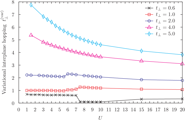
Figure 6: The variational interplane hopping $t^{\mathrm{(var)}}_{\perp}$ as a function of the Coulomb repulsion $U$ for different values of the interplane hopping $t_{\perp}$ in the original Hubbard Hamiltonian. The results are for the non-magnetic phase diagram.

In general the variational $t^{\mathrm{(var)}}_{\perp}$ is not too different from the $t_{\perp}$ in the original Hubbard Hamiltonian, but there are two exceptions to this rule. The first one is that in the Mott insulating phase (at large $U$ and small $t_{\perp}$) the variational $t^{\mathrm{(var)}}_{\perp}$ is renormalized to quite small values. Together with the lack of a $\Delta_{\perp}$ in this region, this indicates that the mean field part of the wavefunction is almost that of two decoupled Hubbard planes. The other exception is that for small $U$ and large $t_{\perp}$ the variational $t^{\mathrm{(var)}}_{\perp}$ is renormalized to values larger than the original $t_{\perp}$. This is due to the fact that in the limit $U\to 0$ the ground-state wavefunction is independent of the value of $t_{\perp}$ with the bonding band filled as long as $t_{\perp}>4$.

The band gap and the Mott gap opening via $\Delta_{\perp}$, presented in figure 4 and figure 5 respectively, suffice for mapping out the regions of band and Mott insulators in the phase diagram. The physics of the respective transitions can be confirmed by looking at the density of double occupancies presented in figure 7, as a function of the interplane hopping $t_{\perp}$.

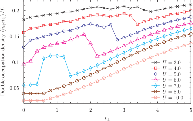
Figure 7: For the non-magnetic phase diagram, figure 2, the density of double occupancies as a function of the interplane hopping $t_{\perp}$.

For intermediate values of $U$, the density of double occupancies first rises sharply and then drops off abruptly again as the $t_{\perp}$ is increased, signalling that there is a metallic phase in between the Mott and band insulating phases for $5.5\lesssim U\lesssim 7.5$. The double occupation density was also calculated within $2\times 2$ cluster DMFT [9], but, contrary to our results of figure 7, it was found that it decreases in the metallic phase. We believe that our results correspond to the physics of the Mott insulating phase, which suppresses double occupancies.

At large $U\gtrsim 8$ the Mott insulator goes directly into the band insulator at $t_{\perp}\approx 0.7$. The Mott insulating wavefunction is characterized by an in-plane $\Delta>0$ and a $\Delta_{\perp}=0$, while the band insulating wavefunction has a sizeable $\Delta_{\perp}$ but no in-plane $\Delta$. A strong hysteresis in these variational parameters was observed when going through the transition, so that both a Mott and a band insulator could be obtained for $t_{\perp}$ close to the transition. The optimal wavefunction is the one with the lowest energy, as plotted in figure 8.

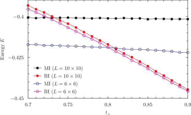
Figure 8: The energy of both Mott and band insulating wavefunctions for different values of $t_{\perp}$ close to the Mott to band insulator transition. Note that increasing the system size from $36$ to $100$ sites per plane slightly decreases the critical $t_{\perp}$ from $0.8$ to $0.73$. The data is for the non-magnetic phase diagram.

Finding hysteresis means that both the Mott and the band insulating wavefunctions are local energy minima in our variational parameter space, thus suggesting that the Mott to band insulator transition is of first order.

3.2 The magnetic phase diagram

The simulations through which the magnetic phase diagram was obtained were performed in the same way as those for the non-magnetic case, except that the site and spin dependent chemical potential $\mu_{m}$ of equation (13) was no longer fixed to zero during the optimization.

Figure 9 shows the magnetic potential $\mu_{m}$, as a function of the interplane hopping $t_{\perp}$.

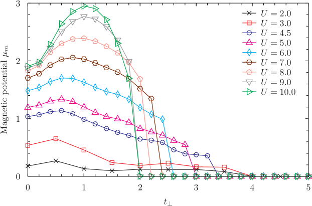
Figure 9: The magnetic potential $\mu_{m}$ as a function of the interplane hopping $t_{\perp}$.

For small $U$ an antiferromagnetic order is found for $t_{\perp}<4$, since the ordering is driven by the perfect nesting of the Fermi surfaces corresponding to partially filled bonding and antibonding bands. The Fermi surface no longer exists if the bonding band is completely filled and the antibonding band completely empty at $t_{\perp}>4$. Increasing $U$ pushes the antiferromagnetic region to smaller $t_{\perp}$, indicating that the critical interplane hopping goes to the Heisenberg limit of $t_{\perp}=1.588$ for $U\rightarrow\infty$.

One can show, by analogy to the non-magnetic case in the previous section, that any non-zero $\mu_{m}$ makes the system insulating by analytically diagonalizing the variational single particle Hamiltonian:

$$\hat{H}_{\mathrm{var}}=\hat{H}_{t}+\hat{H}^{\mathrm{(var)}}_{t_{\perp}}+\hat{H}_{\mathrm{mag}}\,,$$ (22)

which leads to the results

$$\epsilon^{(1,3)}_{\mathbf{k}} =\pm\sqrt{\big{(}-2t(\cos k_{x}+\cos k_{y})+t_{\perp}\big{)}^{2}+\mu_{m}^{2}}$$ (23)

$$\epsilon^{(2,4)}_{\mathbf{k}} =\pm\sqrt{\big{(}-2t(\cos k_{x}+\cos k_{y})-t_{\perp}\big{)}^{2}+\mu_{m}^{2}}\,.$$ (24)

The two negative bands are filled and the system can only be conducting if these bands touch the empty bands at zero energy. Looking at the equations for the energy bands, one can see that this can not happen for $\mu_{m}\neq 0$, and hence one can use a non-zero $\mu_{m}$ as a criterion for an insulating state. Note that we classify the ordered state in the phase diagram (figure 2, right panel) as a Mott insulator, even though we have a gap in the mean field state. This is due to the fact that the antiferromagnetic ordering is correlation induced.

Comparing the interplane $\Delta_{\perp}$ in figure 10

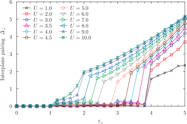
Figure 10: The interplane pairing $\Delta_{\perp}$ as a function of the interplane hopping $t_{\perp}$ for the magnetic phase diagram of figure 2.

with the plot of the magnetic potential $\mu_{m}$ in figure 9, we see that a non-zero $\Delta_{\perp}$ is found in the entire paramagnetic region. Both the $\mu_{m}$ and the $\Delta_{\perp}$ open a gap in the mean field part of the wavefunction, so that the square lattice bilayer Hubbard model is always an insulator at $U>0$ if magnetic order is allowed.

It is interesting to note that at large $U\gtrsim 8$ and $1<t_{\perp}\lesssim 2$ there is a small region with both a non-zero magnetic potential $\mu_{m}$ and an interplane pairing $\Delta_{\perp}$. This, together with the fact that no hysteresis in the variational parameters was observed at the order-disorder transition, suggests that the transition is indeed continuous.

4 Conclusion

In summary we have calculated the magnetic and non-magnetic phase diagram of the square lattice bilayer Hubbard model using the variational Monte Carlo method, as summarized in figure 2. Moreover, our results suggest that the Mott insulator to band-insulator transition is of first order in the non-magnetic phase diagram, while it becomes continuous when magnetic order is allowed.

Comparison of our results to the ones obtained with DMFT [8] and cluster DMFT [9] reveals that our non-magnetic phase diagram includes some features observed in DMFT and $2\times 2$ cluster DMFT but also new distinct properties: While in agreement with $2\times 2$ cluster DMFT there is a region in which the system first goes from a Mott insulator to a metal and then to a band insulator as $t_{\perp}$ is increased, we do not find that this region extends down to $U=0$. Instead for the decoupled planes we find a metal to Mott insulator transition at a critical $U\approx 5.5$, which agrees with the DMFT results by Fuhrmann et al, and the dynamical cluster approximation results for the single layer by Gull et al [29]. For large $U$ our results agree with those of $2\times 2$ cluster DMFT in that there is a direct transition from a Mott to a band insulator, but our critical $t_{\perp}$ is smaller by about a factor of 3. The reason for this might be the cluster with two sites in each plane used by the authors of reference [9] that breaks the fourfold rotational symmetry of the square lattice and creates an artificially enhanced local pair within each plane, ultimately stabilizing the in-plane Mott phase against the interplane dimers of the band insulating phase.

The magnetic phase diagram, instead, shows clearly a different behaviour from the one predicted by $2\times 2$ cluster DMFT calculations. The most obvious difference is that we no longer find a metallic phase if magnetic ordering is allowed. Instead we find a Néel ordered Mott insulator, which we attribute to the perfect nesting between the bonding and antibonding band’s Fermi surfaces. The reason for the variational Monte Carlo approach stabilizing magnetic ordering compared to cluster DMFT with two sites per plane might be the much more explicit treatment of long range correlations.

The variational Monte Carlo results improve our understanding of the bilayer Hubbard model, but further investigation may be necessary to clarify the origin of the sizeable differences between VMC and DMFT results.

References

References

- [1] Satoshi Ejima and Satoshi Nishimoto. Phase Diagram of the One-Dimensional Half-Filled Extended Hubbard Model. Phys. Rev. Lett., 99:216403, 2007.
- [2] C. D. Batista and A. A. Aligia. Exact Bond Ordered Ground State for the Transition between the Band and the Mott Insulator. Phys. Rev. Lett., 92:246405, 2004.
- [3] Arti Garg, H. R. Krishnamurthy, and Mohit Randeria. Can Correlations Drive a Band Insulator Metallic? Phys. Rev. Lett., 97:046403, 2006.
- [4] S. S. Kancharla and E. Dagotto. Correlated Insulated Phase Suggests Bond Order between Band and Mott Insulators in Two Dimensions. Phys. Rev. Lett., 98:016402, 2007.
- [5] K. Bouadim, N. Paris, F. Hébert, G. G. Batrouni, and R. T. Scalettar. Metallic phase in the two-dimensional ionic Hubbard model. Phys. Rev. B, 76:085112, 2007.
- [6] Hui-Min Chen, Hui Zhao, Hai-Qing Lin, and Chang-Qin Wu. Bond-located spin density wave phase in the two-dimensional (2d) ionic Hubbard model. New Journal of Physics, 12(9):093021, 2010.
- [7] Michael Sentef, Jan Kuneš, Philipp Werner, and Arno P. Kampf. Correlations in a band insulator. Phys. Rev. B, 80:155116, 2009.
- [8] Andreas Fuhrmann, David Heilmann, and Hartmut Monien. From Mott insulator to band insulator: A dynamical mean-field theory study. Phys. Rev. B, 73:245118, 2006.
- [9] S. S. Kancharla and S. Okamoto. Band insulator to Mott insulator transition in a bilayer Hubbard model. Phys. Rev. B, 75:193103, 2007.
- [10] K. Bouadim, G. G. Batrouni, F. Hébert, and R. T. Scalettar. Magnetic and transport properties of a coupled Hubbard bilayer with electron and hole doping. Phys. Rev. B, 77:144527, 2008.
- [11] H. Hafermann, M. I. Katsnelson, and A. I. Lichtenstein. Metal-insulator transition by suppression of spin fluctuations. EPL, 85(3):37006, 2009.
- [12] B.D. Napitu and J. Berakdar. Traces of the evolution from Mott insulator to a band insulator in the pair excitation spectra. Eur. Phys. J. C, 85(2):1–10, 2012.
- [13] A. Euverte, S. Chiesa, R. T. Scalettar, and G. G. Batrouni. Magnetic transition in a correlated band insulator. Phys. Rev. B, 87:125141, 2013.
- [14] Louk Rademaker, Steve Johnston, Jan Zaanen, and Jeroen van den Brink. Determinant quantum Monte Carlo study of exciton condensation in the bilayer Hubbard model. Phys. Rev. B, 88:235115, 2013.
- [15] Hunpyo Lee, Yu-Zhong Zhang, Harald O. Jeschke, and Roser Valentí. Competition between band and mott insulators in the bilayer hubbard model: A dynamical cluster approximation study. Phys. Rev. B, 89:035139, Jan 2014.
- [16] Andrea Damascelli, Zahid Hussain, and Zhi-Xun Shen. Angle-resolved photoemission studies of the cuprate superconductors. Rev. Mod. Phys., 75:473–541, 2003.
- [17] D. Fournier et al. Loss of nodal quasiparticle integrity in underdoped YBa2Cu3O6+x. Nat. Phys., 6:905–911, 2010.
- [18] Antoine Georges, Gabriel Kotliar, Werner Krauth, and Marcelo J. Rozenberg. Dynamical mean-field theory of strongly correlated fermion systems and the limit of infinite dimensions. Rev. Mod. Phys., 68:13–125, 1996.
- [19] M. H. Hettler, A. N. Tahvildar-Zadeh, M. Jarrell, T. Pruschke, and H. R. Krishnamurthy. Nonlocal dynamical correlations of strongly interacting electron systems. Phys. Rev. B, 58:R7475–R7479, 1998.
- [20] M. Jarrell, Th. Maier, C. Huscroft, and S. Moukouri. Quantum Monte Carlo algorithm for nonlocal corrections to the dynamical mean-field approximation. Phys. Rev. B, 64:195130, 2001.
- [21] A. I. Lichtenstein and M. I. Katsnelson. Antiferromagnetism and -wave superconductivity in cuprates: A cluster dynamical mean-field theory. Phys. Rev. B, 62:R9283–R9286, 2000.
- [22] Thomas Maier, Mark Jarrell, Thomas Pruschke, and Matthias H. Hettler. Quantum cluster theories. Rev. Mod. Phys., 77:1027–1080, 2005.
- [23] Gabriel Kotliar, Sergej Y. Savrasov, Gunnar Pálsson, and Giulio Biroli. Cellular Dynamical Mean Field Approach to Strongly Correlated Systems. Phys. Rev. Lett., 87:186401, 2001.
- [24] J. E. Hirsch. Two-dimensional Hubbard model: Numerical simulation study. Phys. Rev. B, 31:4403–4419, 1985.
- [25] N. D. Mermin and H. Wagner. Absence of Ferromagnetism or Antiferromagnetism in One- or Two-Dimensional Isotropic Heisenberg Models. Phys. Rev. Lett., 17:1133–1136, 1966.
- [26] Claudius Gros, Wolfgang Wenzel, and Johannes Richter. The transition from an ordered antiferromagnet to a quantum disordered spin liquid in a solvable bilayer model. Europhys. Lett., 32(9):747, 1995.
- [27] A. W. Sandvik and D. J. Scalapino. Order-disorder transition in a two-layer quantum antiferromagnet. Phys. Rev. Lett., 72:2777–2780, 1994.
- [28] Ling Wang, K. S. D. Beach, and Anders W. Sandvik. High-precision finite-size scaling analysis of the quantum-critical point of Heisenberg antiferromagnetic bilayers. Phys. Rev. B, 73:014431, 2006.
- [29] Emanuel Gull, Olivier Parcollet, and Andrew J. Millis. Superconductivity and the Pseudogap in the Two-Dimensional Hubbard Model. Phys. Rev. Lett., 110:216405, 2013.
- [30] Luca F. Tocchio, Federico Becca, and Claudius Gros. Strong renormalization of the Fermi-surface topology close to the Mott transition. Phys. Rev. B, 86(3):035102, 2012.
- [31] Manuela Capello, Federico Becca, Seiji Yunoki, and Sandro Sorella. Unconventional metal-insulator transition in two dimensions. Phys. Rev. B, 73:245116, 2006.
- [32] Hunpyo Lee, Yu-Zhong Zhang, Harald O. Jeschke, Roser Valentí, and Hartmut Monien. Dynamical Cluster Approximation Study of the Anisotropic Two-Orbital Hubbard Model. Phys. Rev. Lett., 104:026402, 2010.
- [33] W. L. McMillan. Ground State of Liquid . Phys. Rev., 138:A442–A451, 1965.
- [34] D. Ceperley, G. V. Chester, and M. H. Kalos. Monte Carlo simulation of a many-fermion study. Phys. Rev. B, 16:3081–3099, 1977.
- [35] Walter Ritz. Über eine neue Methode zur Lösung gewisser Variationsprobleme der mathematischen Physik. J. Reine Angew. Math., 135:1–61, 1909.
- [36] Robert Rüger. Implementation of the Variational Monte Carlo method for the Hubbard model. Master’s thesis, Goethe University Frankfurt, 2013.
- [37] Claudius Gros. Physics of projected wavefunctions. Annals of Physics, 189(1):53–88, 1989.
- [38] Roser Valentí and Claudius Gros. Luttinger liquid instability of the 2d model: A variational study. Phys. Rev. Lett., 68(15):2402, 1992.
- [39] Bernhard Edegger, V. N. Muthukumar, and C. Gros. Gutzwiller–RVB theory of high-temperature superconductivity: Results from renormalized mean-field theory and variational Monte Carlo calculations. Adv. Phys., 56(6):927–1033, 2007.
- [40] Claudius Gros. Superconductivity in correlated wave functions. Phys. Rev. B, 38:931–934, 1988.
- [41] F. C. Zhang, C. Gros, T. M. Rice, and H. Shiba. A renormalised Hamiltonian approach to a resonant valence bond wavefunction. Superconductor Science and Technology, 1(1):36, 1988.
- [42] Nejat Bulut, Douglas J. Scalapino, and Richard T. Scalettar. Nodeless -wave pairing in a two-layer Hubbard model. Phys. Rev. B, 45:5577–5584, 1992.
- [43] Luca F. Tocchio, Federico Becca, Alberto Parola, and Sandro Sorella. Role of backflow correlations for the nonmagnetic phase of the Hubbard model. Phys. Rev. B, 78:041101, 2008.
- [44] Federico Becca, Massimo Capone, and Sandro Sorella. Spatially homogeneous ground state of the two-dimensional Hubbard model. Phys. Rev. B, 62:12700–12706, 2000.
- [45] Manuela Capello, Federico Becca, Michele Fabrizio, Sandro Sorella, and Erio Tosatti. Variational Description of Mott Insulators. Phys. Rev. Lett., 94:026406, 2005.
- [46] Nicholas Metropolis, Arianna W. Rosenbluth, Marshall N. Rosenbluth, Augusta H. Teller, and Edward Teller. Equation of State Calculations by Fast Computing Machines. J. Chem. Phys., 21(6):1087–1092, 1953.
- [47] Sandro Sorella. Generalized Lanczos algorithm for variational quantum Monte Carlo. Phys. Rev. B, 64:024512, 2001.
- [48] Michele Casula, Claudio Attaccalite, and Sandro Sorella. Correlated geminal wave function for molecules: An efficient resonating valence bond approach. J. Chem. Phys., 121(15):7110–7126, 2004.
- [49] R. P. Feynman. Atomic Theory of the Two-Fluid Model of Liquid Helium. Phys. Rev., 94:262–277, 1954.
- [50] A. W. Overhauser. Simplified Theory of Electron Correlations in Metals. Phys. Rev. B, 3:1888–1898, 1971.
- [51] S. M. Girvin, A. H. MacDonald, and P. M. Platzman. Magneto-roton theory of collective excitations in the fractional quantum Hall effect. Phys. Rev. B, 33:2481–2494, 1986.
- [52] Luca F. Tocchio, Federico Becca, and Claudius Gros. Backflow correlations in the Hubbard model: An efficient tool for the study of the metal-insulator transition and the large- limit. Phys. Rev. B, 83:195138, 2011.
- [53] P. W. Anderson. The Resonating Valence Bond State in La2CuO4 and Superconductivity. Science, 235(4793):1196–1198, 1987.
- [54] Claudius Gros, D. Poilblanc, T. M. Rice, and F. C. Zhang. Superconductivity in correlated wavefunctions. Phys. C Supercond., 153:543–548, 1988.