Evaluating the Impact of SDC on the GMRES Iterative Solver

Abstract

Increasing parallelism and transistor density, along with increasingly tighter energy and peak power constraints, may force exposure of occasionally incorrect computation or storage to application codes. Silent data corruption (SDC) will likely be infrequent, yet one SDC suffices to make numerical algorithms like iterative linear solvers cease progress towards the correct answer. Thus, we focus on resilience of the iterative linear solver GMRES to a single transient SDC. We derive inexpensive checks to detect the effects of an SDC in GMRES that work for a more general SDC model than presuming a bit flip. Our experiments show that when GMRES is used as the inner solver of an inner-outer iteration, it can “run through” SDC of almost any magnitude in the computationally intensive orthogonalization phase. That is, it gets the right answer using faulty data without any required roll back. Those SDCs which it cannot run through, get caught by our detection scheme.

I Introduction

Incorrect arithmetic or corruption of stored data could have dire effects on the execution of a numerical algorithm. Experiments show that a single bit flip in memory can cause certain algorithms to “crash” (terminate abnormally, due to invalid states or actions detected by the application or operating system), “stagnate” (keep running but fail to make progress), or, worst of all, produce the wrong solution, silently.

Rather than focusing exclusively on bit flips, this work studies the impact of Silent Data Corruption (SDC) on the Generalized Minimal Residual Method (GMRES) iterative linear solver. The source of the corruption, while interesting, gives no insight into its impact on the algorithm and the correctness of its result. By generalizing bit flips in floating-point data into potentially unbounded numerical errors, we are able to use mathematical analysis both to reason about algorithms’ behavior should an SDC event occur, and to harden them against the event’s effects.

Fortunately, some numerical algorithms only need reliability for certain data and phases of computation. If the system can guard just those parts of the algorithm in space and time, then the algorithm can compute the right answer — or at least be able to detect failure and report it “loudly” — despite faults in unreliable phases of execution. This suggests a “layered” approach to the design of reliable numerical algorithms. A reliable outer layer can recover from faults in a less reliable inner layer. If the solver spends most of its time in unreliable mode, it can mitigate the cost of reliable computation in the outer mode. We begin the analysis with GMRES, and then extend it to the Fault-Tolerant GMRES (FT-GMRES) inner-outer iteration.

We present the following contributions:

• We use mathematical analysis of the GMRES algorithm to construct a detector that bounds the error that SDC may introduce.

• We combine the above detection scheme with the sandbox reliability model presented in [1].

• We illustrate experimentally that bounded error originating in the faulty inner solve has little impact on time-to-solution.

I-A Silent Data Corruption

In this work, we address a very specific type of fault, i.e., a fault that silently introduces bad data, while not persistently tainting the data that was used in the calculation. For example, let $a=2$ and $b=2$, then $c=a+b=10$, while simplistic, this model presumes no knowledge of the nature of the fault, only that $c$ is incorrect. This model assumes that the machine is unreliable in an unpredictable way, and therefore we are skeptical of the output it presents. This type of unreliability can be mitigated via redundant computation and introspection, but then the cost of running the algorithm increases drastically.

I-B Faults, Failures, and Persistence

Our goal is to ensure that should transient SDC occur, we either obtain the correct solution or make the fault not silent by alerting the user. We consider two perspectives: the user and the system. A fault occurs at the system level, e.g., a bit flips or a node crashes. A fault becomes a failure if it impacts the user. Figure 1 depicts a visual taxonomy of how we consider faults and the scope of our work. We further classify faults into those that interrupt the user’s program (hard faults), and those that do not immediately or ever interrupt the user’s code (soft faults). A hard fault results in a failure if the user is running an application (though a checkpoint / restart recovery system can “mask out” hard faults, making them not failures). In contrast, the very nature of soft faults implies that they may emit no indication that something has gone wrong. In the event that soft faults allow the program to continue execution with tainted data, we must understand how algorithms behave in the presence of faulty data. Furthermore, if the algorithm uses tainted data and still obtains the correct solution, then the fault does not constitute a failure. If the soft fault leads to an incorrect solution, then the fault leads to a silent failure, which is an outcome we wish to make very rare or impossible.

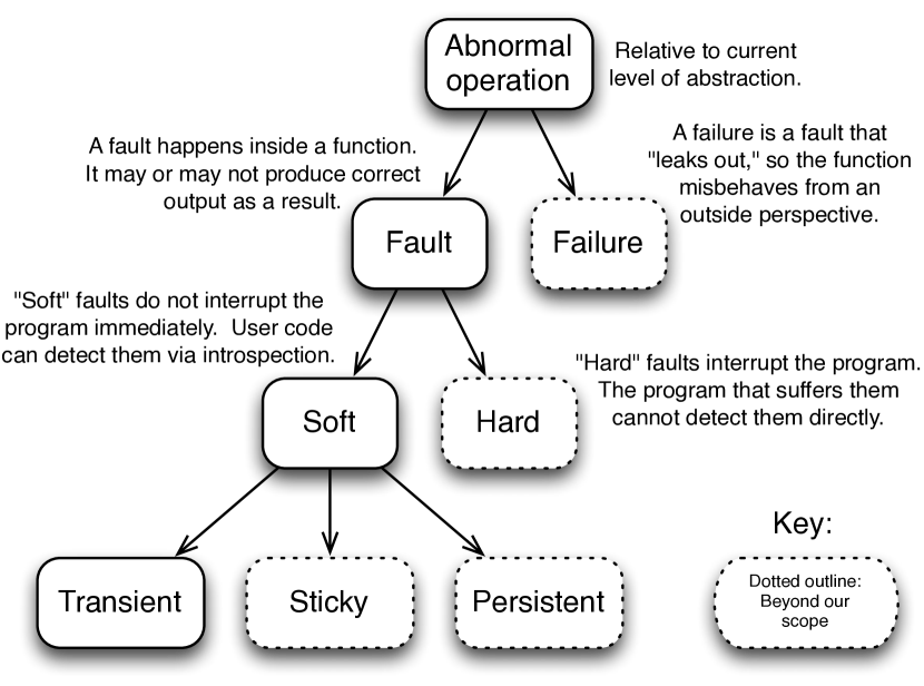
Figure 1: Taxonomy of faults and scope of this work.

We further classify soft faults by how long the underlying hardware remains faulty. Persistent faults arise from hardware that is permanently faulty, e.g., a stuck bit in memory, or the Intel Pentium FDIV bug [2]. Sticky faults indicate hardware that is faulty for some duration but returns to normal operation. Transient faults occur once, and while the fault is transient the effect of the fault may be persistent.

II Project Overview

To quantify the possible effects of a single silent data corruption event in GMRES, we propose a multifaceted approach. We combine the sandbox reliability model from [1], Flexible GMRES from Saad [3], and mathematical analysis of the GMRES algorithm to create a nested solver strategy that combines an unreliable inner solver with a reliable outer solver, while enforcing that, should SDC occur in the unreliable phase, the error is bounded. We then show through experiments how our scheme “runs through” single SDC events in the unreliable solver. Using this approach, we ultimately seek to present analyses of solvers such that we can quantitatively choose solvers based on their resiliency to single events of SDC.

This paper is organized as follows:

1. In Section IV, we describe the sandbox reliability model.

2. In Section V, we present standard GMRES, and uncover through mathematical analysis an invariant in the Arnoldi process contained within GMRES.

3. We describe how to check this invariant when using Modified Gram-Schmidt orthogonalization.

4. In Section VI, we introduce Saad’s Flexible GMRES and Bridges et al.’s FT-GMRES, and explain the relation between flexible solvers and the sandbox reliability model.

5. In Section VII, we compose a nested solver using the Trilinos framework [4], and present experimental results illustrating how our invariant check impacts time-to-solution.

II-A Assumptions and Justification

We restrict SDC to the numerical data used and generated by the algorithm. We explicitly exclude faults in control flow, data structures, loop counters and other metadata used to implement the algorithm. The reason for this exclusion is that these issues represent a different class of problems.

Our assumption that SDC occurs only once is fundamental. The implied source of SDC is typically a bit flip, but we do not restrict our model to silent bit upsets, given that there is limited data available today to base such a model on. We justify our choice of single transient SDC, based on what we do know about bit flips and the reliability of the system:

1. Hardware employs techniques to ensure that so-called “single event upsets” (SEUs) – that is, bit flips – do not occur. Therefore, it is expected that SEUs will be rare events.

2. If we can understand the best- and worst-case scenarios for the error that an SDC can contribute, we will have a baseline to conjecture about multiple bit flips, i.e., multiple occurrences of SDC.

3. There currently is no solid theory, e.g., a statistical distribution, of the rate at which bit flips occur. Therefore, speculation about flip rates may or may not prove useful.

4. Assuming a particular fault rate makes bold assertions about future hardware, especially given the reluctance of hardware manufacturers to divulge this information.

By following this research path, we are able to avoid the pitfalls presented in items 3 and 4 above, and we are able to isolate the impact of SDC without other factors polluting our analysis.

III Motivation

Energy and peak power increasingly constrain modern computer hardware, yet hardware approaches to protect computations and data against errors cost energy. This holds at all scales of computation, but especially for the largest parallel computers being built and planned today. This results from a confluence of factors:

• Increasing parallelism (and therefore more components to fail) [5, 6]

• Decreasing transistor feature sizes, making individual components more vulnerable

• Extremely tight peak power requirements [7], limiting the use of hardware redundancy to increase reliability

As these trends continue, hardware vendors may succumb to the temptation to expose incorrect arithmetic or memory corruption to application codes [8, 7, 9]. Some studies already indicate that this behavior is appearing at the user level [10]. In fact, some researchers actively promote relaxing hardware correctness to save energy [11].

III-A Relation to Prior Work

Much of the prior work on fault-tolerant iterative solvers has taken the approach of assuming some fault model for bit flips, and then injecting bit flips into specific numerical operations [12, 13, 14], or treating the application as a black box and injecting bit flips arbitrarily [15]. A popular operation to analyze is sparse matrix-vector multiply [12, 14], a key kernel in iterative linear solvers. These approaches typically engineer a response that mitigates, detects, or detects and corrects bit flips injected following the assumed fault model. The focus in this type of research has been to detect errors, and then respond – e.g., correct the tainted values, or roll back and resume computation from an assumed valid state – assuming that the fault does not occur frequently enough to cause stagnation.

In addition, all prior work on sparse iterative methods is based on a fault model that assumes multiple bit flips injected at some rate. Most studies are also carried out with little care for whether the bit flipped is a $0\to 1$ or a $1\to 0$, and most studies flip bits at random locations. We question many of the assumptions made, and in general question the research approach.

III-A1 SDC is a rare event

We begin by questioning models and experiments that assume SDC happens at a sufficiently high rate for multiple events to occur in a single linear solve.

We have a strong reason to believe that SDC is a rare event. Hardware incorporates a fairly large amount of safeguards in-place to protect data and instructions. For example, Intel provides the Machine Check Architecture, which provides reporting of bit errors at the register, cache (L1-L3), QuickPath Interconnect, and DRAM (via ECC) layers. We do not attempt to conjecture about the likelihood of bit flips, rather we turn to the theoretical basis that an algorithm is built on, and study how the algorithm behaves when perturbed within the bounds imposed by mathematical analysis.

Current research by Michalak [16] found SDC occurred rarely. Michalak et al. placed a Roadrunner node in front of a neutron cannon and bombarded it with particles [16]. While the neutron fluxes are far beyond realistic, their observations showed a startlingly low occurrence of SDC, while outright node failure occurred far more frequently. Why then has current SDC research focused on failure rates?

In practice, SDCs should remain rare, even at extreme scales of parallelism. Nevertheless, little if any current research has attempted to explain how a single SDC event impacts an algorithm and ultimately the solution. Research on how to counter multiple bit flips has not provided additional insight on the cause/effect relationship.

Also, an application may attribute much of its run time to linear solves, but typically these are multiple linear solves, e.g., an implicit time stepping algorithm that solves a nonlinear system at each time step. For example, see Müller and Scheichl where a nonlinear system of size $10^{10}$ is solved and the linear solver is restricted to $0.003$ seconds per solve [17].

III-A2 Fault Models and Silent Data Corruption

At a higher level, we challenge the research approach of assuming a fault model for SDC. By definition, the origin of silent data corruption is unknown, with one such origin being a silent bit flip. Instead of characterizing SDC, the studies propose solutions to a problem we understand only poorly. It is our goal first to analyze the effects of SDC, and then to propose both specific algorithmic techniques and general heuristics that minimize its impact, should it occur. With this ability, mathematicians, scientists, and engineers can take quantifiable steps to develop algorithms and applications that are inherently resilient to SDC.

In numerical algorithms using IEEE-754 floating-point data, regardless of the cause, SDC will produce either numeric values or the non-numeric infinity (Inf) and not-a-number (NaN) values. Injecting bit flips will produce either type of error, making the act of injecting a bit flip to study transient SDC unnecessary as the outcome could have been achieved by merely setting the memory location equal to some value. We know from the IEEE-754 specification precisely what numeric values are possible, and given the mystery of how, when, and where SDC originates, any of the possible floating-point values are plausible.

We advocate a drastically different approach, namely that SDC impacts the underlying mathematical assumptions that guarantee convergence of an algorithm. Rather than focusing on detecting binary errors, we treat bit flips as numerical errors and evaluate how these errors relate to the theoretical basis that the algorithm is built on. In this sense, we filter values that are theoretically impossible, while accepting variations that are allowable by the theory. While our approach does not “solve” the SDC problem, we exploit modern mathematical techniques, so-called flexible solves, to cope with the bounded error we “run through”.

III-B Invariants as Detectors

Numerical algorithms often have invariants that they can check inexpensively to decide whether hardware faults have corrupted an intermediate result enough for it not to be useful. For example, Chen [18] performs additional computation and parallel communication in order to check invariants of the iterative linear solvers GMRES [19], CG, and BiCG. If those invariants are violated, the solver can roll back one or more iterations and resume from the last known correct point. In this work, we develop invariants that require no additional parallel communication and very little extra computation to check. This reduces the amount of state needed to roll back correctly, since we can afford to check these invariants at every iteration. In fact, GMRES (and variants, like “Flexible GMRES”) keeps enough state on its own that, unlike in Chen’s work, we do not need to save anything to a persistent store.

Checking invariants naturally fits into the layered approach we mentioned in the introduction. In the case of FT-GMRES, the outer solver (based on Flexible GMRES [3]) can check the results of the unreliable inner solves by computing a residual reliably. The outer solver will never compute the wrong answer, no matter what the inner solves do. We present findings in this paper that indicated that a layered approach coupled with our theory-based detector can tolerate a single SDC event with little (if any) impact on convergence.

IV Sandbox Reliability

Relaxing reliability of all data and computations may result in all manner of undesirable and unpredictable behavior. If instructions, pointers, array indices, and Boolean values used for decisions may change arbitrarily at any time, we cannot assert anything about the results of a computation or the side effects of the program, even if it runs to completion without abnormal termination. The least we can do is force the fault-susceptible program to execute in a sandbox. This is a general idea from computer security, that allows the execution of untrusted “guest” code in a partition of the computer’s state (the “sandbox”) that protects the rest of the computer (the “host”) from the guest’s possibly bad behavior. Sandboxing can even protect the host against malicious code that aims to corrupt the system’s state, so it can certainly handle code subject to unintentional faults in data and instructions.

Sandboxes ensure isolation of a possibly unreliable phase of execution. They allow data to flow between reliable and unreliable phases of execution. Also, they let the host force guest code to stop within a predefined finite time, or if the host suspects the guest may have wandered astray. This feature is especially important in distributed-memory computation for preventing deadlock and other failures due to “crashed” or unresponsive nodes. In general, sandboxing converts some kinds of hard faults into soft faults, and limits the scope of soft faults to the guest subprogram.

Sandboxing may be implemented in different ways. For example, the guest may run in a virtual machine on the same hardware as the host, or the host may be implemented as redundant processes or systems. Guests may run on a fast but unreliable subsystem, and the controlling host program may run on a reliable but slower subsystem. We do not specify or depend on a particular implementation of sandboxing in this paper.

The fault-tolerant inner-outer iteration, described in Section VI, uses the sandbox model. There, the guest program performs the task “Solve a given linear system.” The host program invokes the guest repeatedly for different right-hand sides, and the host performs its own calculations reliably. Finer-grained models of reliability may improve the accuracy of the inner solves, which is what our detector in Section V-B accomplishes.

The sandbox model of reliability makes only two promises of the unreliable guest: it returns something (which may not be correct), and it completes in fixed time. These already suffice to construct a working fault-tolerant iterative method, as we will show in Section VI. However, detecting faults or being able to limit how faults may occur would also be useful. These finer-grained models of reliability can be used to improve accuracy of the iterative method, or to prove more specific promises about its convergence.

V GMRES

The Generalized Minimum Residual method (GMRES) of Saad and Schultz [19] is a Krylov subspace method for solving large, sparse, possibly non-symmetric linear systems of the form $\boldsymbol{\mathbf{A}}\boldsymbol{\mathbf{x}}=\boldsymbol{\mathbf{b}}$. GMRES is based on the Arnoldi process [20], which can also be used to approximate a matrix’s eigenvalues and eigenvectors. GMRES has the convenient property that the residual norm of the approximate solution at each iteration is monotonically non-increasing, assuming correct arithmetic and storage. Its use of orthogonal projections and normalized (to length one) basis vectors also has advantages, that we will discuss below.

We begin this section by explaining how to use properties of the Arnoldi process to detect faults in an iteration of GMRES. We then apply the SDC models we developed above to show how to scale the linear system in a way that enhances fault detection and bounds the possible error of the major computational kernels. We will show in future work that these bounds by themselves do not suffice to bound the solution error. Nevertheless, they can, if one makes inexpensive changes to how GMRES computes the solution update coefficients.

V-A Fault detection via projection coefficients

The norms and inner products that occur in each iteration of the Arnoldi process in GMRES have a bounded absolute value. The bound depends on the norm of the preconditioned matrix, which is inexpensive to estimate. We use this bound to detect faults in all the major computational kernels in GMRES.

Algorithm 1 GMRES

1:Linear system $\boldsymbol{\mathbf{A}}\boldsymbol{\mathbf{x}}=\boldsymbol{\mathbf{b}}$ and initial guess $\boldsymbol{\mathbf{x}}_{0}$

2:Approximate solution $\boldsymbol{\mathbf{x}}_{m}$ for some $m\geq 0$

3:

4:$\boldsymbol{\mathbf{r}}_{0}:=\boldsymbol{\mathbf{b}}-\boldsymbol{\mathbf{A}}\boldsymbol{\mathbf{x}}_{0}$$\triangleright$ Unpreconditioned initial residual vector

5:

6:$\beta:=\left\|\boldsymbol{\mathbf{r}}_{0}\right\|_{2}$, $\boldsymbol{\mathbf{q}}_{1}:=\boldsymbol{\mathbf{r}}_{0}/\beta$

7:

8:for $j=1,2,\dots$ until convergence do

9:

10:$\boldsymbol{\mathbf{v}}_{j+1}:=\boldsymbol{\mathbf{A}}\boldsymbol{\mathbf{q}}_{j}$$\triangleright$ Apply the matrix $A$

11:

12:for $i=1,2,\dots,j$ do$\triangleright$ Orthogonalize

13:

14:$h_{i,j}:=\boldsymbol{\mathbf{q}}_{i}\cdot\boldsymbol{\mathbf{v}}_{j+1}$

15:

16:$\boldsymbol{\mathbf{v}}_{j+1}:=\boldsymbol{\mathbf{v}}_{j+1}-h_{i,j}\boldsymbol{\mathbf{q}}_{i}$

17:end for

18:

19:$h_{j+1,j}:=\left\|\boldsymbol{\mathbf{v}}_{j+1}\right\|_{2}$

20:

21:if $h_{j+1,j}\approx 0$ then

22:

23:Solution is $\boldsymbol{\mathbf{x}}_{j-1}$$\triangleright$ Happy breakdown

24:

25:return

26:end if

27:

28:$\boldsymbol{\mathbf{q}}_{j+1}:=\boldsymbol{\mathbf{v}}_{j+1}/h_{j+1,j}$$\triangleright$ New basis vector

29:

30:$\boldsymbol{\mathbf{y}}_{j}:=\displaystyle\operatornamewithlimits{arg\,min}_{y}\left\|\boldsymbol{\mathbf{H}}({1}\nobreak\mskip 1.0mu\mathpunct{}\nonscript\mkern-3.0mu{:}\mskip 1.0mu{}{j+1},{1}\nobreak\mskip 1.0mu\mathpunct{}\nonscript\mkern-3.0mu{:}\mskip 1.0mu{}{j})\boldsymbol{\mathbf{y}}-\beta\boldsymbol{\mathbf{e}}_{1}\right\|_{2}$

31:

32:$\boldsymbol{\mathbf{x}}_{j}:=\boldsymbol{\mathbf{x}}_{0}+[\boldsymbol{\mathbf{q}}_{1},\boldsymbol{\mathbf{q}}_{2},\dots,\boldsymbol{\mathbf{q}}_{j}]\boldsymbol{\mathbf{y}}_{j}$$\triangleright$ Compute solution update

33:end for

V-B Bounds on the Arnoldi Process

We start our analysis by bounding the dot product which determines the $i$-th upper Hessenberg entry, $h_{i,j}$ of the $j$-th Arnoldi iteration. The Arnoldi process is expressed on Lines 8–28 in Algorithm 1. At its core is an orthogonalization kernel, which we have chosen to be the Modified Gram-Schmidt (MGS) process. Classical Gram-Schmidt or Householder transformations may also be used. As we will demonstrate, our bound is invariant of the orthogonalization algorithm chosen.

The MGS process begins on Line 12 and completes on Line 17. To bound $h_{i,j}$ on Line 14, we exploit a property of orthogonal projections. It is well known that linear transforms utilizing orthogonal matrices are isometric. That is, they preserve the length of the vectors. In $\mathbb{R}^{n}$, the dot product of a vector with a unit-length vector is bounded by the length of the first vector. This means that each $h_{i,j}$ entry is bounded by the length of the vector that starts the orthogonalization process (the vector we wish to make orthogonal). To clarify what “starts” the orthogonalization process means, we step back from an algorithmic formulation, and instead write the orthogonalization kernel as a mathematical expression. For clarity, we will use the Classical Gram-Schmidt expression:

$$\boldsymbol{\mathbf{w}}=\left[\boldsymbol{\mathbf{I}}-\boldsymbol{\mathbf{Q}}^{\text{T}}\boldsymbol{\mathbf{Q}}\right]\boldsymbol{\mathbf{u}}$$ (1)

In Eq (1), the vector $\boldsymbol{\mathbf{u}}$ is what “starts” the orthogonalization process, and $\boldsymbol{\mathbf{w}}$ is the resulting vector, which is orthogonal to all vectors in $\boldsymbol{\mathbf{Q}}$, where $\boldsymbol{\mathbf{Q}}=\{\boldsymbol{\mathbf{q}}_{1},\dotsc,\boldsymbol{\mathbf{q}}_{j}\}$.

Returning to Algorithm 1, what “starts” the orthogonalization process is the vector resulting from Line 10. If we can bound the length of this vector, then we know the maximum absolute value that $h_{i,j}$ can take. Since we want to bound the length of the resulting vector, we take the induced $\ell^{2}$ norm, $\left\|\boldsymbol{\mathbf{v}}_{j+1}\right\|_{2}=\left\|\boldsymbol{\mathbf{A}}\boldsymbol{\mathbf{q}}_{j}\right\|_{2}$,

$$\left\|\boldsymbol{\mathbf{v}}_{j+1}\right\|_{2}\leq\left\|\boldsymbol{\mathbf{A}}\right\|_{2}\left\|\boldsymbol{\mathbf{q}}_{j}\right\|_{2}.$$ (2)

We can further reduce the bound, recognizing that the basis vector $\boldsymbol{\mathbf{q}}_{j}$ is a unit vector, i.e., $\left\|\boldsymbol{\mathbf{q}}\right\|_{2}=1$. We may deal with $\left\|\boldsymbol{\mathbf{A}}\right\|_{2}$ in several ways:

1. $\left\|\boldsymbol{\mathbf{A}}\right\|_{2}$ is defined to be the largest singular value, e.g., $\sigma_{\mathrm{max}}(\boldsymbol{\mathbf{A}})$, or

2. the 2-norm is bounded above by the Frobenius norm, which is likely cheaper to compute than the largest singular value.

This leads us to an upper bound on all entries in the upper Hessenberg matrix

$$|h_{i,j}|\leq\left\|\boldsymbol{\mathbf{A}}\right\|_{2}\leq\left\|\boldsymbol{\mathbf{A}}\right\|_{F}.$$ (3)

The bound presented in Eq. (3) is crucial, as it demonstrates that the upper Hessenberg entries are bounded entirely by the input matrix. In Section VI, we discuss Flexible GMRES with GMRES (Algorithm 1) as a preconditioner. In this scenario, the bound presented is invariant for all applications of the preconditioner, or, in other words, the bound depends only on the input matrix.

V-C Bound Application

We have shown what the theoretical upper limit is for the values in the upper Hessenberg. This essentially tells us what is theoretically possible inside the Arnoldi process. Using this approach to construct an SDC detector is significant. By building a detection scheme in this way, we know precisely what errors we can detect, and, more importantly, we know what is not detectable.

The important factor to keep in mind is that exactly how an error is committed is irrelevant, the norm bounds allow us to filter out values that are invalid by theory — we either detect a large error or commit a small error, and in Section VI we will demonstrate how restricting the magnitude of the error committed allows Flexible GMRES to tolerate the error.

V-D Error Detection

In the context of error detection, we can only detect an error that exceeds the bound on the upper Hessenberg entry $h_{ij}$. To do this, we insert a conditional between Lines 14 and 16 and Lines 19 and 21 and test whether $\left|h_{ij}\right|\leq\left\|\boldsymbol{\mathbf{A}}\right\|_{F}$. Should this condition be invalid, then we assume that we have committed an error at some point.

VI FT-GMRES

This section describes the Fault-Tolerant GMRES (FT-GMRES) algorithm, a Krylov subspace method for an iterative solution of large sparse linear systems of the form $\boldsymbol{\mathbf{A}}\boldsymbol{\mathbf{x}}=\boldsymbol{\mathbf{b}}$. FT-GMRES computes the correct solution $\boldsymbol{\mathbf{x}}$ even if the system experiences uncorrected faults in both data and arithmetic [1]. It promises “eventual convergence”, i.e., it will always either converge to the right answer, or (in rare cases) stop and report immediately to the caller if it cannot make progress. FT-GMRES accomplishes this by dividing its computations into reliable and unreliable phases, using the sandbox model of reliability described in Section IV. Rather than rolling back any faults that occur in unreliable phases, as a checkpoint / restart approach would do, FT-GMRES “rolls forward” through any faults in unreliable phases, and uses the reliable phases to drive convergence. FT-GMRES can also exploit fault detection in order to correct corrupted data during unreliable phases.

VI-A FT-GMRES is based on Flexible GMRES

Algorithm 2 Flexible GMRES (FGMRES)

1:Linear system $Ax=b$ and initial guess $x_{0}$

2:Approximate solution $x_{m}$ for some $m\geq 0$

3:

4:$\boldsymbol{\mathbf{r}}_{0}:=\boldsymbol{\mathbf{b}}-\boldsymbol{\mathbf{A}}\boldsymbol{\mathbf{x}}_{0}$$\triangleright$ Unpreconditioned initial residual

5:

6:$\beta:=\left\|\boldsymbol{\mathbf{r}}_{0}\right\|_{2}$, $\boldsymbol{\mathbf{q}}_{1}:=\boldsymbol{\mathbf{r}}_{0}/\beta$

7:

8:for $j=1,2,\dots$ until convergence do

9:

10:Solve $\boldsymbol{\mathbf{q}}_{j}=\boldsymbol{\mathbf{M}}_{j}\boldsymbol{\mathbf{z}}_{j}$$\triangleright$ Apply current preconditioner

11:

12:$\boldsymbol{\mathbf{v}}_{j+1}:=\boldsymbol{\mathbf{A}}\boldsymbol{\mathbf{z}}_{j}$$\triangleright$ Apply the matrix $\boldsymbol{\mathbf{A}}$

13:

14:for $i=1,2,\dots,k$ do$\triangleright$ Orthogonalize

15:

16:$h_{i,j}:=\boldsymbol{\mathbf{q}}_{i}\cdot\boldsymbol{\mathbf{v}}_{j+1}$

17:

18:$\boldsymbol{\mathbf{v}}_{j+1}:=\boldsymbol{\mathbf{v}}_{j+1}-h_{i,j}\boldsymbol{\mathbf{q}}_{i}$

19:end for

20:

21:$h_{j+1,j}:=\|\boldsymbol{\mathbf{v}}_{j+1}\|_{2}$

22:

23:Update rank-revealing decomposition of $\boldsymbol{\mathbf{H}}({1}\nobreak\mskip 1.0mu\mathpunct{}\nonscript\mkern-3.0mu{:}\mskip 1.0mu{}{j},{1}\nobreak\mskip 1.0mu\mathpunct{}\nonscript\mkern-3.0mu{:}\mskip 1.0mu{}{j})$

24:

25:if $\boldsymbol{\mathbf{H}}(j+1,j)$ is less than some tolerance then

26:

27:if $\boldsymbol{\mathbf{H}}({1}\nobreak\mskip 1.0mu\mathpunct{}\nonscript\mkern-3.0mu{:}\mskip 1.0mu{}{j},{1}\nobreak\mskip 1.0mu\mathpunct{}\nonscript\mkern-3.0mu{:}\mskip 1.0mu{}{j})$ not full rank then

28:

29:Did not converge; report error

30:

31:else

32:

33:Solution is $\boldsymbol{\mathbf{x}}_{j-1}$$\triangleright$ Happy breakdown

34:end if

35:

36:else

37:

38:$\boldsymbol{\mathbf{q}}_{j+1}:=\boldsymbol{\mathbf{v}}_{j+1}/h_{j+1,j}$

39:end if

40:

41:$\boldsymbol{\mathbf{y}}_{j}:=\displaystyle\operatornamewithlimits{arg\,min}_{y}\left\|\boldsymbol{\mathbf{H}}({1}\nobreak\mskip 1.0mu\mathpunct{}\nonscript\mkern-3.0mu{:}\mskip 1.0mu{}{j+1},{1}\nobreak\mskip 1.0mu\mathpunct{}\nonscript\mkern-3.0mu{:}\mskip 1.0mu{}{j})\boldsymbol{\mathbf{y}}-\beta\boldsymbol{\mathbf{e}}_{1}\right\|_{2}$

42:

43:$\boldsymbol{\mathbf{x}}_{j}:=\boldsymbol{\mathbf{x}}_{0}+[\boldsymbol{\mathbf{z}}_{1},\boldsymbol{\mathbf{z}}_{2},\dots,\boldsymbol{\mathbf{z}}_{j}]\boldsymbol{\mathbf{y}}_{j}$$\triangleright$ Compute solution update

44:end for

FT-GMRES is based on Flexible GMRES (FGMRES) [3]. FGMRES extends the Generalized Minimal Residual (GMRES) method of Saad and Schultz [19] by “flexibly” allowing the preconditioner to change in every iteration. An important motivation of flexible methods are “inner-outer iterations,” which use an iterative method itself as the preconditioner (e.g., use GMRES as a preconditioner). In this case, “solve $\boldsymbol{\mathbf{q}}_{j}:=\boldsymbol{\mathbf{M}}_{j}\boldsymbol{\mathbf{z}}_{j}$” Line 10 means “solve the linear system $\boldsymbol{\mathbf{A}}\boldsymbol{\mathbf{z}}_{j}=\boldsymbol{\mathbf{q}}_{j}$ approximately using a given iterative method.” For example, suppose GMRES is implemented as a function $\boldsymbol{\mathbf{x}}=\mathsf{gmres}(\boldsymbol{\mathbf{A}},\boldsymbol{\mathbf{b}})$, meaning solve $\boldsymbol{\mathbf{A}}\boldsymbol{\mathbf{x}}=\boldsymbol{\mathbf{b}}$ for $\boldsymbol{\mathbf{x}}$. Then Line 10 is replaced by $\boldsymbol{\mathbf{z}}_{j}=\mathsf{gmres}(\boldsymbol{\mathbf{A}},\boldsymbol{\mathbf{q}}_{j})$.

This inner solve step preconditions the outer solve (in this case FGMRES). Changing right-hand sides and possibly changing stopping criteria for each inner solve means that if one could express the “inner solve operator” as a matrix, it would be different on each invocation. This is why inner-outer iterations require a flexible outer solver.

Flexible methods let the preconditioner change significantly from one iteration to another; they do not depend on the difference between successive preconditioners being small. This is the key observation behind FT-GMRES: flexible iterations allow successive inner solves to differ arbitrarily, even unboundedly. This suggests modeling faulty inner solves as “different preconditioners.” Taking this suggestion leads to FT-GMRES.

There are flexible versions of other iterative methods besides GMRES, such as CG [21] and QMR [22], which could also be used as the outer solver. We chose FGMRES because it is easy to implement, robust, and can handle nonsymmetric linear systems. Experimenting with other flexible outer iterations is future work.

VI-B Sandbox Reliability

FT-GMRES further specifies different reliability for inner and outer solves. Only inner solves (Line 10) are allowed to run unreliably. FT-GMRES expects that inner solves do most of the work, so inner solves run in the less expensive unreliable mode. Inner solvers need only return with a solution in finite time (see Section IV). That solution may be completely wrong if errors occurred.

This inner-outer solver approach reduces disruption of existing solvers. The outer FGMRES iteration wraps any existing solver with any preconditioner that it might be using as the inner solver. Any solver works, but since we have developed a fault detector in Section V, we chose GMRES as the inner solver.

VI-C FGMRES’ Additional Failure Modes

FGMRES (and therefore FT-GMRES) have an additional failure mode beyond those of standard GMRES. On Line 23 of standard GMRES (Algorithm 1), $h_{j+1,j}=0$ indicates that the current iteration produced an invariant subspace. This means either that we converged to the exact solution, or that the solve cannot make further progress given the initial guess. For FGMRES, if the quantity $h_{j+1,j}=0$, this does not necessarily indicate either case. This is because $\boldsymbol{\mathbf{H}}({1}\nobreak\mskip 1.0mu\mathpunct{}\nonscript\mkern-3.0mu{:}\mskip 1.0mu{}{j},{1}\nobreak\mskip 1.0mu\mathpunct{}\nonscript\mkern-3.0mu{:}\mskip 1.0mu{}{j})$ is always nonsingular in GMRES if $j$ is the smallest iteration index for which $h_{j+1,j}=0$, whereas in FGMRES, $\boldsymbol{\mathbf{H}}({1}\nobreak\mskip 1.0mu\mathpunct{}\nonscript\mkern-3.0mu{:}\mskip 1.0mu{}{j},{1}\nobreak\mskip 1.0mu\mathpunct{}\nonscript\mkern-3.0mu{:}\mskip 1.0mu{}{j})$ may nevertheless be singular in that case. (This is Saad’s Proposition 2.2 [3].) This can happen even in exact arithmetic. It may occur due to unlucky choices of the preconditioners, e.g., $\boldsymbol{\mathbf{M}}_{j}^{-1}=\boldsymbol{\mathbf{A}}$ and $\boldsymbol{\mathbf{M}}_{j+1}^{-1}=\boldsymbol{\mathbf{A}}^{-1}$. In practice, this case is rare, even when inner solves are subject to faults. Furthermore, it can be detected inexpensively, since there are algorithms for updating a rank-revealing decomposition of an $m\times m$ matrix in $O(m^{2})$ time (see e.g., Stewart [23]). This incurs no more time than it takes to update the QR factorization of the upper Hessenberg matrix at iteration $m$. The ability to detect this rank deficiency ensures “trichotomy” of FGMRES: it either

1. converges to the desired tolerance,

2. correctly detects an invariant subspace, with a clear indication ($h_{j+1,j}=0$ and $\boldsymbol{\mathbf{H}}({1}\nobreak\mskip 1.0mu\mathpunct{}\nonscript\mkern-3.0mu{:}\mskip 1.0mu{}{j},{1}\nobreak\mskip 1.0mu\mathpunct{}\nonscript\mkern-3.0mu{:}\mskip 1.0mu{}{j})$ is nonsingular), or

3. gives a clear indication of failure (detected rank deficiency of $\boldsymbol{\mathbf{H}}({1}\nobreak\mskip 1.0mu\mathpunct{}\nonscript\mkern-3.0mu{:}\mskip 1.0mu{}{j},{1}\nobreak\mskip 1.0mu\mathpunct{}\nonscript\mkern-3.0mu{:}\mskip 1.0mu{}{j})$).

We base FT-GMRES’ “eventual convergence” on this trichotomy property. In the following section, we will discuss how the techniques used to detect the third failure case can also be used to keep the inner solves’ solutions bounded, as long as faults in the inner solves are bounded.

VI-D Fault Tolerance via Regularization

Both GMRES and Flexible GMRES compute the solution update coefficients ($\boldsymbol{\mathbf{y}}_{j}$ in all algorithms) by solving a small least-squares problem. This problem originates from projecting the matrix $\boldsymbol{\mathbf{A}}$ onto the Krylov basis, so we call it the projected least-squares problem. At iteration $k$ (counting from $k=1$), it has the form

$$\text{Find $\boldsymbol{\mathbf{y}}$ satisfying $\min_{y}\left\|\boldsymbol{\mathbf{H}}_{k}\boldsymbol{\mathbf{y}}-\beta\boldsymbol{\mathbf{e}}_{1}\right\|_{2}$},$$ (4)

where $\boldsymbol{\mathbf{H}}_{k}$ is a $k+1$ by $k$ upper Hessenberg matrix, $\boldsymbol{\mathbf{y}}$ the $k$ coefficients of the solution update, $\beta$ the norm of the initial residual vector, and $\boldsymbol{\mathbf{e}}_{1}$ the length $k+1$ vector whose first entry is one and whose remaining entries are zero.

Saad and Schultz [19] solve this problem by a structured QR factorization. This method lets implementations keep the intermediate reductions of Steps 1 and 2 at each iteration. This makes the cost to compute the solution update $O(k^{2})$ coefficients rather than $O(k^{3})$. However, it can produce unboundedly inaccurate coefficients if the upper triangular matrix $\boldsymbol{\mathbf{R}}_{k}$ is singular or ill-conditioned. In GMRES without faults, this does not normally occur if the matrix $\boldsymbol{\mathbf{A}}$ is not numerically rank deficient. A numerically rank-deficient upper Hessenberg matrix normally indicates convergence at the iteration where it becomes rank deficient.

Linear least-squares problems like (4) always have a solution. However, a singular upper Hessenberg matrix may make the solution set infinite, with unbounded norm. Unbounded norm in GMRES’ update coefficients means unbounded error in its solution to $\boldsymbol{\mathbf{A}}\boldsymbol{\mathbf{x}}=\boldsymbol{\mathbf{b}}$. A nearly singular upper Hessenberg matrix may similarly result in large inaccurate coefficients, by increasing sensitivity to rounding error in the triangular solve. In Section VI-C, we recommended detecting this case by using a rank-revealing decomposition that supports incremental updates in order to preserve the $O(k^{2})$ cost while detecting rank deficiency. This only detects whether the matrix is close to singular; it does not prescribe a policy for handling (near) singularity.

We define this policy by introducing an additional constraint, that the solution to (4) have minimum norm. We can do this by using a rank-revealing decomposition that truncates zero singular values. We can also introduce a tolerance in order to allow small but nonzero singular values. This approach bounds the update coefficients as a function of the largest singular value of the upper Hessenberg matrix, divided by the least singular value not truncated. This is more robust than Saad and Schultz’s method, where “robust” means “insensitivity to errors in the input.”

We can apply the robust technique to the upper triangular system $\boldsymbol{\mathbf{R}}_{k}\boldsymbol{\mathbf{y}}=\boldsymbol{\mathbf{z}}_{k}$, after computing and applying the Givens rotations. This is equivalent (in terms of accuracy with respect to rounding error) to a rank-revealing factorization of $\boldsymbol{\mathbf{H}}_{k}$, and lets us easily switch “robustness” on or off for experiments. We implemented the following approaches to solve $\boldsymbol{\mathbf{R}}_{k}\boldsymbol{\mathbf{y}}=\boldsymbol{\mathbf{z}}_{k}$:

1. Standard triangular solve (Saad and Schultz’s approach)

2. Attempt a standard triangular solve, and only use a rank-revealing method if its solution has Inf or NaN values

3. Always use a rank-revealing method

For our experiments, we used a singular-value decomposition as the rank-revealing factorization, as an easier to implement and no more accurate substitute for the factorization suggested in our previous work. We recommend either Approach 1 or 3. Approach 2 conceals the natural error detection that comes with IEEE-754 floating-point data, without detecting inaccuracy or bounding the error.

VII Results

To evaluate FT-GMRES and our inner solver bound we explore the impact on time-to-solution (iteration count) given a fault in all inner solves.

To perform these experiments we developed a two-level solver (“nested solver”) that uses FT-GMRES as the outer solver, and GMRES as the inner solver (preconditioner). We used the Trilinos framework [4] with FT-GMRES and GMRES implemented as Tpetra operators.

VII-A Sample Problems

We have chosen two sample matrices to demonstrate our technique. To ensure reproducibility, we did not create either of these matrices from scratch, rather we used readily available matrices. The first matrix is fairly common and arises from the finite difference discretization of the Poisson equation. This matrix is symmetric and positive definite, meaning that it could be solved using the Conjugate Gradient method. We generated this matrix using Matlab’s built-in Gallery functionality. The second matrix chosen presents a more realistic linear system. The mult_dcop_03 matrix comes from the University of Florida Sparse Matrix Collection [24]. It arises from a circuit simulation problem. The matrix is nonsymmetric and not positive definite, meaning Conjugate Gradient could not be used to solve the system. The matrix is fairly small, but is very ill-conditioned, which means that small perturbations may have a large impact. We have summarized the characteristics of each matrix in Table I.

TABLE I: Sample Matrices

Properties	Poisson Equation	mult_dcop_03
number of rows	10,000	25,187
number of columns	10,000	25,187
nonzeros	49,600	193,216
structural full rank?	yes	yes
nonzero pattern symmetry	symmetric	nonsymmetric
type	real	real
positive definite?	yes	no
Condition Number	$6.0107\times 10^{3}$	$7.27261\times 10^{13}$
Potential Fault Detectors
$\left\|\boldsymbol{\mathbf{A}}\right\|_{2}$	$8$	$17.1762$
$\left\|\boldsymbol{\mathbf{A}}\right\|_{F}$	$446$	$42.4179$

Note that we have included the potential fault detectors in Table I. These represent the upper bound on what is acceptable for an upper Hessenberg entry.

VII-A1 Significance of test problems

The test problems above represent two classes of matrices: symmetric positive definite (SPD) and nonsymmetric. Different linear solvers require matrices to have specific attributes. Conjugate Gradient expects an SPD matrix, while GMRES can accept both symmetric and nonsymmetric matrices. Relevant to this work, the $\boldsymbol{\mathbf{H}}$ matrix discussed throughout this paper has a unique structure if the input matrix is symmetric. By structure, we refer to the nonzero pattern of $\boldsymbol{\mathbf{H}}$. For nonsymmetric systems, $\boldsymbol{\mathbf{H}}$ is upper Hessenberg, while for SPD systems, $\boldsymbol{\mathbf{H}}$ is tridiagonal (a special case of upper Hessenberg), e.g., see Figure 2.

$$\left[\!\!\!\begin{array}[]{cccc}\times&\times&\times&\times\\ \times&\times&\times&\times\\ 0&\times&\times&\times\\ 0&0&\times&\times\\ \end{array}\!\!\!\right]\qquad\text{vs.}\qquad\left[\!\!\!\begin{array}[]{cccc}\times&\times&0&0\\ \times&\times&\times&0\\ 0&\times&\times&\times\\ 0&0&\times&\times\\ \end{array}\!\!\!\right]$$

Figure 2: Upper Hessenberg and tridiagonal matrices.

The fact that solving the Poisson matrix with GMRES should create a tridiagonal matrix is key. This means that specific dot products in the orthogonalization phase should create entries “near zero”. If we perturb those entries (as we are about to do) we can see large penalties in time to solution.

VII-B Time to Solution Experiments

In this experiment, we solve a linear system and determine how many iterations are required to obtain a solution. This is a failure-free run that tells us how many outer iterations (and inner iterations) are required to obtain a solution. We then solve the same linear system again (same matrix, right-hand side, and initial guess), and, on the first iteration of the first inner solve, we perturb the upper Hessenberg entry ($h_{i,j}$) on the first iteration of the orthogonalization loop (Line 14 in Algorithm 1). We then repeat this process, applying the fault on all possible inner solve iterations on the first step of the orthogonalization process. Note that each experiment injects a single occurrence of SDC.

The choice to inject the fault on the first iteration of the orthogonalization loop is justified as follows: By faulting early in the orthogonalization phase, you “corrupt” the basis vector from the start, i.e., because we choose Modified Gram-Schmidt the fault will “taint” all subsequent iterations of the orthogonalization loop (worst-case scenario).

VII-B1 Fault Values

To inject a fault, we only need to modify or replace the current $h_{i,j}$ in Algorithm 1 Line 14 with an incorrect value. Directly injecting NaN or Inf reveals nothing, since we can clearly detect such faults. We inject an SDC that that represents 3 classes of faults, and these fault values are relative to the correct value:

1. very large, $\tilde{h}_{i,j}=h_{i,j}\times 10^{+150}$,

2. slightly smaller, $\tilde{h}_{i,j}=h_{i,j}\times 10^{-0.5}$, and

3. very small (nearly zero), $\tilde{h}_{i,j}=h_{i,j}\times 10^{-300}$.

In this experiment, we only record how many iterations it takes to obtain a solution. It should be noted that for this experiment parallelism is not a factor, and we are interested in observing how the solvers behave when perturbed. In particular, this experiment investigates the solver’s behavior when undetectable faults are injected, and it demonstrates a benefit from filtering obviously faulty (i.e., large) values. In the following figures, class 2 and 3 faults represent undetectable faults, while class 1 represents a case that we could detect and to which we could respond, e.g., by halting the application or restarting the inner solve.

VII-C Faults in an SPD Problem

Figure 3 illustrates the case of using GMRES to solve an SPD system of equations. In a failure-free solve FT-GMRES required 9 outer iterations, with each inner solve performing 25 inner iterations. In this case, $\boldsymbol{\mathbf{H}}$ should be tridiagonal, meaning that in Figure 3(a) for the first inner solve, the first entry created by the Modified Gram-Schmidt (MGS) loop, $h_{1,*}$, should be zero from inner iteration 3 onward. In contrast, Figure 3(b) faults on the last iteration of the MGS loop, and the last entry in this column of $\boldsymbol{\mathbf{H}}$ can theoretically be nonzero.

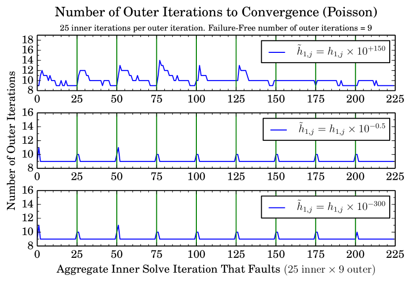
(a) SDC on the first iteration of the Modified Gram-Schmidt loop.

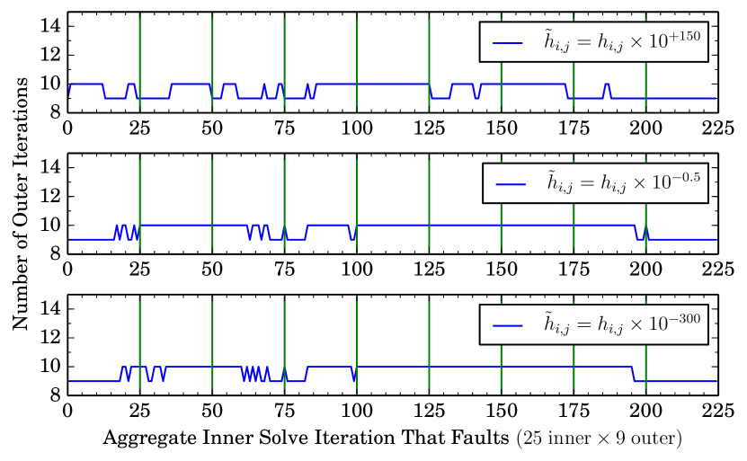
(b) SDC on the last iteration of the Modified Gram-Schmidt loop.

Figure 3: Number of outer iterations required for convergence when solving a Poisson equation given a single SDC event injected in the orthogonalization phase of the inner solve. Vertical bars indicate the start of a new inner solve.

VII-C1 Faulting on the first Modified Gram-Schmidt iteration

In Figure 3(a), we see a large penalty in time to solution for large faults. This is due to making entries in $\boldsymbol{\mathbf{H}}$ that should be zero, clearly nonzero. In contrast, if we only slightly perturb these “near zero” entries (class 2 and 3 errors), we see very little impact on time to solution. The largest increase in outer iterations is two, while the majority of experiments resulted in no increase in time to solution. It should be noted that if our fault detector on $h_{i,j}$ was used, the top plot (large fault) would not be possible.

VII-C2 Faulting on the last Modified Gram-Schmidt iteration

Faulting on the last Modified Gram-Schmidt iteration is much different from faulting on the first for an SPD problem, because the last $h_{i,j}$ entry created in the orthogonalization phase could theoretically be nonzero. From figure 3(b) we see that the worst case is that we incur one additional outer iteration. Considering both faults at the start and end of the MGS process, we see that with our detector we see a maximum increase in outer iterations to be $2$, in contrast if our detector were not used, we see increase in outer iterations of $5$.

VII-D Faulting in a nonsymmetric problem

We now consider a problem that is not symmetric, meaning that all $h_{i,j}$ we perturb may be zero, but could also be nonzero — but each entry in $\boldsymbol{\mathbf{H}}$ is still subject to the bound from Eq. (3). In a failure-free solve FT-GMRES required 28 outer iterations, with each inner solve performing 25 inner iterations. As in our prior analysis, we consider faults in both the first and last iteration of the Modified Gram-Schmidt process.

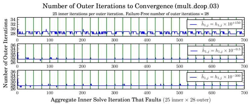
(a) SDC on the first iteration of the Modified Gram-Schmidt loop.

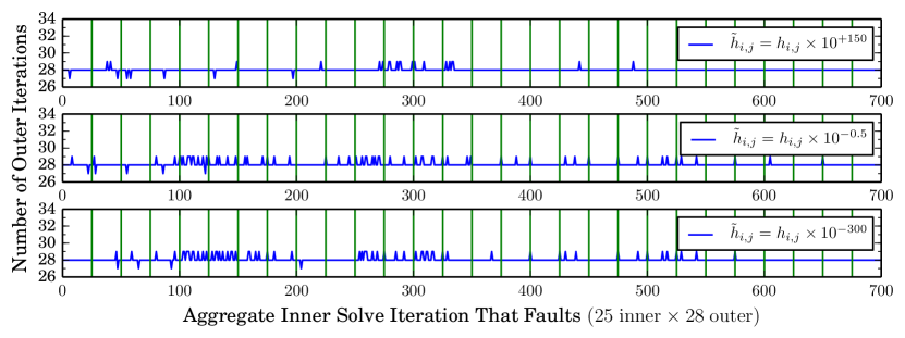
(b) SDC on the last iteration of the Modified Gram-Schmidt loop.

Figure 4: Number of outer iterations required for convergence when solving the mult_dcop_03 system of equations given a single SDC event injected in the orthogonalization phase of the inner solve. Vertical bars indicate the start of a new inner solve.

VII-D1 Faulting on the first Modified Gram-Schmidt iteration

As expected, in Figure 4 we see a very different characteristic for faults on the first MGS iteration. For large faults we see a maximum increase in time to solution to be 2 outer iterations. For small faults, we see that the first iteration of the MGS of the first inner solve is extremely vulnerable to small faults. For class 2 and 3 faults, we see a maximum increase in outer iterations of 4. If we ignore the first 3 iterations of the inner solve we see at most 1 additional outer iteration. The worst-case increase in time to solution actually occurs on the 2^nd inner solve iteration, and we leave to future work’s further analysis of the Arnoldi process to explain this phenomenon. This indicates that additional robustness should be added at the very start of the first inner solve, and we discuss this briefly in our summary.

VII-D2 Faulting on the last Modified Gram-Schmidt iteration

Faulting on the last iteration of the orthogonalization loop again presents a worst case compared to faulting early. That is, by faulting on the last orthogonalization iteration, we see an increase in outer iterations in more cases. We do not the see the sharp increase in iteration count for faults early in the first inner solve iterations. Note, that the first MGS iteration is also the last on the first inner solve iteration, and as stated previously, the first iteration did not exhibit a large increase in iterations.

VII-E Summary of Findings

A common feature seen between both SPD and nonsymmetric solves is that faulting early in the first inner solves’ orthogonalization is universally bad, resulting in a $33\%$ increase in time to solution for the Poisson problem and $14\%$ increase in time to solution for the mult_dcop_03 problem. These percent increases are not general findings, but we believe this characteristic will hold true in most, if not all, cases. This may indicate that additional effort should be expended early in the first inner solve.

VII-E1 Performance Characteristics of GMRES

The amount of work per-iteration of GMRES increases linearly. This is seen in Algorithm 1 in the orthogonalization phase, where the inner loop iterates from 1 to $j$. Adding redundant computation early in the inner solve would have minimal performance impact because the orthogonalization kernel has substantially less work to perform than in latter iterations. If we included additional robustness only on the first invocation of the inner solver, we can mitigate the one edge-case where we see high variability in time to solution. We leave this to future work.

VII-E2 Filtering values is cheap and effective

In all experiments, we find that exploiting the bound on the upper Hessenberg entries is beneficial, and, in doing so, we typically observe one additional outer iteration as the penalty should a single SDC event occur. We believe that this research approach will yield additional invariants that are cheap to evaluate, and that by combining light-weight mechanisms we drastically reduce the damage that SDC can introduce.

VIII Conclusions

In summary, we developed a cheap fault detector for the computational intensive orthogonalization stage of GMRES. We then present the FT-GMRES algorithm, and discuss robustness improvements in the local least squares solve. We then explained how are detector and robustness modifications can be used to limit the amount of error that the inner solve may return.

We presented results from two experiments on common classes of matrices that illustrate that our filtering technique is beneficial, and identified the early stages of the first inner solve as being the most vulnerable. Furthermore, we observe that the inner/outer iteration scheme based on FGMRES is extremely robust to single events of SDC in the orthogonalization phase. We find that this nested approach, even when not coupled with invariant checks can cope with even large perturbations introduced by SDC.

References

- [1] P. G. Bridges, K. B. Ferreira, M. A. Heroux, and M. Hoemmen, “Fault-tolerant linear solvers via selective reliability,” ArXiv e-prints, Jun. 2012.
- [2] Intel, “FDIV replacement program: Description of the flaw,” Jul. 2004.
- [3] Y. Saad, “A flexible inner-outer preconditioned GMRES algorithm,” SIAM J. Sci. Comput., vol. 14, no. 2, pp. 461–469, Mar. 1993.
- [4] M. A. Heroux et al., “An overview of the Trilinos project,” ACM Trans. Math. Softw., vol. 31, no. 3, pp. 397–423, 2005.
- [5] K. Asanovic, R. Bodik, B. C. Catanzaro, J. J. Gebis, P. Husbands, K. Keutzer, D. A. Patterson, W. L. Plishker, J. Shalf, S. W. Williams, and K. A. Yelick, “The Landscape of Parallel Computing Research: A View from Berkeley,” EECS Department, University of California, Berkeley, Tech. Rep. UCB/EECS-2006-183, Dec 2006.
- [6] K. Asanovic, R. Bodik, J. W. Demmel, T. Keaveny, K. Keutzer, J. Kubiatowicz, N. Morgan, D. A. Patterson, K. Sen, J. Wawrzynek, D. Wessel, and K. A. Yelick, “A View of the Parallel Computing Landscape,” Communications of the ACM, vol. 52, no. 10, pp. 56–67, 2009.
- [7] P. M. Kogge et al., “ExaScale Computing Study: Technology Challenges in Achieving Exascale Systems,” University of Notre Dame CSE Department, Tech. Rep. TR-2008-13, September 2008.
- [8] T. Karnik, P. Hazucha, and J. Patel, “Characterization of soft errors caused by single event upsets in CMOS processes,” IEEE Trans. Dependable Secur. Comput., vol. 1, pp. 128–143, April 2004.
- [9] N. Miskov-Zivanov and D. Marculescu, “Soft error rate analysis for sequential circuits,” in Proceedings of the Conference on Design, Automation and Test in Europe, ser. DATE ’07. San Jose, CA, USA: EDA Consortium, 2007, pp. 1436–1441.
- [10] I. S. Haque and V. S. Pande, “Hard data on soft errors: A large-scale assessment of real-world error rates in GPGPU,” in Proceedings of the 2010 10th IEEE/ACM International Conference on Cluster, Cloud and Grid Computing, ser. CCGRID ’10. Washington, DC, USA: IEEE Computer Society, 2010, pp. 691–696.
- [11] D. Lammers, “The era of error-tolerant computing,” IEEE Spectr., vol. 47, no. 11, p. 15, Nov. 2010.
- [12] M. Shantharam, S. Srinivasmurthy, and P. Raghavan, “Characterizing the impact of soft errors on iterative methods in scientific computing,” in Proceedings of the international conference on Supercomputing, ser. ICS ’11. New York, NY, USA: ACM, 2011, pp. 152–161.
- [13] ——, “Fault tolerant preconditioned conjugate gradient for sparse linear system solution,” in Proceedings of the 26th ACM international conference on Supercomputing, ser. ICS ’12. New York, NY, USA: ACM, 2012, pp. 69–78.
- [14] J. Sloan, R. Kumar, and G. Bronevetsky, “Algorithmic approaches to low overhead fault detection for sparse linear algebra,” in Proceedings of the 2012 42nd Annual IEEE/IFIP International Conference on Dependable Systems and Networks (DSN), ser. DSN ’12. Washington, DC, USA: IEEE Computer Society, 2012, pp. 1–12.
- [15] G. Bronevetsky and B. de Supinski, “Soft error vulnerability of iterative linear algebra methods,” in Proceedings of the 22nd annual international conference on Supercomputing, ser. ICS ’08. New York, NY, USA: ACM, 2008, pp. 155–164.
- [16] S. Michalak, A. Dubois, C. Storlie, H. Quinn, W. Rust, D. DuBois, D. Modl, A. Manuzzato, and S. Blanchard, “Assessment of the impact of cosmic-ray-induced neutrons on hardware in the Roadrunner supercomputer,” Device and Materials Reliability, IEEE Transactions on, vol. 12, no. 2, pp. 445–454, 2012.
- [17] E. Mueller and R. Scheichl, “Massively parallel solvers for elliptic PDEs in numerical weather and climate prediction,” ArXiv e-prints, Jun. 2013.
- [18] Z. Chen, “Online-ABFT: an online algorithm based fault tolerance scheme for soft error detection in iterative methods,” in Proceedings of the 18th ACM SIGPLAN symposium on Principles and practice of parallel programming, ser. PPoPP ’13. New York, NY, USA: ACM, 2013, pp. 167–176.
- [19] Y. Saad and M. H. Schultz, “GMRES: A generalized minimal residual algorithm for solving nonsymmetric linear systems,” SIAM J. Sci. Stat. Comput., vol. 7, no. 3, pp. 856–869, Jul. 1986.
- [20] W. E. Arnoldi, “The principle of minimized iterations in the solution of the matrix eigenvalue problem,” Quarterly of Applied Mathematics, vol. 9, pp. 17–29, 1951.
- [21] G. H. Golub and Q. Ye, “Inexact preconditioned conjugate gradient method with inner-outer iteration,” SIAM J. Sci. Comput., vol. 21, pp. 1305–1320, 1999.
- [22] D. B. Szyld and J. A. Vogel, “FQMR: A flexible quasi-minimal residual method with inexact preconditioning,” SIAM J. Sci. Comput., vol. 23, no. 2, pp. 363–380, 2001.
- [23] G. W. Stewart, “Updating a rank-revealing decomposition,” SIAM J. Matrix Anal. Appl., vol. 14, no. 2, pp. 494–499, April 1993.
- [24] T. A. Davis and Y. Hu, “The University of Florida Sparse Matrix Collection,” ACM Transactions on Mathematical Software, vol. 38, no. 1, pp. 1:1–1:25, 2011.