A study of self-consistent Hartree–Fock plus Bardeen–Cooper–Schrieffer calculations with finite-range interactions

Abstract

In this work we test the validity of a Hartree–Fock plus Bardeen–Cooper–Schrieffer model in which a finite-range interaction is used in the two steps of the calculation by comparing the results obtained to those found in a fully self–consistent Hartree–Fock–Bogoliubov calculations using the same interaction. Specifically, we consider the Gogny–type D1S and D1M forces. We study a wide range of spherical nuclei, far from the stability line, in various regions of the nuclear chart, from oxygen to tin isotopes. We calculate various quantities related to the ground state properties of these nuclei, such as binding energies, radii, charge and density distributions and elastic electron scattering cross sections. The pairing effects are studied by direct comparison with the Hartree-Fock results. Despite of its relative simplicity, in most of the cases, our model provides results very close to those of the Hartree–Fock–Bogoliubov calculations, and it reproduces rather well the empirical evidences of pairing effects in the nuclei investigated.

1 Introduction

The study of the structure of nuclei in regions of the nuclear chart which have not yet been experimentally explored can identify new nuclear properties, and deviations from expected behaviours based on previously established rules [1]. Even though great attention has been addressed to the study of the excitation spectrum of these nuclei [2, 3, 4], one should not neglect the observables related to their ground states such as binding energies, proton and neutron densities, and single particle (s.p.) energies.

In nuclei far from the shell closure, the role of the pairing correlations is particularly important. The simplest mean-field approach taking into account these correlations is the Bardeen–Cooper–Schrieffer (BCS) model [5, 6, 7, 8]. This approach is based on a set of s.p. states given as input. By using a pairing nucleon-nucleon interaction, the model generates partial occupation probabilities for each s.p. state. These probabilites are used to evaluate the pairing effects on the various ground state observables.

The first implementations of the BCS model used s.p. wave functions obtained with phenomenological potentials [9, 10, 6]. More recently, also wave functions generated by Hartree-Fock (HF) calculations have been considered [11, 12, 13, 14, 15]. This latter approach is called HF+BCS method. While in this approach the production of the s.p. states and the evaluation of their pairing correlations are treated in two different types of calculations, the two processes are unified in the Hartree–Fock–Bogoliubov (HFB) theory [7].

The two approaches quoted above, HF+BCS and HFB, are mean-field models that make use of effective forces, i.e. forces whose parameters have been chosen to reproduce nuclear properties within mean-field theories. Among these effective forces, the zero-range Skyrme interaction, in various parameterizations, has been widely used in both HF+BCS [11, 12, 13, 14, 15] and HFB [16, 17, 18] calculations. These calculations are not self-consistent since the zero-range character of the Skyrme interaction generates results strongly dependent on the size of the s.p. configuration space, therefore a different zero-range interaction must be used in the pairing channel. The parameters of this zero-range pairing interaction are chosen to reproduce some specific pairing properties within the particular s.p. configuration space used in the calculation.

As widely discussed in the seminal paper of Dechargé and Gogny [19], this is not any more necessary when finite-range interactions are used, because they provide an automatic convergence of the results, once a sufficiently large size of the s.p. configuration space is adopted, and this allows really self-consistent calculations.

There are many examples of HFB calculations carried out with finite-range interactions. In these works the D1 [19], D1S [20, 21, 22, 23], D1M [24] Gogny interactions and the M3Y force [25] have been used. On the other hand, we know only few works where finite-range interactions are used in HF+BCS calculations. This approach has been used by Robledo et al. [11] with the D1 interaction to analyze the octupole excitation in actinide isotopes, and more recently by Than et al. [26] with the D1S and the M3Y interactions to study the inner crust of neutron stars. The purpose of the present article is to explore, and exploit, the features offered by a HF+BCS approach with finite-range interactions. The use of an unique interaction for the HF and pairing calculations offers a large prediction power, and this is associated with the advantage of calculations which are numerically less involved than those of the HFB approach. One of the goals of this article is to test the limits of this self–consistent HF+BCS approximation for studying pairing correlations in regions of the nuclear chart far from the stability line. For this purpose, we compare the results of both HF+BCS and HFB approaches by using the same finite-range effective nucleon-nucleon interaction.

In section 2, we briefly present the basic ideas of our approach, and we describe how we calculate the various observables we have considered in our work. In section 3 we present our results. First we compare the fluctuation of the particle number obtained in our model with that of the HFB to test the validity of our calculations. Then, we discuss the results obtained for binding energies, s.p. properties, proton and neutron root mean square (rms) radii and density distributions. In section 4 we summarize our results and we draw our conclusions.

2 The model

In this section we present the main features of our approach, and describe how we calculate binding energies, radii, and density distributions. The first step of our HF+BCS procedure consists in obtaining the s.p. wave functions $\phi_{i}$ by solving the HF equations [7]

$$-\frac{\hbar^{2}}{2m}\,\nabla^{2}\phi_{i}({\bf r}_{1})\,+\,U({\bf r}_{1})\,\phi_{i}({\bf r}_{1})\,-\,\int{\rm d}^{3}r_{2}\,W({\bf r}_{1},{\bf r}_{2})\,\phi_{i}({\bf r}_{2})\,=\,\epsilon_{i}\,\phi_{i}({\bf r}_{1})\,,$$ (1)

where $m$ is the nucleon mass and $\epsilon_{i}$ the s.p. energy. In the above equation we have indicated the Hartree term as

$$U({\bf r}_{1})\,=\,\int{\rm d}^{3}r_{2}\,V({\bf r}_{1},{\bf r}_{2})\,\sum_{k\leq\epsilon_{F}}|\phi_{k}({\bf r}_{2})|^{2}\,,$$ (2)

and the Fock–Dirac term as

$$W({\bf r}_{1},{\bf r}_{2})\,=\,\sum_{k\leq\epsilon_{F}}\,V({\bf r}_{1},{\bf r}_{2})\,\phi^{*}_{k}({\bf r}_{2})\,\phi_{k}({\bf r}_{1})\,.$$ (3)

Here $\epsilon_{F}$ is the Fermi energy, and $V({\bf r}_{1},{\bf r}_{2})$ the effective nucleon-nucleon interaction.

In this work, we consider only spherical even-even nuclei and solve the HF equations with the method described in Refs. [27, 28]. Once the iteration procedure has reached convergence, the potential terms (2) and (3) are used to generate a set of s.p. wave functions which includes all the states below the Fermi level and a large set of states above it. Each s.p. state $|k\rangle\equiv|\epsilon_{k};n_{k}l_{k}j_{k}m_{k}\rangle$ is characterized by the principal quantum number $n_{k}$, the orbital angular momentum $l_{k}$, the total angular momentum $j_{k}$, its $z$ axis projection $m_{k}$ and, finally, the $2j_{k}+1$ degenerated energy $\epsilon_{k}$. These s.p. wave functions and energies are used to solve the BCS equations.

In the BCS theory the ground state of the system is defined as

$$|{\rm BCS}\rangle\,=\,\prod_{k>0}\left(u_{k}\,+\,v_{k}\,a_{k}^{\dagger}\,a_{\bar{k}}^{\dagger}\right)\,|-\rangle\,,$$ (4)

where $|-\rangle$ is the vacuum, $a_{k}^{\dagger}$ is the creation operator of the state $|k\rangle$, $a_{\bar{k}}^{\dagger}$ is the creation operator of the state

$$|\bar{k}\rangle\,=\,(-1)^{j_{k}-m_{k}}\,|-k\rangle\,=\,(-1)^{j_{k}-m_{k}}\,|\epsilon_{k};n_{k}l_{k}j_{k}-m_{k}\rangle\,,$$ (5)

and $|v_{k}|^{2}$ the probability that the state $|k\rangle$ is occupied, and is related to $u_{k}$ by the condition

$$|u_{k}|^{2}+|v_{k}|^{2}=1\,.$$ (6)

It is worth to point out that $u_{\bar{k}}=u_{k}$ and $v_{\bar{k}}=-v_{k}$.

The BCS state defined in equation (4) is not an eigenstate of the particle number operator. For this reason, the BCS equations are obtained by applying the variational principle to the expectation value of the operator

$$\mathcal{H}\,=\,H\,-\,\lambda N\,,$$ (7)

where $H$ is the traditional nuclear hamiltonian, $N$ is the particle number operator and $\lambda$ is a Lagrange multiplier. The parameters to be changed in the variational procedure are the $v_{k}$ and $u_{k}$ coefficients. The application of the variational principle leads to solve the set of equations

$$\left(u_{k}^{2}-v_{k}^{2}\right)\,\Delta_{k}\,=\,2\,u_{k}\,v_{k}\,\eta_{k}\,,$$ (8)

where

$$\Delta_{k}\,=\,-\frac{1}{{\widehat{j}}_{k}}\sum_{i}{\widehat{j}}_{i}\,u_{i}\,v_{i}\,\langle ii\,0|{V}|kk\,0\rangle\,,$$ (9)

and

$$\eta_{k}\,=\,\langle k|T|k\rangle\,-\,\lambda\,.$$ (10)

In the last definition, we have indicated with $T$ the kinetic energy operator and we dropped a renormalization term [8]. In the above equations, for the indexes indicating angular momentum eigenvalues, we have used the symbol $\widehat{j}=\sqrt{2j+1}$. The matrix element of the interaction in equation (9) indicates that the s.p. wave functions are coupled to global angular momentum zero.

The solution of the BCS equations, Eqs. (8)-(10), provides the values of $v_{k}$ and $u_{k}$ for each s.p. state included in the configuration space. The knowledge of $v_{k}$ and $u_{k}$ and $\phi_{k}$ allows the evaluation of the expectation values of various ground state quantities related to the BCS ground state.

We have considered the particle number fluctuation index which is defined as

$$\langle(\Delta N)^{2}\rangle\,=\,\langle{\rm BCS}|\hat{N}^{2}|{\rm BCS}\rangle\,-\,\langle{\rm BCS}|\hat{N}|{\rm BCS}\rangle^{2}\,=\,4\sum_{k}(2j_{k}+1)\,u_{k}\,v_{k}\,.$$ (11)

The value of this quantity is directly related to the relevance of the pairing effects. In what follows, we indicate as $\langle(\Delta N)^{2}\rangle_{\rm p}$ and $\langle(\Delta N)^{2}\rangle_{\rm n}$ the values obtained when the sum of equation (11) is restricted to proton or neutron s.p. states, respectively. In the next section we shall compare the values obtained in our HF+BCS approach with those of the HFB calculation.

We calculate the quasi-particle energy as

$$E_{k}\equiv\sqrt{\epsilon_{k}^{2}+\Delta_{k}^{2}}\,,$$ (12)

and the global energy of the HF+BCS ground state as

$$E\,=\,\frac{1}{2}\sum_{k}(2j_{k}+1)\,\left[v_{k}^{2}(\epsilon_{k}+\langle k|T|k\rangle)\,-\,u_{k}\,v_{k}\,\Delta_{k}\right]\,.$$ (13)

We evaluate also the HF+BCS matter densities as

$$\rho(r)\,=\,\sum_{k}v_{k}^{2}|\phi_{k}({\bf r})|^{2}\,=\,\frac{1}{4\pi}\sum_{k}(2j_{k}+1)\,v_{k}^{2}|R_{k}(r)|^{2}\,,$$ (14)

where $R_{k}$ denotes the radial part of the s.p. wave function normalized as

$$\int_{0}^{\infty}\,r^{2}|R_{k}(r)|^{2}\,dr=1\,\,.$$ (15)

With the proper limitations in the sum of equation (14) we calculate the proton and neutron density distributions. The charge distribution is obtained by folding the proton distribution with the nucleon electromagnetic form factor. By using the matter distributions we determine the rms radii as

$$R_{\alpha}\,=\,\langle r^{2}\rangle^{1/2}_{\alpha}\,=\,\left[\frac{\displaystyle\int_{0}^{\infty}r^{4}\,\rho_{\alpha}(r)\,{\rm d}r}{\displaystyle\int_{0}^{\infty}r^{2}\rho_{\alpha}(r)\,{\rm d}r}\right]^{1/2}\,,$$ (16)

where $\alpha$=p indicates protons, and $\alpha$=n neutrons.

The HF+BCS densities differ from the HF ones because of the changes in the occupation probabilities induced by the BCS calculation. This is a remarkable difference with respect to HFB where both s. p. wave functions and their occupation probabilities are obtained in a self-consistent way.

As already pointed out in the introduction our HF+BCS calculations have been carried out by using an effective finite-range interaction of Gogny type [19, 20], which can be expressed as a sum of a central, $V_{\rm C}$, a spin-orbit, $V_{\rm SO}$, and a density dependent, $V_{\rm DD}$, term

$$V(1,2)\,=\,V_{\rm C}(1,2)\,+\,V_{\rm SO}(1,2)\,+\,V_{\rm DD}(1,2)\,.$$ (17)

Only the central term has a finite range. The other two terms are of zero-range type, and have the same expressions used in Skyrme interactions. While in the HF calculations the full expression of the interaction (17) is used, in the BCS calculations we consider only the central, finite-range term. This is the procedure commonly adopted in the pairing sector of the HFB calculations when Gogny type interactions are used [19, 20, 29].

Our calculations have been carried out with two parametrizations of the Gogny force. A first one is the more traditional D1S [20], well known and widely used in the literature. The second one is the more recent D1M [24] built as a correction of the D1S force to have a realistic behaviour of the neutron matter equation of state above saturation densities.

We have already remarked that the BCS calculations are carried out after the s.p. configuration space has been chosen. The size of this space should be large enough to ensure the stability of the results. This implies that some of the s.p. states, obviously above the Fermi energy, lie in the continuum. To the best of our knowledge, there is not a BCS approach treating the continuum part of the configuration space without approximation, contrary to what has been done with the Random Phase Approximation [30]. We have adopted a procedure where the continuum part of the s.p. configuration space is conveniently discretised [27, 28, 31]. Specifically, we have chosen a box of radius $R_{\rm max}=4\,r_{0}\,A^{1/3}$, with $r_{0}=1.2$ fm, where the energy levels were calculated with the HF potential.

From the numerical point of view, the sum on the s.p. states in equation (9) is automatically limited when a finite-range interaction is used. In our BCS calculations, we have included all states with energy below 10 MeV for all nuclei studied. We have checked that this guarantees the convergence of the BCS energy with an order of accuracy in the keV range.

3 Results

We have applied our HF+BCS approach to study oxygen, calcium, nickel, zirconium and tin isotope chains. We have also investigated the $N=40$ and $N=50$ isotone chains. All nuclei studied are of even–even type. In some cases we compare our results with those obtained in HFB calculations [29, 21].

3.1 Particle number fluctuation

In this section we compare the pairing correlations described by our HF+BCS approach with those obtained by the HFB model. We conduct this investigation by considering the particle number fluctuation index $\langle(\Delta N)^{2}\rangle$, defined in equation (11), a quantity particularly sensitive to the pairing correlations. We compare the results obtained with our HF+BCS model with those obtained in HFB calculations by using the same interaction.

We start our analysis by investigating the chains of nuclei where one type of nucleons fills completely all the s.p. levels below the Fermi surface. For these nucleons the pairing effects are negligible, therefore $\langle(\Delta N)^{2}\rangle_{\alpha}$, $\alpha\equiv{\rm p}$ or n, is zero.

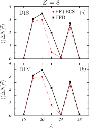
Figure 1: (Color on line) Values of the particle fluctuation index $\langle(\Delta N)^{2}\rangle$ in oxygen isotopes obtained in HF+BCS (red dots) and HFB (black squares) calculations carried out with the D1S, panel (a), and D1M, panel (b), Gogny interactions. The lines are drawn to guide the eyes. In this case only neutrons contribute, therefore $\langle(\Delta N)^{2}\rangle$$\equiv$$\langle(\Delta N)^{2}\rangle_{\rm n}$.

We show in figure 1 the $\langle(\Delta N)^{2}\rangle$ values, as a function of the mass number, for a set of oxygen isotopes calculated with the D1S and D1M interactions, panel (a) and (b), respectively. For these isotopes $\langle(\Delta N)^{2}\rangle_{\rm p}$ is zero, since $Z=8$ closes a shell. In the figure, the red dots show our HF+BCS results while the black squares those obtained in HFB calculations. The lines have been drawn to guide the eyes. We observe that the two interactions produce very similar results. For this reason, in the remaining part of this section we shall present only the values found with the D1M interaction, unless explicitly stated.

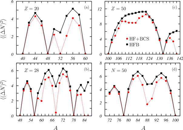
Figure 2: (Color on line) Values of $\langle(\Delta N)^{2}\rangle$ for calcium (a), nickel (b), and tin (c) isotopes and $N=50$ isotones (d) obtained in HF+BCS (red circles) and HFB (black squares) calculations with the Gogny D1M interaction. In panels (a)-(c) only neutrons contribute and $\langle(\Delta N)^{2}\rangle$$\equiv$$\langle(\Delta N)^{2}\rangle_{\rm n}$. In panel (d) only protons contribute and $\langle(\Delta N)^{2}\rangle$$\equiv$$\langle(\Delta N)^{2}\rangle_{\rm p}$.

Together with the oxygen results of figure 1 we discuss also the results shown in figure 2 for calcium, nickel and tin isotopes and a set of isotones with $N=50$. The behaviour of the results of the two types of calculations is very similar in all the nuclear chains we have considered. However, all the $\langle(\Delta N)^{2}\rangle$ values obtained with our HF+BCS approach are smaller, or at most equal, than those of the HFB calculations. This is a clear indication that, for a given interaction, the amount of pairing correlations generated by the HF+BCS approach is smaller than that produced by the HFB calculations.

In the panel (a) of figure 2, where the results relative to the calcium isotopes are shown, the case of the ⁵²Ca nucleus is remarkable. In this nucleus our HF+BCS model predicts zero pairing, contrary to the result obtained in the HFB calculation. In the HF description of the ⁵²Ca nucleus, the neutron 2p_3/2 s.p. state at -5.56 MeV is fully occupied, and the next two s.p. levels are the 2p_1/2 state, whose energy is 2.3 MeV larger, and the 1f_5/2 state which has an even larger energy, 3.6 MeV. These energy differences are large enough to hinder, in BCS calculations, the mixing between these three s.p. levels. On the contrary, the HFB calculations are more flexible and generate pairing effects even between these so well separated s.p. states. As we are going to comment in the following, we have verified that the source of all the remarkable deviations between the HFB and our HF+BCS results is due to situations rather similar to the one just discussed.

Panel (b) shows the results obtained for the nickel isotopes, where the situation of the ⁶⁰Ni nucleus is remarkable. This nucleus has the same neutron structure as the ⁵²Ca nucleus but the $\langle(\Delta N)^{2}\rangle_{\rm n}$ value obtained in the HF+BCS calculation shows a clear difference with respect to that of the HFB calculation. In this case, the pairing effects are not zero as in the ⁵²Ca case, even though they are noticeably smaller than those generated by the HFB calculation.

The discrepancy between the two calculations is evident for the ⁸⁴Ni and ⁸⁶Ni nuclei where all the HF s.p. states up to the 2d_5/2 and 3s_1/2 levels, respectively, are completely filled. The energy differences with respect to the next levels are about 1-2 MeV, and our BCS calculations are unable to generate pairing correlations between these states.

The results of panel (c) relative to the tin isotopes show differences between the two calculations in a relatively large band of isotopes from ¹¹²Sn up to ¹²⁴Sn. These effects have consequences also on the global energies of these isotopes, and we shall discuss in detail their source in the next section. For larger values of the neutron number, we observe that larges differences appear for the ¹³⁸Sn and ¹⁴⁰Sn nuclei. In the last case neutrons occupy all the s.p. states up to the 2f_7/2 level, but the closest s.p. states above it are situated at energies too large to allow the BCS calculations to generate enough pairing.

In the panel (d) of the figure we show the $\langle(\Delta N)^{2}\rangle_{\rm p}$ values for a set of isotones with $N=50$. The agreement between the results of the two approaches is quite good, with the exceptions of the ⁸⁸Sr and ⁹⁰Zr nuclei where the pairing effects in our HF+BCS model are smaller than those found in the HFB calculations. In the HF description of these two nuclei, the proton levels are completely filled up to the 1f_5/2 state in ⁸⁸Sr, and up to the 2p_1/2 state in ⁹⁰Zr. These results show, again, the difficulty of the HF+BCS approach to generate configuration mixing analogous to that of the HFB model.

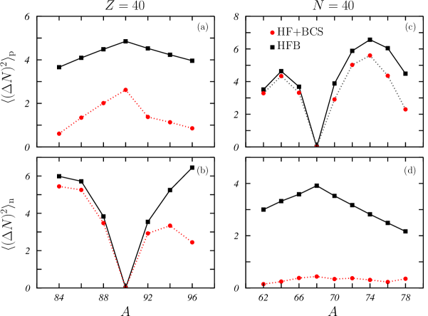
Figure 3: (Color on line) Values of $\langle(\Delta N)^{2}\rangle_{\rm p}$ (upper panels) and $\langle(\Delta N)^{2}\rangle_{\rm n}$ (lower panels) for $Z=40$ isotopes (left panels) and $N=40$ isotones (rigth panels). The meaning of the symbols is the same as in figure 2.

We show in figure 3 the $\langle(\Delta N)^{2}\rangle$ values for nuclei where, in HF model, both proton and neutron levels are open. In the panels (a) and (b) we show, respectively, the $\langle(\Delta N)^{2}\rangle_{\rm p}$ and the $\langle(\Delta N)^{2}\rangle_{\rm n}$ values for a set of zirconium isotopes, $Z=40$, and in the other two panels we show the same quantities calculated for a set of $N=40$ isotones. Before entering in a detailed discussion of the results, we want to remark that the HFB results are always larger, or at most equal, to those of the HF+BCS calculation.

In a HF picture of zirconium isotopes, the protons fill completely all the s.p. levels up to the 2p_1/2 state. The pairing interaction generates a mixing of the 1f_5/2, 2p_3/2, 2p_1/2 and 1g_9/2 proton s.p. levels as the results shown in the panel (a) indicate. The behaviour of the $\langle(\Delta N)^{2}\rangle_{\rm p}$ values is rather flat, as we expected because the proton number does not change. The HF+BCS and HFB results show similar behaviour but rather different size. We find an analogous situation in the $\langle(\Delta N)^{2}\rangle_{\rm n}$ results obtained for the $N=40$ isotones, as it is shown in the panel (d) of the same figure. Also in this case the behaviour of the $\langle(\Delta N)^{2}\rangle_{\rm n}$ values is rather flat, and the values of the HF+BCS results are much smaller than those obtained in HFB calculations. The results of panel (a) and (d) indicate that the $\langle(\Delta N)^{2}\rangle$ values of the HF+BCS calculations are noticeably smaller than those obtained in HFB calculations when the number of one type of nucleons is 40. We point out that these are the largest differences between HF+BCS and HFB results we have encountered in our investigation.

The situation is completely different for the other type of nucleons, as it is shown by the results presented in the panels (b) and (c) of the figure. In both cases the behaviour is not flat, furthermore, the differences between the $\langle(\Delta N)^{2}\rangle$ generated by the two types of calculation are not as large as in the previously discussed cases.

In panel (b) we show the $\langle(\Delta N)^{2}\rangle_{\rm n}$ values for the zirconium isotopes. We observe that both calculations recognize the shell closure for $N=50$, corresponding to the ⁹⁰Zr isotope. The situation is analogous for the results of panel (c) related to the $N=40$ isotones where the closure for the 28 protons, corresponding to the ⁶⁸Ni nucleus, is well recognized by the two types of calculations.

3.2 Observables

In this section we present the results of our study of the pairing effects on binding energies, and charge and matter density distributions. We use the latter quantities to calculate rms radii and elastic electron scattering cross sections. Our investigation has been conducted by using both D1S and D1M interactions. Since the two interactions provide similar results, to simplify the discussion, we present only those obtained with the D1M interaction.

3.2.1 Binding energies.

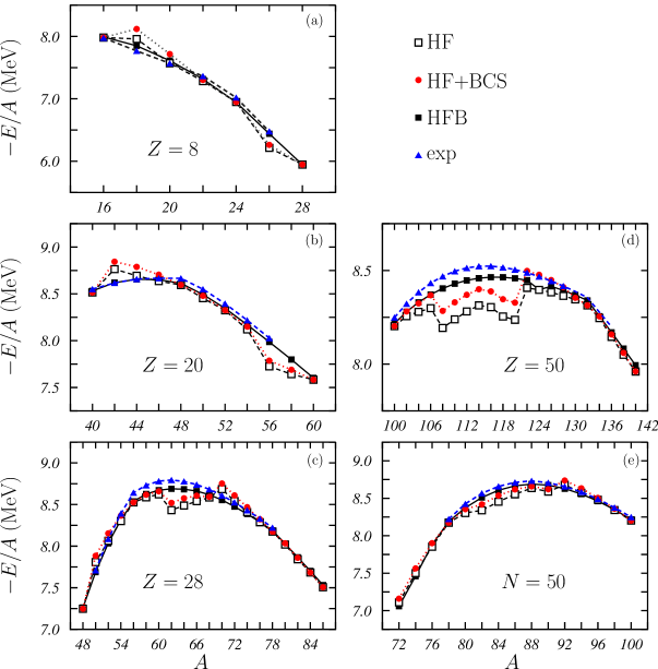
Figure 4: (Color on line) Binding energies per nucleon for oxygen (a), calcium (b), nickel (c), and tin (d) isotopes and $N=50$ isotones (e) calculated with the Gogny D1M in HF+BCS (red circles), HFB (black squares) and HF (open squares) models. The blue triangles show the experimental values taken from [32]. The lines have been drawn to guide the eyes.

We show in figure 4 the binding energies per nucleon for oxygen, calcium, nickel and tin isotope chains and for a set of $N=50$ isotones. The red circles and the black squares indicate the HF+BCS and HFB results, respectively, and the empty squares those of the HF calculation, where the pairing is not considered. The blue triangles show the experimental values taken from Ref. [32]. In this figure all the scales of the y axes have been chosen to emphasize the differences between the results of the various calculations whose maximum relative value reaches 2%.

In all the panels we observe that the behaviour of the HFB results is quite smooth, while that of the HF+BCS calculations is less regular. In general, the HF+BCS results are closer to the experimental values than HF results except for ¹⁸O, ²⁰O, ⁴²Ca, ⁴⁴Ca,⁵⁰Ni, ⁷⁰Ni, ⁷²Ni and ⁹²Mo. Furthermore, HFB calculations are in better agreement with the experiment than our HF+BCS calculations that show again the effects of a smaller pairing.

By considering in more detail the results shown in figure 4, we observe that our HF+BCS nickel binding energies, shown in the panel (c) have two discontinuity points related to the ⁶²Ni and ⁷⁰Ni nuclei. The discontinuities in our HF+BCS results are even more evident in the panel (d) where the binding energies of the tin isotopes are presented. In this case, the HFB and the HF+BCS values are in excellent agreement up to $A=106$. After that, all the HF+BCS binding energies of the isotopes going from ¹⁰⁸Sn up to ¹²⁰Sn are smaller than those of the HFB calculations. We observe another discontinuity in coincidence with the ¹²²Sn isotope, where HF+BCS binding energy is larger than that obtained in the HFB calculation. This trend continues up to the ¹²⁶Sn nucleus, and, then, the agreement between the results of the two calculations becomes again excellent.

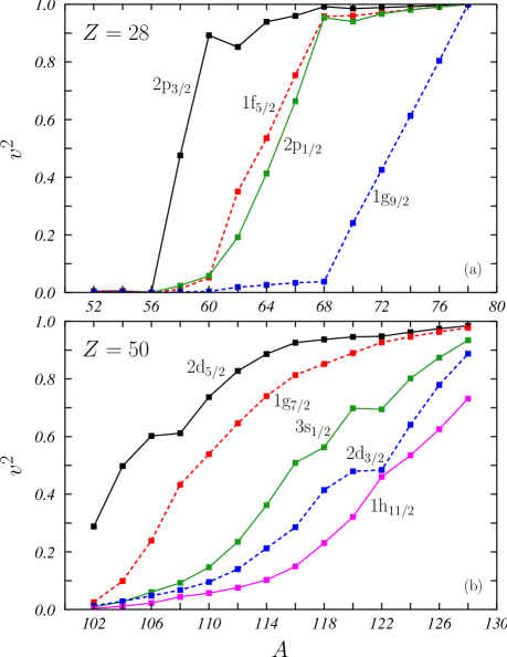
Figure 5: (Color on line) Occupation probabilities $v^{2}$ of different neutron s. p. levels for nickel (a) and tin (b) isotopes obtained in HF+BCS calculations with the D1M Gogny interaction.

We have investigated the reason of this behaviour. After having excluded any numerical instability of our calculations, we focused our attention to the occupation of the various s.p. levels. As example, we show in figure 5 the HF+BCS occupation probabilities $v^{2}$ for various neutron s.p. levels of the nickel and tin isotopes around the Fermi level. In the nickel isotope chain, panel (a), we observe a change in the behaviour of the occupation probability for the 2p_3/2 state at $A=60$ and for the 1f_5/2 and 2p_1/2 states at $A=68$. In the case of the tin isotopes, panel (b), we also observe some discontinuities in the trend of the $v^{2}$ values. This happens at $A=106$ for the 2d_5/2 state, and at $A=120$ for the 3s_1/2 and 2d_3/2 states. In these cases, the values of $v^{2}$ remain almost constant for the next isotope and, after that, they start again to rise.

These behaviours of the occupation probabilities $v^{2}$ are related to the energy of the s.p. HF levels. For example, from ⁵⁸Ni to ⁶⁴Ni, the energy of the neutron 2p_3/2 and 2p_1/2 states change by $-200$ keV at most. However, that of the 1f_5/2 state is reduced by more than 600 keV from ⁶⁰Ni to ⁶²Ni, becoming almost constant afterwards. This provokes an enhancement of the occupation probability of the 1f_5/2 state and, as a consequence, that of the 2p_3/2 is reduced. It is precisely between these two nuclei where the larger discrepancy between HF+BCS and HFB binding energies is observed. Similar arguments apply in the other cases above mentioned. This allows us to understand the discontinuities pointed out in the $\langle(\Delta N)^{2}\rangle_{\rm p}$ results of the panel (c) of figure 2 and of those we have observed in the panels (c) and (d) of figure 4. These results indicate that our HF+BCS approach is less flexible in handling the filling of the s.p. levels than the HFB method.

The comparison of our HF+BCS results with the experimental data, taken from the compilation of Ref. [32], and indicated with blue triangles in figure 4, is quite satisfactory. In panel (a), we observe some differences with the experimental data in ¹⁸O and ²⁰O that are both overbound, and in ²⁶O which is, on the opposite, underbound. For the calcium isotopes, panel (b), our HF+BCS results overbind ⁴²Ca and ⁴⁴Ca. In the nickel chain, panel (c), we find a small underbinding in the isotopes between the ⁵⁶Ni and ⁶⁸Ni, while ⁵⁰Ni, ⁷⁰Ni and ⁷²Ni are overbound. In the panel (d) we observe that all the tin isotopes with $A<122$ are underbound, while a good agreement with the experimental data is found for the heavier isotopes. We observe an even better agreement in the $N=50$ isotone chain shown in panel (e). The maximum relative difference we found between the experimental data and our HF+BCS results is of about the 3%.

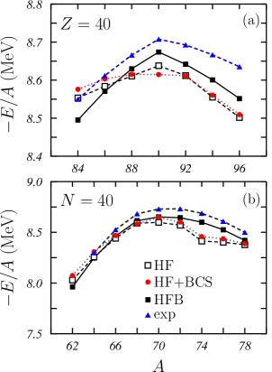
Figure 6: (Color on line) Binding energies for $Z=40$ isotopes (a) and $N=40$ isotones (b). The meaning of the symbols is the same as in figure 4.

We have calculated also the binding energies for nuclei where both proton and neutron shells are open. The results for the $Z=40$ isotope chain, and for the $N=40$ isotone chain are shown in figure 6. In these chains the ⁹⁰Zr and ⁶⁸Ni nuclei have closed the neutron and proton shells, respectively.

The results shown in this figure confirm the findings and the observations we presented in the study of figure 4. We find good agreement between HF+BCS and HFB results. The maximum relative difference is 1.7%, found in the case of the ⁷⁴Se nucleus. Also the agreement with the experimental data is quite good. In this case, the largest discrepancy we observe is of about 2%, always in ⁷⁴Se. The effects of the pairing are rather small. The differences between HF+BCS and HF results are below 0.5%.

3.2.2 Radii.

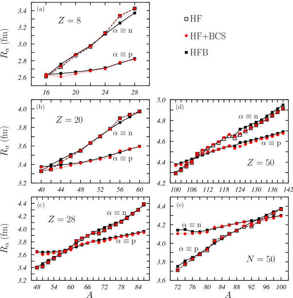
Figure 7: (Color on line) Proton, $R_{\rm p}$, and neutron, $R_{\rm n}$, rms radii for oxygen (a), calcium (b), nickel (c), and tin (d) isotopes and $N=50$ isotones (e). The red circles indicate the HF+BCS results, the black and open squares those obtained in HFB and HF calculations, respectively. All the calculations have been carried out with the Gogny D1M interaction.

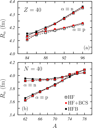
Figure 8: (Color on line) The same as in figure 7 for $Z=40$ isotopes (a) and $N=40$ isotones (b).

We show in Figs. 7 and 8 the proton, $R_{\rm p}$, and neutron, $R_{\rm n}$, rms radii for the various isotopes and isotones under investigation. The red circles show the results obtained in HF+BCS calculations, the black and empty squares those obtained, respectively, by using the HFB and HF approaches. The results presented in Figs. 7 and 8 have been obtained with the D1M Gogny interaction. In the cases where the shells are closed, $Z=8$, 20, 28 and 50 for protons and $N=50$ for the neutrons, HF and HF+BCS calculations give the same results, therefore we do not show the empty squares of the HF results. The scales of the y axes have been chosen to emphasize the differences between the various results.

We observe in Figs. 7 and 8 a remarkable agreement between the HFB and HF+BCS results. We find a maximum relative difference of 1.5% for $R_{\rm p}$ in ¹⁸O, and of 1.9% for $R_{\rm n}$ in ²⁶O. The comparison with the HF results indicates that the pairing effects on the rms radii, are rather small. The relative differences are smaller than 0.8%.

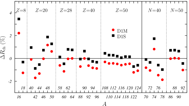
Figure 9: (Color on line) Relative differences, as given by equation (18), between HF+BCS results obtained with D1M (red points) and D1S (black squares) interactions and the experimental values taken from Ref. [33].

In order to compare our results with the experiment, we extract charge radii from the charge densities which we obtain by folding the corresponding proton densities with a dipole form factor. In figure 9 we show the relative differences, multiplied by 100, between the results of our HF+BCS calculations and the experimental radii taken from the compilation of Ref. [33]:

$$\Delta R_{\rm ch}(\%)\,=\,100\,\,\displaystyle\frac{R^{\rm HF+BCS}_{\rm ch}-R^{\rm exp}_{\rm ch}}{R^{\rm exp}_{\rm ch}}\,.$$ (18)

In this figure we present the results only for those nuclei where experimental data are available. We indicate with the red points the results obtained with the D1M interaction, and with the black squares those obtained with the D1S force. All the relative differences are within the 2%, with the only exception of the ¹⁶O, where we found 2.2% for the D1M interaction and 3.4% for the D1S force. We notice that the radii obtained with the D1S force are always larger than those obtained with the D1M interaction.

We expected pairing effects on the charge rms radii to be different from zero only for the nuclei with $Z=40$ and $N=40$ and 50, where the proton s.p. levels in HF description are not completely occupied. Even in these cases, they are rather small. We observe relative differences between the radii calculated with HF+BCS and HF smaller than 0.3%.

3.2.3 Density distributions and electron scattering cross sections.

We conclude our investigation by studying the effects of the pairing on the density distributions of some selected nuclei. The computational technique we use to solve the HFB equations [34] does not provide us with wave functions, therefore we do not compare our results with those of HFB model.

The first case we discuss is that of two $N=20$ isotones, ³⁶S and ³⁴Si. In these nuclei the neutrons fill completely the s.p. states up to the 1d_3/2 level, therefore the pairing effects are present only in the proton sector, and we expect the proton density distributions to be sensitive to these effects. The interest in these two nuclei has been raised by the fact that some calculations [35, 36] indicate ³⁴Si as a good candidate to be a nucleus with bubble density profile, i. e. with a large depletion in its central part. An experiment has been proposed by the collaboration GRETINA [37] at the Lawrence Berkeley National Laboratory, to produce the unstable ³⁴Si nucleus and measure its proton density by means of one-proton knock-out reaction in combination with a gamma spectrometer [38].

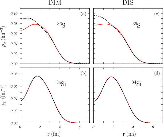
Figure 10: (Color on line) Proton densities distributions for ³⁴Si and for ³⁶S calculated in the HF (dashed black lines) and HF+BCS (solid red lines) approaches. The densities of the panels (a) and (b) have been obtained with the Gogny D1M interaction, and those of the panels (c) and (d) with the D1S interaction.

We present in figure 10 the proton densities of these two nuclei obtained by using the D1M and D1S interactions. The full red lines indicate the results obtained in HF+BCS calculations, while the dashed black lines those of the HF calculations. Our results confirm the findings of Refs. [35, 36] and indicate that the proton density of ³⁴Si has a bubble structure. In our density distributions the pairing effects are large in ³⁶S, but negligible in ³⁴Si, independently of the interaction used in the calculation.

These results are in agreement with those of Ref. [36] where a Skyrme SLy4 force has been used, together with various pairing forces. The study of Grasso et al. [36] concluded that the very large energy gap for $Z=14$, due to the filling of the 1d_5/2 proton s.p. state, prevents pairing from being relevant in ³⁴Si, contrary to what happens in ³⁶S. This occurs also in our HF+BCS calculations, where the pairing effects strongly deplete the central part of the ³⁶S proton distributions. In this nucleus we obtain a small bubble behaviour when the D1M interaction is used. This detail disagrees with the results of Nakada et al. [35] who found, with the D1M interaction, a behaviour of the proton density more similar to the result we obtain with the D1S interaction (see panel (c)).

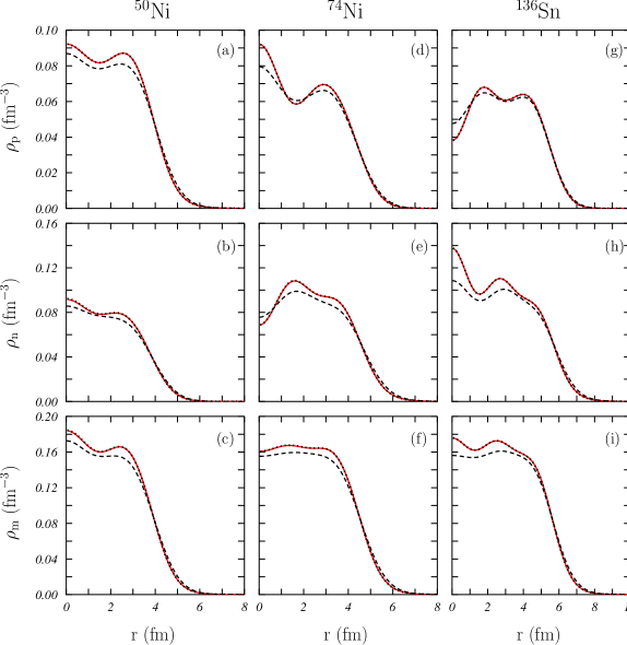
Figure 11: (Color on line) Proton, $\rho_{\rm p}$, neutron, $\rho_{\rm n}$ and matter, $\rho_{\rm m}$, density distributions for the ⁵⁰Ni, ⁷⁴Ni and ¹³⁶Sn nuclei obtained by using the Gogny D1M interaction in HF (dotted black lines) and HF+BCS (solid red lines) calculations. We also show the HF+BCS results (dashed black lines) of Ref. [39] obtained with a Skyrme Sly4 force.

With the purpose of comparing our results with those of similar calculations done with different interactions, we have evaluated the proton, neutron and matter density distributions of the ⁵⁰Ni, ⁷⁴Ni and ¹³⁶Sn nuclei. In figure 11 we compare our results, shown by full red lines, with those obtained in Ref. [39] by using the SLy4 Skyrme interaction. These latter results are indicated in the figure by dashed black lines. The agreement between our results and those obtained with the Skyrme interaction is reasonably good especially in the surface region. In this figure, the dotted black lines indicate the densities obtained in HF calculations. In all the cases, these densities are almost coincident with the HF+BCS results. In the nuclei we consider in the figure, pairing effects should appear in the neutron and, therefore, matter distributions. However, in these cases, the open neutron shells, 1f_7/2 in ⁵⁰Ni, 1g_9/2 in ⁷⁴Ni and 2f_7/2 in ¹³⁶Sn, are rather separated in energy (about 7, 5 and 3 MeV, respectively) with respect to the other open shells just above the Fermi surface. Because of this large energy separation the pairing effects on the densities are negligible. As a final remark on this figure, we observe that the large fluctuations in the nuclear interior shown by proton and neutron densities are smoothed out in the matter distributions which show a flatter behaviour.

As it is well known, the HF+BCS calculations may not be feasible for nuclei with a large neutron excess due to the appearance of an unphysical gas of neutrons around the nucleus. This spurious effect was observed by Dobaczewski et al[40] in HF+BCS calculations for ¹⁵⁰Sn, performed with zero-range interactions. We have controlled that our results did not show this spurious effect.

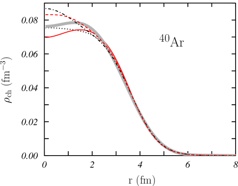
Figure 12: (Color on line) Charge density distribution of the nucleus ⁴⁰Ar obtained in HF with the D1M (dashed red line) and D1S (dashed-dotted black line) interactions and HF+BCS with D1M (solid red line) and D1S (dotted black line) interactions, compared with the experimental distribution [44] (thick gray line).

The nucleus ⁴⁰Ar is quite interesting because is the fundamental ingredient of liquid argon detectors used in the physics of the neutrinos and of rare events [41, 42, 43]. From the nuclear structure point of view the ⁴⁰Ar is characterised by the fact that it has open shells in both proton and neutron sectors. The neutron shell that is open is the 1f_7/2 level. As we have already pointed out for the case of the ⁵⁰Ni nucleus, the energy difference between this state and the neighbouring ones is so large that pairing effects result to be negligible. For this reason we expect the pairing effects to be relevant only on the proton distribution. In figure 12 we show the charge densities obtained in HF calculations with D1M (dashed red line) and D1S (dashed-dotted black line) interactions and those obtained with the HF+BCS approach with D1M (solid red line) and D1S (dotted black line) interactions. The thick grey line shows the empirical charge density distribution [44]. All the calculations reproduce rather well the empirical distribution at the surface. The differences appear in the nuclear centre where the HF results rise continuously while the empirical distribution shows a slightly decreasing behaviour. The pairing modifies the HF densities in the right direction, producing, in the case of the D1M interaction, the depletion at the centre shown by the experiment.

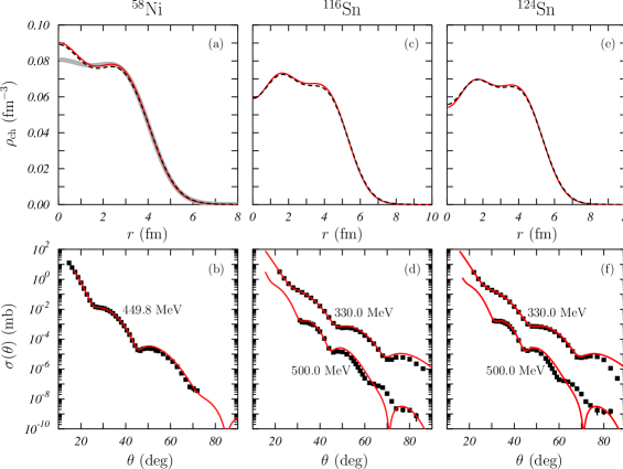
Figure 13: (Color on line) Upper panels: Charge densities for ⁵⁸Ni, ¹¹⁶Sn and ¹²⁴Sn nuclei obtained in HF+BCS calculations by using the D1M (solid red lines) and D1S (dashed black lines) interactions. The thick gray line in panel (a) is the empirical charge density [44]. Lower panels: Elastic electron scattering cross sections for the same nuclei calculated with the HF+BCS charge densities obtained by using the D1M interaction and compared with the experimental results [47, 48, 49]. In each panel the electron energies are indicated.

To test the validity of our approach in the description of the density distributions, we use them to calculate elastic electron scattering cross sections in distorted wave Born approximation [45, 46]. We compare them with experimental data which are available for some of the open shell nuclei we have studied so far. In the upper panels of figure 13 we show the charge densities obtained with the D1M and D1S interactions, indicated, respectively, by the full red and dashed black lines, for ⁵⁸Ni, ¹¹⁶Sn and ¹²⁴Sn. In the panel (a) of the figure we show with a thick gray line the empirical charge density [44].

In these nuclei the proton levels are completely filled, therefore the pairing effects on the charge distributions are very small. The HF density distributions almost coincide with those obtained in HF+BCS calculations. Also the differences between the results of the calculations done with different interactions are rather small, as we show in the upper panels of figure 13.

The elastic electron scattering cross sections shown in the lower panels of the figure have been calculated by using the charge densities obtained with the D1M interaction. Our results describe rather well the experimental data of Refs. [47, 48, 49] for the three nuclei considered. The agreement is particularly good for the ⁵⁸Ni nucleus, panel (b).

For ¹¹⁶Sn and ¹²⁴Sn nuclei, the agreement is very good for the data taken at 330.0 MeV, and it is slightly worse for those taken at 500.0 MeV for scattering angles larger than 50 degrees. The increasing resolution power of the probe emphasises the differences with the experimental charge distributions, differences which we expect to show up mainly in the nuclear interior [45, 46].

4 Summary and conclusions

We have developed a fully self-consistent HF+BCS approach where the same finite-range interaction is used in the two steps of the process, first the HF calculation generating the set of s.p. wave functions and energy, and, second, the BCS calculation taking care of the pairing correlations between these s.p. states. Since the interaction has a finite-range, we obtain a natural convergence of the BCS results once the dimension of the s.p. configuration space have reached a certain size. In our calculations we use two interactions of Gogny type, the D1M and D1S forces.

The motivation of our work is to construct a parameter free computational scheme which can be applied to investigate all the regions of the nuclear chart, therefore, with a large prediction power. Our HF+BCS approach is competitive with the HFB model, which is more elaborated from both the theoretical and computational points of view. One of the main purposes of this work was to test the validity of our HF+BCS model by comparing our results against those of the HFB calculations. This study has been carried out mainly by investigating the particle number fluctuation indexes $\langle(\Delta N)^{2}\rangle$, and we found an overall agreement between the results of the two approaches. There are, however, specific cases showing non-negligible differences, cases we have analysed in detail. We have also studied differences between HF+BCS and HFB results in other quantities such as binding energies and rms radii, and we found these differences to be even smaller than those found for the $\langle(\Delta N)^{2}\rangle$values. We can summarize our findings by saying that all the cases we have investigated show that pairing correlations are larger in HFB than in HF+BCS results. This indicates a certain rigidity of the BCS calculations to mix the contribution of various s.p. levels, with respect to the HFB approach.

Our model, applied in various region of the nuclear chart for isotope and isotone chains from oxygen up to tin, indicates that pairing affects the total binding energies by few percent. We found a maximum relative difference of the 2.3% in the nucleus ⁵⁶Ca. The effects on the rms and charge radii are even smaller, well below the 1%. We find that the effects of pairing on the density distributions are mainly located in the nuclear interior. Our approach describes rather well the available empirical densities and the experimental elastic electron scattering data.

In conclusion, we can state that the relative simplicity of our HF+BCS approach is paid in terms of flexibility of the pairing correlations in mixing the contribution of various s.p. levels. This implies an underestimation of the pairing effects with respect to the more elaborated HFB approach. Apart from some specific cases where the HF s.p. levels are fully occupied, from the quantitative point of view, the differences between the results of the two approaches are not so large to destroy the validity of our HF+BCS model. Because of its relative simplicity, our model allows us to disentangle well the effects of the various components of the calculations such as interaction, s.p. energies and wave functions, and pairing correlations.

The purpose of the present work was to analyze the capabilities of the simplest HF+BCS approach. Nevertheless, this approach could be improved by considering a procedure where the occupation numbers obtained after a first BCS calculation are used as input for a new HF calculation on top of which the BCS is applied again. In this way an iterative, self-consistent approach could be carried out and a better agreement with HFB results may be obtained.

References

References

- [1] Satpathy L and Patra S 2003 Nucl. Phys. A 772 145
- [2] Dobaczewski J et al2007 Prog. Part. Nucl. Phys. 59 432
- [3] Urban W et al2000 Phys. Rev. C 62 044315
- [4] Blazkiewicz A et al2009 Phys. Rev. C 71 054321
- [5] Bohr A, Mottelson B and Pines D 1958 Phys. Rev. 110 936
- [6] Rowe D J 1970 Nuclear collective motion Methuen, London
- [7] Ring P and Schuck P 1980 The nuclear many-body problem Springer, Berlin
- [8] Suhonen J 2007 From nucleons to nucleus Springer, Berlin
- [9] Baranger M 1960 Phys. Rev. 120 957
- [10] Kisslinger L S and Sorensen R A 1963 Rev. Mod. Phys. 35 853
- [11] Robledo L M et al1987 Phys. Lett. B 187 223
- [12] Bonche P, Flocard H and Heenen P H 2005 Comput. Phys. Comm. 171 49
- [13] Sarriguren P, Rodríguez-Guzmán R and Robledo L 2008 Phys. Rev. C 77 064322
- [14] Bertsch G F et al2009 Phys. Rev. C 79 034306
- [15] Bertulani C A, Liy H and Sagawa H 2012 Phys. Rev. C 85 014321
- [16] Terasaki J et al1996 Nucl. Phys. A 600 371
- [17] Grasso M et al2001 Phys. Rev. C 64 064321
- [18] Bennaceur K and Dobaczewski J 2005 Comput. Phys. Comm. 168 96
- [19] Dechargè J and Gogny D 1980 Phys. Rev. C 21 1568
- [20] Berger J F, Girod M and Gogny D 1991 Comp. Phys. Commun. 63 365
- [21] M Anguiano J E and Robledo L 2001 Nucl. Phys. A 683 227
- [22] Nakada H 2006 Nucl. Phys. A 764 117
- [23] Robledo L, Bernard R and Bertsch G F 2012 Phys. Rev. C 86 064313
- [24] Goriely S et al2009 Phys. Rev. Lett. 102 242501
- [25] Nakada H 2008 Phys. Rev. C 78 054301
- [26] SyThan H, Khan E and VanGiai N 2011 J. Phys. G: Nucl. Part. Phys. 38 025201
- [27] Co’ G and Lallena A M 1998 Nuovo Cimento A 111 527
- [28] Bautista A R, Co’ G and Lallena A M 1999 Nuovo Cimento A 112 1117
- [29] Egido J L et al1995 Nucl. Phys. A 594 70
- [30] De Donno V 2008 Nuclear excited states within the Random Phase Approximation theory Ph.D. thesis Università del Salento (Italy) http://www.fisica.unisalento.it/ gpco/stud.html
- [31] Anguiano M et al2011 Phys. Rev. C 83 064306
- [32] Audi G, Wapstra A H and Thibault C 2003 Nucl. Phys. A 729 337
- [33] Angeli I 2004 Atomic Data and Nuclear Data Tables 87 185
- [34] Anguiano M 2000 Restauración de simetría del numero de partículas en teorías de campo medio con la fuerza de Gogny Ph.D. thesis Universidad Autonoma de Madrid (Spain) unpublished
- [35] Nakada H and Sugiura K arXiv:1211.5634v1 [nucl-th]
- [36] Grasso M et al2009 Phys. Rev. C 79 034318
- [37] http://engineering.lbl.gov/projects/gretina.html
- [38] http://www.nuclearmatters.org/?p=1594
- [39] Sarriguren P et al2007 Phys. Rev. C 76 044322
- [40] Dobaczewski J et al1996 Phys. Rev. C 53 2809
- [41] Amerio S et al2004 Nucl. Instr. Meth. Phys. Res. A 527 329
- [42] Arneodo F et al2006 Phys. Rev. D 74 112001
- [43] Rubbia C et al2011 J. Instrum. 6 P07011
- [44] de Vries H, de Jagger C and de Vries C 1987 At. Data Nucl. Data Tables 36 495
- [45] Anni R, Co’ G and Pellegrino P 1995 Nucl. Phys. A 584 35
- [46] Anni R and Co’ G 1995 Nucl. Phys. A 588 463
- [47] Ficenec J et al1970 Phys. Lett. B 32 460
- [48] Ficenec J et al1972 Phys. Lett. B 42 213
- [49] Cavedon J M 1980 Thèse de doctorat d’ état Ph.D. thesis Universitè de Paris Suc-Centre d’Orsay (France) unpublished