The M 4 Core Project with HST – I.   Overview and First-Epoch

Abstract

We present an overview of the ongoing Hubble Space Telescope large program GO-12911. The program is focused on the core of M 4, the nearest Galactic globular cluster, and the observations are designed to constrain the number of binaries with massive companions (black holes, neutron stars, or white dwarfs) by measuring the “wobble” of the luminous (main-sequence) companion around the center of mass of the pair, with an astrometric precision of $\sim$50 $\mu$as. The high spatial resolution and stable medium-band PSFs of WFC3/UVIS will make these measurements possible. In this work we describe: (i) the motivation behind this study, (ii) our observing strategy, (iii) the many other investigations enabled by this unique data set, and which of those our team is conducting, and (iv) a preliminary reduction of the first-epoch data-set collected on October 10, 2012.

1 Introduction

The Hubble Space Telescope (HST ) Large Program entitled: “A search for binaries with massive companions in the core of the closest globular cluster M 4” (program GO-12911, PI: Bedin, for which 120 orbits have been allocated during HST’s Cycle 20), has begun to collect data. The project takes advantage of the exquisitely high spatial resolution and astrometric capabilities of HST to measure the “wobble” (i.e., back and forth motions, at the 50 micro-arcsec level) of luminous companions orbiting around massive dark-remnant primaries in the core of a Galactic globular cluster (GC), where massive binaries are expected to have sunk because of mass segregation. The target GC is M 4 (NGC 6121), the cluster geometrically closest to us and known to be rich in binaries. This project also has a spectroscopic counter-part involving about 10 000 FLAMES@VLT spectra aimed at searching for and characterizing the binary population in M 4, by measuring radial-velocity variations, mainly outside the core region (Sommariva et al. 2009 and Malavolta et al. 2013, in preparation).

This is the first paper of a series dedicated to the survey, and its aim is to provide the astronomical community with an overview of the program. In Sect. 2 we summarize the motivation behind this project, while the choice of the target is explained in Sect. 3. Descriptions of the expected properties of the binaries, and how to detect their wobbles are given in Sect. 4 and 5, respectively. Section 6 outlines in great detail the observing strategy, and how we ended up with the current plan. Section 7 compares this new survey with the previous large surveys of a GC carried out by HST. To illustrate the typical data we will have for each of the 12 epochs, we present in Sect. 8 the preliminary reduction of the primary- and parallel-observations collected during the first epoch of observations. We conclude this work in Sect. 9, with a description of astrophysical (and technical) studies which our team is conducting.

2 Motivation

The frequency of binary stars is a fundamental property of a stellar population, and this is particularly true for globular clusters, where stars are close enough to interact frequently. Binaries have a much larger interaction cross section than single stars, and if they are present they catalyze the disruption of widely separated binaries and the formation of exotic objects, such as blue stragglers, cataclysmic variables, and millisecond pulsars. Ultimately, binaries regulate the long-term evolution of the cluster.

In globular clusters, interactions between binary stars play the same role as nuclear reactions in stars: they prevent collapse of the core. For many years, searches for binaries in clusters revealed only a very small binary fraction, which led theorists to conclude that there were almost no primordial binaries (or none left) and that binaries would only be formed in the high densities reached at the end of core collapse, heralding a succession of core oscillations as the cluster steadily lost stars across the Galactic tidal boundary. Recently, as we have been able to search for binaries well into the core using multi-wavelength photometric techniques, it is clear that they are quite numerous (see Milone et al. 2012a, and references therein), and we had previously missed them because they had sunk to the core. The presence of primordial binaries in clusters has a significant effect on our dynamical models. Theoretical modeling has shown that the massive primordial binaries will segregate to the core and come to dominate the dynamical interactions there. The hardening of binaries in the core halts core collapse at much lower central densities, and leads to a long phase of near-equilibrium in the core, while stars in the outer envelope of the cluster slowly evaporate over the tidal boundary (see Meylan & Heggie 1997, or Heggie & Hut 2003 for reviews).

This picture raises an interesting paradox: if binaries can be shown to prevent deep core collapse, why do we observe any post-core-collapse clusters at all? For example, M 4, our target, shows no evidence for any central brightness cusp (Trager et al. 1995), despite the fact that its age ($\sim$12 Gyr, Bedin et al. 2009) exceeds its present central relaxation time ($\sim$0.08 Gyr, Harris 1996, as updated in 2010) by a factor $\sim$150. Can the lack of evidence of core collapse be traced to the presence of a large fraction of binaries? Let us furthermore compare M 4 with NGC 6397. NGC 6397 has a mass, relaxation time, and orbit similar to those of M 4. Therefore it should be at a similar stage of its evolution, and yet it has a completely different structure with a collapsed core. Is this due to a relative lack of primordial binaries? (Compare the estimated overall fraction of binaries by Milone et al. 2012a: 10% in the core of M 4 and $\sim$2% for NGC 6397). There is another possible explanation for the difference between these two clusters, however. Even in a core sustained by primordial binaries, large oscillations in the core density are possible, and it may be that such clusters oscillate between collapsed and uncollapsed structures (Heggie & Giersz 2009).

Up to now it has been impossible to make these ideas quantitative, because the properties of the binary population are almost completely unconstrained by observations. Modelling the dynamical evolution with binaries, on the other hand, is straightforward. It is true that the largest $N$-body model of this kind published so far starts with only $2.5\times 10^{5}$ stars (Sippel & Hurley 2013), about half the estimated original number of stars in M 4 (Heggie & Giersz 2008), and even one such model takes months of computing. Until software suitable for clusters of GPUs becomes available, simpler methods than $N$-body methods are used, especially the Monte Carlo method. With this method a full-sized model of M 4 takes just days, and extensive testing against $N$-body models (in the range of $N$ reachable by $N$-body codes) shows very good agreement (Giersz, Heggie & Hurley 2008; Giersz et al. 2013).

Some years ago some of us constructed a Monte Carlo dynamical evolutionary model for M 4 (Heggie & Giersz, 2008). It is almost as elaborate as an $N$-body model, and includes appropriate stellar initial mass functions, a primordial binary population, Galactic tidal effects, synthetic stellar and binary evolution, relaxation, and three- and four-body interactions. By adjustment of the initial conditions, the model was brought into satisfactory agreement with the present-day surface brightness and velocity dispersion profiles, and the luminosity function (LF). This was the first time such a comprehensive, realistic evolutionary model had been constructed for any globular cluster. One conclusion from this model was that M 4 was indeed found to be a post-collapse cluster sustained by binary burning. As a by-product, the model gave detailed predictions for the distribution of the binaries in space and period.

Such a comparison between a model and the observed parameters is of fundamental importance to understanding the dynamical evolution of GCs, rather like what happens when we compare the observed color-magnitude diagrams and luminosity functions with stellar evolution models. Understanding the dynamical evolution of GCs also allows us to better understand their origin (and therefore the origin of the Galaxy), and the evolution and properties of their stellar populations (including exotica). Close interaction between observers and theorists is vital to progress here, and our program is a key project within an international collaboration, MODEST (Modeling of Dense Stellar Systems, http://www.manybody.org/modest), within which experts in stellar dynamics, stellar evolution, and observers have joined their efforts for a comprehensive study of the origin and evolution of star clusters.

The main limitation in the modelling of M 4 was our almost complete ignorance of the properties of the binaries, except for the binary fraction. Our aim in this program is to provide the observational constraints on the binary population which the modelling needs, and so to test our theoretical picture of M 4 against observations for the first time. The present investigation, coupled with the radial velocity data already collected at VLT/FLAMES (the $\sim$ 6000 spectra discussed in Sommariva et al. 2009, now $\sim$10 000), and the photometric binary investigation by Milone et al. (2012a), will allow us to survey different types of binaries and to constrain their spatial and period distributions, over the whole central region of M 4. Because the heavy binary properties in the theoretical models are almost entirely unconstrained by existing observations, we expect that the comparison between theory and observation will reveal differences with the assumed properties of the binary population. Further modeling will be conducted to reconcile these (see Section 9.13).

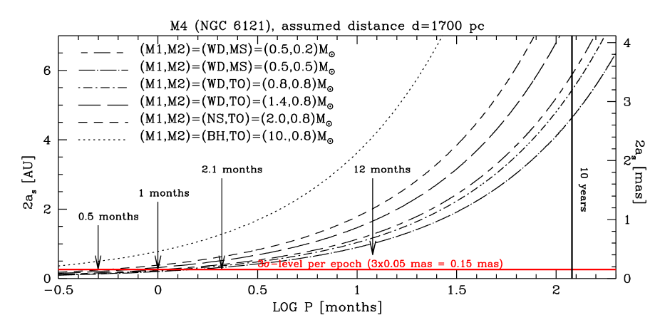
Figure 1: The relation between twice the semi-major axis 2$a_{\rm s}$ for the barycentric orbit of the luminous companion (because that is the maximum size of the total range of motion for a circular orbit that we can measure) and period (P) for binary stars of different masses. Our observing strategy should detect binaries with a minimum period of $\sim$1 month. The horizontal red line sets our limit, due to the resolution of the telescope and the precision of our method (3$\sigma$ $\simeq$0.15 mas, i.e., $a_{\rm s}$ $\sim$0.1 AU for a distance of 1700 pc), while the vertical line to the right sets the longest detectable period ($\sim$10 years) making use of the existing HST archival material.

3 The target

M 4 is our target of choice for several reasons: (1) as explained above, we expect to find a high concentration of binaries; (2) the cluster core is large and open, and we expect most of the massive binaries to have settled there, due to mass segregation; (3) M 4 is nearby, which allows study of binaries below the turn-off (i.e., more stars); (4) the closest GC is the place where the angular wobbles will be the largest. The expectation that a relatively large fraction of stars in the core of M 4 are in binaries is confirmed by the work by Milone et al. (2012a), where, using a color-magnitude diagram (CMD) for the inner 50, it was found that about 15% of the proper-motion members are above and to the red of the main sequence (MS). These must be MS+MS binaries. There should also be a population of binaries with a MS star and a massive, evolved companion [white dwarf (WD), neutron star (NS), possibly stellar-mass black hole (BH)] that cannot be detected photometrically.

Binary systems with massive remnant components must exist, simply from normal stellar evolution. Furthermore, simulations show that MS+MS binaries should tend to exchange low-mass MS companions for more massive ones, including massive WD and NS. A few heavy binaries in M 4 have indeed been revealed through their X-ray emission (Bassa et al. 2004), but the vast majority remain undetected. [Note also, that M 4 certainly hosts a pulsar, in a triple system with a WD and a planetary-mass companion, at $\sim$1 core radius $(r_{\rm c})$ (Sigurdsson et al. 2003)]. Our study is thus important for constraining not only the fraction of binaries and their properties, but also the amount of unseen mass in GCs (including the raw ingredients for the production of binaries with compact objects).

4 Expected properties of the binaries

Binaries evolve both dynamically and through their own internal evolution. We expect that the softest primordial binaries (semi-major axis, $a$ $>$ 2 AU) have almost all been destroyed. According to our current best model (Heggie & Giersz, 2008) the distribution of the semi-major axes for the present-day binaries is expected to have a median value of $a\sim$0.3 AU, with the bulk of the binaries having $a$ between 0.05 and 1.2 AU. If we want to detect binaries we need to be sensitive to the wobbles of such systems.

Our models also give the period, luminosity and spatial distribution of the binaries, and are consistent with the available information on photometric binaries and radial velocity binaries (in the outskirts). The models also include exchange interactions (Hills 1976), the main route by which degenerate binaries form. However the cross sections which were used for these processes are approximate, and so we also give the following more model-independent argument to estimate the number of heavy binaries.

To obtain an estimate of the expected number of detectable binaries, we argue as follows (bearing in mind that the aim of this project is to provide the basic data on which such estimates depend!). In the core of the Monte Carlo model there are $\sim$1800 white dwarfs (41% of all objects in the core, in agreement with the observations from GO-10146, see Bedin et al. 2009). Of these, $\sim$1200 have masses above the mass of stars at the MS turn-off ($\sim$0.8$M_{\odot}$). The model also predicts that at the present day there should be up to 1200 neutron stars within the core (depending on the retention fraction). It has been estimated (Ivanova et al. 2008) that of order 50% of NS stars in the core would form binaries by exchange, in a GC with 100% primordial binaries. Therefore we expect that, in the core of M 4, where the binary fraction is about 10%, the number of binaries with WD or NS companions could be as much as $(1200+1200)\times 0.50\times 0.10\simeq 120$, and no less than 60 with WD companions alone. According to our model, about 50% of the binaries in the core lie less than $\sim$4 magnitudes below the turn-off, and so the expected number of such binaries with WD or NS companions should be in the range $\sim$30–60. Reassuringly, the Monte Carlo models predict even larger numbers: $\sim$100.

5 Detecting the wobble

When Wide-Field Camera 3 (WFC3) was installed on HST  during Servicing Mission 4 (SM 4), we were very excited about the astrometric potential of the Ultraviolet and Visual (UVIS) channel. With a field close to that of the Wide-Field Channel (WFC) of the Advanced Camera for Surveys (ACS), and smaller pixels (0.039775 arcsec) with less Charge Transfer Efficiency (CTE) losses (to start with), WFC3/UVIS would clearly be the instrument of choice for imaging astrometry. When the Servicing Mission Orbital Verification (SMOV) images were released, we immediately set out to apply the expertise we have gained working with the ACS detectors (Anderson & King 2004a and 2006, hereafter AK) and solved for the distortion and demonstrated its astrometric prowess (Bellini & Bedin 2009). Since SMOV, many more astrometric calibration images have been taken through many more filters, and we have recently published a distortion solution for the ten most commonly used filters that is accurate to better than 0.01 pixel (Bellini, Anderson, & Bedin 2011). The solution accounts for the camera optics, filter-specific perturbations, and a $\pm$0.03-pixel manufacturing defect. Once the distortion has been removed, we are able to recover the full astrometric capabilities of UVIS. Bellini et al. (2011) demonstrates the measurement quality for a single UVIS exposure as a function of instrumental magnitude. For stars with good S/N, we achieve a single-measurement accuracy of 0.0085 pixel, or about 0.35 milli-arcsec (mas), along each coordinate (as confirmed also by our preliminary reduction of the first epoch; see Sect. 8).

The core radius of M 4 is $r_{c}$$\sim$50^′′, and therefore the WFC3/UVIS field will cover the entire core region to detect many kinds of binary systems, with various masses and periods, with typical examples summarized in Fig. 1. The range of separations that we will be able to measure corresponds to a range of periods, depending on the component masses. The horizontal red line at $\sim$0.15 mas marks where our 3-$\sigma$ astrometric detection limit will be.

The above-mentioned measurement precision in a single image (of $\sim$0.35 mas) for each star can be improved by taking many independent exposures at a variety of dithered positions within each epoch, and by adopting a local-transformation approach (Bedin et al. 2003; 2006; Anderson et al. 2006; Milone et al. 2006; Anderson & van der Marel 2010). The astrometric errors at each epoch scale as $\sim 1/\sqrt{N}$, where $N$ is the number of images on which the star is measured. The dithering and the differential-astrometric approaches allow us to mitigate any small errors in the solution for the distortion, which is surely present in images, following the procedures we have already applied to the other cameras (WFPC2, HRC and WFC: AK03a, AK04b, AK06). With $\sim$50 observations of each star per epoch, our ultimate 1-$\sigma$ precision can reach $\sim$0.05 mas (i.e. $\sim$1.2 milli-pixel).

To put this precision into context, let us consider a massive binary made of a NS (of 2 $M_{\odot}$) and a MS star (of 0.6 $M_{\odot}$) with period of $\sim$15 days. The orbit of the luminous component, the MS star (the secondary), around the center of mass of the pair, would have a semi-major axis ($a_{\rm s}$) of $\sim$0.13 AU. At the distance of M 4 ($\sim$1.7 kpc, Peterson et al. 1995) this implies a semiamplitude of the wobble of $\sim$0.075 mas. We note, in fact, that over its orbit such a star will show a total range of up to twice the barycentric semi-major axis, bringing its total excursion to 2$\times$0.075 mas = 0.15 mas, our 3-$\sigma$ detection limit. All the binaries above the red line in Fig. 1 can be discovered by our survey. As the period increases, the wobble amplitude increases, making the binary easier to detect. Data of our large program GO-12911 will be sensitive to binaries with periods up to $\sim$1-year. Although we expect only about 25% of binaries to have periods larger than $\sim$1 year, by including observations from the archive taken 4, 6, 10, and 15 years before Cycle-20, we could explore much longer periods (see Fig. 2). The lower precision of some of the archival epochs might be compensated for by the larger wobble of the longer periods.

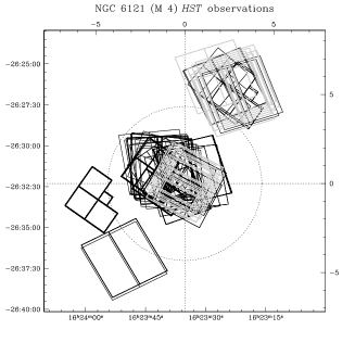
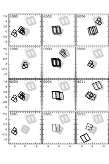
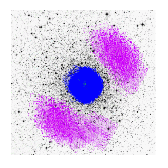
Figure 2: (From Left to Right): The first panel shows all the existing HST observations available in the M 4-field (as October 2012). The $\alpha$ and $\delta$ (J2000.0) are indicated on bottom and left axes, while top and right axes give the angular distance in arcmin from the assumed center of M 4. Dotted lines mark the center of the cluster, and the 5 arcmin angular distance. Data from the first visit of GO-12911 are indicated in grey. On the right of this panel, for reference, are shown on the same scale the footprints of the different detectors. The second panel shows in a 3$\times$4 array the archival material subdivided per year (labeled on the top-left of each box). The last panel shows, overlaid to a DSS image of M 4, the precise locations of all the planned individual images for GO-12911 (WFC3/UVIS in blue, ACS/WFC parallels in magenta, from the HST’s Astronomer’s Proposal Tool ).

Measuring the wobble of a star implies also solving for the motion of the binary system with respect to a members-rest-frame. Solving for the members-rest-frame and for the individual motions of the binary system luminous components is an iterative process.

From archival images, and as later confirmed by our first epoch, we know that there are $\sim$2000 MS stars for which we can measure high-precision astrometric positions. Figure 1 shows that the detectable binaries will have periods longer than 1 month, and our model shows that over 50% of the bright binaries in the core should have periods at least as large. Combining this with the expected number of degenerate binaries in the core, we therefore expect the survey to allow us to discover $\sim$15-30 such binaries ($\sim$30-60$\times$0.50). Our search will yield estimates of both the period and semi-major axis, and we can therefore estimate the total mass in the system. Knowing the luminosity of the MS star we can estimate its mass, then get the mass ratio $q$, and so the mass of the dark companion. The numbers and properties of these binaries are the goal of this project.

Note that GAIA will not be able to accomplish the goals of this project because of crowding, neither will JWST or ground-based AO/MCAO systems, because they operate in the near-IR where the halos of the bright red giants will interfere with the measurement of our target upper main-sequence stars.

6 Observing strategy

In planning the observing strategy, we had three main priorities:

• we wanted to maximize the number of stars in the core of M 4 with suitable S/N;

• we wanted to obtain images with the sharpest PSFs and the best possible sampling and stability;

• we wanted to maximize the number of independent exposures.

6.1 Choice of the camera

To maximize the number of stars we need to use a detector that covers the entire core of M 4 ($r_{\rm c}$$\sim$$50^{\prime\prime}$). This restricts our choice to either ACS/WFC or WFC3/UVIS in full-frame mode, as subarray-mode (which would have a better duty-cycle) is not a suitable option. We also need to suppress the light from red giants in the core of the cluster so that their wide PSF halos will not contaminate the measurement of the other stars. This can be done by using a blue filter (see next section). The choice was to use WFC3/UVIS, which has a better pixel sampling than ACS/WFC, is optimized for blue light, and has the additional advantages explained below.

6.2 Choice of filter

WFC3/UVIS (like ACS/WFC) has an optimal exposure-time of $\sim$350 s which minimizes the overhead and maximizes the duty-cycle. At the same time, to reduce our systematic and random errors (see discussions in Sect. 6.5 and 6.6) we need the largest possible number of independent exposures. For these reasons we would take as many images at the minimum-optimal length as possible ($\geq$350 s).

Just above the sub-giant branch (SGB) is where the LF takes a sharp upturn, and so using a filter that saturates just above this limit yields the largest number of stars within 4 magnitudes of saturation, where we have optimal S/N. Among the broad-band filters, with these kinds of exposure-times, F390W is the only one that saturates stars just brighter than the SGB, and for this reason, this filter was initially selected at the phase I stage of the proposal.

However, at the phase II stage —thanks also to archival and proprietary material that just became available— we realized that the PSFs in filter F390W (and in all filters bluer than $\sim$400nm) were not good. Not only did the positions turn out to be significantly color-dependent (as already demonstrated by Bellini et al. 2011), but PSFs below $\sim$400nm are also considerably wider and less stable than in redder filters.

In the end, we selected the medium-band filter F467M, since archival images showed that it saturated at the same level as F390W, but the PSF is 10% sharper, which translates directly into 10% better positions. An additional benefit of the medium-band filter is that it significantly suppresses any color-dependent effects, which are clearly seen in WFC3/UVIS’s bluer filters.

6.3 Number of exposures per epoch

In each orbit, we were able to fit 5 exposures of $\sim$390 s depth and one exposure of 20 s through F775W at the beginning of each orbit. There was no way to trade the F775W exposures for more F467W exposures, and the F775W exposures give us a handle on color issues. This strategy yields the highest number of well-exposed images of stars around the MS turn-off. Our images from the archive show that stars in this field are sufficiently isolated to be measured accurately as single stars. At the same time, there will be plenty of nearby high S/N neighbors so that we can measure each star’s position relative to a local network of its neighbors, thereby minimizing distortion errors. On average each star will be $\sim$30 pixels from any neighbor, but there will be $\sim$100 high S/N neighbors within $\sim$500 pixels (i.e. $\sim$20^′′). In Sect. 8, we show that the first epoch achieves an astromeric precision of $\sim$0.008 pixel ($\sim$0.35 mas) per coordinate. With 50 exposures in each ten-orbit epoch, this gives us a 1-$\sigma$ precision of 0.05 mas per epoch, which is our target accuracy for detecting the wobbling binaries.

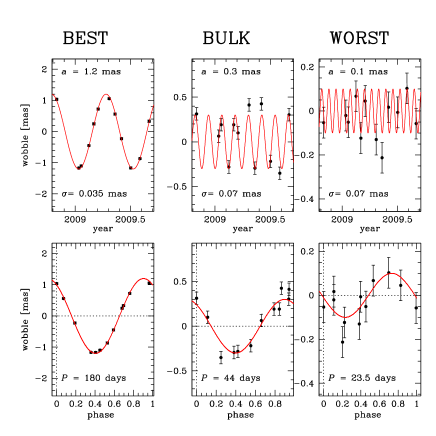
Figure 3: Examples of the expected wobbles. In three representative cases of detectable wobbles (red lines), we show how single-epoch simulated data-points (black dots) would look, assuming the barycentric semi-major axes $a$ (indicated on top of top panels) and the uncertainties $\sigma$ (on bottom of top panels). Bottom panels show the phased signals and label the periods.

6.4 Number of epochs

The problem of computing orbital elements of a binary from a set of observed positions is formally analogous to the case of orbits in the solar system, and yet in practice there is little resemblance between the methods employed. In particular measurement errors are much larger (compared to the quantities to be determined) in the binary-star case, so that an orbit needs to be based on a much larger number of observations.

There are several methods for the determination of visual binary orbits (see Heintz 1978 for a review). In our case we are dealing with pure astrometric orbits, computed (1)  from 2-D position measurements, and (2)  with no a priori information about the orbit (i.e. no RV orbit). Under these assumptions, and with our expected S/N ratio (errors of 0.05 mas on a separation of 0.20-0.50 mas, for the bulk of the binaries), simulations (such as those in Fig. 3) show that an orbit derived from twelve 2-D positions well distributed in phase over at least two binary periods should provide reliable detections. The minimum stipulation of two periods is important for confirming that our model for the tightest detected binaries ($P$$<$6 months) is predictive, and for a realistic estimation of errors. In the case of non-circular orbits it is likely that twelve measurements would determine $a$ (or at least the maximum separation) considerably better than other elements such as the eccentricity. For all the above reasons, we divided our 120 orbits into twelve 10-orbit epochs separated by a minimum of $\sim$15 days to a maximum of $\sim$3 months. This sampling should allow us to probe binaries with periods between $\sim$15 days to 6 months.

6.5 Dither pattern

For each epoch (of 50 images) we planned to use a grid of $\sim$7$\times$7 pointings with a $\sim$200-pixel step. All images will be dithered as described in AK00. The dither strategy is fundamental for the success of this program. It will be crucial: (1) to solve for the residual geometrical distortion within each epoch; (2) to solve for the effective ePSF of the undersampled detector within each epoch; (3) to have a handle on any unaccounted sources of systematic error (CTE inefficiencies, detector and optical artifacts, chromatic effects, etc…). Our choice of strategy gives the maximum dither (thus optimizing the randomization of any unremoved distortion error) while also satisfying the constraint of covering the entire core of M 4 in every exposure.

6.6 Orientations

In addition to having a large number of pointings, each epoch will have a different orientation. This will allow us to construct the most accurate possible average distortion correction. While distortion errors will be mitigated by our local transformations, it is always advantageous to start with the most accurate possible global solution. Again, this will allow us also to remove any unanticipated (and anticipated) systematic effects, while giving us the entire inner $\sim$1$.\!\!^{\prime}$8 at every visit (essentially the entire core of the cluster, see right panel of Fig. 2).

6.7 CTE mitigation

In filter F467M we have a relatively low background. Although our focus is on the bright stars, in this situation CTE might potentially introduce astrometric systematic errors at the fainter magnitudes. WFC3/UVIS is still young, but it has suffered more CTE damage than ACS/WFC had at its age. In Anderson & Bedin (2010), we designed the pixel-based correction for CTE in ACS/WFC images. The Space Telescope Science Institute is exploring the best way also to deal with CTE in UVIS data. With our observing strategy, we should have an excellent empirical handle on the impact of CTE and are confident that it will not appreciably impact our results. To further mitigate the impact of CTE inefficiencies, we have also imposed a post-flashing to all our WFC3/UVIS (see Sect. 8.2.2).

7 Previous large surveys of GCs with HST

There have been four previous HST Large Programs on globular clusters. It is interesting to compare those archival data-sets with our GO-12911 to see what this new program will add to the HST legacy.

We describe the previous programs in chronological order. GO-8267 (PI: Gilliland) used WFPC2 to observe the core of 47 Tuc. The observations were collected with a differential-photometry strategy in mind, and therefore no intentional dither is present. These data were collected in less than 10 consecutive days to be sensitive to exo-planets of Jupiter size with periods shorter than that (Gilliland et al. 2000). GO-8679 (PI: Richer) also occurred in the pre-ACS era, using WFPC2 to observe an outer field of M 4, attempting to reach the end of the white dwarf cooling sequence. Data were mildly dithered, and observations spanned about three months (Richer et al. 2002). GO-10424 (PI: Richer) and GO-11677 (PI: Richer) are similar projects to the previous one. They are both aimed at the study of the faintest stars of the clusters NGC 6397 (Richer et al. 2006) and 47 Tuc (Kalirai et al. 2012), respectively. They both studied a field in the outskirt of the clusters, and both made use of ACS/WFC. In the case of GO-10424, there are three deep images per orbit, and they were all collected in about a month. In the case of GO-11677, there are just two deep $\sim$1400 s exposures per orbit, collected in eight months. In summary, among these archival large programs, only GO-8267 observed the core of a globular cluster and focused on the same type of stars as our GO-12911, i.e., the four brightest magnitudes just below the MSTO. These facts make GO-8267 the most similar data-set to GO-12911 in the HST archive, and yet there are significant differences between the two programs. The most important difference is that GO-12911 images are collected in twelve epochs spanning one year instead of being consecutive. Second, GO-12911 images are planned to be dithered within each given epoch, which naturally worsens the differential photometric precision, but does enhance photometric accuracies, and —most importantly— it is a necessity for high accuracy astrometry. Exposure cadence ($\sim$390 s) is significantly lower in GO-12911 than in GO-8267 (160 s), but is significantly higher than in the three other Large Programs on GCs (GOs: 8679, 10424, and 11677). Interestingly, all these programs collected color information during each orbit.

GO-12911 is the first HST large program to observe the core of a globular cluster using a new generation instrument such as WFC3/UVIS and the first of the four to collect observations with large dithers.

8 First epoch

The first of the twelve epochs for GO-12911 was collected on October 9th and 10th 2012. In this section we provide the astronomical community with a report about this data-set, which should be considered as a template for what is expected from each of the remaining epochs. To this end, we illustrate the photometric and astrometric quality achieved in our preliminary reductions.

8.1 Observations

The first epoch (hereafter, epoch 01), as well as the next eleven planned, consists of ten single-orbit HST visits, during which WFC3/UVIS is the primary instrument and ACS/WFC is used in parallel. All images within a given epoch are taken with the same HST roll-angle; in the case of epoch 01, this was set to be $\textsf{ORIENT}=107^{\circ}$ (i.e., PA_V3$\simeq$286^∘).

During each orbit, HST takes 1 short exposure of 20 s in WFC3/UVIS/F775W, 5 astrometric images of $\sim$390 s in WFC3/UVIS/F467M, and a single coordinated parallel ACS/WFC exposure of 180 s, which is alternately taken through F814W and F606W (only one parallel exposure could be taken each orbit on account of buffer-dump limitations). One of the short WFC3/UVIS exposures, at the center of the dither pattern, was chosen to be collected through F467M rather than in F775W, and at the same location as the subsequent F467M long exposure. This will enable us to register our astrometry and photometry for saturated stars to positions and fluxes of the unsaturated objects. As described in Sect. 6.5, our astrometric WFC3/UVIS/F467M exposures are organized in a 7$\times$7 dither pattern, and, since in 10 orbits we can fit 50 images, we have one extra astrometric long exposure which breaks this symmetry. We chose to place this extra exposure on the background extragalactic point source described in Bedin et al. (2003) using either F467M or F775W. This way we will have a cross-check on the absolute zero-motion and an additional check on the geometric distortion in the outskirts of our studied core field.

Figure 4 shows the location of the footprints of the individual images collected during epoch 01 superposed on a Digital Sky Survey image, and Table 1 summarizes the data-set.

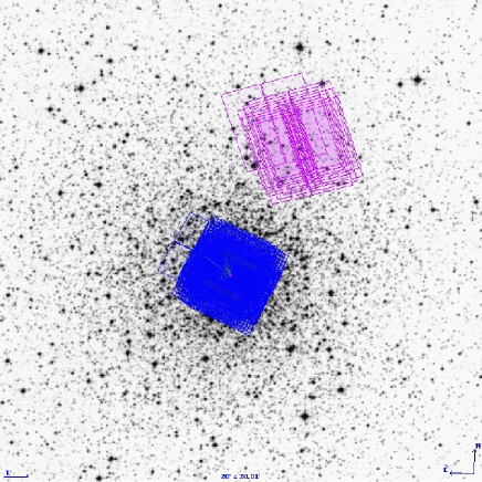
Figure 4: Layout of the observations collected during epoch 01 of M 4. The simultaneous coordinated parallel ACS/WFC images are shown in magenta, while the primary WFC3/UVIS images are shown in blue (from HST’s Astronomer’s Proposal Tool ).

To collect images in conditions as identical as possible, we plan to collect all the images, in a given epoch, within no more than three consecutive days (this was successfully done for the first 6 epochs). Tentative scheduling and roll-angles for the next visits are given in Table 2.

Table 1: Data-set summary for epoch 01 of program GO-12911. Visits: 0L,0M,0N,0O,0P,0Q,0R,0S,0T, and 0U were collected between October 9^th 2012 at UT 00:49:56 and October 10^th 2012 at UT 22:01:47.

Camera/Channel	Filter	#$\times$Exposure-time
primary observations
WFC3/UVIS	F467M	1 $\times$ 20 s
WFC3/UVIS	F467M	45 $\times$ 392 s
WFC3/UVIS	F467M	5 $\times$ 396 s
WFC3/UVIS	F775W	9 $\times$ 20 s
coordinated parallel observations
ACS/WFC	F606W	5 $\times$ 180 s
ACS/WFC	F814W	5 $\times$ 180 s

Table 2: Plans for scheduling and PA_V3 of all epochs.

Epoch ID	Date	PA_V3[∘]
01†	09-10 Oct. 2012	286
02†	18-19 Jan. 2013	92
03†	11-12 Feb. 2013	99
04†	07-08 Mar. 2013	83
05†	01-02 Apr. 2013	110
06†	24-25 Apr. 2013	124
07	18-20 May. 2013	150
08	11-13 Jun. 2013	240
09	05-07 Jul. 2013	253
10	29-31 Jul. 2013	260
11	22-24 Aug. 2013	267
12	15-17 Sep. 2013	277
† Already collected.

8.2 Data reduction and calibration

While reduction procedures for WFC3 are still being improved, the procedures for point-source astrometry and photometry in ACS/WFC images have already reached a point where any future improvement is likely to be marginal. Therefore, we will first discuss the less-preliminary reductions obtained for the coordinated parallel ACS/WFC observations, and we conclude the presentation of the new data with the more-preliminary reduction available (at this stage) for the WFC3/UVIS data.

8.2.1 ACS/WFC

All CCD detectors in the harsh radiation environment of space suffer degradation due to the impact of energetic particles, which displace silicon atoms and create defects. These defects can temporarily trap electrons during readout, resulting in Charge Transfer Efficiency losses and in trailing of the sources (because the electrons are released at a later time). These effects have a major impact on astrometric projects (Anderson & Bedin 2010) and also non-negligible effects in photometry. In this work, every single ACS/WFC image employed was treated with the pixel-based correction for imperfect CTEs developed by Anderson & Bedin (2010). The algorithm has been now improved and is now a part of the standard CALACS pipeline as _flc exposures. This correction has been shown to be effective in restoring fluxes, positions, and the shape of sources, and reducing systematic effects of imperfect CTE to less than $\sim$20% except in the case of extremely low backgrounds (Anderson & Bedin 2010, Ubeda & Anderson 2012).

Fluxes and positions of sources within ACS/WFC images were extracted with the software tools described in detail by Anderson et al. (2008). It consists of a package that analyzes all the exposures simultaneously in order to generate a single list of stars. This routine was designed to work well in both uncrowded and moderately crowded fields, and it is able to detect almost every star that can be detected by eye. It takes advantage of the many independent dithered pointings of the images and of the knowledge of the PSF to avoid including artifacts in the list. We used spatially-variable library effective PSFs documented in AK06, but the parallel fields are too sparse to allow us to improve the PSF with the software’s “perturbation” option.

The photometry was calibrated into the WFC/ACS Vega-mag system following the procedures given in Bedin et al. (2005), and using the most updated encircled energy and zero points available at the STScI’s ACS web-site. We will use for these calibrated magnitudes the symbols $m_{\rm F606W}$ and $m_{\rm F814W}$.

Finally, stars that saturate (brighter than $m_{\rm{F606W}}$ $\sim$ 18.5 and $m_{\rm{F814W}}$ $\sim$ 17.5) are treated as described in Sect. 8.1 in Anderson et al. (2008). Collecting photo-electrons along the bleeding columns allows us to measure magnitudes of saturated stars up to $\sim$3.5 mag above saturation (i.e. up to $m_{\rm{F606W}}$ $\sim$15, and $m_{\rm{F814W}}$ $\sim$ 14), with errors of only a few percent (Gilliland 2004). This treatment allows us to recover the MS TO stars also in the ACS/WFC parallel images of the outskirts of M 4.

With the transformations from the coordinates of each image into a common frame, it becomes possible to create a stacked image of the field within each epoch. The stack provides a representation of the astronomical scene that enables us to independently check the region around each source at each epoch. The stacked images are 15 000 $\times$ 15 000 super-sampled pixels (by a factor $\sim$2 relative to the image pixels, i.e. $\sim$25 mas/pixel), corresponding to $\sim$6$\times$6 arcmin².

In Fig. 5, we show on the left the depth of coverage for the ACS/WFC parallel images of epoch 01 in filter F814W, in the middle the corresponding stack image, and on the right a close-up of a representative $\sim$27$\times$27 arcsec² region. Figure 6 shows the color-magnitude diagrams obtained for stars in this ACS parallel field. The dotted lines mark the on-set of saturation. In the plots are given the instrumental colors and magnitudes (bottom and left axes), and the calibrated ones (top and right axes).

8.2.2 WFC3/UVIS

The WFC3 team has recently found (Baggett & Anderson 2012) that a small amount of post-flash ($\sim$12 e^-) can prevent a significant amount of CTE losses. In planning the observations, we examined the background in archival F467M images taken of the M 4 core for GO-12193 (PI: Lee) and found that we should expect about two electrons per pixel in a typical 350 s exposure. To get the recommended background of 10-12 e^-, we decided to add 8 e^- of post-flash to each F467M exposure. The background achieved in the first visit is about 15 e^-, a bit higher than expected, but the mitigation should still be quite good.

As mentioned in Sect. 6.7, the WFC3 team is also currently working to develop a pixel-based CTE-restoration capability similar to what has been done for ACS/WFC. This was not available at the time of the first epoch, so this preliminary analysis has been done on uncorrected images.

We measured star positions and fluxes on the WFC3/UVIS _flt images with a routine that is similar to that described in AK06 for the WFC/ACS. We used “library” PSFs that were extracted from F467M observations of $\omega$ Centauri that accounted for the static spatial variability. We also constructed a distortion solution for F467M from the same data set. (As more data become available for this field, this program will allow a definitive distortion solution and average PSF for F467M.) These positions and fluxes were corrected for distortion and used to relate each exposure to the master frame.

We then used a software program that is similar to that developed by Anderson et al. (2008) for the ACS Survey of Galactic Globular Clusters (GO-10775, Sarajedini et al. 2007) treasury project to go through the field in 120$\times$120-pixel tiles to iteratively find and measure stars simultaneously in all 50 contributing WFC3/UVIS/F467M 390 s exposures. Figure 7 shows the depth of coverage for the WFC3/UVIS observations, an image of the field, and a close-up of a representative 20$\times$20 arcsecond region. Figure 8 shows the color-magnitude diagrams obtained from this initial finding run in the WFC3/UVIS core field. The dotted lines mark the saturation level (the dashed line marks the on-set of saturation for 20 s short exposures in F467M).

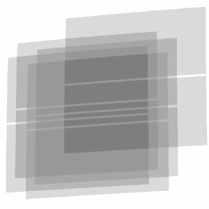
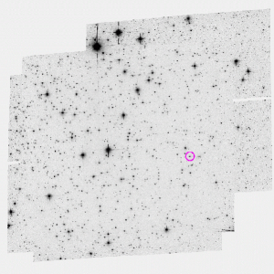
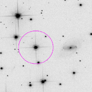
Figure 5: (Left:) depth of coverage map for the five ACS/WFC/F814W images collected within epoch 01. (Middle:) resulting stack image. (Right:) a $\sim$$27^{\prime\prime}$$\times$$27^{\prime\prime}$ zoom-in around the star marked with a circle in the previous panel. For reference, the circle has a 200-pixels radius (in the ACS/WFC stack the pixel scale is $\sim$25 mas).

Figure 6: Color-magnitude diagrams for the coordinated parallel observations with ACS/WFC using the 5 images for each filter. The distributions of dots fainter than instrumental magnitudes of $-$5 and centered at 0 in color, indicate the floor-level of white noise.

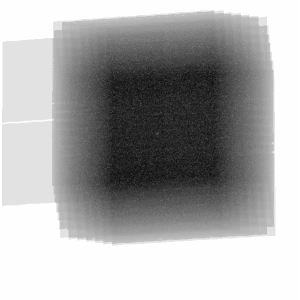
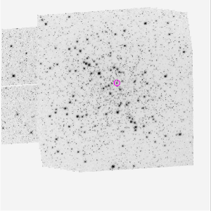
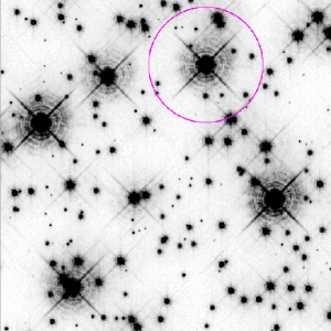
Figure 7: (Left:) depth of coverage map for the 50 WFC3/UVIS/F467M deep astrometric images of epoch 01. (Middle:) resulting stack image. (Right:) a $20^{\prime\prime}$$\times$$20^{\prime\prime}$ zoom-in at the center of M 4. For reference a circle with a 200-pixels radius is shown (WFC3/UVIS stack has a pixel scale of $\sim$20 mas). Note that diffraction spikes will have different orientations at the different epochs.

Figure 8: Color-magnitude diagrams of sources in the WFC3/UVIS field, obtained by combining the photometry from the 51 F467M images and the 9 WFC3/UVIS/F775W images. Magnitudes are instrumental, and the dotted lines indicate the on-set of saturation. Dashed line marks on-set of saturation for the 20 s short exposure in F467M.

8.3 Preliminary astrometric precision

The motivation for this program came from the finding in Bellini et al. (2011) that stars can be measured with a precision of $\sim$0.35 mas in each coordinate in a single exposure. We show below that even our preliminary reduction of the first epoch already achieves this goal.

To determine astrometric uncertainties, we measured each star in each exposure, corrected its position for distortion, then used a general 6-parameter global linear transformation to estimate its position in the reference frame. The scatter of these many estimates gives us an indication of the measurement uncertainty. The left panel of Fig. 9 shows the 1-D rms among the measured positions.

We computed the 68th percentile of the distribution of these rms in every half-magnitude bin (red filled circles). A solid line (in red) through these points highlights the behavior of the rms as a function of the magnitude (i.e. as a function of the S/N). This shows that even with a global transformation the positional errors for the typical star just below saturation is on the order of $\sim$0.01 WFC3/UVIS pixels (i.e. $\sim$0.39 mas). Two dotted lines mark the 0.008 and 0.006 pixel level (i.e. the 0.24 and 0.32 mas precision level).

We find that these errors are further reduced when we use local transformations from each frame into the reference frame. Local transformations absorb most of the residuals in the geometric distortion due to the imperfection on the PSF models, detector features, particular status of the focus, and of the optical alignment in general (see Bedin et al. 2003 or Anderson et al. 2006 for more details). In computing local transformations we employed the 101 stars closest to the target, within 500 WFC3/UVIS pixels, with an instrumental magnitude brighter than $-10$. The right panel of Fig. 9 shows the 1-D precision for this local transformation approach. This plot demonstrates that a precision of $\sim$0.25 mas can be reached for the brightest unsaturated objects (i.e., almost 30% better than our nominal requirement).

We want to emphasize that these results are still preliminary for the following reasons:

1. in this data reduction, no pixel-based mitigation of CTE problems was performed, neither in $x$ nor in $y$ (serial and parallel readings);

2. the PSFs were taken from a library; they are spatially variable but not tailored to the particular focus-state of the telescope during the given individual exposure;

3. the geometric distortion correction for filter F467M is still crude; in the end we will expect to have an almost perfect characterization of the geometric distortion in this filter, significantly better than what was done for the 10 filters in Bellini et al. (2011), thanks to the huge —unprecedented— amount of data available.

We also plan to attempt a modeling of the perturbation to be applied to both the average PSFs and the average geometric distortion correction, as a function of the HST position telemetry, angle between Sun and telescope tube, temperature, etc, using de-correlating techniques. Nevertheless, we note that, in spite of the crudeness with which it was derived, the above-described 1-D precision of $\sim$0.3 mas, for a well-exposed star, already meets our project requirements.

It will be extremely easy to separate background stars from cluster stars by means of the proper motions. The field-cluster separation is hundreds of times larger than the astrometric wobbles of binaries we propose to measure here. Field-objects mainly belong to the outskirts of the Galactic Bulge, which is in the background of M 4. To demonstrate this PM separation, we downloaded from HST ’s archive images collected under program GO-10775 (PI: Sarajedini) on May 3rd, 2006 (Sarajedini et al. 2007), and use them as a previous epoch. We reduced _flc ACS/WFC images in filters F606W and F814W, 4 per filter of 25-30 s, and extracted fluxes and positions.

In Figure 10, the top panels show the proper-motion diagrams for the common objects to the two data sets. In the bottom, the corresponding calibrated color-magnitude diagrams are shown. From left to right, the plots refer to the entire sample, the sample with cluster motion (arbitrarily defined as proper motions smaller than 3.5 mas yr^-1), and the objects with field motions, i.e. with proper motions larger than that.

Figure 11 shows a three-color stacked image of the central field. Since the cluster stars were used as the basis for the transformations, they have no motion in this frame. But field objects appear as rainbow trails, with an offset between their green and red+blue light.

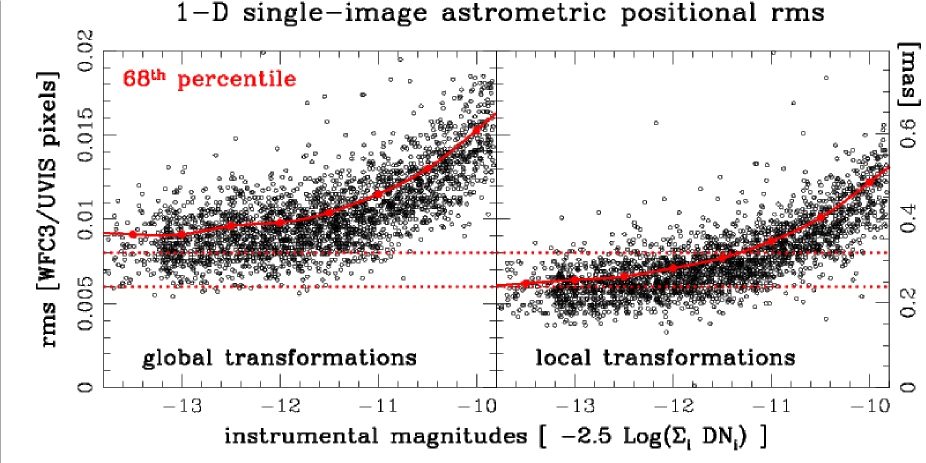
Figure 9: (Left): Each small black circle is the root mean square (rms) of the $x$-positions of unsaturated stars measured in at least 38 (and up to 50) individual WFC3/UVIS/F467M images once transformed —with the most general linear global transformation— into the adopted reference frame, and plotted as function of the instrumental magnitude. Every half-magnitude bin, a red dot indicates the positions of the 68^th percentiles of the distribution, $\sigma$. A solid line (in red) connect these points. For reference two horizontal and dotted lines (also in red) mark the 0.006 and 0.008 WFC3/UVIS-pixel levels (i.e. 0.24 mas and 0.32 mas). (Right): Same plot for same stars, but this time using local transformations. The positioning random error for the brightest stars is now $\sim$0.25 mas. The reduction is still preliminary (see text) but 50 dithered images with this precision should be able to lower the error on the mean $\overline{\sigma}$ to below the required detection limits of $\overline{\sigma}\simeq 50\mu$as. Units of WFC3/UVIS pixels are given on the left, while the ordinate on the right reports units of milli-arcsec (mas).

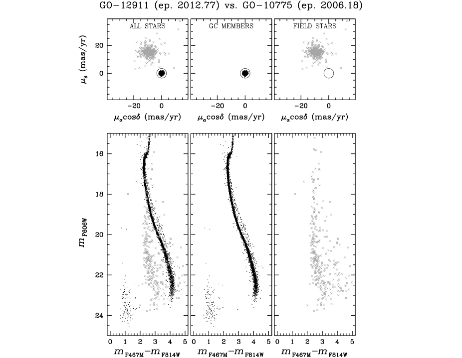
Figure 10: Primary field in the core of M 4: (Top): Proper-motion diagrams (in mas yr^-1 units) obtained comparing displacements between average positions measured in epoch 01 and those measured in the archival ACS/WFC images collected in 2006 under program GO-10775. (Bottom): Corresponding calibrated CMDs for objects in the above proper-motion diagrams. (Left): The entire sample of all common objects to the two data-sets. (Middle): Objects assumed to be members of the GC, i.e. with proper motions smaller than 3.5 mas yr^-1 (criterion highlighted by circles in the top panels). (Right): Objects with proper motions greater than 3.5 mas yr^-1, and considered field objects. In all panels, members are indicated with dots and field objects with crosses.

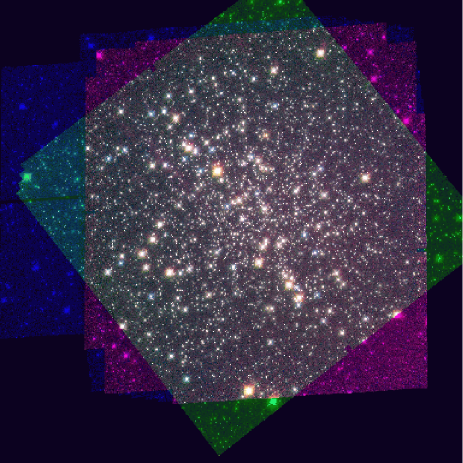
Figure 11: (Left): Three-color image of the core of M 4, where for the blue- and red-channels we used the WFC3/UVIS/F467M and F775W GO-12911 images, and for the green-channel we used ACS/WFC/F606W images from GO-10775 collected $\sim$6 years earlier. (Right): Close-up of a region in the same image of $\sim$$13^{\prime\prime}$$\times$$13^{\prime\prime}$. Note that, as the transformation is computed with respect to cluster members, which define the zero of the motion, the field objects appear as trailed rainbows.

8.4 Preliminary photometric precision

As noted before, the observing strategy of GO-12911 is not meant to be optimal for differential photometry, as the adopted large dithers leave our photometry at the mercy of the accuracies of the flat-fielding (both L-flats and P-flats), and precise photometry is also affected by the locations of artifacts and manufacturing features, which vary their positions with the different dithers and orientations. Nevertheless, the photometric accuracy is still quite good, even for our preliminary reduction. Figure 12 is the photometric analog of Fig. 9 for positions, where instead of 1-D rms of $x$-positions we show the rms in magnitude. Indeed, it is possible to apply local corrections also to fluxes to remove systematic trends. We used the same network of local stars as in the previous figure. Figure 12 demonstrates that for the brightest stars we are able to achieve a photometric accuracy of $\sim$5 milli-magnitudes, i.e., still significantly worse than shot-noise ($\sim$3 milli-mag). Using techniques similar to those presented in Nascimbeni et al. (2012), we expect our final photometry to further approach the theoretical limit.

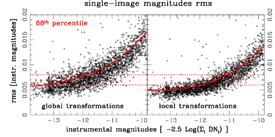
Figure 12: As in Fig. 9 but for magnitudes instead of $x$-positions. Ordinates axes are all in units of magnitudes, and the two dotted horizontal lines mark the level of a 6 and 8 milli-mag precision.

9 Planned upcoming works

The final data-set of program GO-12911 will consist of 840 HST images (720 WFC3/UVIS primary and 120 ACS/WFC parallels) and will have many unique characteristics that were not available in any of the previous HST programs (see Sect.7). The target and cadence of this data set enable a large number of studies, and our team has identified our top priorities. Our focus will be on: a search for binaries with massive and dark companions (the main project); a search for exo-planets; a search for stellar variability and X-ray$\setminus$optical counterparts; the measurement of the cluster absolute proper motion and of the cluster parallax; the measurement of internal motions of stars in the cluster core; the search for an intermediate-mass black hole; and the study of the multiple stellar populations in the cluster. All of these sub-projects together will produce improved constraints for our dynamical modelling of the present-day M 4 and of its dynamical evolution history (Sect. 9.13). This unique data-set will also allow us to perform a number of technical studies and instrument calibrations, which we will make publicly available (Sect. 9.14). One of the major outcomes of this project will be a catalog of sources in the center of M 4 of great richness (Sect. 9.15).

In the following sections, we describe in more detail the particular sub-projects (which we also list with the time-frame in Table 3) that our team will be focusing on.

9.1 Binaries with massive dark companions

The fundamental goal of the project is to detect the fraction of binaries with a massive and dark component, through the astrometric wobbles induced on their luminous companions, within the GC M 4. The motivation for this investigation and the currently-expected properties of these binaries were given in Sections 2 to 4, while Sections 5 and 6 described how this goal has driven our observing strategy. The detected wobbles will provide periods and semi-major axes, which in turn can provide the absolute masses, and mass-ratios $q$ of these binaries. These will be used to constrain our dynamical model (Sect. 9.13) and infer fundamental properties of the primordial binaries, a basic ingredient for tracing the dynamical evolution of clusters. In this section we briefly describe the analyses of reduced data and publication strategy for this task.

In order to analyze our data set, we need to find the best average (spatially variable) PSF and the best average distortion solution (these are related to each other). This will allow us to find the best position and proper motion for each star. With that, we can predict the position of each star in each exposure. To measure a given star, we will first find its nearest bright isolated neighbors within $\sim$500 pixels (as motivated in Sect. 6.3 and shown in Sect. 8.3 for epoch 01). We will use the predicted positions and fluxes for these neighbors to extract a local PSF from them (actually, a local perturbation on the global PSF for that location). Then, we will use this local PSF to measure an empirical position for the target star. This will give us a position that can be directly compared against the predicted position (based on the linear proper motions). These residuals can be used to either improve the average positions/motions or to look for wobble.

We will necessarily have to wait for all epochs to be collected. The binary-system barycentric motions need to be solved for and disentangled from their wobbles and residuals using a periodogram-type analysis to detect significant and periodic deviations from the linear motions. Most of the effort will go into identifying sources of systematic errors and in correcting for them. Artificial-star simulations will be an important aspect of this effort.

Some photometric modulation of the light curve, phased with the astrometric wobbling signature, might also be present as a result of ellipsoidal variations and synchronization of the spin and orbital motion induced by the dark companion on the luminous member of the binary system. These effects would provide us with additional confirmation of the detected wobbles.

9.2 Search for variable stars

Our survey will generate $\sim$600 high-quality F467M images of the core of M 4, split into 12 epochs (each one covering $\sim$15 nearly-consecutive hours) and spanning a year. We can also take advantage of some color information extracted from the F775W images taken at the beginning of each orbit ($\sim$120 frames overall). We will search for variability of every point-like source robustly detected in a minimum number of frames. The photometric signal of a variable star can span an extremely large range of amplitudes, shapes and periodicities according to its class (eclipsing, pulsation, rotation, cataclysmic variable, etc…). We will tune different software tools in order to maximize the detection rate of each variable class, including weighted and multi-harmonic periodograms (Schwarzenberg-Czerny 1999; Zechmeister & Kurster 2009).

Eclipsing binaries (EBs) are expected to dominate the sample of photometrically detected variables among cluster members. This is a fourth, complementary, approach to finding binaries in M 4, after detection through radial velocity (RV) variations, photometric offset in the CMD (high $q$ MS+MS binaries), and astrometric wobbles. The average photometric precision ($\sigma\lesssim 5$ mmag) on the brighter part of our sample and the time-sampling, are such that we expect a non-negligible efficiency up to long orbital periods ($P\lesssim 15$ days). M 4 is intrinsically much richer in binaries than other well-studied GCs such as NGC 6397 and 47 Tuc (Milone et al. 2012a). M 4 is also dynamically old and we expect most binaries to have sunk into its central region. By rescaling the yield of EBs estimated by Nascimbeni et al. (2012) in NGC 6397, we expect a few tens of detections from our data set. Some of them will be SB2 detached systems bright enough to be suitable for a ground-based RV follow-up on 8-10 m class telescopes. For these, an accurate estimate of the masses and radii of the binary components will be feasible, as further explained in Sect. 9.9.

Single rotational variables, whose periodicity is dominated by the intrinsic rotational period of the star are another possible outcome of this search. Gyrochronology tells us that stars in old systems such as GCs should have stars with rotational periods of several months, and photometric amplitudes of a few mmags (Chaname & Ramirez 2012). We will be in the position to measure some of these periods and, possibly, for the first time to define a gyrochronological sequence for a GC.

We will also search for variability on the ACS/WFC parallel fields. A large fraction of these fields (over 50%) will be repeated during our survey (from 5 to $\sim$30 times per filter), allowing us to detect periodic variables in a much less crowded region of the outskirts of M 4 (see right panel in Fig. 2). This investigation will provide us with important information on the radial distribution of the different classes of variables. However, we expect few binaries there, as by examining a 120 orbit WFPC2 integration in the outskirts of M 4, Ferdman et al. (2004) found a variability fraction of just 0.05% for a deep field located at six core radii from the cluster center.

9.3 Search for transiting exo-planets

Planets in star clusters offer a unique opportunity to probe how the chemical and dynamical environment affects the formation and evolution of planets. To date, searches for planetary transits carried out in GCs have yielded no confirmed detections (see Zhou et al. 2012 for a review). In the two most significant cases (47 Tuc and $\omega$ Cen) these results imply a lower occurrence of giant planets compared with field stars in the solar neighbourhood (Gilliland et al. 2000; Weldrake et al. 2008). Still, it is not clear how and why the cluster chemical or dynamical environment inhibits planetary formation or survival, and whether smaller planets such as Neptunians are affected in the same way as gaseous giants.

Some of us previously performed a search for transiting planets and variables in a deep stellar field of NGC 6397 imaged by HST-ACS/WFC over 126 orbits (Nascimbeni et al. 2012). The light curves were corrected for systematic trends and inspected with several tools, including a box-fitting least-square algorithm (BLS, Kovács et al. 2002) to perform transit-finding in the BLS periodogram. These data were not optimized for a transit search, and no significant conclusion was drawn on the planet occurrence in NGC 6397 due to poor statistics and temporal sampling. However, we did demonstrate that most NGC 6397 MS members (98%) are photometrically very stable, as they show an intrinsic jitter below $\sim$2 mmag on the time scale of a typical transit (few hours), and we expect the intrinsic jitter to be of the same order of magnitude for M 4.

We have run “inject-and-recover” simulations based on synthetic light curves that have the same noise level and sampling times as the 12-epoch photometric series expected at the end of the program. The observing strategy is still far from optimal for transit searches, since this program is designed for other purposes. Nevertheless, the advantages of GO-12911 data over those used by Nascimbeni et al. (2012) are evident (faster cadence, larger temporal coverage, larger number of imaged cluster members). We will achieve a $\sim 40\%$ efficiency in detecting transiting “hot Jupiter” planets with orbital periods shorter than 4 days. Chances to detect a Neptune-size planet are much lower (but not negligible: $\lesssim 5\%$ at $P<3$ days) due to their shallower transits. On the other hand, Neptunian planets are expected to be much more common than gaseous giants, and –even more importantly– their occurrence does not seem to decrease at lower metallicities (Howard et al. 2012; Mayor et al. 2011). This will compensate the final expected yield of planets, implying that in principle detections of Neptunian planets around the MS stars of a GC could be feasible here for the first time. At the very least, we will be able to set an upper limit on planet frequency in M 4. We end this section noting that at least one planetary-mass object is already known to exist among member stars of M 4 (Sigurdsson et al. 2003).

9.4 Absolute proper motions and annual parallax

To achieve the main goal of our project (i.e., to detect the wobbling binaries) we will refer our proper-motion measurements to M 4 member stars, which are all at the same distance, so that we will not be affected by either the absolute proper motion of the cluster or its annual parallax. At a distance of 1.7 kpc, the annual parallax of M 4 is anything but negligible: $\sim$0.6 mas (i.e., 12 times larger than our target accuracy for individual high S/N stars in a given epoch). So, in addition to the reflex of the absolute proper motion of the cluster, we expect to see the few background stars, galaxies, and QSOs (such as the one used by Bedin et al. 2003) to wobble by that much with respect to the average of M 4’s stars.

Our epochs will map the annual parallax phases almost homogeneously, and in combination with archival material (and also in combination with our parallel fields), we will be able to derive one of the most direct, accurate and model-independent estimates of the geometric distance of M 4, through the estimate of its absolute annual parallax. We will likely achieve an uncertainty below 5% on the distance, the exact value depending on the number of available extra-galactic sources.

Most of the field objects are background stars belonging mainly to the outskirts of the Galactic Bulge. It should be straightforward to determine the relative parallax of M 4’s stars (at $\sim$1.7 kpc), with respect to the bulk of the Bulge’ stars in the field (at $\sim$8 kpc, see Bedin et al. 2003). For the few stars in the foreground of M 4 in our main field, we will derive exquisite relative annual parallaxes with respect to M 4.

9.5 Multiple stellar populations within M 4

Spectroscopic studies of bright RGB stars in M 4, have shown significant star-to-star light-element abundance variations (Norris 1981; Gratton et al. 1986; Brown & Wallerstein 1992; Drake et al. 1992; Smith et al. 2005), with sodium-oxygen and magnesium-aluminum correlations (Ivans et al. 1999; Marino et al. 2008; Villanova & Geisler 2011). High-resolution VLT/UVES spectra for about one hundred RGB stars revealed two groups of stars in the Na versus O plane. Na-rich/O-poor, and Na-poor/O-rich stars populate two different sequences along the RGB in the $U$ versus $U-B$ CMD. Na-poor stars populate a spread sequence on the blue side of the RGB, while Na-rich stars define a narrower red sequence (Marino et al. 2008). M 4 also features a bimodal HB, which is well populated both on the red and the blue side of the RR-Lyrae gap. As suggested by Norris (1981) and Smith & Norris (1993), HB stars exhibit a bimodal Na and O distribution similar to what has been found for RGB stars, with red-HB stars having chemical composition similar to halo field stars and blue-HB stars being oxygen depleted and sodium enhanced (Marino et al. 2011).

While the RGB and HB have been widely investigated from ground-based photometry and spectroscopy, there are no high-precision photometric studies on multiple stellar populations among MS and SGB stars. Recent papers demonstrated that any two-color diagram made with ultraviolet and visual filters are powerful tools to disentangle multiple populations and to estimate their helium content (Milone et al. 2012b,c). The combination of the exquisite visual photometry expected from our GO-12911 data with photometry in WFC3/UVIS/F275W from GO-12311 (PI: Piotto) is expected to provide CMDs with accuracy of a few milli-magnitudes, therefore allowing us to disentangle the two stellar components also along the MS of M 4.

If we will be able to photometrically distinguish these two stellar groups among un-evolved stars, not only will we be able to infer the abundances of CNO and He (as already done for other GCs by Milone et al. 2012b,c), but thanks to our proper motion precision we should also be able to highlight potential differences in the ensemble (projected tangential) kinematics of the two stellar groups down to velocities of a few 100 m s^-1. These differences in the kinematics, combined with the radial distribution, would provide important constraints on the formation and evolution of the multiple stellar populations (D’Ercole et al. 2008; 2011).

9.6 Intermediate-mass central black hole and internal dynamics

Our investigation will yield accurate relative proper motions for a large number of stars in the central region of M 4. These internal motions of M 4 will allow us to search for a possible rise ($v\propto r^{-0.5}$) in the central velocity dispersion due to the presence of an intermediate-mass central black hole (IMBH). Assuming a mass of $M_{\rm BH}$$=$$10^{3}M_{\odot}$ (Kormendy & Richstone 1995) and a velocity dispersion of $\sigma_{0}$$\sim$3.5 km/s (Peterson et al. 1995), the black hole would have a sphere of influence of $r_{\rm BH}=GM_{\rm BH}/(3\sigma_{0}^{2})\simeq 24,000$ AU, corresponding —at the distance of M 4— to 142, or $\sim$350 WFC3/UVIS pixels. Moreover, any cluster star particularly close to the central black hole would have an extremely high velocity (Fig. 13), which we will be able to measure trivially (there are about 100 stars within this radius). This would be a tremendously exciting finding.

It is also interesting to consider that if —by chance— any background Bulge star is projected within $\sim 0^{\,\prime\prime}\!\!.\,5$ of the location of the cluster center we might be able to put even better constraints on the presence of an IMBH based on lensing constraints.

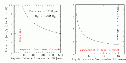
Figure 13: Expected size of the proper motion of a MS star around a central BH of 1000 $M_{\odot}$, as a function of the distance from the BH. The two panels show the expected motions at different scales.

9.7 Spectroscopic follow-ups

For stars brighter than $V$$\sim$20-21, a spectroscopic follow up is feasible with 8-10 m-class telescopes (VLT, SALT, Gemini, Keck, etc…). This offers the possibility of obtaining complementary information which could put strong constraints on many of our investigations. In the following we list some of the applications which would benefit the most from spectroscopic follow-up.

• Detecting the astrometric wobble of the bright component around a dark companion would provide information on the projected orbit of the binary system on the plane of the sky. However, obtaining the RV-curves with a precision of few km s^-1 would not only confirm the wobble detection (being phased with the astrometric signature) but would also provide the third component of the motion, and it would enable us to firmly constrain most of the orbital parameters of the system. These spectroscopic follow-ups should be possible for target stars brighter than $V\sim 20$-21, with no neighbor stars within 0.6^′′ brighter than $\Delta V=V_{\rm neighbor}-V_{\rm target}\simeq 2.5$.

• If any detached eclipsing binaries (dEBs) are discovered within our survey, detailed RV-curve follow-up would allow us to measure masses, radii and distances of the components (see Sect. 9.9 for a more extensive discussion).

• Additional RVs to those collected in Sommariva et al. (2009) for stars in M 4 would enable us not only to obtain the line-of-sight velocity of the stars in the outskirts of the cluster (which are used to constrain our dynamical model, Sect. 9.13) but also to better constrain the binary fraction and their orbital parameters through RV variations.

• If our survey happens to detect an exo-planet candidate transiting a member MS host star, a detailed RV follow-up study could exclude obvious false alarms. This should be possible for stars brighter than $V\sim 18$.

• As mentioned in Sect. 9.5, M 4 hosts at least two stellar populations. Our sub-milli-magnitude photometry and precise kinematics are expected to clearly disentangle these components even among stars in the unevolved phases. We intend to isolate a significant sample of MS stars and collect high-resolution spectra to study in detail the chemical differences between the two components down to $V$$\sim$20, as done for $\omega$ Cen (Piotto et al. 2005) and NGC 2808 (Bragaglia et al. 2010).

9.8 Photometric binaries

The fraction of MS+MS binaries with a relatively high mass-ratio (i.e. made of two luminous components) is also an important ingredient for the modelling of M 4. We plan to refine the estimate of the fraction of MS+MS binaries, and their mass-ratio distribution using our high precision CMDs and applying the methods and procedures described in great detail in Milone et al. (2012a).

On the basis of our wider color baseline, F467M vs. F775W, two times wider than the F606W vs. F814W used in Milone et al. (2012a), and of the anticipated photometric precision, we expect to be able to estimate the photometric binary distribution down to lower mass-ratios ($q$) than was possible with previous data sets (which were limited to $q$$>$0.5). Our dithered images in WFC3/UVIS/F467M and in F775W guarantee sub-milli-magnitude precision in the study of the MSs of M 4.

Differential reddening and the presence of multiple stellar populations within M 4 will complicate our analyses. We will follow the method described in Milone et al. (2012d) for the case of NGC 2808, a cluster with three MSs and comparable reddening to M 4.

9.9 Information from accurate masses and radii of dEBs

Despite a number of studies that have presented well calibrated photometry and high-precision CMDs of Galactic GCs, the ages and helium abundances of their stellar populations remain very uncertain. This is because of correlated uncertainties in distance, reddening, color-temperature transformations and metallicity, further complicated by the interplay between evolutionary times and the unknown helium contents. Detached eclipsing binaries offer the possibility of determining precise and accurate masses and radii for the system components, nearly independent of model assumptions (Andersen 1991; Torres et al. 2010). If one or both of the binary components are close to the MS TO, it is possible to put tight constraints on the age of the system by comparing the position of the primary and secondary in a mass-radius (${\mathcal{M}}$-${\mathcal{R}}$) diagram to theoretical predictions. For stellar clusters, such an analysis has significant advantages: the determination of the masses and radii is independent of the usual CMD uncertainties such as distance and reddening (the latter being particularly complex in the case of M 4, see Hendricks et al. 2012), and one avoids the difficult process of transforming the effective temperatures and luminosities of the models to observed colors and magnitudes.

Thus, determining cluster ages in the ${\mathcal{M}}$-${\mathcal{R}}$ diagram allows a direct comparison between observations and theory. We intend to follow-up with 8-10 m class telescopes the dEBs of interest that our HST survey might discover, allowing us to use similar methods to those of Brogaard et al. (2011, 2012): we will measure masses and radii with accuracies of $\sim$1% for the dEBs along with spectroscopic $T_{\rm eff}$ and [Fe/H] values from spectra of individual components obtained by decomposition of spectra of the binary stars. This procedure will be possible for the brightest dEBs (i.e., $V$$<$20).

The derived values for the individual components of the binaries will then be used in combination with the observed CMD to tightly constrain the stellar models and the cluster parameters, including the age and the helium content, the latter at the $\sim$1% level. If a cluster hosts multiple stellar populations, characterizing at least two dEB systems for each stellar population would lead to a robust estimate of age and the He abundance for each sub-population. A difference in He directly translates into differences in stellar structure, in particular the radius, leading to a clear separation in the ${\mathcal{M}}$-${\mathcal{R}}$ plane. Importantly, it is the relative locations (not absolute) of these ${\mathcal{M}}$-${\mathcal{R}}$ sequences that reveal the effect, and, unlike a difference in age, a difference in He is visible even for stars down the MS.

The combination of geometric distances (see Sect. 9.4 and 9.11), CMDs, and $T_{\rm eff}$, radii, and masses of binary components will provide unprecedented tight constraints on stellar models of the old populations of the Milky Way.

9.10 ACS/WFC parallel fields

Together with our primary observations we will collect a single ACS/WFC image per orbit, in coordinated-parallel mode. Unfortunately, the time needed for the frame-dump buffer does not allow for the collection of more parallel images.

Located at $\sim$6^′ from the cluster center, the ACS/WFC parallels will map fields well within the cluster tidal radius ($r_{\rm t}$$\sim$30^′). The data collected by ACS/WFC will be used for a number of studies in the outskirts of the cluster. As identification of photometric MS+MS binaries does not need temporal sampling, we will also be able to measure their fractions (cfr. Sect. 9.8) in the outskirts of M 4. Although we will be able to probe only relatively large $q$ in these parallel fields, it will be possible to study the radial distribution of these binaries. Furthermore, since we will see a few of the brightest WDs along the cooling sequence we will also see WD+MS photometric binaries. In addition we shall obtain the MS mass function (as in Bedin et al. 2001), and an empirical measurement of mass segregation, which will help to tighten the constraints on our dynamical models of M 4.

ACS/WFC parallel images are significantly deeper, less crowded, and less absorbed (because of the filters) than the primary WFC3/UVIS observations, and therefore we also expect them to contain many more back-ground galaxies at relatively high S/N (see an example of a back-ground object in the right-panel of Fig. 5). These parallel images will provide absolute high-accuracy proper motions in the outskirts of M 4 (especially if coupled with archival material, see left and middle panels of Fig. 2).

Combining the absolute proper motions obtained from the primary WFC3/UVIS observations in the core, and from the parallel ACS/WFC images in the outskirts of M 4, will allow us to measure other fundamental parameters of the cluster dynamics, such as the anisotropy between radial and transverse proper motions. Anisotropy is an additional constraint on the planned new dynamical models of M 4, as described in Section 9.13.

Absolute proper motions in the outer fields will enable us to obtain the average cluster rotation projected on the plane of the sky, as done by Anderson & King (2003b, 2004b) for the case of 47 Tuc.

Figure 10 and the related text, presented in Sect. 8.3, illustrate the proper-motion separation between field and cluster objects in our M 4 core field, using the WFC3/UVIS primary observations. Here, we want to show an example of the proper motion precision possible also for objects observed in the ACS/WFC parallel fields, once combined with archival material (when available). In Fig. 14, we compare positions obtained with our ACS/WFC/F814W images collected during epoch 01 (listed in Table 1) with three images collected under program GO-12193, available from the HST archive. The latter consist of just two exposures of 200 s and 450 s in ACS/WFC/F606W and one of 400 s in ACS/WFC/F814W collected in July 9, 2011, for a time base-line of just $\sim$1.25 years. In the left panel we show a portion of the CMD presented in Fig. 6 (in instrumental magnitudes), where stars in common between GO-12911 and GO-12193 are shown in black, and those not measured in GO-12193 are shown as gray points. Saturation is indicated by dotted lines. The middle panel shows the summed-in-quadrature displacements along the two axes vs. the magnitudes. The units are in ACS/WFC pixels ($\sim$50 mas) in $\sim$1.25 years. Stars on the left of the dashed line are assumed to belong to the cluster. Adopting this selection criterion, on the right panel of Fig. 14 we show the same CMD decontaminated of most field objects, and in calibrated magnitudes.

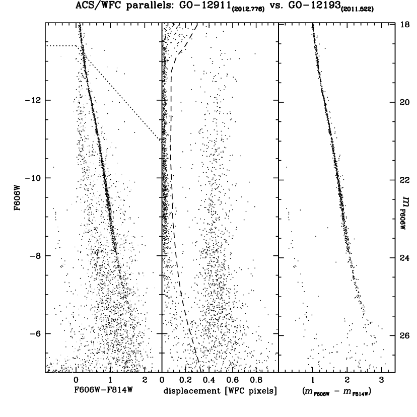
Figure 14: A parallel field in the outskirts of M 4: (Left:) a portion of the instrumental CMD shown in the left panel of Fig. 6. Stars not measured also within GO-12193, or for which it was not possible to obtain a proper motion, are indicated as grey dots. The dotted line marks the onset of saturation. (Center:) the sizes of the proper-motion displacements (in units of ACS/WFC pixel in $\sim$1.25 years) are plotted vs. the magnitudes. The dashed line marks our proper-motion cutoff criterion for membership. Stars on the left of that line are here defined as members. (Right:) shows the calibrated CMD for these member stars. The main cluster features are considerably decontaminated from field objects.

9.11 Distance to M 4

We mentioned in Sect. 9.4 our plans to determine the absolute annual parallax of M 4 in order to derive the most direct (and model independent) estimate of the distance of this GC, which is the closest one to us. However, we also plan to use three additional methods to obtain independent estimates of this important parameter of the cluster. The alternative methods are less direct, but a comparison of the derived distances with that obtained from the annual parallax offers a sanity check on the theory adopted to build the cluster dynamical model and on the adopted stellar evolutionary models. The methods are:

i) Comparison of the cluster internal dispersions of the radial velocities $(\sigma_{\rm RV})$ with the dispersion of the internal proper motions $(\sigma_{\rm 1-D\mu})$. Crudely, combining the linear dimension ($\ell$) and the angular size ($\vartheta$) of the same object (in this case $\sigma_{\rm RV}$ and $\sigma_{\rm 1-D\mu}$, respectively), provides the distance ($d\simeq\ell/\vartheta$). Unfortunately, this estimate is less straightforward than it looks (Peterson et al. 1995). First it requires an extremely careful evaluation of the error budgets (measurement uncertainties need to be subtracted in quadrature from the observed dispersions to get the true intrinsic dispersions). Second, the assumption of isotropy of the velocity distribution is not necessarily justifiable for a real cluster. This is further complicated by modulations of the dispersion by unresolved binaries, and by the fact that RVs are available mainly for bright stars in the outskirts of M 4, while internal motions are available mainly for medium-brightness stars in the core of the cluster. Hence, in most cases we will not compare the linear and angular velocities for the same stars. The quality of this result will depend sensitively on our dynamical models.

ii) Double-lined eclipsing binaries. We can hope to detect some of these systems just few magnitudes below the MS TO of M 4, where accurate follow-up spectroscopic observations can be made with current instrumentation at 8-10 m class telescopes.⁸

Indeed, for double-lined eclipsing binaries, the absolute radii of the components can be determined from observations without any scale dependence, and this is the basic key to the method. First of all, the relative radii for each of the two components, measured in units of the semimajor axis of the orbit, are derived from light-curve analyses (which also provides the inclination and the orbital period). Second, the absolute size of the semi-major axis of the orbits is determined by the semiamplitudes of the radial-velocity variations of the components through the orbit. If we could angularly resolve the orbit, the distance to the binary could be established from purely geometrical methods. However, in the case of two luminous components at the distance of M 4, the two photocenters will merge, washing out most of the astrometric orbital signature. What we can do, instead, is to use the relation between surface fluxes and measured fluxes corrected for interstellar absorption. For the brightest systems, spectral separation techniques will enable us to separate the component spectra and perform a spectroscopic analysis to derive effective temperatures independent of reddening. Combining these with the measured radii and magnitudes yields the distance (see Brogaard et al. 2011 for a recent application). These methods rely on the accuracy of the bolometric corrections, and knowledge of the interstellar extinction, bringing typical internal errors in the distance of $\sim$5-10% (see Clausen 2004 for a review).

iii) Isochrone fitting. The crudest and surely the most model-dependent estimate we can get of the distance of M 4 relies on the fit of isochrones to the observed CMDs. These estimates depend on the absolute calibration of the photometry, on the knowledge of the reddening law, and on the assumed chemical compositions for the cluster stars (including CNO and He), but also, on the input physics of the stellar evolutionary models. It has to be noted, however, that this method and the previous one are not independent, since the same stellar model (if correct) should match both at the same distance modulus. Therefore, by analyzing the CMD and the eclipsing binaries together, a more robust estimate of cluster parameters, including the distance, can be extracted.

The inter-comparisons between the distance values obtained with these different methods and that obtained from the annual parallax will tell us whether or not our dynamical and stellar models are consistent with observations. For most clusters, we must rely on distances from stellar models, so this will be an important cross-check for the method in general.

9.12 Very close binaries revealed through X-ray emission

To complement our binary-fraction estimates for those systems with massive companions and $P$ $\gtrsim$1 month, we will utilize existing deep Chandra observations of M 4 to search for exotic, closer binary systems. Sensitive ($10^{29}<L_{\mathrm{X}}/[\mathrm{erg~{}s^{-1}}]<10^{34}$), high angular resolution ($0.5^{\prime\prime}$) X-ray observations offer a very efficient method to locate close binaries in a globular cluster because nearly every object emitting X-rays at those levels is a close binary or its progeny. Combined Chandra and HST observations have shown that these X-ray sources are a heterogeneous population with a high incidence of compact objects: low-mass X-ray binaries (LMXBs) in quiescence, cataclysmic variables (CVs), and millisecond pulsars (MSPs). BY Draconis and RS Canum Venaticorum magnetically-active binaries (ABs) with main-sequence or (sub-)giant components are also detected. We refer to Pooley (2010) for a brief review of GC X-ray studies. The types of binary interaction that give rise to X-ray emission (e.g. mass transfer from a late-type main-sequence star onto a compact object, or tidal interaction in ABs) typically take place at relatively short ($\lesssim$1 month) binary periods, so X-ray studies are a nice accompaniment to the astrometric methods used in our program GO-12911.

While Chandra is very efficient at finding these close binaries, classifying them is difficult on the basis of the X-ray data alone, as often only a handful of photons are detected. The combination of HST and Chandra is crucial to determine the types of close binaries that are found. The first step in source classification is identifying astrometric matches inside the error circles of Chandra sources; HST ’s resolution is critical here. In many cases we expect to find multiple candidate counterparts, and the HST data on M 4 provide several clues to finding the true counterpart (if any) among them: proper motion and thus cluster membership, variability and hence orbital period (see also Sect. 9.2), or appearance (i.e. an extended optical source is virtually always a background galaxy). Optical colors, which help to locate a cluster star in the color-magnitude diagram in relation to the cluster MS, are also important for source classification. For example, the contribution of an accretion disk or stream to the optical flux in mass-transferring systems gives rise to blue colors and often results in strong H$\alpha$ excess emission; ABs on the other hand often lie above the single-star MS, and have modest H$\alpha$ excess fluxes. The existing ACS/WFC/F658N exposures of M 4 (GO-10120) in the HST archive, might turn out to be very useful for this purpose. X-ray luminosities as derived from flux and distance estimates and X-ray–to–optical flux ratios also constrain the binary source class.

Source classification is particularly important when trying to relate these binary populations to the globular cluster’s physical parameters since different populations have different formation pathways. Pooley & Hut (2006) showed that the CV population in a GC is in part formed through dynamical interactions among the cluster members, but Bassa et al. (2004) demonstrated that the AB population in M 4 is largely primordial. On the other hand, van den Berg et al. (2013) showed that both CVs and ABs are under-represented (per unit of cluster mass) in at least several GCs compared to their numbers in the less dynamically-active environments of old ($\gtrsim 2$ Gyr) open clusters; therefore, binary destruction by dynamical interactions may affect the population of both source classes as well.

These two populations—ABs and CVs—constitute the majority of X-ray sources in globular clusters, and the existing deep Chandra data were taken with the aim of uncovering the bulk of these classes. Chandra observations 7446 and 7447 (PI: Pooley) have a total exposure time of 100 ksec on M 4, reaching a luminosity limit of about $5\times 10^{28}~{}\mathrm{erg~{}s}^{-1}$. Based on the X-ray luminosity function of ABs (Dempsey et al. 1997), these X-ray data will find $\sim$90% of the ABs in M 4. The luminosity function of CVs is less well-known, so it is difficult to predict what fraction of the CV population we will discover. However, very few X-ray observations of globular clusters reach this luminosity limit, so our combined Chandra and HST observations will give us an excellent observed population of CVs with which we can constrain the CV X-ray luminosity function. Comparison of the properties of the AB and CV population in M 4 with those of other deeply-studied globular clusters, viz. the core-collapsed cluster NGC 6397 (Cohn et al. 2010) and the massive cluster 47 Tuc (Heinke et al. 2005), will shed light on the effect of cluster parameters.

We also expect to find more extra-galactic objects among the M 4 Chandra sources, in addition to the one likely quasi-stellar object found by Bedin et al. (2003). This object was also detected by Bassa et al. (2004, 2005) in a study based on earlier shallower Chandra data. Such active galaxies can often be recognized by their blue optical colors, lack of H$\alpha$ excess emission, and relatively hard X-ray colors. Extra-galactic reference objects help to establish the absolute zero point for the proper motion, see also Sect. 9.4.

9.13 Dynamical modelling

We intend to update our existing Monte Carlo modelling of the dynamical evolution of M 4 (Heggie & Giersz 2008) for two reasons: (1) the code has now been much improved, and (2) for the first time we shall attempt to ensure that the model is consistent with our much improved knowledge of the binary population, thanks mainly to the observing program described in this paper. No $N$-body modelling will be attempted, as at present this still takes too long; a full-scale model, based on the initial conditions of Heggie & Giersz (2008), is well advanced, but the total run-time will be about 2.5 years.

The Monte Carlo code has already shown its ability and flexibility to model real star clusters: M67 (Giersz, Heggie & Hurley 2008), M 4 (Heggie & Giersz 2008), NGC6397 (Giersz & Heggie 2009, Heggie & Giersz 2009), and 47 Tuc (Giersz & Heggie 2011), and work on M22 is currently under way. Nevertheless, the code used in these papers had some drawbacks which limited its ability to model the dynamics of binaries and the properties of star cluster exotica (e.g., blue stragglers, millisecond pulsars, etc). For example, it is widely assumed that the formation of some blue stragglers is connected with strong dynamical interactions, which frequently lead to stellar mergers. This formation channel could not be modelled using the cross-sections for binary interactions used in the old code. To overcome such limitations, a new version of the code called MOCCA (MOnte Carlo star Cluster simulAtor) has been developed (Hypki & Giersz 2013; Giersz et al. 2013). In addition to the features of the old version, it incorporates the direct Fewbody integrator (Fregeau et al. 2004) for three and four-body interactions and a new treatment of the escape process based on Fukushige & Heggie (2000). With the addition of the Fewbody integrator the code can follow all interaction channels that are important for the rate of creation of various types of objects and binaries observed in star clusters, and it ensures that energy generation by binaries nearly matches that in an $N$-body model. The ability of the MOCCA code to follow in detail the evolution of a population of exotica in globular clusters has been demonstrated with the example of blue stragglers (Hypki & Giersz 2013). Except for some limitations such as spherical symmetry, a Monte Carlo Code such as MOCCA is at present the most advanced practical code for simulations of real star clusters. It can follow the cluster evolution in detail comparable to an $N$-body code, but it is orders of magnitude faster.

Our previous modelling of M 4 was designed to match only the overall fraction of binaries. Our new models will be much more ambitious, and we aim to match not only the very accurate astrometric data obtained in this program but also the spectroscopic data already collected at VLT/FLAMES by Sommariva et al. (2009, soon to be extended by Malavolta et al. 2013, in preparation) and the photometric binary observations such as those by Milone et al. (2012a, improved with GO-12911 data). For the first time, information will be available about the number and parameters of binaries containing evolved stars (Sect. 9.1), photometric (Sect. 9.8), spectroscopic and eclipsing binaries (Sect. 9.2), ABs and CV’s (Sect. 9.12), and the radial distribution of some types of binaries (Sect. 9.10). The new features of MOCCA are well suited to this kind of information. Such data, together with the surface brightness/number density profile, the luminosity function, and velocity dispersion distribution in the cluster central region will allow very detailed comparisons with the results of MOCCA simulations. The procedure for getting the best match between the observations and results of simulations (successfully applied for M 4, NGC6397, and 47 Tuc) will be extended to match observed numbers and properties of different kinds of binaries and some observed exotica (e.g. blue stragglers, CVs) in M 4. Even the new information on the distance (Sect. 9.4, 9.11) and the age (Sect. 9.9) will be of significant benefit in fitting a model to the observational data. In summary, the planned modelling will utilize the results of several of the projects which are enabled by the new data set.

The new modelling has several underlying aims. It will allow us to put more precise constraints than before on the mass, mass ratio, semi-major axis, period, and eccentricity distributions of primordial binaries. It may even be possible to infer whether globular star clusters were formed with nearly 100% binary efficiency or with much smaller binary efficiency. The number and properties of the binaries with massive dark components will put very strong constraints on the retention factor of neutron stars and possibly black holes. If binaries with a black-hole component are observed (note that the wobbles should be largest for them) we may be able to test observationally the fall-back scenario of the formation of black holes (Belczynski, Kalogera & Bulik 2002). The very accurate measurements of the proper motions of a large number of stars in the cluster core, together with spectroscopic data (Sommariva et al. 2009; Malavolta et al. in preparation), will provide a well-determined velocity dispersion profile, and further modelling will establish constraints on the possible presence of an IMBH in M 4 (Sect. 9.6).

9.14 By-products for the community

We anticipate that the 600 exposures in F467M and the 120 taken in F775W at a variety of dithers and orientations will allow an exquisite average PSF and distortion solution for these filters. We will make these products available to the community.

Breathing-related focus changes cause the PSF in each exposure to differ by a few percent from the time-averaged PSF. Since the high-precision measurements we seek to make in this program are purely differential, we will construct a tailor-made PSF for each star in each exposure based on its nearest neighbors. Such fine-scale empirical PSFs should allow an easy study of exactly how breathing affects the PSF in different locations on the detector. We will make these PSF measurements available as well.

The many offsets and orientations of this data set will also allow a direct empirical evaluation of the quality of CTE restoration in the (forthcoming) pixel-based algorithm, both in terms of astrometry and photometry. This should give the community a direct estimate of how accurate the corrections are for the typical program, which will not have the redundancy we have here.

To achieve our scientific goals, we will need the most accurate distortion solution possible. The data here will allow an exquisite solution for F467M and will likely improve upon the best-available solution for F775W (in Bellini et al. 2011).

9.15 Astro-spectro-photometric catalogs and atlases

Upon completion of the observations of GO-12911, we are committed to release to the astronomical community extensive catalogs and atlases of the studied regions. These will include both the core of M 4 studied with WFC3/UVIS and the ACS/WFC parallel fields in the outskirts of the cluster. For objects detected within the studied regions, the catalogs will include: absolute positions; photometry in the pass-bands of the program; photometric variability indexes; linear relative proper motions; parallaxes (when possible); and many quality parameters and estimates of the errors for each quantity.

Archival HST material will also be used to improve our motions when stars are saturated or too faint in the survey’s images, or to improve proper motions when too few multiple observations are available within GO-12911, or simply to extend the time base-line. Archival images will also be used to include photometry in other filters and/or to improve photometric variability indexes.

We have retrieved and reduced proprietary and archival spectra from the ESO archive. At the present time, we have over 10 000 individual spectra of M 4’s stars obtained with FLAMES@VLT/ESO, 7 250 of which have already been reduced and calibrated (Sommariva et al. 2009; Malavolta et al. 2013, in preparation). These spectra are used to obtain RVs, atmospheric parameters, and [Fe/H] abundances for many of the objects in the catalogs (especially in the ACS/WFC parallel fields).

We aim to release a comprehensive astro-spectro-photometric catalog of unprecedented depth and accuracy, supported by reference high-resolution atlases, which will also be made available electronically. This effort will result in a significant repository for the whole astronomical community that can be exploited for a variety of scientific programmes for many years to come. In addition to the catalog of average properties, we will also release a time-series of flux and position measurements for each star.

The catalogs themselves will also have many technical applications, indirectly useful for other scientific topics. As a simple example, positions and proper motions at a reference epoch enable us to predict with great accuracy the positions in the future (or in the past) of the stars in the catalogs. Therefore, these catalogs provide a “standard astrometric calibration field” which could be used to calibrate the geometric distortion of many of the present and future instruments, including AO and MCAO cameras, which generally require high angular resolution and high spatial density in relatively small fields of view, and which need to be calibrated at any given epoch.

Table 3: List of planned articles on which our team is working. The papers will not necessarily be published in this order, and therefore we label (as Paper I) only the present work (see text).

Paper #	Title	expected
I	Overview	Feb 2013
…	Binary wobbles (main project)	late 2014
…	Variability	early 2014
…	Exo-planets	early 2014
…	M 4 parallax and absolute motions	mid 2014
…	Multiple populations within M 4	late 2013
…	Intermediate-mass Central BH	mid 2014
…	RVs & Chemistry follow-ups	—
…	Photometric binaries	early 2014
…	Detached eclipsing binaries	2015
…	ACS/WFC parallel fields	mid 2014
…	M 4 distance	mid 2014
…	X-ray	early 2014
…	Dynamical model	2016
…	Calibration & by-products	mid 2014
…	Catalog & atlas	mid 2014

- [1] Andersen, J.: 1991, A&ARv 3, 91
- [2] Anderson, J., Bedin, L. R.: 2010, PASP 122, 1035
- [3] Anderson, J., King, I. R.: 2000, PASP 112, 1360, AK00
- [4] Anderson, J., King, I. R.: 2003a, PASP 115, 113, AK03a
- [5] Anderson, J., King, I. R.: 2003b, AJ 126, 772
- [6] Anderson, J., King, I. R.: 2004a, ACS Instrument Science Report, 2004-15, Baltimore: STScI, AK04a
- [7] Anderson, J., King, I. R.: 2004b, AJ 128, 950
- [8] Anderson, J., King, I. R.: 2006, ACS Instrument Science Report, 2006-01, Baltimore: STScI, AK06
- [9] Anderson, J., Bedin, L. R., Piotto, G., Yadav, R. S., Bellini, A.: 2006, A&A 454, 1029
- [10] Anderson, J., Sarajedini, A., Bedin, L. R., et al.: 2008, AJ 135, 2055
- [11] Anderson, J., van der Marel R.: 2010, ApJ 710, 1032
- [12] Baggett, S., Anderson, J.: 2012, WFC3 Instrument Science Report, 2012-12, Baltimore: STScI
- [13] Bassa, C., Pooley, D., Lee, H., et al.: 2004, ApJ 609, 755
- [14] Bassa, C., Pooley, D., Lee, H., et al.: 2005, ApJ 619, 1189
- [15] Bedin, L. R., Anderson, J., King, I. R., Piotto, G.: 2001, ApJ 560L, 75
- [16] Bedin, L. R.; Piotto, G., King, I. R., Anderson, J.: 2003, AJ 126, 247
- [17] Bedin, L. R., Cassisi, S., Castelli, F., Piotto, G., Anderson, J., Salaris, M., Momany, Y., Pietrinferni, A.: 2005, MNRAS 357, 1038
- [18] Bedin, L. R., Piotto, G., Carraro, G., King, I. R., Anderson, J.: 2006, A&A 460, L27
- [19] Bedin, L., R., Salaris, M., Piotto, G., Anderson, J., King, I. R., Cassisi, S.: 2009, ApJ 697, 965
- [20] Belczynski, K., Kalogera V., Bulik T.: 2002, ApJ 572, 407
- [21] Bellini, A., Bedin, L. R.: 2009, PASP 121, 1419
- [22] Bellini, A., Anderson, J., Bedin L. R.: 2011, PASP 123, 622
- [23] Bragaglia, A., Carretta, E., Gratton, R. G. et al.: 2010, ApJ 720, 41
- [24] Brogaard, K., Bruntt, H., Grundahl, F., Clausen, J. V., Frandsen, S., Vandenberg, D. A., Bedin, L. R.: 2011, A&A 525, 2
- [25] Brogaard, K., VandenBerg, D. A., Bruntt, H., et al.: 2012, A&A 543, 106
- [26] Brown, J. A., Wallerstein, G.: 1992, AJ 104, 1818
- [27] Chanamé, J., Ramírez, I.: 2012, ApJ 746, 102
- [28] Clausen J. V.: 2004, NewAR 48, 679
- [29] Cohn, H. N., Lugger, P. M., Couch, S. M., et al.: 2010, ApJ 722, 20
- [30] Dempsey, R. C., Linsky, J. L., Fleming, T. A., Schmitt, J. H. M. M.: 1997, ApJ 478, 358
- [31] D’Ercole, A., Vesperini, E., D’Antona, F., McMillan, S. L. W., Recchi, S.: 2008, MNRAS 391, 825
- [32] D’Ercole, A., D’Antona, F., Vesperini, E.: 2011, MNRAS 415, 1304
- [33] Drake, J. J., Smith, V. V., Suntzeff, N. B.: 1992, ApJ 395, L95
- [34] Ferdman, R. D., Richer, H. B., Brewer, J., et al.: 2004, AJ 127, 380
- [35] Fregeau, J. M., Cheung, P., Portegies-Zwart, S. F., Rasio, F. A.: 2004, MNRAS 352, 1
- [36] Fukushige, T., Heggie, D. C.: 2000, MNRAS 318, 753
- [37] Giersz, M., Heggie, D. C.: 2009, MNRAS 395, 1173
- [38] Giersz, M., Heggie, D. C.: 2011, MNRAS 411, 2698
- [39] Giersz, M., Heggie, D. C., Hurley, J. R.: 2008, MNRAS 388, 429
- [40] Giersz, M., Heggie, D. C., Hurley J. R., Hypki, A.: 2013, MNRAS, in press; arXiv: 1112.6246
- [41] Gilliland, R. L.: 2004, ACS Instrument Science Report, 2004-01, Baltimore: STScI
- [42] Gilliland, R. L. Brown, T. M., Guhathakurta, P., et al.: 2000, ApJ 545, L47
- [43] Gratton, R. G., Quarta, M. L., Ortolani, S.: 1986, A&A 169, 208
- [44] Harris, W. E.: 1996, AJ 112, 1487
- [45] Heggie D. C., Hut, P.: 2003, The Gravitational Million-Body Problem, Cambridge: Cambridge University Press
- [46] Heggie D. C., Giersz, M.: 2008, MNRAS 389, 1858
- [47] Heggie D. C., Giersz, M.: 2009, MNRAS 397, L46
- [48] Heinke, C. O., Grindlay, J. E., Edmonds, P. D., Cohn, H. N., Lugger, P. M., Camilo, F., Bogdanov, S., Freire, P. C.: 2005, ApJ, 625, 796
- [49] Heintz, W. D.:1978, Double Stars, D. Reidel Publishing Company 1978
- [50] Hendricks, B., Stetson, P. B., VandenBerg, D. A., Dall’Ora, M.: 2012, AJ 144, 25
- [51] Hills, J. G.: 1976, MNRAS 175, 1
- [52] Howard, A. W., Marcy, G. W., Bryson, S. T., et al.: 2012, ApJS 201, 15
- [53] Hut, P., Makino, J.: 1999, Science 283, 501
- [54] Hypki A., Giersz M.: 2013, MNRAS 429, 1221
- [55] Ivanova, N. Heinke, C. O., Rasio, F. A., Belczynski, K., Fregeau, J. M.: 2008, MNRAS 386, 553
- [56] Ivans, I. I., Sneden, C., Kraft, R., P., Suntzeff, N., B., Smith, V. V., Langer, G. E., Fulbright, J. P.: 1999, AJ 118, 1273
- [57] Kalirai, J. S., Richer, H. B., Anderson, J., et al.: 2012, AJ 143, 11
- [58] Kaluzny, J., Thompson, I. B., Rozyczka, M., et al.: 2013, AJ 145, 43
- [59] Kormendy, J., Richstone, D.: 1995, ARA&A 33, 581
- [60] Kovács, G., Zucker, S., Mazeh, T.: 2002, A&A 391, 369
- [61] Kroupa, P. 1995: MNRAS 277, 1507
- [62] Marino, A. F., Villanova, S., Piotto, G., Milone, A. P., Momany, Y., Bedin, L. R., Medling, A. M.: 2008, A&A 490, 625
- [63] Marino, A. F., Villanova, S., Milone, A. P., Piotto, G., Lind, K., Geisler, D., Stetson, P. B.: 2011, ApJ 730, L16
- [64] Mayor, M., Lovis, C., Pepe, F., Ségransan, D., Udry, S.: 2011, AN 332, 429
- [65] Meylan, G., Heggie, D. C.: 1997, ARAA, 8, 1
- [66] Milone, A. P., Villanova, S., Bedin, L. R., Piotto, G., Carraro, G., Anderson, J., King, I. R., Zaggia, S.: 2006, A&A 456, 517
- [67] Milone, A. P., Piotto, G., Bedin, L. R., et al.: 2012a, A&A 540, A16
- [68] Milone, A. P., Piotto, G., Bedin, L. R., et al.: 2012b, ApJ 744, 58
- [69] Milone, A. P., Marino, A. F., Piotto, G., Bedin, L. R., Anderson, J., Aparicio, A., Cassisi, S., Rich, R. M.: 2012c, ApJ 745, 27
- [70] Milone, A. P., Piotto, G., Bedin, L. R., Cassisi, S., Anderson, J., Marino, A. F., Pietrinferni, A., Aparicio, A.: 2012d, A&A 537, A77
- [71] Nascimbeni, V., Bedin, L. R., Piotto, G., De Marchi, F., Rich, R. M.: 2012, A&A 541, 144
- [72] Norris, J. 1981, ApJ 248, 177
- [73] Peterson, R. C., Rees, R. F., Cudworth, K. M.: 1995, ApJ 443, 124
- [74] Piotto, G., Villanova, S., Bedin, L. R., et al.: 2005, ApJ 621, 777
- [75] Pooley, D., Hut, P.: 2006, ApJ 646, L143
- [76] Pooley, D.: 2010, Proceedings of the National Academy of Science, 107, 7164
- [77] Richer, H., Brewer, J., Fahlman, G. G., et al.: 2002, ApJ 574, 151
- [78] Richer, H., Anderson, J., Brewer, J., et al.: 2006, Science 313, 936
- [79] Sarajedini, A., Bedin, L. R., Chaboyer, B., et al.: 2007, AJ 133, 1658
- [80] Sigurdsson, S., Richer, H. B., Hansen, B. M., Stairs, I. H., Thorsett, S. E.: 2003, Science 301, 5630
- [81] Sippel, A. C., Hurley, J. R., 2013, MNRAS 430L,30
- [82] Smith, G. H., Norris, J. E.: 1993, AJ 105, 173
- [83] Smith, V. V., Cunha, K., Ivans, I. I., Lattanzio, J. C., Campbell, S., Hinkle, K. H.: 2005, ApJ 633, 392
- [84] Sommariva, V., Piotto, G., Rejkuba, M., Bedin, L. R., Heggie, D. C., Mathieu, R. D., Villanova, S.: 2009, A&A 493, 947
- [85] Schwarzenberg-Czerny, A.: 1999, ApJ 516, 315
- [86] Torres, G., Andersen, J., Giménez, A.: 2010, A&ARv 18, 67
- [87] Trager, S. C., King, I. R., Djorgovski, S.: 1995, AJ 109, 218
- [88] Ubeda, L., Anderson, J.: 2012, ACS Instrument Science Report, 2012-03, Baltimore: STScI
- [89] van den Berg, M., Verbunt, F., Tagliaferri, G., Belloni, T., Bedin, L. R., Platais, I.: 2013, ApJ, in press; arXiv:1301.2331
- [90] van der Marel, R. P., Anderson, J., Cox, C., Kozhurina-Platais, V., Lallo, M., Nelan, E.: 2007, ACS Instrument Science Report, 2007-07, Baltimore: STScI
- [91] Villanova, S., Geisler, D.: 2011, A&A 535, A31
- [92] Weldrake, D. T. F., Sackett, P. D., Bridges, T. J.: 2008, ApJ 674, 1117
- [93] Zechmeister, M., Kürster, M.: 2009, A&A 496, 577
- [94] Zhou, J., Xie, J., Liu, H., Zhang, H., Sun, Y.: 2012, RAA 12, 1081