A Stabilized Cut Finite Element Method for Partial Differential Equations on Surfaces: The Laplace-Beltrami Operator

Abstract

We consider solving the Laplace-Beltrami problem on a smooth two dimensional surface embedded into a three dimensional space meshed with tetrahedra. The mesh does not respect the surface and thus the surface cuts through the elements. We consider a Galerkin method based on using the restrictions of continuous piecewise linears defined on the tetrahedra to the surface as trial and test functions.

The resulting discrete method may be severely ill-conditioned, and the main purpose of this paper is to suggest a remedy for this problem based on adding a consistent stabilization term to the original bilinear form. We show optimal estimates for the condition number of the stabilized method independent of the location of the surface. We also prove optimal a priori error estimates for the stabilized method.

1 Introduction

We consider solving the Laplace-Beltrami problem on a smooth two dimensional surface embedded into a three dimensional space partitioned into a mesh consisting of shape regular tetrahedra. The mesh does not respect the surface and thus the surface cuts through the elements. Following Olshanskii, Reusken, and Grande [16] we construct a Galerkin method by using the restrictions of continuous piecewise linears defined on the tetrahedra to the surface.

The resulting discrete method may be severely ill-conditioned and the main purpose of this paper is to suggest a remedy for this problem based on adding a consistent stabilization term to the original bilinear form. The stabilization term we consider here controls jumps in the normal gradient on the faces of the tetrahedra and provides a certain control of the derivative of the discrete functions in the direction normal to the surface. Similar terms have recently been used for stabilization of cut finite element methods for fictitious domain methods [1], [2], [12], and [14]. Note that none of these references involve any partial differential equations on surfaces only regular boundary and interface conditions.

In principle, it is possible, in this situation, to deal with the ill conditioning problem in the linear algebra using a scaling, see [15]. Starting from a stable method has clear advantages in more complex applications that may need stabilization anyway, such as problems with hyperbolic character or coupled bulk-surface problems. It is also not clear that matrix based algebraic scaling procedures is possible in all situations and thus alternative approaches must be investigated.

Using the additional stability we first prove an optimal estimate for the condition number, independent of the location of the surface, in terms of the mesh size of the underlying tetrahedra. The key step in the proof is certain discrete Poincaré estimates that are also of general interest. Then we prove a priori error estimates in the energy and $L^{2}$ norms.

In a companion paper, we will consider the more challenging problems of the surface Helmholtz equation and show error estimates for a stabilized method under a suitable condition on the product of the mesh size and the wave number.

Finally, we refer to [3], [6], [7], and [8] for general background on finite element methods for partial differential equations on surfaces.

The outline of the reminder of this paper is as follows: In Section 2 we formulate the model problem and the finite element method, in Section 3 we summarize some preliminary results involving lifting of functions from the discrete surface to the continuous surface, in Section 4 we prove an optimal bound on the condition number of the stabilized method, in Section 5 we prove a priori error estimates in the energy and $L^{2}$ norms, and finally in Section 6 we present numerical investigations confirming our theoretical results.

2 Model Problem and Finite Element Method

2.1 The Continuous Surface

Let $\Sigma$ be a smooth $d-1$-dimensional closed surface embedded in ${{\mathbb{R}}}^{d}$, $d=2$ or $3$, with signed distance function $\rho$ such that the exterior surface unit normal is given by $\boldsymbol{n}=\nabla\rho$. Let $\boldsymbol{p}(\boldsymbol{x})$ be the nearest point projection mapping onto $\Sigma$, i.e., $\boldsymbol{p}(\boldsymbol{x})$ is the point on $\Sigma$ that minimizes the Euclidian distance to $\boldsymbol{x}$. For $\delta>0$ let $U_{\delta}(\Sigma)$ be the tubular neighborhood $U_{\delta}(\Sigma)=\{\boldsymbol{x}\in\mathbb{R}\,:\,|\rho(\boldsymbol{x})|<\delta\}$ of $\Sigma$. Then $\boldsymbol{p}(\boldsymbol{x})=\boldsymbol{x}-\rho(\boldsymbol{x})\boldsymbol{n}(\boldsymbol{p}(\boldsymbol{x}))$ and there is a $\delta_{0}>0$ such that for each $\boldsymbol{x}\in U_{\delta_{0}}(\Sigma)$ there is a unique $\boldsymbol{p}(\boldsymbol{x})\in\Sigma$. Using $\boldsymbol{p}$ we may extend any function $v$ defined on $\Sigma$ to $U_{\delta_{0}}(\Sigma)$ by defining

$$v^{e}(\boldsymbol{x})=v\circ\boldsymbol{p}(\boldsymbol{x}),\quad\boldsymbol{x}\in U_{\delta_{0}}(\Sigma)$$ (2.1)

2.2 The Continuous Problem

We consider the following problem: find $u:\Sigma\rightarrow{{\mathbb{R}}}$ such that

$$-\Delta_{\Sigma}u=f\quad\text{on $\Sigma$}$$ (2.2)

where $f$ is a given function such that $\int_{\Sigma}f=0$. Here $\Delta_{\Sigma}$ is the Laplace-Beltrami operator defined by

$$\Delta_{\Sigma}=\nabla_{\Sigma}\cdot\nabla_{\Sigma}$$ (2.3)

where $\nabla_{\Sigma}$ is the tangent gradient

$$\nabla_{\Sigma}={\boldsymbol{P}}_{\Sigma}\nabla$$ (2.4)

with ${\boldsymbol{P}}_{\Sigma}={\boldsymbol{P}}_{\Sigma}(\boldsymbol{x})$ the projection of $\mathbb{R}^{3}$ onto the tangent plane of $\Sigma$ at $\boldsymbol{x}\in\Sigma$, defined by

$${\boldsymbol{P}}_{\Sigma}=\boldsymbol{I}-\boldsymbol{n}\otimes\boldsymbol{n}$$ (2.5)

where $\boldsymbol{I}$ is the identity matrix, and $\nabla$ the ${{\mathbb{R}}}^{3}$ gradient.

Let $(v,w)_{\omega}=\int_{\omega}vw$ and $\|v\|_{\omega}=(v,v)_{\omega}$ be the $L^{2}(\omega)$ inner product and norm on the set $\omega$ equipped with the appropriate measure. Let $H^{m}(\Sigma),m=0,1,2$ be the Sobolev spaces on $\Sigma$ with norm

$$\|w\|^{2}_{m,\Sigma}=\sum_{s=0}^{m}\|(D_{\Sigma}^{P})^{s}w\|_{\Sigma}^{2}$$ (2.6)

where

$$(D_{\Sigma}^{P})^{0}w=w,\quad(D_{\Sigma}^{P})^{1}w=\nabla_{\Sigma}w$$ (2.7)

$$(D_{\Sigma}^{P})^{2}w={\boldsymbol{P}}_{\Sigma}((\nabla_{\Sigma}w)\otimes\nabla_{\Sigma})={\boldsymbol{P}}_{\Sigma}(\nabla\otimes\nabla w){\boldsymbol{P}}_{\Sigma}$$ (2.8)

and the $L^{2}$ norm for a matrix is based on the pointwise Frobenius norm. We then have the weak problem: find $u\in H^{1}(\Sigma)/\mathbb{R}$ such that

$$a(u,v)=l(v)\quad\forall v\in H^{1}(\Sigma)/\mathbb{R}$$ (2.9)

where

$$a(u,v)=(\nabla_{\Sigma}u,\nabla_{\Sigma}v)_{\Sigma},\quad l(v)=(f,v)_{\Sigma}$$ (2.10)

It follows from the Lax-Milgram lemma that the weak problem has a unique solution for $f\in H^{-1}(\Sigma)$ such that $\int_{\Sigma}f=0$. For smooth surfaces we also have the elliptic regularity estimate

$$\|u\|_{2,\Sigma}\lesssim\|f\|_{\Sigma}$$ (2.11)

Here and below $\lesssim$ denotes less or equal up to a positive constant.

2.3 Approximation of the Surface

Let $\mathcal{K}_{h,0}$ be a quasi uniform partition into shape regular tetrahedra for $d=3$ and triangles for $d=2$ with mesh parameter $h$ of a polygonal domain $\Omega_{0}$ in $\mathbb{R}^{d}$ completely containing $U_{\delta_{0}}(\Sigma)$. Let ${V}_{h,0}$ be the space of continuous piecewise linear polynomials defined on $\mathcal{K}_{h,0}$. Let $\rho_{h}\in\mathcal{V}_{h,0}$ be an approximation of the distance function $\rho$ and let $\Sigma_{h}$ be the zero levelset

$$\Sigma_{h}=\{\boldsymbol{x}\in\Omega_{0}:\rho_{h}(\boldsymbol{x})=0\}$$ (2.12)

Then $\Sigma_{h}$ is piecewise linear and we define the exterior normal $\boldsymbol{n}_{h}$ to be the exact exterior unit normal to $\Sigma_{h}$. We consider a family of such surfaces $\{\Sigma_{h}:0<h\leq h_{0}\}$ such that (a) $\Sigma_{h}\subset U_{\delta_{0}}(\Sigma)$, (b) the closest point mapping $\boldsymbol{p}:\Sigma_{h}\rightarrow\Sigma$, is a bijection, and (c) the following estimates hold

$$\|\rho\|_{L^{\infty}(\Sigma_{h})}\lesssim h^{2},\qquad\|\boldsymbol{n}^{e}-\boldsymbol{n}_{h}\|_{L^{\infty}(\Sigma_{h})}\lesssim h$$ (2.13)

for $0<h\leq h_{0}$. These properties are, for instance, satisfied if $\rho_{h}$ is the Lagrange interpolant of $\rho$ and $h_{0}$ is small enough.

2.4 The Finite Element Method

Let

$$\mathcal{K}_{h}=\{K\in\mathcal{K}_{h,0}:\overline{K}\cap\Sigma_{h}\neq\phi\},\quad\Omega_{h}=\cup_{K\in\mathcal{K}_{h}}K$$ (2.14)

and

$${V}_{h}=\{v\in V_{h,0}|_{\Omega_{h}}\,:\,\int_{\Sigma_{h}}v=0\}$$ (2.15)

be the continuous piecewise linear functions defined on $\mathcal{K}_{h}$ with average zero. The finite element method on $\Sigma_{h}$ takes the form: find $u_{h}\in{V}_{h}$ such that

$$A_{h}(u_{h},v)=l_{h}(v)\quad\forall v\in{V}_{h}$$ (2.16)

Here the bilinear form $A_{h}(\cdot,\cdot)$ is defined by

$$A_{h}(v,w)=a_{h}(v,w)+j_{h}(v,w)\quad\forall v,w\in{V}_{h}$$ (2.17)

with

$$a_{h}(v,w)=(\nabla_{\Sigma_{h}}v,\nabla_{\Sigma_{h}}w)_{\Sigma_{h}}$$ (2.18)

and

$$j_{h}(v,w)=\sum_{F\in\mathcal{F}_{h}}(\tau_{0}[\boldsymbol{n}_{F}\cdot\nabla v],[\boldsymbol{n}_{F}\cdot\nabla w])_{F}$$ (2.19)

where $\mathcal{F}_{h}$ denotes the set of internal interfaces in $\mathcal{K}_{h}$, $[\boldsymbol{n}_{F}\cdot\nabla v]=(\boldsymbol{n}_{F}\cdot\nabla v)^{+}-(\boldsymbol{n}_{F}\cdot\nabla v)^{-}$ with $w(\boldsymbol{x})^{\pm}=\lim_{t\rightarrow 0^{+}}w(\boldsymbol{x}\mp t\boldsymbol{n}_{F})$, is the jump in the normal gradient across the face $F$, $\boldsymbol{n}_{F}$ denotes a fixed unit normal to the face $F\in\mathcal{F}_{h}$, and $\tau_{0}$ is a constant of $O(1)$. The tangent gradients are defined using the normal to the discrete surface

$$\nabla_{\Sigma_{h}}v={\boldsymbol{P}}_{\Sigma_{h}}\nabla v=(\boldsymbol{I}-\boldsymbol{n}_{h}\otimes\boldsymbol{n}_{h})\nabla v$$ (2.20)

and the right hand side is given by

$$l_{h}(v)=(f^{e},v)_{\Sigma_{h}}$$ (2.21)

Introducing the mesh dependent norm

$$|\mspace{-1.0mu}|\mspace{-1.0mu}|v|\mspace{-1.0mu}|\mspace{-1.0mu}|^{2}_{h}=|\mspace{-1.0mu}|\mspace{-1.0mu}|v|\mspace{-1.0mu}|\mspace{-1.0mu}|^{2}_{\Sigma_{h}}+|\mspace{-1.0mu}|\mspace{-1.0mu}|v|\mspace{-1.0mu}|\mspace{-1.0mu}|^{2}_{\mathcal{F}_{h}}$$ (2.22)

where

$$|\mspace{-1.0mu}|\mspace{-1.0mu}|v|\mspace{-1.0mu}|\mspace{-1.0mu}|^{2}_{\Sigma_{h}}=\|\nabla_{\Sigma_{h}}v\|_{\Sigma_{h}}^{2},\qquad|\mspace{-1.0mu}|\mspace{-1.0mu}|v|\mspace{-1.0mu}|\mspace{-1.0mu}|^{2}_{\mathcal{F}_{h}}=j_{h}(v,v)$$ (2.23)

we note that $|\mspace{-1.0mu}|\mspace{-1.0mu}|v|\mspace{-1.0mu}|\mspace{-1.0mu}|^{2}_{h}$ is indeed a norm on ${V}_{h}$ (for fixed $\Sigma_{h}$) since if $|\mspace{-1.0mu}|\mspace{-1.0mu}|v|\mspace{-1.0mu}|\mspace{-1.0mu}|_{h}=0$ we have $v=0$. To see this we first note that if $|\mspace{-1.0mu}|\mspace{-1.0mu}|v|\mspace{-1.0mu}|\mspace{-1.0mu}|_{\mathcal{F}_{h}}=0$ then $v$ must be a linear polynomial $v(\boldsymbol{x})=\boldsymbol{a}\cdot(\boldsymbol{x}-\boldsymbol{x}_{\Sigma_{h}})+b$ with $\boldsymbol{a}\in\mathbb{R}^{d}$, $b\in\mathbb{R}$, and $\boldsymbol{x}_{\Sigma_{h}}\in\mathbb{R}^{d}$ the center of gravity of $\Sigma_{h}$, here $b=0$ since $0=\int_{\Sigma_{h}}v=b$, secondly if $0=|\mspace{-1.0mu}|\mspace{-1.0mu}|v|\mspace{-1.0mu}|\mspace{-1.0mu}|_{\mathcal{F}_{h}}=\|{\boldsymbol{P}}_{\Sigma_{h}}\boldsymbol{a}\|_{\Sigma_{h}}$ and thus $\boldsymbol{a}=\boldsymbol{0}$ since $\Sigma_{h}$ is a closed surface and thus $\boldsymbol{a}$ cannot be normal to $\Sigma_{h}$ everywhere. Thus it follows from the Lax-Milgram lemma that there exists a unique solution to (2.16).

3 Preliminary Results

In this section we collect some essentially standard results, see [4], [5], and [6], related to lifting of functions from the discrete surface to the exact surface.

3.1 Lifting to the Exact Surface

For each $K\in\mathcal{K}_{h}$ we let $\rho_{h,K}$ be the distance function to the hyperplane, with normal $\boldsymbol{n}_{h,K}$, that contains $K\cap\Sigma_{h}$ and $\boldsymbol{p}_{h,K}$ be the associated nearest point projection $\boldsymbol{p}_{h,K}(\boldsymbol{x})=\boldsymbol{x}-\rho_{h,K}(\boldsymbol{x})\boldsymbol{n}_{h,K}$ onto the hyperplane. Then we define the mapping

$$G_{K}:K\ni\boldsymbol{x}\mapsto\boldsymbol{p}\circ\boldsymbol{p}_{h,K}(\boldsymbol{x})+\boldsymbol{n}(\boldsymbol{x})\rho_{h,K}(\boldsymbol{x})\in K^{l}$$ (3.1)

where $K^{l}=G_{K}(K)$ and we defined $\boldsymbol{n}(\boldsymbol{x})=\nabla\rho(\boldsymbol{x})=\boldsymbol{n}^{e}(\boldsymbol{x})$ for $\boldsymbol{x}\in U_{\delta_{0}}(\Sigma)$. We note that $G_{K}$ is an invertible mapping, $G_{K}(K\cap\Sigma_{h})=G_{K}(K)\cap\Sigma$, and $\{K^{l}\cap\Sigma:K^{l}=G_{K}(K),K\in\mathcal{K}_{h}\}$ is a partition of $\Sigma$. The derivative $DG_{K}$ of $G_{K}$ is given by

$$DG_{K}=({\boldsymbol{P}}_{\Sigma}-\rho\boldsymbol{\kappa}){\boldsymbol{P}}_{\Sigma_{h}}+\boldsymbol{n}\otimes\boldsymbol{n}_{h}+\rho_{h,K}\boldsymbol{\kappa}({{\boldsymbol{P}}_{\Sigma}}-\rho\boldsymbol{\kappa})$$ (3.2)

where we used the identity $\boldsymbol{p}\otimes\nabla={\boldsymbol{P}}_{\Sigma}-\rho\boldsymbol{\kappa}$. Here $\boldsymbol{\kappa}=\nabla\otimes\nabla\rho$ and we have the identity

$$\boldsymbol{\kappa}=\sum_{i=1}^{2}\kappa_{i}^{e}(1+\rho\kappa_{i}^{e})^{-1}\boldsymbol{a}_{i}^{e}\otimes\boldsymbol{a}_{i}^{e}$$ (3.3)

where $\kappa_{i}$ are the principal curvatures of $\Sigma$ with corresponding principal curvature vectors $\boldsymbol{a}_{i}$, see [10] Lemma 14.7. Thus we note that $\boldsymbol{\kappa}$ is tangential to $\Sigma$ and that for $\delta_{0}$ small enough we have the estimate $\|\boldsymbol{\kappa}\|_{L^{\infty}(U_{\delta_{0}}(\Sigma))}\lesssim 1$.

In particular, on $\Sigma_{h}$ we have $\rho_{h,K}(\boldsymbol{x})=0$ and thus we obtain the simplified expression

$$DG_{K}=(\boldsymbol{I}-\rho\boldsymbol{\kappa})({\boldsymbol{P}}_{\Sigma}{\boldsymbol{P}}_{\Sigma_{h}}+\boldsymbol{n}\otimes\boldsymbol{n}_{h})$$ (3.4)

where we used the fact that $\boldsymbol{\kappa}$ is a tangential tensor to $\Sigma$, i.e. $\boldsymbol{\kappa}{\boldsymbol{P}}_{\Sigma}=\boldsymbol{\kappa}$. The mapping $DG_{K}$ maps the tangent and normal spaces of $\Sigma_{h}$ at $\boldsymbol{x}\in K\cap\Sigma_{h}$ onto the tangent and normal spaces of $\Sigma$ at $\boldsymbol{p}(\boldsymbol{x})$.

We define the lift $v^{l}$ of a function $v\in H^{1}(K)$ to $H^{1}(K^{l})$ by

$$v^{l}\circ G_{K}=v$$ (3.5)

3.2 Tangent Gradients of Lifted Functions

The tangent gradient of $v^{l}$ is given by

$$\nabla_{\Sigma}v^{l}={\boldsymbol{P}}_{\Sigma}\nabla v^{l}={\boldsymbol{P}}_{\Sigma}DG_{K}^{-T}\nabla v={\boldsymbol{P}}_{\Sigma}(\boldsymbol{I}-\rho\boldsymbol{\kappa})^{-T}({{\boldsymbol{P}}_{\Sigma}}{\boldsymbol{P}}_{\Sigma_{h}}+\boldsymbol{n}\otimes\boldsymbol{n}_{h})^{-T}\nabla v$$ (3.6)

Using the fact that $\boldsymbol{I}-\rho{\boldsymbol{\kappa}}$ and ${{\boldsymbol{P}}_{\Sigma}}{\boldsymbol{P}}_{\Sigma_{h}}+{\boldsymbol{n}}\otimes\boldsymbol{n}_{h}$ preserves the normal and tangent directions we finally obtain the identity

$$\nabla_{\Sigma}v^{l}=(\boldsymbol{I}-\rho{\boldsymbol{\kappa}})^{-T}({{\boldsymbol{P}}_{\Sigma}}{\boldsymbol{P}}_{\Sigma_{h}}+{\boldsymbol{n}}\otimes\boldsymbol{n}_{h})^{-T}{\boldsymbol{P}}_{\Sigma_{h}}\nabla v=\boldsymbol{B}^{-T}\nabla_{\Sigma_{h}}v$$ (3.7)

where we introduced the notation

$$\boldsymbol{B}=(\boldsymbol{I}-\rho\boldsymbol{\kappa})({\boldsymbol{P}}_{\Sigma}{\boldsymbol{P}}_{\Sigma_{h}}+\boldsymbol{n}\otimes\boldsymbol{n}_{h})$$ (3.8)

Here $\boldsymbol{I}-\rho{\boldsymbol{\kappa}}$ is a symmetric matrix with eigenvalues $\{1,(1+\rho\kappa^{e}_{1})^{-1},(1+\rho\kappa^{e}_{2})^{-1}\}$, which are all strictly greater than zero on $U_{\delta_{0}}(\Sigma)$ for $\delta_{0}$ small enough, and ${\boldsymbol{P}}_{\Sigma}{\boldsymbol{P}}_{\Sigma_{h}}+{\boldsymbol{n}}\otimes\boldsymbol{n}_{h}$ is nonsymmetric with singular values $\{1,1,\boldsymbol{n}\cdot\boldsymbol{n}_{h}\}$, which are also strictly greater than zero. We will need the following estimates for $\boldsymbol{B}$:

$$\|\boldsymbol{B}\|_{L^{\infty}(\Sigma_{h})}\lesssim 1,\quad\|\boldsymbol{B}^{-1}\|_{L^{\infty}(\Sigma_{h})}\lesssim 1,\quad\|\boldsymbol{I}-\boldsymbol{B}\boldsymbol{B}^{T}\|_{L^{\infty}(\Sigma_{h})}\lesssim h^{2}$$ (3.9)

The first estimate follows directly from the definition of $\boldsymbol{B}$, the second can be proved using the the fact that eigenvalues and singular values discussed above are all strictly greater than zero. To prove the third we proceed as follows

$$\|\boldsymbol{I}-\boldsymbol{B}\boldsymbol{B}^{T}\|_{L^{\infty}(\Sigma_{h})}$$

$$=\|\boldsymbol{I}-(\boldsymbol{I}-\rho\boldsymbol{\kappa})({\boldsymbol{P}}_{\Sigma}{\boldsymbol{P}}_{\Sigma_{h}}+\boldsymbol{n}\otimes\boldsymbol{n}_{h})$$ (3.10)

$$\qquad\qquad\times({\boldsymbol{P}}_{\Sigma_{h}}{\boldsymbol{P}}_{\Sigma}+\boldsymbol{n}_{h}\otimes\boldsymbol{n})(\boldsymbol{I}-\rho\boldsymbol{\kappa})\|_{L^{\infty}(\Sigma_{h})}$$

$$=\|\boldsymbol{I}-{\boldsymbol{P}}_{\Sigma}{\boldsymbol{P}}_{\Sigma_{h}}{\boldsymbol{P}}_{\Sigma}-\boldsymbol{n}\otimes\boldsymbol{n}\|_{L^{\infty}(\Sigma_{h})}+O(h^{2})$$ (3.11)

where we collected the terms involving the distance function $\rho$ in the last term and used the assumption (2.13) that $\|\rho\|_{L^{\infty}(\Sigma_{h})}\lesssim h^{2}$. Next for the remaining term we write $\boldsymbol{I}={\boldsymbol{P}}_{\Sigma}+\boldsymbol{n}\otimes\boldsymbol{n}$ and then we note that the identity

$${\boldsymbol{P}}_{\Sigma}-{\boldsymbol{P}}_{\Sigma}{\boldsymbol{P}}_{\Sigma_{h}}{\boldsymbol{P}}_{\Sigma}={\boldsymbol{P}}_{\Sigma}({\boldsymbol{P}}_{\Sigma}-{\boldsymbol{P}}_{\Sigma_{h}})({\boldsymbol{P}}_{\Sigma}-{\boldsymbol{P}}_{\Sigma_{h}}){\boldsymbol{P}}_{\Sigma}$$ (3.12)

holds. Using the bound $\|{\boldsymbol{P}}_{\Sigma}-{\boldsymbol{P}}_{\Sigma_{h}}\|_{L^{\infty}(\Sigma_{h})}\lesssim\|\boldsymbol{n}-\boldsymbol{n}_{h}\|_{L^{\infty}(\Sigma_{h})}\lesssim h$ the estimate follows.

3.3 Change of Domain of Integration

The surface measure $d\sigma$ on $\Sigma$ is related to the surface measure $d\sigma_{h}$ on $\Sigma_{h}$ by the identity

$$d\sigma=|\boldsymbol{B}|d\sigma_{h}$$ (3.13)

where $|\boldsymbol{B}|$ is the determinant of $\boldsymbol{B}$ which is given by

$$|\boldsymbol{B}|=\Big{(}\prod_{i=1}^{2}(1-\rho\kappa_{i}^{e}(1+\rho\kappa_{i}^{e})^{-1})\Big{)}\boldsymbol{n}\cdot\boldsymbol{n}_{h}$$ (3.14)

Using this identity we obtain the estimate

$$\|1-|\boldsymbol{B}|\|_{L^{\infty}(\Sigma_{h})}=\|1-\Big{(}\Pi_{i=1}^{2}(1-\rho\kappa_{i}^{e}(1+\rho\kappa_{i})^{-1})\Big{)}{\boldsymbol{n}}\cdot\boldsymbol{n}_{h}\|_{L^{\infty}(\Sigma_{h})}$$ (3.15)

$$\qquad\leq\|1-\boldsymbol{n}\cdot\boldsymbol{n}_{h}\|_{L^{\infty}(\Sigma_{h})}+O(\|\rho\|_{L^{\infty}(\Sigma_{h})})\lesssim h^{2}$$ (3.16)

where we finally used the bound $2(1-\boldsymbol{n}\cdot\boldsymbol{n}_{h})=|\boldsymbol{n}-\boldsymbol{n}_{h}|^{2}\lesssim h^{2}$. In summary we have the following estimates for the determinant

$$\|\,|\boldsymbol{B}|\,\|_{L^{\infty}(\Sigma_{h})}\lesssim 1,\quad\|\,|\boldsymbol{B}|^{-1}\,\|_{L^{\infty}(\Sigma_{h})}\lesssim 1,\quad\|1-|\boldsymbol{B}|\|_{L^{\infty}(\Sigma_{h})}\lesssim h^{2}$$ (3.17)

4 Estimate of the Condition Number

4.1 Discrete Poincaré Estimates

In this section we derive several discrete Poincaré estimates. We begin with the standard Poincaré inequality on $\Sigma_{h}$ for functions in $H^{1}(\Sigma_{h})$ with average zero and a constant uniform in $h$ for $h$ small enough.

Then we show estimates that essentially quantifies the improved control of the solution and its gradient provided by the gradient jump stabilization term. In order to prepare for the proof of our main estimates Lemma 4.4 and Lemma 4.5 we first prove a Poincaré inequality for piecewise constant functions defined on $\mathcal{K}_{h}$ in Lemma 4.2 and then in Lemma 4.3 we quantify the improved control of the total gradient provided by the stabilization term.

The proof of Lemma 4.2 builds on the idea of using a covering of $\Omega_{h}$ in terms of sets consisting of a uniformly bounded number of elements. On these sets a local Poincaré estimate holds for functions with local average zero. The local averages can then be approximated by a smooth function for which a standard Poincaré estimate on the exact surface can finally be applied. This approach is used in [13] to prove Korn’s inequality in a tubular neighborhood of a smooth surface. In contrast to [13] our proof handles discrete functions and the fact that $\Omega_{h}$ is a polygon that changes with the mesh size $h$.

Lemma 4.1

Let $\lambda_{h}:L^{2}(\Sigma_{h})\rightarrow\mathbb{R}$ be the average $\lambda_{h}(v)=|\Sigma_{h}|^{-1}\int_{\Sigma_{h}}vd\sigma$. Then the following estimate holds

$$\|v-\lambda_{h}(v)\|_{\Sigma_{h}}\leq\|\nabla_{\Sigma_{h}}v\|_{\Sigma_{h}}\quad\forall v\in H^{1}(\Sigma_{h})$$ (4.1)

for $0<h\leq h_{0}$ with $h_{0}$ small enough.

Proof. Let $\lambda(v)=|\Sigma|^{-1}\int_{\Sigma}vd\sigma$ be the average of $v\in L^{2}(\Sigma)$. Using the fact that $\alpha=\lambda_{h}(v)$ is the constant that minimizes $\|v-\alpha\|_{\Sigma_{h}}$ and then changing coordinates to $\Sigma$ followed by the standard Poincaré estimate on $\Sigma$ we obtain

$$\|v-\lambda_{h}(v)\|_{\Sigma_{h}} \lesssim\|v-\lambda(v^{l})\|_{\Sigma_{h}}$$ (4.2)

$$\lesssim\|v^{l}-\lambda(v^{l})\|_{\Sigma}$$ (4.3)

$$\lesssim\|\nabla_{\Sigma}v^{l}\|_{\Sigma}$$ (4.4)

$$\lesssim\|\nabla_{\Sigma_{h}}v\|_{\Sigma_{h}}$$ (4.5)

where we mapped back to $\Sigma_{h}$ in the last step. This concludes the proof.

Lemma 4.2

Let $v$ be a piecewise constant function on $\mathcal{K}_{h}$ and let $\lambda_{h}(v)=|\Omega_{h}|^{-1}\int_{\Omega_{h}}vdx$ be the average on $\Omega_{h}$. Then the following estimate holds

$$\|v-\lambda_{h}(v)\|^{2}_{\Omega_{h}}\lesssim h^{-1}\sum_{F\in\mathcal{F}_{h}}\|[v]\|^{2}_{F}$$ (4.6)

for $0<h\leq h_{0}$ with $h_{0}$ small enough.

Proof. Let $B_{\delta}(\boldsymbol{x})=\{\boldsymbol{y}\in\mathbb{R}^{n}:|\boldsymbol{y}-\boldsymbol{x}|_{\mathbb{R}^{d}}<\delta\}$ and let $D_{h,\boldsymbol{x}}=B_{h}(\boldsymbol{x})\cap\Sigma$ for $\boldsymbol{x}\in\Sigma$. Next we let

$$\mathcal{K}_{h,\boldsymbol{x}}=\{K\in\mathcal{K}_{h},\overline{K}^{l}\cap D_{h,\boldsymbol{x}}\neq\emptyset\},\qquad\omega_{h,\boldsymbol{x}}=\cup_{K\in\mathcal{K}_{h,\boldsymbol{x}}}K$$ (4.7)

We note that there is a uniform bound $\text{card}(\mathcal{K}_{h,\boldsymbol{x}})\lesssim 1$ on the number of elements in $\mathcal{K}_{h,\boldsymbol{x}}$ since the mesh is quasiuniform. Furthermore, if $\mathcal{X}_{h}$ is a set of points on $\Sigma$ such that $\{D_{h,\boldsymbol{x}}:\boldsymbol{x}\in\mathcal{X}_{h}\}$ is a covering of $\Sigma$ then $\{\omega_{h,\boldsymbol{x}}:\boldsymbol{x}\in\mathcal{X}_{h}\}$ is a covering of $\Omega_{h}$.

Next let $\chi:[0,1)\rightarrow\mathbb{R}$ be smooth, nonnegative, have compact support, and be constant equal to $1$ in a neighborhood of $0$. Define $\chi_{h,x}(\boldsymbol{z})=\chi(|\boldsymbol{z}-\boldsymbol{x}|_{\mathbb{R}^{d}})/h)$ and

$$\varphi_{h,\boldsymbol{x}}(\boldsymbol{z})=\frac{\chi_{h,\boldsymbol{x}}(\boldsymbol{z})}{\int_{\Sigma}\chi_{h,\boldsymbol{x}}(\boldsymbol{z})d\boldsymbol{z}}$$ (4.8)

Then $\text{supp}(\varphi_{h,\boldsymbol{x}})\cap\Sigma\subset D_{h,\boldsymbol{x}}$ and we have the estimates

$$\|\varphi_{h,\boldsymbol{x}}\|_{L^{\infty}(D_{h,\boldsymbol{x}})}\lesssim h^{1-d},\qquad\|\nabla\varphi_{h,\boldsymbol{x}}\|_{L^{\infty}(D_{h,\boldsymbol{x}})}\lesssim h^{-d}$$ (4.9)

On all of the sets $\omega_{h,\boldsymbol{x}}$ we have the local Poincaré estimate

$$\|a_{\boldsymbol{x}}-v\|^{2}_{\omega_{x,h}}\lesssim h^{2}\sum_{F\in\mathcal{F}_{h,\boldsymbol{x}}}h^{-1}\|[v]\|_{F}^{2}$$ (4.10)

where $a_{\boldsymbol{x}}=|\omega_{h,\boldsymbol{x}}|^{-1}\int_{\omega_{h,\boldsymbol{x}}}v$ is the average of $v$ over $\omega_{h,\boldsymbol{x}}$ and $\mathcal{F}_{h,\boldsymbol{x}}$ is the set of interior faces in $\mathcal{K}_{h,\boldsymbol{x}}$. We finally let $\tilde{a}=\tilde{a}(v)$ be defined by

$$\tilde{a}:\Sigma\ni\boldsymbol{x}\mapsto\int_{\Sigma}\varphi_{\boldsymbol{x}}(\boldsymbol{z})v^{l}(\boldsymbol{z})d\boldsymbol{z}\in\mathbb{R}$$ (4.11)

with average

$$a=|\Sigma|^{-1}\int_{\Sigma}\tilde{a}d\sigma$$ (4.12)

With these definitions we have the estimates

$$\|v-\lambda_{h}(v)\|^{2}_{\Omega_{h}} \leq\|v-a\|^{2}_{\Omega_{h}}$$ (4.13)

$$\lesssim\sum_{{\boldsymbol{x}}\in\mathcal{X}_{h}}\|v-a_{\boldsymbol{x}}\|^{2}_{\omega_{h,\boldsymbol{x}}}+\|a_{\boldsymbol{x}}-a\|^{2}_{\omega_{h,\boldsymbol{x}}}$$ (4.14)

$$\lesssim\sum_{\boldsymbol{x}\in\mathcal{X}_{h}}h^{2}\sum_{F\in\mathcal{F}_{I}(\omega_{h,\boldsymbol{x}})}h^{-1}\|[v]\|_{F}^{2}+\sum_{\boldsymbol{x}\in\mathcal{X}_{h}}h\|a_{\boldsymbol{x}}-a\|^{2}_{D_{h,\boldsymbol{x}}}$$ (4.15)

where we used the fact that $\alpha=\lambda_{h}(v)$ is the constant that minimizes $\|v-\alpha\|^{2}_{\Omega_{h}}$ in (4.13) and the local Poincaré estimate (4.10) to estimate the first term and the estimate $|\omega_{h}|\lesssim h|D_{x,h}|$ together with the fact that $a_{\boldsymbol{x}}-a$ is a constant to estimate the second term in (4.14). Next we split the second term in (4.15) by adding and subtracting the constant $\tilde{a}(\boldsymbol{x})$ and the function $\tilde{a}$ in each term in the sum as follows

$$\sum_{\boldsymbol{x}\in\mathcal{X}_{h}}h\|a_{\boldsymbol{x}}-a\|^{2}_{D_{h,\boldsymbol{x}}} \lesssim\sum_{\boldsymbol{x}\in\mathcal{X}_{h}}h\|a_{\boldsymbol{x}}-\tilde{a}(\boldsymbol{x})\|^{2}_{D_{h,\boldsymbol{x}}}$$ (4.16)

$$\qquad\sum_{\boldsymbol{x}\in\mathcal{X}_{h}}+h\|\tilde{a}(\boldsymbol{x})-\tilde{a}\|^{2}_{D_{h,\boldsymbol{x}}}+\sum_{\boldsymbol{x}\in\mathcal{X}_{h}}h\|\tilde{a}-a\|^{2}_{D_{h,\boldsymbol{x}}}$$

$$=I+II+III$$ (4.17)

We proceed with estimates of Terms $I-III$.

Term $\boldsymbol{I}$

Using the fact that $a_{\boldsymbol{x}}-\tilde{a}(\boldsymbol{x})$ is constant on $\omega_{h,\boldsymbol{x}}$, the bound $|\omega_{h,\boldsymbol{x}}|\lesssim h^{n}$, the definition of $\tilde{a}$, and the identity $a_{\boldsymbol{x}}=a_{\boldsymbol{x}}\int_{\Sigma}\varphi_{x}(\boldsymbol{z})d\boldsymbol{z}=\int_{D_{h,\boldsymbol{x}}}a_{\boldsymbol{x}}\varphi_{\boldsymbol{x}}(\boldsymbol{z})d\boldsymbol{z}$, we obtain

$$\|a_{\boldsymbol{x}}-\tilde{a}(\boldsymbol{x})\|^{2}_{\omega_{h,\boldsymbol{x}}} \lesssim h^{d}|a_{\boldsymbol{x}}-\tilde{a}(\boldsymbol{x})|^{2}$$ (4.18)

$$\lesssim h^{d}\left|a_{\boldsymbol{x}}-\int_{\Sigma_{h}}\varphi_{\boldsymbol{x}}(\boldsymbol{z})v^{l}(\boldsymbol{z})d\boldsymbol{z}\right|^{2}$$ (4.19)

$$\lesssim h^{d}\left|\int_{\Sigma_{h}}\varphi_{\boldsymbol{x}}(\boldsymbol{z})(a_{\boldsymbol{x}}-v^{l}(\boldsymbol{z}))d\boldsymbol{z}\right|^{2}$$ (4.20)

$$\lesssim h^{d}\|\varphi_{\boldsymbol{x}}\|^{2}_{D_{h,\boldsymbol{x}}}\|a_{\boldsymbol{x}}-v^{l}\|^{2}_{D_{h,\boldsymbol{x}}}$$ (4.21)

$$\lesssim h\|a_{\boldsymbol{x}}-v^{l}\|^{2}_{D_{h,\boldsymbol{x}}}$$ (4.22)

$$\lesssim\|a_{\boldsymbol{x}}-v\|^{2}_{\omega_{h,\boldsymbol{x}}}$$ (4.23)

$$\lesssim h^{2}\sum_{F\in\mathcal{F}_{h,\boldsymbol{x}}}h^{-1}\|[v]\|_{F}^{2}$$ (4.24)

where we used Cauchy-Schwarz in (4.21), the bounds (4.9) for $\varphi_{\boldsymbol{x}}$ in (4.22), an element wise inverse inequality in (4.23), and finally the local Poincaré estimate (4.10) in (4.24). Thus we have the estimate

$$I=\sum_{\boldsymbol{x}\in\mathcal{X}_{h}}h\|a_{\boldsymbol{x}}-\tilde{a}(\boldsymbol{x})\|^{2}_{D_{h,\boldsymbol{x}}}\lesssim\sum_{\boldsymbol{x}\in\mathcal{X}_{h}}h^{2}\sum_{F\in\mathcal{F}_{h,\boldsymbol{x}}}h^{-1}\|[v]\|_{F}^{2}$$ (4.25)

Term $\boldsymbol{I}\boldsymbol{I}$

Using the estimate $|D_{h,\boldsymbol{x}}|\lesssim h^{d-1}$ followed by the fundamental theorem of calculus we obtain

$$h\|\tilde{a}(\boldsymbol{x})-\tilde{a}\|^{2}_{D_{h,\boldsymbol{x}}} \lesssim h^{d}\|\tilde{a}(\boldsymbol{x})-\tilde{a}\|^{2}_{L^{\infty}(D_{h,\boldsymbol{x}})}$$ (4.26)

$$\lesssim h^{d+2}\|\nabla_{\Sigma}\tilde{a}\|^{2}_{L^{\infty}(D_{h,\boldsymbol{x}})}$$ (4.27)

For each $\boldsymbol{y}\in D_{h,\boldsymbol{x}}$ we have

$$\nabla_{\Sigma,\boldsymbol{y}}\tilde{a}(\boldsymbol{y})=\nabla_{\Sigma,\boldsymbol{y}}\int_{\Sigma}\varphi_{\boldsymbol{y}}(\boldsymbol{z})v^{l}(\boldsymbol{z})d\boldsymbol{z}=\int_{\Sigma}(\nabla_{\Sigma,\boldsymbol{y}}\varphi_{\boldsymbol{y}})(\boldsymbol{z})v^{l}(\boldsymbol{z})d\boldsymbol{z}$$ (4.28)

$$\qquad=\int_{\Sigma}(\nabla_{\Sigma,\boldsymbol{y}}\varphi_{\boldsymbol{y}})(\boldsymbol{z})(v^{l}(\boldsymbol{z})-a_{\boldsymbol{y}})d\boldsymbol{z}\leq\|\nabla_{\Sigma,{\boldsymbol{y}}}\varphi_{\boldsymbol{y}}\|_{D_{h,\boldsymbol{y}}}\|v^{l}-a_{\boldsymbol{y}}\|_{D_{h,\boldsymbol{y}}}$$ (4.29)

and thus we find that

$$|\nabla_{\Sigma}\tilde{a}(\boldsymbol{y})|_{\mathbb{R}^{d}}^{2} \lesssim h^{-(d+1)}\|v^{l}-a_{\boldsymbol{y}}\|^{2}_{D_{h,\boldsymbol{y}}}$$ (4.30)

$$\lesssim h^{-(d+2)}\|v-a_{\boldsymbol{y}}\|^{2}_{\omega_{h,\boldsymbol{y}}}$$ (4.31)

$$\lesssim h^{-d}\sum_{F\in\mathcal{F}_{h,\boldsymbol{y}}}h^{-1}\|[v]\|_{F}^{2}$$ (4.32)

where we used the local Poincaré estimate (4.10). Taking the supremum over $D_{h,\boldsymbol{x}}$ we obtain

$$\|\nabla_{\Sigma}\tilde{a}\|^{2}_{L^{\infty}(D_{h,\boldsymbol{x}})}\lesssim h^{-d}\sum_{F\in 2\mathcal{F}_{h,\boldsymbol{x}}}h^{-1}\|[v]\|_{F}^{2}$$ (4.33)

where $2\mathcal{F}_{h,\boldsymbol{x}}=\cup_{\boldsymbol{y}\in D_{h,\boldsymbol{x}}}\mathcal{F}_{h,\boldsymbol{y}}$ is the set of interior faces contained in the set $2\omega_{h,\boldsymbol{x}}=\cup_{\boldsymbol{y}\in D_{h,\boldsymbol{x}}}\omega_{h,\boldsymbol{y}}$. Thus we conclude that

$$II=\sum_{\boldsymbol{x}\in\mathcal{X}_{h}}h\|\tilde{a}(\boldsymbol{x})-\tilde{a}\|^{2}_{D_{h,\boldsymbol{x}}}\lesssim\sum_{\boldsymbol{x}\in\mathcal{X}_{h}}h^{2}\sum_{F\in\mathcal{F}_{h,\boldsymbol{x}}}h^{-1}\|[v]\|_{F}^{2}$$ (4.34)

Term $\boldsymbol{I}\boldsymbol{I}\boldsymbol{I}$

Using the standard Poincaré estimate on $\Sigma$ we obtain

$$III =\sum_{\boldsymbol{x}\in\mathcal{X}_{h}}h\|\tilde{a}-a\|_{D_{h,\boldsymbol{x}}}^{2}\lesssim h\|\tilde{a}-a\|_{\Sigma}^{2}$$ (4.35)

$$\qquad\lesssim h\|\nabla_{\Sigma}\tilde{a}\|^{2}_{\Sigma}\lesssim\sum_{\boldsymbol{x}\in\mathcal{X}_{h}}h\|\nabla_{\Sigma}\tilde{a}\|_{D_{h,\boldsymbol{x}}}^{2}$$ (4.36)

$$\qquad\lesssim h^{d}\sum_{\boldsymbol{x}\in\mathcal{X}_{h}}\|\nabla_{\Sigma}\tilde{a}\|_{L^{\infty}(D_{h,\boldsymbol{x}}}^{2}\lesssim\sum_{\boldsymbol{x}\in\mathcal{X}_{h}}\sum_{F\in 2\mathcal{F}_{h,x}}h^{-1}\|[v]\|_{F}^{2}$$ (4.37)

where we used (4.33).

Starting from the bound (4.15) and using the bounds of Terms $I,II,$ and $III$ for the second term we arrive at

$$\|v-\lambda_{h}(v)\|^{2}_{\Omega_{h}}\lesssim\sum_{\boldsymbol{x}\in\mathcal{X}_{h}}\sum_{F\in 2\mathcal{F}_{h,x}}h^{-1}\|[v]\|_{F}^{2}\lesssim\sum_{F\in\mathcal{F}_{h}}h^{-1}\|[v]\|_{F}^{2}$$ (4.38)

where, in the last inequality, we used the fact that there is a covering such that we have a uniform bound on the number of sets $\mathcal{F}_{h,\boldsymbol{x}},\boldsymbol{x}\in\mathcal{X}_{h}$ that each edge belongs to. To construct such a covering we let $\mathcal{Y}_{h/2}=\{\boldsymbol{y}\in((h/2)\mathbb{Z})^{d}:|\rho(\boldsymbol{y})|<h/2\}$ and $\mathcal{X}_{h}=\{\boldsymbol{x}=\boldsymbol{p}(\boldsymbol{y}):\boldsymbol{y}\in\mathcal{Y}_{h/2}\}.$ Then $\Sigma\subset\cup_{\boldsymbol{y}\in\mathcal{Y}_{h/2}}B_{h/2}(\boldsymbol{y})$ and we note that $\Sigma\cap B_{h/2}(\boldsymbol{y})\subset\Sigma\cap B_{h}(\boldsymbol{p}(\boldsymbol{y}))=D_{h,\boldsymbol{p}(\boldsymbol{y})}$. Thus $\{D_{h,\boldsymbol{x}}:\boldsymbol{x}\in\mathcal{X}_{h}\}$ is a covering of $\Sigma$. Next we note that there is a constant $C$ such that $(2\omega_{h,\boldsymbol{x}}^{l})\cap\Sigma\subset D_{Ch,\boldsymbol{x}}$ since the mesh is quasiuniform. The covering number of $\{D_{Ch,\boldsymbol{x}}:\boldsymbol{x}\in\mathcal{X}_{h}\}$ is uniformly bounded by the number of points in the set $\{\boldsymbol{y}\in((h/2)\mathbb{Z})^{d}:|\boldsymbol{y}-\boldsymbol{x}|<Ch\}$, which can be estimated by $(2(2C+1))^{d}$.

Lemma 4.3

The following estimate holds

$$h^{2}\|\nabla v\|^{2}_{\Sigma_{h}}\lesssim h^{2}\|\nabla_{\Sigma_{h}}v\|^{2}_{\Sigma_{h}}+|\mspace{-1.0mu}|\mspace{-1.0mu}|v|\mspace{-1.0mu}|\mspace{-1.0mu}|^{2}_{\mathcal{F}_{h}}\lesssim|\mspace{-1.0mu}|\mspace{-1.0mu}|v|\mspace{-1.0mu}|\mspace{-1.0mu}|_{h}^{2}\quad\forall v\in{V}_{h}$$ (4.39)

for $0<h\leq h_{0}$ with $h_{0}$ small enough.

Proof. We have

$$h^{2}\|\nabla v\|_{\Sigma_{h}}^{2}\lesssim h^{2}(\|\nabla v-\boldsymbol{a}\|_{\Sigma_{h}}^{2}+\|\boldsymbol{a}\|_{\Sigma_{h}}^{2})\lesssim h\|\nabla v-\boldsymbol{a}\|_{\Omega_{h}}^{2}+h^{2}\|\boldsymbol{a}\|_{\Sigma_{h}}^{2}$$ (4.40)

for all $\boldsymbol{a}\in\mathbb{R}^{3}$. Choosing $\boldsymbol{a}$ such that $(\nabla v-\boldsymbol{a},\boldsymbol{b})_{\Omega_{h}}=0$ $\forall\boldsymbol{b}\in\mathbb{R}^{d}$, it follows from Lemma 4.2 that

$$h\|\nabla v-\boldsymbol{a}\|_{\Omega_{h}}^{2}\lesssim|\mspace{-1.0mu}|\mspace{-1.0mu}|v|\mspace{-1.0mu}|\mspace{-1.0mu}|_{\mathcal{F}_{h}}^{2}$$ (4.41)

Next, to estimate $h^{2}\|\boldsymbol{a}\|^{2}_{\Sigma_{h}}$ we first map to $\Sigma$ and then use the fact that $\Sigma$ is a closed surface followed by finite dimensionality of the constant functions to conclude that

$$\|\boldsymbol{a}\|_{\Sigma_{h}} \lesssim\|\boldsymbol{a}\|_{\Sigma}\lesssim\|{\boldsymbol{P}}_{\Sigma}\boldsymbol{a}\|_{\Sigma}\lesssim\|{\boldsymbol{P}}_{\Sigma}\boldsymbol{a}\|_{\Sigma_{h}}$$ (4.42)

$$\qquad\lesssim\|{\boldsymbol{P}}_{\Sigma_{h}}\boldsymbol{a}\|_{\Sigma_{h}}+\|({\boldsymbol{P}}_{\Sigma}-{\boldsymbol{P}}_{\Sigma_{h}})\boldsymbol{a}\|_{\Sigma_{h}}\lesssim\|{\boldsymbol{P}}_{\Sigma_{h}}\boldsymbol{a}\|_{\Sigma_{h}}+h\|\boldsymbol{a}\|_{\Sigma_{h}}$$ (4.43)

where we mapped back to the discrete surface $\Sigma_{h}$ and used the estimate $\|{\boldsymbol{P}}_{\Sigma}-{\boldsymbol{P}}_{\Sigma_{h}}\|_{L^{\infty}(\Sigma_{h})}\lesssim h$. Finally, for $0<h\leq h_{0}$ with $h_{0}$ sufficiently small, a kick back argument leads to the estimate

$$h^{2}\|\boldsymbol{a}\|^{2}_{\Sigma_{h}}\lesssim h^{2}\|{\boldsymbol{P}}_{\Sigma_{h}}\boldsymbol{a}\|^{2}_{\Sigma_{h}}$$ (4.44)

Next, writing ${\boldsymbol{P}}_{\Sigma_{h}}\boldsymbol{a}={\boldsymbol{P}}_{\Sigma_{h}}\nabla v-{\boldsymbol{P}}_{\Sigma_{h}}(\nabla v-\boldsymbol{a})$, we have

$$h^{2}\|{\boldsymbol{P}}_{\Sigma_{h}}\boldsymbol{a}\|^{2}_{\Sigma_{h}} \lesssim h^{2}\|{\boldsymbol{P}}_{\Sigma_{h}}\nabla v\|^{2}_{\Sigma_{h}}+h^{2}\|{\boldsymbol{P}}_{\Sigma_{h}}(\nabla v-\boldsymbol{a})\|^{2}_{\Sigma_{h}}$$ (4.45)

$$\lesssim h^{2}\|\nabla_{\Sigma_{h}}v\|^{2}_{\Sigma_{h}}+h\|\nabla v-\boldsymbol{a}\|^{2}_{\Omega_{h}}$$ (4.46)

$$\lesssim h^{2}\|\nabla_{\Sigma_{h}}v\|^{2}_{\Sigma_{h}}+|\mspace{-1.0mu}|\mspace{-1.0mu}|v|\mspace{-1.0mu}|\mspace{-1.0mu}|^{2}_{\mathcal{F}_{h}}$$ (4.47)

Combining the estimates (4.40), (4.41), (4.44), and (4.47), we obtain the desired result.

We are now ready to state and prove our Poincaré inequality.

Lemma 4.4

The following estimate holds

$$\|v\|_{\Omega_{h}} \lesssim h^{1/2}|\mspace{-1.0mu}|\mspace{-1.0mu}|v|\mspace{-1.0mu}|\mspace{-1.0mu}|_{h}\quad\forall v\in V_{h}$$ (4.48)

for $0<h\leq h_{0}$ with $h_{0}$ small enough.

Proof. Using the same notation as in Lemma 4.2 we first show that there is a constant $C$ such that for each $\boldsymbol{x}\in\Sigma$ and $h$, $0<h\leq h_{0}$, there exists an element $K_{h,\boldsymbol{x}}\in\mathcal{K}_{h,\boldsymbol{x}}$ such that

$$Ch^{2}\leq|K_{h,\boldsymbol{x}}^{l}\cap\Sigma|$$ (4.49)

We say that such an element has a large intersection with $\Sigma_{h}$. Assume that there is no such element. Then there is a sequence $h_{n}\rightarrow 0$ such that

$$|K^{l}\cap\Sigma|\leq\frac{h_{n}^{2}}{n}\quad\forall K\in\mathcal{K}_{h,\boldsymbol{x}},\quad n=1,2,3,\dots$$ (4.50)

Since there is a uniform bound on the number of elements in $\mathcal{K}_{h,\boldsymbol{x}}$ we obtain the estimate

$$h_{n}^{-2}|\omega_{h}^{l}\cap\Sigma|\lesssim n^{-1}$$ (4.51)

which is a contradiction since $h_{n}^{2}\sim|D_{h,\boldsymbol{x}}|\lesssim|\omega_{h}^{l}\cap\Sigma|$ since $D_{h,\boldsymbol{x}}\subset\omega_{h}^{l}\cap\Sigma$. Furthermore, the following estimate holds

$$\|v\|^{2}_{\omega_{h,\boldsymbol{x}}}\lesssim h\|v\|^{2}_{K_{h,\boldsymbol{x}}\cap\Sigma_{h}}+h^{3}\|\boldsymbol{n}_{h}\cdot\nabla v\|^{2}_{K_{h,\boldsymbol{x}}\cap\Sigma_{h}}+h^{3}|\mspace{-1.0mu}|\mspace{-1.0mu}|v|\mspace{-1.0mu}|\mspace{-1.0mu}|^{2}_{\mathcal{F}_{h,\boldsymbol{x}}}$$ (4.52)

where we introduced the notation

$$|\mspace{-1.0mu}|\mspace{-1.0mu}|v|\mspace{-1.0mu}|\mspace{-1.0mu}|^{2}_{\mathcal{F}_{h,\boldsymbol{x}}}=\sum_{F\in\mathcal{F}_{h,\boldsymbol{x}}}\|[\boldsymbol{n}_{F}\cdot\nabla v]\|_{F}^{2}$$ (4.53)

To prove (4.52), let $K_{1}$ and $K_{2}$ be two elements sharing a common face $F$. Then we have the following identity

$$v_{2}=v_{1}+[\boldsymbol{n}_{F}\cdot\nabla v]\boldsymbol{n}_{F}\cdot(\boldsymbol{x}-\boldsymbol{x}_{F})$$ (4.54)

where $\boldsymbol{x}_{F}$ is the center of gravity of the face $F$. Thus

$$\|v_{2}\|^{2}_{K_{2}} \lesssim\|v_{1}\|^{2}_{K_{2}}+\|[\boldsymbol{n}_{F}\cdot\nabla v]\boldsymbol{n}_{F}\cdot(\boldsymbol{x}-\boldsymbol{x}_{F})\|^{2}_{K_{2}}$$ (4.55)

$$\lesssim\|v_{1}\|^{2}_{K_{1}}+h^{3}\|[\boldsymbol{n}_{F}\cdot\nabla v]\|^{2}_{F}$$ (4.56)

Iterating this bound and summing over all elements in $\mathcal{K}_{h,\boldsymbol{x}}$ we obtain

$$\|v\|^{2}_{\omega_{h,\boldsymbol{x}}}\lesssim\|v\|^{2}_{K_{h,\boldsymbol{x}}}+h^{3}|\mspace{-1.0mu}|\mspace{-1.0mu}|v|\mspace{-1.0mu}|\mspace{-1.0mu}|^{2}_{\mathcal{F}_{h,\boldsymbol{x}}}$$ (4.57)

Here $\|v\|^{2}_{K_{h,\boldsymbol{x}}}$ may be estimated using the inverse bound

$$\|v\|^{2}_{K_{h,\boldsymbol{x}}}\lesssim h\|v\|^{2}_{K_{h,\boldsymbol{x}}\cap\Sigma_{h}}+h^{3}\|\boldsymbol{n}_{h}\cdot\nabla v\|^{2}_{K_{h,\boldsymbol{x}}\cap\Sigma_{h}}$$ (4.58)

which holds due to quasiuniformity and the fact that the intersection with $\Sigma_{h}$ of $K_{h,\boldsymbol{x}}$ satisfies $h^{2}\lesssim|K_{h,\boldsymbol{x}}^{l}\cap\Sigma|\sim|K_{h,\boldsymbol{x}}\cap\Sigma_{h}|$. Combining (4.57) and (4.58) we obtain (4.52).

Using a covering $\{\omega_{h,\boldsymbol{x}}:\boldsymbol{x}\in\mathcal{X}_{h}\}$ of $\Omega_{h}$ with a uniformly bounded covering number as constructed in Lemma 4.2, we obtain

$$\|v\|_{\Omega_{h}}^{2} \lesssim\sum_{\boldsymbol{x}\in\mathcal{X}_{h}}\|v\|_{\omega_{h,\boldsymbol{x}}}^{2}$$ (4.59)

$$\lesssim\sum_{\boldsymbol{x}\in\mathcal{X}_{h}}h\|v\|^{2}_{K_{h,\boldsymbol{x}}\cap\Sigma_{h}}+h^{3}\|\boldsymbol{n}_{h}\cdot\nabla v\|^{2}_{K_{h,\boldsymbol{x}}\cap\Sigma_{h}}+h^{3}|\mspace{-1.0mu}|\mspace{-1.0mu}|v|\mspace{-1.0mu}|\mspace{-1.0mu}|^{2}_{\mathcal{F}_{h,\boldsymbol{x}}}$$ (4.60)

$$\lesssim h\|v\|^{2}_{\Sigma_{h}}+h^{3}\|\nabla v\|^{2}_{\Sigma_{h}}+h^{3}|\mspace{-1.0mu}|\mspace{-1.0mu}|v|\mspace{-1.0mu}|\mspace{-1.0mu}|^{2}_{\mathcal{F}_{h}}$$ (4.61)

$$\lesssim h\|v\|^{2}_{\Sigma_{h}}+\Big{(}h^{3}\|\nabla_{\Sigma_{h}}v\|^{2}_{\Sigma_{h}}+h|\mspace{-1.0mu}|\mspace{-1.0mu}|v|\mspace{-1.0mu}|\mspace{-1.0mu}|^{2}_{\mathcal{F}_{h}}\Big{)}+h^{3}|\mspace{-1.0mu}|\mspace{-1.0mu}|v|\mspace{-1.0mu}|\mspace{-1.0mu}|^{2}_{\mathcal{F}_{h}}$$ (4.62)

$$\lesssim h\|\nabla_{\Sigma_{h}}v\|^{2}_{\Sigma_{h}}+\Big{(}h^{3}\|\nabla_{\Sigma_{h}}v\|^{2}_{\Sigma_{h}}+h|\mspace{-1.0mu}|\mspace{-1.0mu}|v|\mspace{-1.0mu}|\mspace{-1.0mu}|^{2}_{\mathcal{F}_{h}}\Big{)}+h^{3}|\mspace{-1.0mu}|\mspace{-1.0mu}|v|\mspace{-1.0mu}|\mspace{-1.0mu}|^{2}_{\mathcal{F}_{h}}$$ (4.63)

$$\lesssim h|\mspace{-1.0mu}|\mspace{-1.0mu}|v|\mspace{-1.0mu}|\mspace{-1.0mu}|^{2}_{h}$$ (4.64)

where we used the Poincaré inequality, see Lemma 4.1. This concludes the proof.

We conclude this section with a version of the previous lemma which involves the $L^{2}$ norm instead of the energy norm.

Lemma 4.5

The following estimate holds

$$\|v\|^{2}_{\Omega_{h}} \lesssim h\|v\|^{2}_{\Sigma_{h}}+h|\mspace{-1.0mu}|\mspace{-1.0mu}|v|\mspace{-1.0mu}|\mspace{-1.0mu}|^{2}_{\mathcal{F}_{h}}\quad\forall v\in V_{h}$$ (4.65)

for $0<h\leq h_{0}$ with $h_{0}$ small enough.

Proof. Starting from (4.63) we have

$$\|v\|_{\Omega_{h}}^{2}\lesssim h\|v\|^{2}_{\Sigma_{h}}+h^{3}\|\nabla_{\Sigma_{h}}v\|^{2}_{\Sigma_{h}}+h|\mspace{-1.0mu}|\mspace{-1.0mu}|v|\mspace{-1.0mu}|\mspace{-1.0mu}|^{2}_{\mathcal{F}_{h}}$$ (4.66)

and thus we need to estimate $h^{3}\|\nabla_{\Sigma_{h}}v\|^{2}_{\Sigma_{h}}$. Using the same notation as above we obtain

$$h^{3}\|\nabla_{\Sigma_{h}}v\|^{2}_{\Sigma_{h}} \lesssim\sum_{\boldsymbol{x}\in\mathcal{X}_{h}}h^{3}\|\nabla_{\Sigma_{h}}v\|^{2}_{\Sigma_{h}\cap\omega_{h,\boldsymbol{x}}}$$ (4.67)

$$\lesssim\sum_{\boldsymbol{x}\in\mathcal{X}_{h}}h^{3}\|\nabla_{\Sigma_{h}}v\|^{2}_{\Sigma_{h}\cap K_{h,\boldsymbol{x}}}+h^{3}\|\nabla_{\Sigma_{h}}v\|^{2}_{\Sigma_{h}\cap(\omega_{h,\boldsymbol{x}}\setminus K_{h,\boldsymbol{x}})}$$ (4.68)

$$\lesssim\sum_{\boldsymbol{x}\in\mathcal{X}_{h}}h\|v\|^{2}_{\Sigma_{h}\cap K_{h,\boldsymbol{x}}}+\underbrace{h^{2}\|\nabla_{\Sigma_{h}}v-\nabla_{\Sigma_{h,\boldsymbol{x}}}v\|^{2}_{\omega_{h,\boldsymbol{x}}}}_{I_{\boldsymbol{x}}}$$ (4.69)

$$\qquad\qquad+\underbrace{h^{2}\|\nabla_{\Sigma_{h,\boldsymbol{x}}}v\|^{2}_{\omega_{h,\boldsymbol{x}}}}_{II_{\boldsymbol{x}}}$$

where we used the fact that $K_{h,\boldsymbol{x}}$ has a large intersection with $\Sigma_{h}$ so that an inverse estimate holds for the tangential derivative and we also added and subtracted $\nabla_{\Sigma_{h,\boldsymbol{x}}}v$ where $\nabla_{\Sigma_{h,\boldsymbol{x}}}$ is the tangential gradient to $\Sigma_{h}\cap K_{h,\boldsymbol{x}}$. We proceed with estimates of $I_{\boldsymbol{x}}$ and $II_{\boldsymbol{x}}$.

Term $I_{\boldsymbol{x}}$

Using the definition of the tangential derivative we obtain the estimate

$$\|\nabla_{\Sigma_{h}}v-\nabla_{\Sigma_{h,\boldsymbol{x}}}v\|^{2}_{K}\lesssim|\boldsymbol{n}_{h,K}-\boldsymbol{n}_{h,K_{h,\boldsymbol{x}}}|_{\mathbb{R}^{d}}\|\nabla v\|^{2}_{K}\quad\forall K\in\mathcal{K}_{h,\boldsymbol{x}}$$ (4.70)

where $\boldsymbol{n}_{h,K}$ is the (constant) normal associated with element $K$. Now

$$|\boldsymbol{n}_{h,K}-\boldsymbol{n}_{h,K_{h,\boldsymbol{x}}}|_{\mathbb{R}^{d}}\lesssim h,\quad\forall K\in\mathcal{K}_{h,\boldsymbol{x}}$$ (4.71)

since

$$|\boldsymbol{n}_{h,K}-\boldsymbol{n}_{h,K_{h,\boldsymbol{x}}}|_{\mathbb{R}^{d}} \leq|\boldsymbol{n}_{h,K}-\boldsymbol{n}(\boldsymbol{y})|_{\mathbb{R}^{d}}+|\boldsymbol{n}_{h,K_{h,\boldsymbol{x}}}-\boldsymbol{n}(\boldsymbol{x})|_{\mathbb{R}^{d}}+|\boldsymbol{n}(\boldsymbol{y})-\boldsymbol{n}(\boldsymbol{x})|_{\mathbb{R}^{d}}$$ (4.72)

for any $\boldsymbol{y}\in K^{l}\cap\Sigma$. Using (2.13) we conclude that the first two terms are $O(h)$ and using the fundamental theorem of calculus we have the estimate

$$|\boldsymbol{n}(\boldsymbol{y})-\boldsymbol{n}(\boldsymbol{x})|_{\mathbb{R}^{d}}=|\nabla\rho(\boldsymbol{y})-\nabla\rho(\boldsymbol{y})|_{\mathbb{R}^{d}}\lesssim|\boldsymbol{x}-\boldsymbol{y}|_{\mathbb{R}^{d}}\|\nabla\otimes\nabla\rho\|_{L^{\infty}(\Sigma)}\lesssim h$$ (4.73)

for the third term. Thus we have the estimate

$$\|\nabla_{\Sigma_{h}}v-\nabla_{\Sigma_{h,\boldsymbol{x}}}v\|^{2}_{K}\lesssim h^{2}\|\nabla v\|^{2}_{K}\quad\forall K\in\mathcal{K}_{h,\boldsymbol{x}}$$ (4.74)

which gives

$$I_{\boldsymbol{x}}=h^{2}\|\nabla_{\Sigma_{h}}v-\nabla_{\Sigma_{h}\cap K_{h,\boldsymbol{x}}}v\|^{2}_{\omega_{h,\boldsymbol{x}}}\lesssim h^{4}\|\nabla v\|^{2}_{\omega_{h,\boldsymbol{x}}}\lesssim h^{2}\|v\|^{2}_{\omega_{h,\boldsymbol{x}}}$$ (4.75)

where we used an inverse estimate at last.

Term $II_{\boldsymbol{x}}$

We let $\nabla_{\Sigma_{h,\boldsymbol{x}}}$ act on identity (4.54), which gives

$$\nabla_{{\Sigma_{h,\boldsymbol{x}}}}v_{2}=\nabla_{\Sigma_{h,\boldsymbol{x}}}v_{1}+[\boldsymbol{n}_{F}\cdot\nabla v]\boldsymbol{P}_{\Sigma_{h,\boldsymbol{x}}}\boldsymbol{n}_{F}$$ (4.76)

and thus we have the estimate

$$\|\nabla_{{\Sigma_{h,\boldsymbol{x}}}}v_{2}\|^{2}_{K_{2}}\lesssim\|\nabla_{\Sigma_{h,\boldsymbol{x}}}v_{1}\|^{2}_{K_{1}}+h\|[\boldsymbol{n}_{F}\cdot\nabla v]\|^{2}_{F}$$ (4.77)

Iterating this bound and summing over all the elements in $\mathcal{K}_{h,\boldsymbol{x}}$, again using the fact that the number of elements in $\mathcal{K}_{h,\boldsymbol{x}}$ is uniformly bounded, we arrive at

$$\|\nabla_{{\Sigma_{h,\boldsymbol{x}}}}v\|^{2}_{\omega_{h,\boldsymbol{x}}}\lesssim\|\nabla_{\Sigma_{h,\boldsymbol{x}}}v\|^{2}_{K_{h,\boldsymbol{x}}}+h|\mspace{-1.0mu}|\mspace{-1.0mu}|v|\mspace{-1.0mu}|\mspace{-1.0mu}|^{2}_{\mathcal{F}_{h,\boldsymbol{x}}}$$ (4.78)

Using (4.78) we obtain

$$II_{\boldsymbol{x}} =h^{2}\|\nabla_{\Sigma_{h,\boldsymbol{x}}}v\|^{2}_{\omega_{h,\boldsymbol{x}}}$$ (4.79)

$$\lesssim h^{2}\|\nabla_{\Sigma_{h,\boldsymbol{x}}}v\|^{2}_{K_{h,\boldsymbol{x}}}+h^{3}|\mspace{-1.0mu}|\mspace{-1.0mu}|v|\mspace{-1.0mu}|\mspace{-1.0mu}|^{2}_{\mathcal{F}_{h,\boldsymbol{x}}}$$ (4.80)

$$\lesssim h\|v\|^{2}_{\Sigma_{h}\cap K_{h,\boldsymbol{x}}}+h^{3}|\mspace{-1.0mu}|\mspace{-1.0mu}|v|\mspace{-1.0mu}|\mspace{-1.0mu}|^{2}_{\mathcal{F}_{h,\boldsymbol{x}}}$$ (4.81)

where we used the estimate

$$h^{2}\|\nabla_{\Sigma_{h,\boldsymbol{x}}}v\|^{2}_{K_{h,\boldsymbol{x}}}\lesssim h^{3}\|\nabla_{\Sigma_{h,\boldsymbol{x}}}v\|^{2}_{\Sigma_{h}\cap K_{h,\boldsymbol{x}}}\lesssim h\|v\|^{2}_{\Sigma_{h}\cap K_{h,\boldsymbol{x}}}$$ (4.82)

which holds since element $K_{h,\boldsymbol{x}}$ has a large intersection with $\Sigma_{h}$.

Collecting the estimates (4.69), (4.75), and (4.81) we have

$$h^{3}\|\nabla_{\Sigma_{h}}v\|^{2}_{\Sigma_{h}} \lesssim\sum_{\boldsymbol{x}\in\mathcal{X}_{h}}h\|v\|^{2}_{\Sigma_{h}\cap K_{h,\boldsymbol{x}}}+h\|v\|^{2}_{\omega_{h,\boldsymbol{x}}}+h^{3}|\mspace{-1.0mu}|\mspace{-1.0mu}|v|\mspace{-1.0mu}|\mspace{-1.0mu}|^{2}_{\mathcal{F}_{h,\boldsymbol{x}}}$$ (4.83)

$$\lesssim h\|v\|^{2}_{\Sigma_{h}}+h^{2}\|v\|^{2}_{\Omega_{h}}+h^{3}|\mspace{-1.0mu}|\mspace{-1.0mu}|v|\mspace{-1.0mu}|\mspace{-1.0mu}|^{2}_{\mathcal{F}_{h}}$$ (4.84)

Combining (4.66) and (4.84) yields

$$\|v\|_{\Omega_{h}}^{2}\lesssim h\|v\|^{2}_{\Sigma_{h}}+h^{2}\|v\|^{2}_{\Omega_{h}}+h|\mspace{-1.0mu}|\mspace{-1.0mu}|v|\mspace{-1.0mu}|\mspace{-1.0mu}|^{2}_{\mathcal{F}_{h}}$$ (4.85)

and the lemma follows for $0<h\leq h_{0}$, with $h_{0}$ small enough, using a kick back argument.

4.2 Inverse Estimate

Here we derive the inverse inequality needed in the proof of the condition number estimate.

Lemma 4.6

The following estimate holds

$$|\mspace{-1.0mu}|\mspace{-1.0mu}|v|\mspace{-1.0mu}|\mspace{-1.0mu}|_{h} \lesssim h^{-3/2}\|v\|_{\Omega_{h}}\quad\forall v\in{V}_{h}$$ (4.86)

for $0<h\leq h_{0}$ with $h_{0}$ small enough.

Proof. Using the fact that $\nabla v|_{K}$ is constant we note that $\|\nabla v\|^{2}_{\Sigma_{h}\cap K}\lesssim h^{-1}\|\nabla v\|^{2}_{K}$, which leads to the estimate

$$\|{\boldsymbol{P}}_{\Sigma_{h}}\nabla v\|^{2}_{\Sigma_{h}}\lesssim\|\nabla v\|^{2}_{\Sigma_{h}}\lesssim h^{-1}\|\nabla v\|^{2}_{\Omega_{h}}\lesssim h^{-3}\|v\|_{\Omega_{h}}^{2}$$ (4.87)

where we used an element wise inverse inequality at last. Furthermore, using standard inverse inequalities, we obtain the following estimate for the jump term

$$|\mspace{-1.0mu}|\mspace{-1.0mu}|v|\mspace{-1.0mu}|\mspace{-1.0mu}|^{2}_{\mathcal{F}_{h}}\lesssim\sum_{K\in\mathcal{K}_{h}}\|\boldsymbol{n}_{K}\cdot\nabla v\|^{2}_{\partial K}\lesssim\sum_{K\in\mathcal{K}_{h}}h^{-1}\|\nabla v\|^{2}_{K}\lesssim h^{-3}\|v\|^{2}_{\Omega_{h}}$$ (4.88)

4.3 Condition Number Estimate

To derive an estimate of the condition number of the stiffness matrix we use the Poincaré inequality in Lemma 4.4 and the inverse estimate in Lemma 4.6 together with the approach in [9].

Let $\{\varphi_{i}\}_{i=1}^{N}$ be the standard piecewise linear basis functions associated with the nodes in $\mathcal{K}_{h}$ and let $\mathcal{A}$ be the stiffness matrix with elements $a_{ij}=A_{h}(\varphi_{i},\varphi_{j})$. We recall that the condition number is defined by

$$\kappa(\mathcal{A})=|\mathcal{A}|_{\mathbb{R}^{N}}|\mathcal{A}^{-1}|_{\mathbb{R}^{N}}$$ (4.89)

where $|X|^{2}_{\mathbb{R}^{N}}=\sum_{i=1}^{N}X_{i}^{2}$ for $X\in\mathbb{R}^{N}$ and $|\mathcal{A}|_{\mathbb{R}^{N}}=\sup_{|X|_{\mathbb{R}^{N}}=1}|\mathcal{A}X|_{\mathbb{R}^{N}}$ for $\mathcal{A}\in\mathbb{R}^{N\times N}$. The expansion $v=\sum_{i=1}^{N}V_{i}\varphi_{i}$ defines an isomorphism that maps $v\in{V}_{h}$ to $V\in\mathbb{R}^{N}$ and satisfies the following well known estimates

$$ch^{-d/2}\|v\|_{\Omega_{h}}\leq|V|_{\mathbb{R}^{N}}\leq Ch^{-d/2}\|v\|_{\Omega_{h}}$$ (4.90)

Theorem 4.1

The following estimate of the condition number of the stiffness matrix holds

$$\kappa(\mathcal{A})\lesssim h^{-2}$$ (4.91)

for $0<h\leq h_{0}$ with $h_{0}$ small enough.

Proof. We need to estimate $|\mathcal{A}|_{\mathbb{R}^{N}}$ and $|\mathcal{A}^{-1}|_{\mathbb{R}^{N}}$. Starting with $|\mathcal{A}|_{\mathbb{R}^{N}}$ we have

$$|\mathcal{A}V|_{\mathbb{R}^{N}} =\sup_{W\in\mathbb{R}^{N}}\frac{(W,\mathcal{A}V)_{\mathbb{R}^{N}}}{|W|_{\mathbb{R}^{N}}}$$ (4.92)

$$=\sup_{w\in{V}_{h}}\frac{A_{h}(v,w)}{|\mspace{-1.0mu}|\mspace{-1.0mu}|w|\mspace{-1.0mu}|\mspace{-1.0mu}|_{h}}\frac{|\mspace{-1.0mu}|\mspace{-1.0mu}|w|\mspace{-1.0mu}|\mspace{-1.0mu}|_{h}}{|W|_{\mathbb{R}^{N}}}$$ (4.93)

$$\lesssim h^{d-3}|V|_{\mathbb{R}^{N}}$$ (4.94)

where we used the estimate

$$|\mspace{-1.0mu}|\mspace{-1.0mu}|w|\mspace{-1.0mu}|\mspace{-1.0mu}|_{h}\lesssim h^{-3/2}\|w\|_{\Omega_{h}}\lesssim h^{(d-3)/2}|W|_{\mathbb{R}^{N}}$$ (4.95)

together with (4.86) and (4.90). Thus

$$|\mathcal{A}|_{\mathbb{R}^{N}}\lesssim h^{d-3}$$ (4.96)

Next we turn to the estimate of $|\mathcal{A}^{-1}|_{\mathbb{R}^{N}}$. Using (4.90) and (4.48), we get

$$|V|^{2}_{\mathbb{R}^{N}}\lesssim h^{-d}\|v\|^{2}_{\Omega_{h}}\lesssim h^{1-d}|\mspace{-1.0mu}|\mspace{-1.0mu}|v|\mspace{-1.0mu}|\mspace{-1.0mu}|_{h}^{2}\\ \lesssim h^{1-d}A_{h}(v,v)=h^{1-d}(V,\mathcal{A}V)_{\mathbb{R}^{N}}\lesssim h^{1-d}|V|_{\mathbb{R}^{N}}|\mathcal{A}V|_{\mathbb{R}^{N}}$$ (4.97)

and thus we conclude that $|V|_{\mathbb{R}^{N}}\lesssim h^{1-d}|\mathcal{A}V|_{\mathbb{R}^{N}}$. Setting $V=\mathcal{A}^{-1}W$ we obtain

$$|\mathcal{A}^{-1}|_{\mathbb{R}^{N}}\lesssim h^{1-d}$$ (4.98)

Combining estimates (4.96) and (4.98) of $|\mathcal{A}|_{\mathbb{R}^{N}}$ and $|\mathcal{A}^{-1}|_{\mathbb{R}^{N}}$ the theorem follows.

5 A Priori Error Estimates

In this section we derive a priori error estimates in the energy and $L^{2}$-norms. The main technical difficulty is to handle the fact that the surface is approximated by a discrete surface. Our approach essentially follows [4], [5], and [16].

5.1 Interpolation Error Estimates

In order to define an interpolation operator we note that the extension $v^{e}$ of $v\in H^{s}(\Sigma)$ satisfies the stability estimate

$$\|v^{e}\|_{s,U_{\delta}(\Sigma)}\lesssim\delta^{\frac{1}{2}}\|v\|_{s,\Sigma},\quad s=0,1,2,\quad 0<\delta\leq\delta_{0}$$ (5.1)

with constant only dependent on the curvature of the surface $\Sigma$.

We let $\pi_{h}:L^{2}(\Omega_{h})\rightarrow{V}_{h}|_{\Sigma_{h}}$ denote the standard Scott-Zhang interpolation operator and recall the interpolation error estimate

$$\|v-\pi_{h}v\|_{m,K}\leq Ch^{2-m}\|v\|_{\mathcal{N}(K)},\quad m=1,2$$ (5.2)

where $\mathcal{N}(K)\subset\Omega_{h}$ is the union of the neighboring elements of $K$. We also define an interpolation operator $\pi_{h}^{l}:L^{2}(\Sigma)\rightarrow({V}_{h}|_{\Sigma_{h}})^{l}$ as follows

$$\pi_{h}^{l}v=((\pi_{h}v^{e})|_{\Sigma_{h}})^{l}$$ (5.3)

Introducing the energy norm $|\mspace{-1.0mu}|\mspace{-1.0mu}|\cdot|\mspace{-1.0mu}|\mspace{-1.0mu}|_{\Sigma}$ associated with the exact surface

$$|\mspace{-1.0mu}|\mspace{-1.0mu}|v|\mspace{-1.0mu}|\mspace{-1.0mu}|^{2}_{\Sigma}=a(v,v)$$ (5.4)

we have the following approximation property.

Lemma 5.1

The following estimate holds

$$|\mspace{-1.0mu}|\mspace{-1.0mu}|u-\pi_{h}^{l}u|\mspace{-1.0mu}|\mspace{-1.0mu}|_{\Sigma}^{2}+|\mspace{-1.0mu}|\mspace{-1.0mu}|u^{e}-\pi_{h}u^{e}|\mspace{-1.0mu}|\mspace{-1.0mu}|^{2}_{\mathcal{F}_{h}}\lesssim h^{2}\|u\|^{2}_{2,\Sigma}$$ (5.5)

for $0<h\leq h_{0}$ with $h_{0}$ small enough.

Proof. We first recall the element wise trace inequality

$$\|v\|^{2}_{\Sigma_{h}\cap K}\lesssim h^{-1}\|v\|_{K}^{2}+h\|\nabla v\|_{K}^{2}$$ (5.6)

which holds with a uniform constant independent of the intersection, see Lemma 4.2 in [11]. To estimate the first term we change domain of integration from $\Sigma$ to $\Sigma_{h}$ and then use the trace inequality (5.6) as follows

$$|\mspace{-1.0mu}|\mspace{-1.0mu}|u-\pi_{h}^{l}u|\mspace{-1.0mu}|\mspace{-1.0mu}|_{\Sigma}^{2} =\int_{\Sigma}|\nabla_{\Sigma}(u-\pi_{h}^{l}u)|^{2}d\sigma$$ (5.7)

$$=\int_{\Sigma_{h}}|\boldsymbol{B}^{-T}\nabla_{\Sigma_{h}}(u^{e}-\pi_{h}u)|^{2}|\boldsymbol{B}|d\sigma_{h}$$ (5.8)

$$\lesssim\sum_{K\in\mathcal{K}_{h}}\|\nabla(u^{e}-\pi_{h}u)\|^{2}_{K\cap\Sigma_{h}}$$ (5.9)

$$\lesssim\sum_{K\in\mathcal{K}_{h}}h^{-1}\|u^{e}-\pi_{h}u\|_{1,K}^{2}+h\|u^{e}-\pi_{h}u\|_{2,K}^{2}$$ (5.10)

$$\lesssim\sum_{K\in\mathcal{K}_{h}}h\|u^{e}\|^{2}_{2,\mathcal{N}(K)}$$ (5.11)

$$\lesssim h\|u^{e}\|^{2}_{2,U_{\delta}(\Sigma)}$$ (5.12)

$$\lesssim h\delta\|u\|^{2}_{2,\Sigma}$$ (5.13)

where we used the interpolation estimate (5.2) followed by the stability estimate (5.1) for the extension operator. Observing that $\Omega_{h}\subset U_{\delta}(\Sigma)$ with $\delta\sim h$ we arrive at

$$|\mspace{-1.0mu}|\mspace{-1.0mu}|u-\pi_{h}^{l}u|\mspace{-1.0mu}|\mspace{-1.0mu}|_{\Sigma}^{2}\lesssim h^{2}\|u\|^{2}_{2,\Sigma}$$ (5.14)

The second term can be directly estimated using the elementwise trace inequality followed by (5.2).

5.2 Error Estimates

Theorem 5.2

The following a priori error estimate holds

$$|\mspace{-1.0mu}|\mspace{-1.0mu}|u-u_{h}^{l}|\mspace{-1.0mu}|\mspace{-1.0mu}|^{2}_{\Sigma}+|\mspace{-1.0mu}|\mspace{-1.0mu}|u^{e}-u_{h}|\mspace{-1.0mu}|\mspace{-1.0mu}|_{\mathcal{F}}^{2}\lesssim h^{2}\|f\|^{2}_{\Sigma}$$ (5.15)

for $0<h\leq h_{0}$ with $h_{0}$ small enough.

Proof. Adding and subtracting an interpolant $\pi_{h}^{l}u$, defined by (5.3), and $\pi_{h}u^{e}$, and using the triangle inequality we have

$$|\mspace{-1.0mu}|\mspace{-1.0mu}|u-u_{h}^{l}|\mspace{-1.0mu}|\mspace{-1.0mu}|_{\Sigma}^{2}+|\mspace{-1.0mu}|\mspace{-1.0mu}|u^{e}-u_{h}|\mspace{-1.0mu}|\mspace{-1.0mu}|_{\mathcal{F}_{h}}^{2} \lesssim|\mspace{-1.0mu}|\mspace{-1.0mu}|u^{e}-\pi_{h}^{l}u|\mspace{-1.0mu}|\mspace{-1.0mu}|_{\Sigma}^{2}+|\mspace{-1.0mu}|\mspace{-1.0mu}|u^{e}-\pi_{h}u|\mspace{-1.0mu}|\mspace{-1.0mu}|_{\mathcal{F}_{h}}^{2}$$ (5.16)

$$\qquad+|\mspace{-1.0mu}|\mspace{-1.0mu}|\pi_{h}^{l}u-u_{h}^{l}|\mspace{-1.0mu}|\mspace{-1.0mu}|^{2}_{\Sigma}+|\mspace{-1.0mu}|\mspace{-1.0mu}|\pi_{h}u^{e}-u_{h}|\mspace{-1.0mu}|\mspace{-1.0mu}|^{2}_{\mathcal{F}_{h}}$$

Here the first two terms can be immediately estimated using the interpolation error estimate (5.5). For the third and fourth we have the following identity

$$a(\pi_{h}^{l}u-u_{h}^{l},\pi_{h}^{l}u-u_{h}^{l})+j(\pi_{h}u^{e}-u_{h},\pi_{h}u^{e}-u_{h})$$

$$\qquad=a(\pi_{h}^{l}u-u,\pi_{h}^{l}u-u_{h}^{l})+j(\pi_{h}u^{e}-u^{e},\pi_{h}u^{e}-u_{h})+l(\pi_{h}^{l}u-u_{h}^{l})$$

$$\qquad\qquad-a(u_{h}^{l},\pi_{h}^{l}u-u_{h}^{l})-j(u_{h},\pi_{h}u^{e}-u_{h})$$

$$\qquad=a(\pi_{h}^{l}u-u,\pi_{h}^{l}u-u_{h}^{l})+j(\pi_{h}u^{e}-u^{e},\pi_{h}u^{e}-u_{h})$$

$$\qquad\qquad+l(\pi_{h}^{l}u-u_{h}^{l})-l_{h}(\pi_{h}u^{e}-u_{h})$$

$$\qquad\qquad+a_{h}(u_{h},\pi_{h}u^{e}-u_{h})-a(u_{h}^{l},\pi_{h}^{l}u-u_{h}^{l})$$

Estimating the right hand side we obtain

$$\left(|\mspace{-1.0mu}|\mspace{-1.0mu}|\pi_{h}^{l}u-u_{h}^{l}|\mspace{-1.0mu}|\mspace{-1.0mu}|^{2}_{\Sigma}+|\mspace{-1.0mu}|\mspace{-1.0mu}|u^{e}-u_{h}|\mspace{-1.0mu}|\mspace{-1.0mu}|^{2}_{\mathcal{F}_{h}}\right)^{1/2} \lesssim\left(|\mspace{-1.0mu}|\mspace{-1.0mu}|u-\pi_{h}^{l}u|\mspace{-1.0mu}|\mspace{-1.0mu}|^{2}_{\Sigma}+|\mspace{-1.0mu}|\mspace{-1.0mu}|u^{e}-\pi_{h}u^{e}|\mspace{-1.0mu}|\mspace{-1.0mu}|^{2}_{\mathcal{F}_{h}}\right)^{1/2}$$

$$\qquad+\sup_{v\in{V}_{h}}\frac{l(v^{l})-l_{h}(v)}{|\mspace{-1.0mu}|\mspace{-1.0mu}|v^{l}|\mspace{-1.0mu}|\mspace{-1.0mu}|_{\Sigma}}$$

$$\qquad+\sup_{v\in{V}_{h}}\frac{a_{h}^{l}(u_{h}^{l},v^{l})-a_{h}(u_{h},v)}{|\mspace{-1.0mu}|\mspace{-1.0mu}|v^{l}|\mspace{-1.0mu}|\mspace{-1.0mu}|_{\Sigma}}$$

$$=I+II+III$$

Term $\boldsymbol{I}$

The first term can be directly estimated using the interpolation inequality (5.5).

Term $\boldsymbol{I}\boldsymbol{I}$

Changing domain of integration we obtain the estimate

$$l(v^{l})-l(v) =\int_{\Sigma}fv^{l}d\sigma-\int_{\Sigma_{h}}f^{e}vd\sigma_{h}$$ (5.17)

$$=\int_{\Sigma_{h}}f^{e}v|\boldsymbol{B}|d\sigma_{h}-\int_{\Sigma_{h}}f^{e}vd\sigma_{h}$$ (5.18)

$$=\int_{\Sigma_{h}}f^{e}v(|\boldsymbol{B}|-1)|\boldsymbol{B}|^{-1}|\boldsymbol{B}|d\sigma_{h}$$ (5.19)

$$\lesssim h^{2}\|f^{e}\|_{\Sigma_{h}}\|v\|_{\Sigma_{h}}$$ (5.20)

$$\lesssim h^{2}\|f^{e}\|_{\Sigma_{h}}\|\nabla_{\Sigma_{h}}v\|_{\Sigma_{h}}$$ (5.21)

$$\lesssim h^{2}\|f\|_{\Sigma}\|\nabla_{\Sigma}v\|_{\Sigma}$$ (5.22)

where we used the estimates (3.17), the Poincaré inequality in Lemma 4.1 on $\Sigma_{h}$, and finally we mapped from $\Sigma_{h}$ to $\Sigma$.

Term $\boldsymbol{I}\boldsymbol{I}\boldsymbol{I}$

Changing domain of integration we obtain

$$\int_{\Sigma}\nabla_{\Sigma}u_{h}^{l}\cdot\nabla_{\Sigma}v^{l}d\sigma-\int_{\Sigma_{h}}\nabla_{\Sigma_{h}}u_{h}\cdot\nabla_{\Sigma_{h}}vd\sigma_{h}$$

$$\qquad=\int_{\Sigma_{h}}\boldsymbol{B}^{-T}\nabla_{\Sigma_{h}}u_{h}\cdot\boldsymbol{B}^{-T}\nabla_{\Sigma_{h}}v|\boldsymbol{B}|d\sigma_{h}-\int_{\Sigma_{h}}\nabla_{\Sigma_{h}}u_{h}\cdot\nabla_{\Sigma_{h}}vd\sigma_{h}$$ (5.23)

$$\qquad=\int_{\Sigma_{h}}(\boldsymbol{B}^{-1}\boldsymbol{B}^{-T}-|\boldsymbol{B}|^{-1}\boldsymbol{I})\nabla_{\Sigma_{h}}u_{h}\cdot\nabla_{\Sigma_{h}}v|\boldsymbol{B}|d\sigma_{h}$$ (5.24)

$$\qquad=\int_{\Sigma_{h}}(\boldsymbol{I}-|\boldsymbol{B}|^{-1}\boldsymbol{B}\boldsymbol{B}^{T})\boldsymbol{B}^{-T}\nabla_{\Sigma_{h}}u_{h}\cdot\boldsymbol{B}^{-T}\nabla_{\Sigma_{h}}v|\boldsymbol{B}|d\sigma_{h}$$ (5.25)

$$\qquad\leq\|\boldsymbol{I}-|\boldsymbol{B}|^{-1}\boldsymbol{B}\boldsymbol{B}^{T}\|_{L^{\infty}(\Sigma_{h})}|\mspace{-1.0mu}|\mspace{-1.0mu}|u_{h}^{l}|\mspace{-1.0mu}|\mspace{-1.0mu}|_{\Sigma}|\mspace{-1.0mu}|\mspace{-1.0mu}|v^{l}|\mspace{-1.0mu}|\mspace{-1.0mu}|_{\Sigma}$$ (5.26)

$$\qquad\lesssim h^{2}|\mspace{-1.0mu}|\mspace{-1.0mu}|u_{h}^{l}|\mspace{-1.0mu}|\mspace{-1.0mu}|_{\Sigma}|\mspace{-1.0mu}|\mspace{-1.0mu}|v^{l}|\mspace{-1.0mu}|\mspace{-1.0mu}|_{\Sigma}$$ (5.27)

$$\qquad\lesssim h^{2}\|f\|_{\Sigma}|\mspace{-1.0mu}|\mspace{-1.0mu}|v^{l}|\mspace{-1.0mu}|\mspace{-1.0mu}|_{\Sigma}$$ (5.28)

where at last we used the stability estimate

$$|\mspace{-1.0mu}|\mspace{-1.0mu}|u_{h}^{l}|\mspace{-1.0mu}|\mspace{-1.0mu}|_{\Sigma}\lesssim|\mspace{-1.0mu}|\mspace{-1.0mu}|u_{h}|\mspace{-1.0mu}|\mspace{-1.0mu}|_{\Sigma_{h}}\lesssim\|f^{e}\|_{\Sigma_{h}}\lesssim\|f\|_{\Sigma}$$ (5.29)

for the method. Furthermore, we used (3.9) and (3.17) to show the following estimate

$$\|\boldsymbol{I}-|\boldsymbol{B}|^{-1}\boldsymbol{B}\boldsymbol{B}^{T}\|_{L^{\infty}(\Sigma_{h})}=\||\boldsymbol{B}|^{-1}(|\boldsymbol{B}|\boldsymbol{I}-\boldsymbol{B}\boldsymbol{B}^{T})\|_{L^{\infty}(\Sigma_{h})}$$ (5.30)

$$\qquad\leq\||\boldsymbol{B}|^{-1}\|_{L^{\infty}(\Sigma_{h})}\left(\||\boldsymbol{B}|-1\|_{L^{\infty}(\Sigma_{h})}+\|\boldsymbol{I}-\boldsymbol{B}\boldsymbol{B}^{T}\|_{L^{\infty}(\Sigma_{h})}\right)\lesssim h^{2}$$ (5.31)

Finally, collecting the estimates of Terms $I-III$ the proof follows.

Theorem 5.3

The following a priori error estimate holds

$$\|u-u_{h}^{l}\|_{\Sigma}\lesssim h^{2}\|f\|_{\Sigma}$$ (5.32)

for $0<h\leq h_{0}$ with $h_{0}$ small enough.

Proof. Recall that $u_{h}$ satisfies $\int_{\Sigma_{h}}u_{h}d\sigma_{h}=0$ and define $\tilde{u}_{h}\in V_{h}$ such that

$$\tilde{u}_{h}=u_{h}-|\Sigma|^{-1}\int_{\Sigma}u_{h}^{l}d\sigma$$ (5.33)

Then $\int_{\Sigma}\tilde{u}_{h}^{l}d\sigma=0$ and we have the estimate

$$\|u-u_{h}^{l}\|_{\Sigma}\leq\|u-\tilde{u}_{h}^{l}\|_{\Sigma}+\|\tilde{u}_{h}-{u}_{h}^{l}\|_{\Sigma}=I+II$$ (5.34)

Term $\boldsymbol{I}$

Let $\phi$ be the solution to the dual problem $-\Delta_{\Sigma}\phi=\psi\in L^{2}(\Sigma)/\mathbb{R}$. Then it follows from the Lax-Milgram lemma that there exists a unique solution in $H^{1}(\Sigma)/\mathbb{R}$ and we also have the elliptic regularity estimate $\|\phi\|_{2,\Sigma}\lesssim\|\psi\|_{\Sigma}$. In order to estimate $\|u-\tilde{u}_{h}^{l}\|_{\Sigma}$ we multiply the dual problem by $u-\tilde{u}_{h}^{l}$, integrate using Green’s formula, and add and subtract suitable terms

$$(u-\tilde{u}_{h}^{l},\psi) =a(u-\tilde{u}_{h}^{l},\phi)$$ (5.35)

$$=a(u-\tilde{u}_{h}^{l},\phi-\pi_{h}^{l}\phi)+a(u-\tilde{u}_{h}^{l},\pi_{h}^{l}\phi)$$ (5.36)

$$=a(u-\tilde{u}_{h}^{l},\phi-\pi_{h}^{l}\phi)+\left(l(\pi_{h}^{l}\phi)-l_{h}(\pi_{h}\phi^{e})\right)$$ (5.37)

$$\qquad+\left(a_{h}(\tilde{u}_{h},\pi_{h}\phi^{e})-a(\tilde{u}_{h}^{l},\pi_{h}^{l}\phi)\right)+j_{h}(\tilde{u}_{h}-u^{e},\pi_{h}\phi^{e}-\phi^{e})$$

These terms may now be estimated using Cauchy-Schwarz, the energy norm estimate (5.15), together with the estimates of terms $II$ and $III$ in the proof of Theorem 5.2. We note in particular that

$$|a_{h}(\tilde{u}_{h},\pi_{h}\phi^{e})-a(\tilde{u}_{h}^{l},\pi_{h}^{l}\phi)|\lesssim h^{2}|\mspace{-1.0mu}|\mspace{-1.0mu}|\tilde{u}_{h}^{l}|\mspace{-1.0mu}|\mspace{-1.0mu}|_{\Sigma}|\mspace{-1.0mu}|\mspace{-1.0mu}|\pi_{h}^{l}\phi|\mspace{-1.0mu}|\mspace{-1.0mu}|_{\Sigma}\lesssim h^{2}$$ (5.38)

Here the first term is estimated by observing that

$$|\mspace{-1.0mu}|\mspace{-1.0mu}|\tilde{u}_{h}^{l}|\mspace{-1.0mu}|\mspace{-1.0mu}|_{\Sigma}=|\mspace{-1.0mu}|\mspace{-1.0mu}|{u}_{h}^{l}|\mspace{-1.0mu}|\mspace{-1.0mu}|_{\Sigma}\lesssim|\mspace{-1.0mu}|\mspace{-1.0mu}|u_{h}|\mspace{-1.0mu}|\mspace{-1.0mu}|_{\Sigma_{h}}\lesssim\|f\|_{\Sigma_{h}}$$ (5.39)

and the second term $|\mspace{-1.0mu}|\mspace{-1.0mu}|\pi_{h}^{l}\phi|\mspace{-1.0mu}|\mspace{-1.0mu}|_{\Sigma}$ using Lemma 5.1.

Term $\boldsymbol{I}\boldsymbol{I}$

Using the fact that $\int_{\Sigma_{h}}u_{h}d\sigma_{h}=0$ we obtain

$$\|u_{h}^{l}-\tilde{u}_{h}^{l}\|_{\Sigma}\lesssim\left|\int_{\Sigma}u_{h}^{l}d\sigma-\int_{\Sigma_{h}}u_{h}d\sigma_{h}\right|\lesssim\left|\int_{\Sigma}u_{h}^{l}(1-|\boldsymbol{B}|^{-1})d\sigma_{h}\right|$$ (5.40)

$$\qquad\lesssim h^{2}\|u_{h}^{l}\|_{\Sigma}\lesssim h^{2}\|\nabla_{\Sigma}u_{h}^{l}\|_{\Sigma}\lesssim h^{2}\|\nabla_{\Sigma_{h}}u_{h}\|_{\Sigma_{h}}\lesssim h^{2}\|f\|_{\Sigma_{h}}$$ (5.41)

Combining the estimates of $I$ and $II$ we obtain the desired estimate.

6 Numerical Examples

6.1 Condition Number

In order to assess the effect of our stabilization method on the condition number, we discretize a circle, solve the eigenvalue problem of the Laplace-Beltrami operator and sort these in ascending order. The problem is posed so that the integral of the solution is set to zero by use of a Lagrange multiplier (for well-posedness). The first eigenvalue (corresponding to the multiplier) is then negative. In the unstabilized method the next eigenvalue is zero with eigenfunction equal to the discrete piecewise linear distance function used to define the circle. This is due to our choice to define the circle using a level set function on the same mesh used for computations; this particular problem can be avoided using a finer mesh for the level set function. We illustrate the effect by showing the zero isoline of the level set function (thick line) together with the isolines of the eigenfunction corresponding to the zero eigenvalue in Figure 1. To avoid this effect, we base the condition number on the quotient between the largest eigenvalue and the first positive eigenvalue. For the unstabilized method, the first nonzero eigenvalue is thus the third, whereas for the stabilized method it is the second. In the stabilized method we used $\tau_{0}=1/10$ for all computations.

In Fig. 2 we show the initial position of the circle in a 2D mesh. The circle is then moved to the left, to end up a distance $\delta=0.1$ to the left of its original position. For each increment $\Delta\delta=1/100$, we plot the condition numbers of the two methods, shown in Fig. 3. Note the large variation in condition number of the unstabilized method.

6.2 Convergence and Conditioning Comparisons

For our convergence/conditioning comparison, we discretize a sphere of radius $1/2$ with center at $(1/2,1/2,1/2)$ and with a load

$$f=\frac{6(2x-1)(2y-1)(2z-1)}{3+4x(x-1)+4y(y-1)+4z(z-1)}$$ (6.1)

corresponding to the exact solution

$$u=(x-1/2)(y-1/2)(z-1/2)$$ (6.2)

compute $f$ on $\Sigma_{h}$ to solve for $u_{h}$, and define an approximate $L^{2}$–error as

$$e_{h}:=\|u_{h}-{u^{e}}\|_{L^{2}(\Sigma_{h})}$$ (6.3)

A plot of the approximate (unstabilized) solution on a coarse mesh is given in Figure 4, shown on the planes intersected by the level set function. We compare the error for the stabilized (using different values for $\tau_{0}$) and unstabilized methods in Figure 5, where NDOF stands for the total number of degrees of freedom on the active tetrahedra, so that $h\simeq\text{NDOF}^{-1/2}$. Note that the error constant is slightly worse for the stabilized methods but that all choices converge at the optimal rate of $O(h^{2})$. The numbers underlying Figure 5 are given in Table 1, where $N$ stands for the number of unknowns, the errors $e_{h}$ are listed for different $\tau_{0}$, and $R$ is the rate of convergence.

In Figure 6 we show the condition number computed for the same problem (with the same approach as in Section 6.1) with different choices for $\tau_{0}$ and also for the preconditioning by diagonal scaling suggested in [15]. No stabilization results in a condition number that grows faster than the standard rate of $O(h^{-2})$. The condition number is most improved by diagonal scaling. Note, however, that diagonal scaling does not remedy the zero eigenvalue induced by the level set.

The numbers underlying Figure 6 are given in Table 2.

N	$\tau_{0}=1$	$R$	$\tau_{0}=0.1$	$R$	$\tau_{0}=0.01$	$R$	$\tau_{0}=0$	$R$
406	0.0142	-	0.0052	-	0.00230	-	0.00190	-
1513	0.0078	0.91	0.0017	1.70	0.00070	1.82	0.00057	1.82
6013	0.0028	1.49	0.0004	1.93	0.00018	1.98	0.00014	2.01
24071	0.0008	1.82	0.0001	1.97	0.00004	2.03	0.00003	2.05

Table 1: Errors and convergence for different $\tau_{0}$

N	$\tau_{0}=1$	$R$	$\tau_{0}=0.01$	$R$	$\tau_{0}=0$	$R$	Pre	$R$
406	0.5383	-	0.1038	-	0.2044	-	0.0170	-
1513	1.3350	-1.38	0.2001	-1.00	0.4036	-1.03	0.0600	-1.92
6013	5.5484	-2.06	0.7595	-1.93	3.5110	-3.14	0.2175	-1.87
24071	22.359	-2.01	2.9865	-1.97	69.530	-4.31	0.9354	-2.10

Table 2: Condition numbers $\times 10^{-4}$ and rate for different $\tau_{0}$ and for diagonal preconditioning.

References

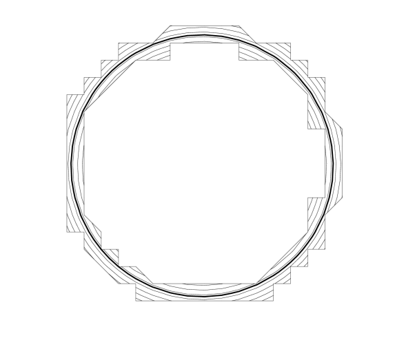
Figure 1: Isolines of the eigenfunction corresponding to the zero eigenvalue in the unstabilized method. Level set defining the circle drawn thicker.

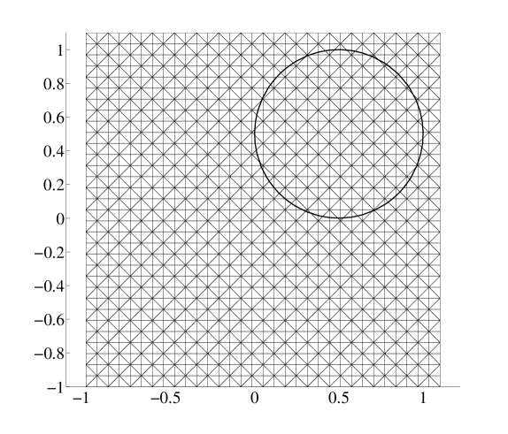
Figure 2: Level set isoline used to define the domain in a 2D mesh; initial position.

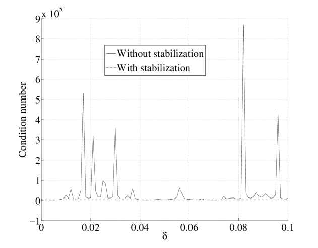
Figure 3: Condition numbers for the stabilized and unstabilized methods.

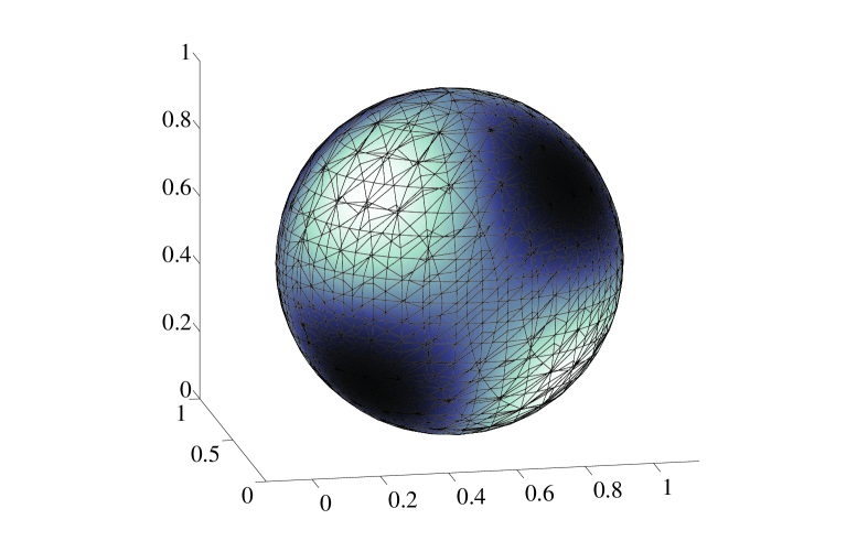
Figure 4: Discrete solution on a coarse mesh.

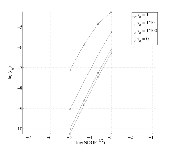
Figure 5: Convergence for different choices of $\tau_{0}$.

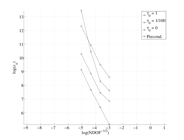
Figure 6: Condition numbers for different choices of $\tau_{0}$ and for preconditioning by diagonal scaling.

References

• [1] E. Burman and P. Hansbo. Fictitious domain finite element methods using cut elements: I. A stabilized Lagrange multiplier method. Comput. Methods Appl. Mech. Engrg., 199(41-44):2680–2686, 2010.
• [2] E. Burman and P. Hansbo. Fictitious domain finite element methods using cut elements: II. A stabilized Nitsche method. Appl. Numer. Math., 62(4):328–341, 2012.
• [3] K. Deckelnick, G. Dziuk, C. M. Elliott, and C.-J. Heine. An $h$-narrow band finite-element method for elliptic equations on implicit surfaces. IMA J. Numer. Anal., 30(2):351–376, 2010.
• [4] A. Demlow. Higher-order finite element methods and pointwise error estimates for elliptic problems on surfaces. SIAM J. Numer. Anal., 47(2):805–827, 2009.
• [5] A. Demlow and G. Dziuk. An adaptive finite element method for the Laplace-Beltrami operator on implicitly defined surfaces. SIAM J. Numer. Anal., 45(1):421–442, 2007.
• [6] G. Dziuk. Finite elements for the Beltrami operator on arbitrary surfaces. In Partial differential equations and calculus of variations, volume 1357 of Lecture Notes in Math., pages 142–155. Springer, Berlin, 1988.
• [7] G. Dziuk and C. M. Elliott. Eulerian finite element method for parabolic PDEs on implicit surfaces. Interfaces Free Bound., 10(1):119–138, 2008.
• [8] G. Dziuk and C. M. Elliott. Finite element methods for surface PDEs. Acta Numer., 22:289–396, 2013.
• [9] A. Ern and J.-L. Guermond. Evaluation of the condition number in linear systems arising in finite element approximations. ESAIM: Math. Model. Numer. Anal., 40(1):29–48, 2006.
• [10] D. Gilbarg and N. S. Trudinger. Elliptic partial differential equations of second order. Classics in Mathematics. Springer-Verlag, Berlin, 2001. Reprint of the 1998 edition.
• [11] A. Hansbo, P. Hansbo, and M. G. Larson. A finite element method on composite grids based on Nitsche’s method. ESAIM: Math. Model. Numer. Anal., 37(3):495–514, 2003.
• [12] P. Hansbo, M. G. Larson, and S. Zahedi. A cut finite element method for a stokes interface problem. Appl. Numer. Math., 85:90–114, 2014.
• [13] M. Lewicka and S. Müller. The uniform Korn-Poincaré inequality in thin domains. Ann. Inst. H. Poincaré Anal. Non Linéaire, 28(3):443–469, 2011.
• [14] A. Massing, M. G. Larson, A. Logg, and M. Rognes. A stabilized Nitsche fictitious domain method for the Stokes problem. J. Sci. Comput., 2014. DOI: 10.1007/s10915-014-9838-9.
• [15] M. A. Olshanskii and A. Reusken. A finite element method for surface PDEs: matrix properties. Numer. Math., 114(3):491–520, 2010.
• [16] M. A. Olshanskii, A. Reusken, and J. Grande. A finite element method for elliptic equations on surfaces. SIAM J. Numer. Anal., 47(5):3339–3358, 2009.
Refer to caption