Geometric Representation of Interacting Non-Relativistic Open Strings using Extended Objects

Abstract

Non-relativistic charged open strings coupled with Abelian gauge fields are quantized in a geometric representation that generalizes the Loop Representation. The model consists of open-strings interacting through a Kalb-Ramond field in four dimensions. The geometric representation proposed uses lines and surfaces that can be interpreted as an extension of the picture of Faraday’s lines of classical electromagnetism. This representation results to be consistent, provided the coupling constant (the “charge” of the string) is quantized. The Schrödinger equation in this representation is also presented.

I Introduction

In this paper we consider theories of non-relativistic strings interacting with an Abelian Kalb-Ramond field KR . The canonical quantization of the theory is made within the Dirac scheme for dealing with constrained theories, and a detailed discussion of issues as gauge invariance and the determination of the true degrees of freedom is presented. Then, we quantize the model in a representation that uses extended geometrical objets (paths and surfaces) that generalizes the usual Loop Representation ($LR$) GT . Special attention is devoted to the case of open strings, whose geometric representation requires the inclusion of open paths together with open surfaces in order to maintain gauge invariance, as we shall discuss. A ”surface representation” was considered years ago to study the free-field case Pio ; Pio2 , but it has to be adapted to include the particularities that the coupling with the string requires. This study can be seen as a generalization of the theory of charged non-relativistic point particles in electromagnetic interaction, quantized within the $LR$ , for which it was found that electric charge must be quantized in order to the $LR$ formulation be consistent Corichi1 ; Corichi2 ; E ; EP ; EA ; ED . As we shall see, both for the open and closed strings models coupled with the Kalb-Ramond field the “charge” of the string must be also quantized, if the geometric representation adapted to the model is going to be consistent. This result does not seem to be exclusive of the non-relativistic string case, but could be also reproduced for the relativistic one, since it is a consequence of the realization, in the ”surface representation”, of the ”generalized Gauss constraint”, which is the same in both the relativistic and non-relativistic cases.

In the next section we consider the model of a closed string in self-interaction by means of an Abelian Kalb-Ramond field KR ; EP ; EA ; ED ; the more interesting open string model is treated in an independent section. Final remarks and some discussions are made at the end of the paper.

II Non-relativistic self-interacting “charged” closed string: Surface representation.

Our discussion starts reviewing the case of a closed non-relativistic string in self-interaction EP ; ED , which is described by an action that generalizes the theory of the self-interacting point particle E

$$S=\frac{1}{12{g^{2}}}\int H^{\mu\nu\lambda}H_{\mu\nu\lambda}d^{4}x+\frac{\alpha}{2}\int dt\int d\sigma\left[(\dot{z}^{i})^{2}-(z^{\prime i})^{2})\right]+\frac{1}{2}\int d^{4}x\textit{J}^{\mu\nu}B_{\mu\nu},$$ (1)

where the Kalb-Ramond antisymmetric potential and field strength, $B_{\mu\nu}$ and $H_{\mu\nu\lambda}$, respectively, are related by $H_{\mu\nu\lambda}=3\partial_{[\mu}B_{\nu\lambda]}=\partial_{\mu}B_{\nu\lambda}+\partial_{\lambda}B_{\mu\nu}+\partial_{\nu}B_{\lambda\nu}$. The field $B_{\mu\nu}$ mediates the self-interaction of the closed string KR , so the Maxwell type term corresponds to its dynamical term. We have also a contribution corresponding to the free non-relativistic closed string, whose world sheet spatial coordinates $z^{i}(t,\sigma)$ are given in terms of the time $t$ and the parameter $\sigma$ along the string. The string tension $\alpha$ has units of $mass^{2}$ and $g$ is a parameter with units of $mass$. The string-field interaction term is given by means of the current

$$\textit{J}^{\mu\nu}(\vec{x},t) = \phi\int d\tau\int d\sigma\left[\dot{z}^{\mu}z^{\prime\nu}-\dot{z}^{\nu}z^{\prime\mu}\right]\delta^{(4)}(x-z)$$ (2)

$$\equiv \int d\sigma{\cal{J}}^{\mu\nu}(t,\sigma)\delta^{(3)}(\vec{x}-\vec{z}(t,\sigma)).$$

Here $\phi$ is a dimensionless coupling constant (analog to the charge in the case of particles), and we indicate with dots and primes partial derivation with respect to the parameters $\tau$ and $\sigma$, respectively. We take $\dot{z}^{0}=1$ and $z^{\prime 0}=0$. The interaction term can be written as

$$S_{int}=\frac{1}{2}\int dt\int d\sigma{\cal{J}}^{\mu\nu}(t,\sigma)B_{\mu\nu}(\vec{z}(t,\sigma)).$$ (3)

The action (1) is invariant under the gauge transformations $\delta B_{\mu\nu}=2\partial_{[\mu}\lambda_{\nu]}=\partial_{\mu}\lambda_{\nu}-\partial_{\nu}\lambda_{\mu}$, provided the string is closed.

We are interested in the Dirac quantization scheme of the theory. In this sense we observe that $B_{0i}$ is a non-dynamical variable, so we define the conjugate momenta associated to the fields, $B_{ij}$, and string variables, $z^{i}$, as

$$\Pi^{ij}=\frac{1}{2g^{2}}\left(\dot{B}_{ij}+\partial_{j}B_{0i}-\partial_{i}B_{0j}\right),\quad\quad P_{i}=\alpha\dot{z}^{i}+\phi B_{ij}z^{\prime j},$$ (4)

and obtain the Hamiltonian performing a Legendre transformation in the dynamical variables $B_{ij}$ and $z^{i}$,

$$H=\int d^{3}x\left[{g}^{2}\Pi^{ij}\Pi^{ij}+\frac{1}{12g^{2}}H_{ijk}H_{ijk}\right] + \int d\sigma\frac{\alpha}{2}\left[\frac{1}{\alpha^{2}}\left(P_{i}-\phi B_{ij}(z)z^{\prime j}\right)^{2}+(z^{\prime i})^{2}\right]+$$ (5)

$$+ \int d^{3}xB_{0i}\chi^{i},$$

where the role of $B_{0i}$ becomes clear as Lagrange multipliers enforcing the constraints

$$\chi^{i}(x)\equiv-\rho^{i}(x)-2\partial_{j}\Pi^{ji}(x))=0.$$ (6)

Here, $\rho^{i}(x)\equiv\phi\int d\sigma z^{\prime i}\delta^{(3)}(\vec{x}-\vec{z})$ ($=J^{0i}(x)$) is the “charge density” of the string. The preservation of the above constraints can be done using the canonical Poisson algebra of the fields involved. The non-vanishing Poisson brackets are given by

$$\left\{z^{i}(\sigma),P_{j}(\sigma^{\prime})\right\}=\delta^{i}_{j}\delta(\sigma-\sigma^{\prime}),$$ (7)

$$\left\{B_{ij}(\vec{x}),\Pi^{kl}(\vec{y})\right\}=\frac{1}{2}\left(\delta_{i}^{k}\delta_{j}^{l}-\delta_{i}^{l}\delta_{j}^{k}\right)\delta^{(3)}(\vec{x}-\vec{y}).$$ (8)

The preservation of the constraints does not produce new ones, and the $B_{0i}$ remain undetermined. This tells us that the constraints are first class (as can be directly verified by calculating their Poisson brackets) and generate time independent gauge transformations.

The basic observables, in the sense of Dirac, that can be constructed from the canonical variables, are the generalized electric and magnetic fields

$$\Pi^{ij} = \frac{1}{2g^{2}}H_{0ij}\equiv\frac{1}{2g^{2}}E^{ij},$$ (9)

B $$\equiv \frac{1}{3!}\epsilon^{ijk}H_{ijk},$$ (10)

the position $z^{i}(\sigma)$, and the covariant momentum of the string

$$P_{i}-\phi B_{ij}(z)z^{\prime j}.$$ (11)

All the physical observables of the theory are built in terms of these gauge invariant quantities, as can be verified. For instance, the Hamiltonian, given in equation (5), fulfils this requirement.

To quantize, we promote the canonical variables to operators that obey a conmutator algebra that results from the replacement $\{\quad,\quad\}\to-i[\quad,\quad]$, as usual. These operators have to be realized in a Hilbert space whose physical states $|\Psi\rangle_{Phys}$ are in the kernel of the constraint $\chi^{i}$

$$\chi^{i}|\Psi\rangle_{Phys}=0.$$ (12)

Now, in order to solve relation (12), a geometric representation adapted to the present model is introduced. This representation, based on extended objects, will be a “surface representation” related with the $LR$ formulated by Gambini and Trías GT , and with an early geometrical formulation of the pure Kalb-Ramond field based on closed surfaces Pio ; Pio2 . Consider the space of piecewise smooth oriented surfaces in $R^{3}$. A typical element of this space, let us say $\Sigma$, will be the union of several surfaces, with some of them being closed. In the space of smooth oriented surfaces $\Sigma$ we define equivalence classes of surfaces that share the same “form factor” $T^{ij}(x,\Sigma)=\int d\Sigma^{ij}_{y}\,\delta^{(3)}(\vec{x}-\vec{y})$, where $d\Sigma^{ij}_{y}=(\frac{\partial y^{i}}{\partial s}\frac{\partial y^{j}}{\partial r}-\frac{\partial y^{i}}{\partial r}\frac{\partial y^{j}}{\partial s})dsdr$ is the surface element and $s$, $r$ are the parametrization variables. All the features of the “open surfaces space”, are generalizations of aspects already present in the Abelian path space GT ; EP ; LO ; C ; EA ; ED .

Our Hilbert space is composed by functionals $\Psi(\Sigma)$ depending on equivalence classes $\Sigma$. We need to introduce the surface derivative $\delta_{ij}(x)$ defined by,

$$\Psi(\delta\Sigma\cdot\Sigma)-\Psi(\Sigma)=\sigma^{ij}\delta_{ij}(x)\Psi(\Sigma)$$ (13)

that measures the response of $\Psi(\Sigma)$ when an element of surface whose infinitesimal area $\sigma_{ij}=u^{i}v^{j}-v^{j}u^{i}$, generated by the infinitesimal vectors $\vec{u}$ and $\vec{v}$, is attached to $\Sigma$ at the point $x$ Pio ; Pio2 ; EP ; EA ; ED .

It can be seen that the fundamental commutator associated to relation (8) can be realized on surface-dependent functionals if one sets

$$\hat{\Pi}^{ij}(\vec{x})\longrightarrow\frac{1}{2}T^{ij}(\vec{x},\Sigma),$$ (14)

$$\hat{B}_{ij}(\vec{x})\longrightarrow 2i\delta_{ij}(\vec{x}),$$ (15)

since the surface-derivative of the form factor is given by

$$\delta_{ij}(\vec{x})T^{kl}(\vec{y},\Sigma)=\frac{1}{2}\left(\delta_{i}^{k}\delta_{j}^{l}-\delta_{i}^{l}\delta_{j}^{k}\right)\delta^{(3)}(\vec{x}-\vec{y}).$$ (16)

In this sense the states of the interacting theory can be taken as functionals $\Psi[\Sigma,z(\sigma)]$, where the field is represented by the surface $\Sigma$ and matter by means of the coordinates of the string world sheet. On the other hand, the operators associated to the string can be realized onto these functionals $\Psi[\Sigma,z(\sigma)]$ as follows

$$\hat{z}^{i}(\sigma)\longrightarrow z^{i}(\sigma),\quad\hat{P}^{i}(\sigma)\longrightarrow-i\frac{\delta}{\delta z^{i}(\sigma)}.$$ (17)

The operators of the theory are then realized in a representation that is the tensor product of the ”open-surface” representation, for the the field operators and a ”shape” representation for the string operators. Of all of these functionals we choose, as we stated, those that belong to the kernel of the generalized Gauss constraint (6), now written as

$$\left(-\rho^{i}(\vec{x})-2\partial_{j}\Pi^{ji}(\vec{x})\right)\Psi[\Sigma,z(\sigma)] \approx 0$$

$$\left(-\phi\int_{string}d\sigma z^{\prime i}\delta^{(3)}(\vec{x}-\vec{z})+\int_{\partial\Sigma}d\sigma z^{\prime i}\delta^{(3)}(\vec{x}-\vec{z})\right)\Psi[\Sigma,z(\sigma)] \approx 0.$$ (18)

In the last equation we have used that $\partial_{j}T^{ji}(\vec{x},\Sigma)=-T^{i}(\vec{x},\partial\Sigma)=-\int_{\partial\Sigma}dz^{i}\delta^{(3)}(\vec{x}-\vec{z})$, with $\partial\Sigma$ being the boundary of the surface.

If the oriented surface is such that its boundary coincides with the orientation of the string, the constraint reduces to $\left(\phi-1\right)\,\int_{string}d\sigma z^{\prime j}\delta^{(3)}(\vec{x}-\vec{z})=0$, and it is satisfied in general for $\phi=1$. We say in this case that the surface “emanates” or “starts” from the string, in analogy with the theory of self-interacting non-relativistic particles coupled through a Maxwell field E ; EA . It could happen instead, that the boundary of the surface and the string have opposite orientations; in that case the constraint would be satisfied if $\phi=-1$, and we say that the surface “enters” or “arrives” at the string position. There exist also the possibility that the surface could be composed by several layers ($n$ of them) that start (or end) at the string. Equation (II) becomes $\left(\phi-n\right)\,\int_{string}d\sigma z^{\prime j}\delta^{(3)}(\vec{x}-\vec{z})=0$, and in this case the coupling constant (“charge” of the string) must obey $\phi=n$ (the sign of $n$ depends on the fact that the surfaces may “emanate” from or “arrive” to the source). This is what we call a representation of “Faraday’s surfaces” for the string-Kalb-Ramond system, in analogy with the particle-Maxwell case. Finally, it should be remarked that when $\phi=n$, the surface may consist of the $n$ layers attached to the string, plus an arbitrary number of closed surfaces, since the latter do not contribute to the boundary of the surface that define the equivalence class $\Sigma$.

III Open strings: Surface$+$Path representation.

With this insight we move to the main subject of this paper, the model of open non-relativistic self-interacting strings. Our starting point will be the action,

$$\mathcal{S} = \int dt\int d\sigma\frac{\alpha}{2}[(\dot{z}^{i})^{2}-(z^{\prime i})^{2}]+$$ (19)

$$\qquad\qquad+\int d^{4}x\left(\frac{1}{12g^{2}}H^{\mu\nu\lambda}H_{\mu\nu\lambda}-\frac{m^{2}}{4}a^{\mu\nu}a_{\mu\nu}+\frac{1}{2}J^{\mu\nu}B_{\mu\nu}+J^{\mu}A_{\mu}\right),$$

where we have defined the $2$-form $a_{\mu\nu}=B_{\mu\nu}+F_{\mu\nu}$ with $F_{\mu\nu}=\partial_{\mu}A_{\nu}-\partial_{\nu}A_{\mu}$ as in the Stückelberg gauge invariant version of the Proca model E ; EA . The vector field $A_{\mu}$ has dimensions of $mass$, as in Maxwell theory, and mediates the interaction between the ends of the string. The Kalb-Ramond antisymmetric potential and field strength are related as before. The parameter $m$ is dimensionless.

The gauge field terms in (19) resemble the model for open strings proposed by Kalb and Ramond KR . The action is invariant under the simultaneous gauge transformations,

$$B_{\mu\nu}\;\longrightarrow\;B_{\mu\nu}+\partial_{\mu}\Lambda_{\nu}-\partial_{\nu}\Lambda_{\mu}\,,\qquad A_{\mu}\;\longrightarrow\;A_{\mu}-\Lambda_{\mu}+\partial_{\mu}\Lambda\,$$ (20)

only if the currents associated to the matter source (the body and the ending points of the string) satisfy the relation

$$\partial_{\mu}J^{\mu\nu}+J^{\nu}=0,$$ (21)

which emerges as a consequence of enforcing the equations of motion to be gauge invariant. There is still a residual gauge invariance in the gauge parameters ($\delta\Lambda_{\mu}=\partial_{\mu}\lambda$, $\delta\Lambda=\lambda$) that can be removed if we state that the gauge function $\Lambda_{\mu}$ is transverse (see the Appendix for further comments) .

The source condition (21) implies that the current associated to the endpoints is conserved ($\partial_{\nu}J^{\nu}=0$), even if the string-current $J^{\mu\nu}$ is not. This is a consequence of the form of the string interaction term, which has two types of currents associated to matter: one that is associated to the “body” and the other to the end points of the string. This fact permits the treatment of open-strings without losing gauge invariance. The source that couples with the Kalb-Ramond field is given by equation (2) as before, while the source that couples with the vector field is

$$\textit{J}^{\mu}(\vec{x},t) = e\int dz^{\mu}\delta^{(4)}(x-z){\mid}^{z_{f}}_{z_{i}},$$ (22)

$$\equiv \int d\sigma{\cal{J}}^{\mu}(t,\sigma)\delta^{(3)}(\vec{x}-\vec{z}(t,\sigma)),$$

where we defined ${\cal{J}}^{\mu}(t,\sigma)\equiv e\dot{z}^{\mu}(t,\sigma)(\delta(\sigma-\sigma_{f})-\delta(\sigma-\sigma_{i}))$ (with $\dot{z}^{0}=1$), and the subscripts $i$ and $f$ identify the initial and final points of the string. The vector source can be thought as two opposite charges attached to the ends of the open string. It can be checked that the sources satisfy the constraint (21), provided that $\phi=-e$. In the case of more than one open string the generalization is straightforward.

The equations of motion that arise from (19) are

$$\frac{1}{g^{2}}\partial_{\lambda}H^{\lambda\mu\nu}+m^{2}a^{\mu\nu}-J^{\mu\nu} = 0,$$ (23)

$$m^{2}\partial_{\lambda}a^{\lambda\mu}+J^{\mu} = 0,$$ (24)

$$\alpha(z^{\prime\prime i}-\ddot{z}^{i})+\frac{1}{2}H_{i\mu\nu}(z){\cal{J}}^{\mu\nu}(t,\sigma)+F_{i\mu}(z){\cal{J}}^{\mu}(t,\sigma) = 0$$ (25)

and they guarantee that (21) is satisfied, in order to be gauge invariant under (20). From (23) and (24) we obtain that the excitations are massive

$$(\Box+m^{2}g^{2})a^{\mu\nu}=g^{2}{\textit{J}}^{\mu\nu}-\frac{1}{m^{2}}(\partial^{\mu}\textit{J}^{\nu}-\partial^{\nu}\textit{J}^{\mu}).$$ (26)

The field $A_{\mu}$ can be eliminated in virtue of the gauge invariance, in this sense it is said that the Maxwell photon is “absorbed” to obtain a massive pseudovector KR .

Now, we implement with the Dirac quantization procedure. We take $A_{i}$, $B_{ij}$ and $z^{i}$ as dynamical variables and $\Pi^{i}$, $\Pi^{ij}$ and $P_{i}$ as their canonical conjugate momenta, respectively. After a Legendre transformation in the dynamical variables the Hamiltonian results to be

$$H = \int d^{3}x\left[g^{2}\Pi^{ij}\Pi^{ij}+\frac{1}{2m^{2}}\Pi^{i}\Pi^{i}+\frac{1}{12g^{2}}H_{ijk}H_{ijk}+\frac{m^{2}}{4}a_{ij}a_{ij}+A_{0}\Theta+B_{0i}\Theta^{i}\right]+$$ (27)

$$+\int d\sigma\frac{\alpha}{2}\left\{\frac{1}{\alpha^{2}}\left[P_{i}-\phi B_{ij}(z)z^{\prime j}-eA_{i}(z)\left(\delta(\sigma-\sigma_{f})-\delta(\sigma-\sigma_{i})\right)\right]^{2}+(z^{\prime i})^{2}\right\},$$

where, in analogy with the closed-string model, the fields variables $A_{0}$ and $B_{i0}$ appear in $H$ as Legendre multipliers enforcing the constraints

$$\Theta \equiv -\partial_{j}\Pi^{j}-J^{0}\approx 0,$$

$$\Theta^{i} \equiv -2\partial_{j}\Pi^{ji}-\Pi^{i}-J^{0i}\approx 0.$$ (28)

It can be seen that $\partial_{i}\Theta^{i}=\Theta$ when $\phi=-e$, hence, the constraints form a reducible set.

The usual Poisson algebra between the canonical conjugate variable is now defined. The non-vanishing brackets are

$$\{B_{ij}(\vec{x}),\Pi^{kl}(\vec{y})\} = \frac{1}{2}(\delta^{k}_{i}\delta^{l}_{j}-\delta^{l}_{i}\delta^{k}_{j})\delta^{(3)}(\vec{x}-\vec{y}),$$ (29)

$$\{A_{i}(\vec{x}),\Pi^{k}(\vec{y})\} = \delta^{k}_{i}\delta^{(3)}(\vec{x}-\vec{y}),$$ (30)

$$\{z^{i}(\sigma),P_{k}(\sigma^{\prime})\} = \delta^{i}_{k}\delta(\sigma-\sigma^{\prime}).$$ (31)

When the constraints are preserved no more constraints emerge and the Lagrange multipliers remain undetermined. So $\Theta$ and $\Theta^{i}$ turns out to be first class constraints that generates time independent gauge transformations on phase space. The generator of the infinitesimal gauge transformations is $G=\int d^{3}x(\Lambda\Theta+\Lambda_{i}\Theta^{i})$ and its effect on the dynamical fields is $\delta F=\{F,G\}$. The dynamical variables transform as follows

$$\delta A_{i}=\partial_{i}\Lambda-\Lambda_{i}\quad \quad\delta\Pi^{i}=0,$$ , (32)

$$\delta B_{ij}=\partial_{i}\Lambda_{j}-\partial_{j}\Lambda_{i}\quad \quad\delta\Pi^{ij}=0,$$ , (33)

$$\delta z^{i}=0\quad \quad\delta P_{i}=(\partial_{i}\Lambda_{k}(z)-\partial_{k}\Lambda_{i}(z)){\cal{J}}^{0k}+(\partial_{i}\Lambda(z)+\frac{\phi}{e}\Lambda_{i}(z)){\cal{J}}^{0},$$ , (34)

where it should be understood that $F(z)=\int d^{3}xF(x)\delta^{3}(\vec{x}-\vec{z})$. Using these transformations it can be seen that $H$ is gauge invariant as it is expected.

To count the number of degrees of freedom we note that we had initially $9$ dynamical fields ($A_{i}$, $B_{ij}$ and $z^{i}$) , subject to $3$ first class constraints ($\Theta$ and the transverse part of $\Theta_{i}$), or $4$ minus the reducibility condition, plus $3$ gauge conditions. This leave us with $2\times 9-2\times 3=12$ coordinates and conjugate momenta, corresponding to $6$ degrees of freedom, $3$ for the string coordinates ($z^{i}$) and $3$ for the massive pseudo vector field ($B_{ij}$). A further discussion of this subject and the gauge dependence of the model is presented in the Appendix at the end.

To quantize, as usual, the canonical variables are promoted to operators obeying the commutators that result from the replacement $\{\;,\;\}\;\longrightarrow\;-i[\;,\;]$. These operators have to be realized in a Hilbert space of physical states $|\Psi\rangle_{Phys}$, that obey the constraints (III) ($\Theta^{A}|\Psi\rangle_{Phys}=0$). The observables of the theory are constructed with gauge invariant objects.

At this point, we adapt a geometrical representation to the theory in terms of extended objects as it was done in the case of self interacting closed-strings. Now we take, besides the open surfaces associated to the Kalb-Ramond field, open paths $\gamma$ GT associated to the fields $A_{i}$, that mediate the interaction between the endpoints of the string. We prescribe,

$$\hat{B}_{ij}(\vec{x})\longrightarrow 2i\delta_{ij}(\vec{x}) \hat{\Pi}^{ij}(\vec{x})\longrightarrow\frac{1}{2}T^{ij}(\vec{x},\Sigma)$$ , (35)

$$\hat{A}_{i}(\vec{x})\longrightarrow i\delta_{i}(\vec{x}) \hat{\Pi}^{i}(\vec{x})\longrightarrow T^{i}(\vec{x},\gamma)$$ , (36)

where $T^{i}(\vec{x},\gamma)$ and and $T^{ij}(\vec{x},\Sigma)$ are the form factors that describes the open paths $\gamma$ and open surfaces $\Sigma$, respectively GT ; EP ; E . We can see, using $\partial_{j}T^{ji}(\vec{x},\Sigma)=-T^{i}(\vec{x},\partial\Sigma)$ and $\delta_{ij}(\vec{x})T^{lk}(\vec{y},\Sigma)=\frac{1}{2}(\delta^{l}_{i}\delta^{k}_{j}-\delta^{k}_{i}\delta^{l}_{j})\delta^{(3)}(\vec{x}-\vec{y})$, that the fundamental commutators associated to equations (29) and (30) can be realized when they act over functionals depending on both surfaces and paths. Also, the operators associated to the string can be realized in the same “shape” representation, as before. Henceforth, the states of the interacting theory can be taken as functionals $\Psi[\Sigma,\gamma,z(\sigma)]$ depending on geometric objects (open surfaces and paths) and the string coordinates $z^{i}(\sigma)$. Among these functionals, we must pick out those that belong to the kernel of the constraints (III), i.e., the physical space. In this representation they can be expressed as

$$\left(-\partial_{i}T^{i}(\vec{x},\gamma)-e\int d\sigma(\delta(\sigma-\sigma_{f})-\delta(\sigma-\sigma_{i}))\delta^{(3)}(\vec{x}-\vec{z})\right)\Psi[\Sigma,\gamma,z^{i}(\sigma)] \approx 0$$ (37)

$$\left(T^{i}(\vec{x},\partial\Sigma)-T^{i}(\vec{x},\gamma)+\phi\int_{\gamma_{s}}dz^{i}\delta^{(3)}(\vec{x}-\vec{z})\right)\Psi[\Sigma,\gamma,z^{i}(\sigma)] \approx 0,$$ (38)

with $\partial\Sigma$ being the boundary of $\Sigma$, and $\gamma_{s}$ is the path representing the string. The meaning of $\Sigma$ and $\gamma$ can be understood as follows. Given an open path $\gamma$ starting at $\vec{z}_{i}$ and ending at $\vec{z}_{f}$ it happens that $\partial_{i}T^{i}(\vec{x},\gamma)=-(\delta^{3}(\vec{x}-\vec{z}_{f})-\delta^{3}(\vec{x}-\vec{z}_{i}))$, so (37) is solved if $\gamma$ is attached to the endpoints of the string. If $e$ is positive the path should start at $\vec{z}_{i}$ and end at $\vec{z}_{f}$, which is consistent with the geometrical representation of non-relativistic particles in electromagnetic interaction EP , and the constraint gives $e=1$. In a more general sense $\gamma$ may consist of a bundle of open paths starting at $\vec{z}_{i}$ and ending at $\vec{z}_{f}$. In this case the charge has to be quantized and the number of paths depends on the value of $\mid e\mid$. It is clear that, since we are talking about equivalence classes of paths, the bundle of open paths could be accompanied by an additional number of loops that will not affect the interpretation. Looking at (38), we have that the relation $\partial_{i}\Theta^{i}=\Theta$ is satisfied, as we have seen, when $\phi=-e$ (or more generally when $\phi=q_{i}$ with $q_{i}$ the charge at the initial point of the string). On the other hand, and similarly to the closed-string case, we take $\Sigma$ as an open surface that has the string as part of his border, in such a way that if $\phi$ is positive the orientation of $\partial\Sigma$ and $\gamma_{s}$ coincide (when $\phi$ is negative their orientations are opposite). With this picture we see that, for $e$ positive, (38) is solved if $\partial\Sigma=\gamma+\overline{\gamma}_{s}$, where the overline on a path means the same path but with opposite orientation. We could have several open surfaces with the strings and the bundle of paths as their borders. The number of surfaces will depend on the absolute value of $e$ (or equivalently of $\phi$).

In a general situation we could have a group of open strings, enumerated with a subscript $a$ each of them, with quantized coupling constant $\phi_{a}$, in such a way that their endpoints can be thought as pairs of opposite charges. The “initial point” of each string has charge $q_{a}=\phi_{a}$. This guarantees that each source satisfies the constraint in order to preserve gauge invariance. The states of the theory correspond to functionals $\Psi[\Sigma,\gamma,z^{i}(\sigma)]$ that depends on open surfaces, open paths and the coordinates of the strings, where the open paths $\gamma$ are equivalence classes of a bundle of $\mid\phi_{a}\mid$ paths attached to the endpoints of the strings ending on the positive charge (outgoing from the negative charge). The open surface $\Sigma$ is a set of surfaces whose borders correspond to $\gamma$ and the strings. In figures 1 and 2 we show some examples of the surfaces $\Sigma$ and paths $\gamma$ that satisfy the gauge constraints. In figure 1 we show an example for 2 strings with one of them parametrized in such a way that the initial charge is positive. In figure 2 we present an example for 3 strings, one of them with charges $\pm 2e$ at its extremes. In the examples it is shown that the orientation of the surface $\Sigma$ coincides with the orientation of the parametrization of the string when the initial charge is positive and it is opposite when the initial charge is negative. This situation will be the same if we change the orientation of the parametrization. The other part of the border correspond to open paths that start on negative charges and end on positive charges in a number coincident with the multiplicity of charge $\pm e$. In 2 the string with charge $\pm 2e$ at its extremes (with $\phi=-2e$) belongs to part of the border of 2 open surfaces as it should. These cases are non unique, for example in the case of 2 strings there is another configuration with each string attached to part of the border of an open surface with the rest of the border corresponding to an open path connecting the extremes of the string. This configuration with 2 open surfaces is not topologically equivalent to the one presented in figure 1.

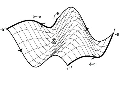
Figure 1: Surface-path representation example for 2 strings ($e>0$). The bold borders correspond to the strings.

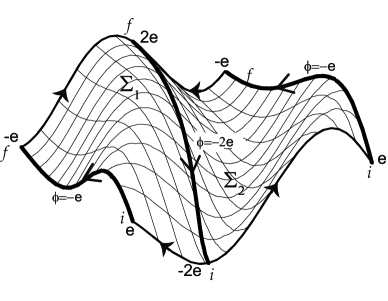
Figure 2: Surface-path representation for 3 strings ($e>0$). The bold borders correspond to the strings.

Finally we can write the Schrödinger equation in the path-surface representation. Taking into account $H$ in (27) acting on physical wave functionals, we write

$$-i\frac{\partial}{\partial t}\Psi[\Sigma,\gamma,z^{i}(\sigma)]=H\Psi[\Sigma,\gamma,z^{i}(\sigma)]$$

$$\qquad\qquad=\Bigg{\{}\int d^{3}x\left[\frac{1}{2g^{2}}\left((\frac{i}{3}\varepsilon^{ijk}\Delta_{ijk}(\vec{x}))^{2}+\frac{1}{2}E^{ij}E^{ij}\right)+\frac{1}{2m^{2}}T^{i}(\vec{x},\gamma)T^{i}(\vec{x},\gamma)+\right.$$

$$\qquad\qquad-\left.\left(\frac{m^{2}}{4}(2\delta_{ij}(\vec{x})+\Delta_{ij}(\vec{x}))(2\delta_{ij}(\vec{x})+\Delta_{ij}(\vec{x}))\right)\right]+$$

$$\qquad\qquad+\int d\sigma\frac{\alpha}{2}\left[\frac{1}{\alpha^{2}}\left(\frac{\delta}{\delta z^{i}(\sigma)}-2i\phi\delta_{ij}(\vec{z})z^{\prime i}(\sigma)-ie\delta_{i}(\vec{z})(\delta(\sigma-\sigma_{f})-\delta(\sigma-\sigma_{i}))\right)^{2}\right.$$

$$\qquad\qquad\qquad\qquad\qquad+(z^{\prime i}(\sigma))^{2}\Bigg{]}\Bigg{\}}\Psi[\Sigma,\gamma,z^{i}(\sigma)].$$ (39)

We see in (39) the free field contributions to the energy of the system, that appear as generalized Laplacians formed with surface and path derivatives, as well as quadratic terms containing form factors of paths and surfaces. The derivative terms come from the ”magnetic” operators B and $a_{ij}$

$$\textbf{B}\equiv\frac{1}{3!}\epsilon^{ijk}H_{ijk} \Rightarrow \textbf{B}=\frac{i}{3}\varepsilon^{ijk}\Delta_{ijk}(\vec{x}),$$ (40)

$$a_{ij} \Rightarrow i(2\delta_{ij}\left(\vec{x})+\Delta_{ij}(\vec{x})\right),$$ (41)

where we note the appearance of the closed surface derivative $\Delta_{ijk}(\vec{x})$ defined in Pio ; Pio2 and of a combined surface-loop derivative. This last combination takes into account that the open surface derivative alone is not gauge invariant, since paths are part of the boundary of surfaces, as discussed above. The “position” contributions come from $E^{ij}$ ($\rightarrow\frac{1}{2}T^{ij}(\vec{x},\Sigma)$) and $T^{i}(\vec{x},\gamma)$. Their should be regularized due to the appearance of Dirac delta functions products. The string contributions to the Hamiltonian comprise, besides terms corresponding to the kinetic and potential energy of the free string, the minimal coupling of the string variables with the Kalb-Ramond and vector fields. These appear as generalized Mandelstam derivatives, in the sense that as the functional $z^{i}(\sigma)$ derivative translates (infinitesimally) the string, the surface and path derivatives must also act in order to maintain the surface $\Sigma$ and its borders (paths and strings) joint together to preserve gauge invariance.

IV Discussion

We have studied a generalization of the $LR$ quantization of strings interacting by means of the Kalb-Ramond field. When the strings are closed, we saw that this representation is a “surface representation” that may be set up only if the coupling constant $\phi$ of the string (equivalent to the charge if we were dealing with point particles) is quantized, so it takes only integer values $n$. Hence, the theory is in a sense very similar to the Maxwell theory of interacting particles in the framework of the $LR$ E ; EP ; ED . There, the closed paths of the free Maxwell theory become open paths that start and end just where the charged particles are. In this sense, it is a “Faraday‘s lines representation”. It results then that both the electric flux carried by each Faraday‘s line and the electric charge are quantized in order to maintain gauge invariance. In the present study things are very similar. In both cases the appropriate Hilbert space is made of wave functionals whose arguments are geometric “Faraday‘s extended objects” (now surfaces) emanating from or ending at the strings (or particles) positions. The quantization of the “charge” of the particles or strings , i.e. the quantization of the coupling constant, is necessary to solve the first class Gauss constraint. In the case of $N$ strings, carrying different “charges” $\phi_{a}$, $a=1,..,N$, each string must be a source or sink of its own bundle of $n_{a}=\phi_{a}$ layers (these bundles may be accompanied by closed pieces of surfaces). This geometrical setting is possible if the couplings $\phi_{a}$ are quantized, since each individual sheet or layer carries a unit of Kalb-Ramond electric flux.

A step further, which is the main subject of this paper, is the case of the open string interaction. Now, in order to keep gauge invariance, we had to considerate separate couplings of gauge fields to the body and the endpoints of the strings. The corresponding geometric representation, in this case, yields the following picture. The states of the interacting theory of open strings can be taken as functionals $\Psi[\Sigma,\gamma,z(\sigma)]$ depending on surfaces and paths, and functions of the string variables $z(\sigma)$, that act as the source of the extended geometrical objects. The body of the string ”interacts” with a surface, that depending on the orientation of the string (i.e., the coupling constant $\phi$), “emanates” from or “arrives” to it. In turn, the endpoints of the string ”interact” via the open paths (just as in the case of electromagnetic interaction for particles) that complete the part of the border of the surface that is not “glued” to the strings. Again, as in the closed string interaction with the Kalb-Ramond field, the surface may consist of $n$ layers attached to the string (depending on the value of the coupling constant $\phi$), plus an arbitrary number of closed surfaces, since the latter do not contribute to the boundary of the surface. Each layer of open surface carries a unit of Kalb-Ramond flux emerging from or entering to a string, depending on the value of the string-charge $\phi$, and this is totally compatible with the number of open paths related to the endpoints of the string. This produces the quantization of the coupling constant of the strings. We have also presented the Schrödinger equation in the path-surface representation, analyzing the different terms that appear.

Following references EP ; LO ; ED ; Le ; W ; Wu ; In one could also consider the geometric representation of open strings interacting through topological terms, like a $BF$ term in $3+1$ dimensions. In these models the dependence of the wave-functionals on paths (or more generally, on the appropriate geometric objects that would enter in the representation) might be eliminated by means of an unitary transformation LO ; C ; Le . In that case one could obtain a quantum mechanics of particles, or particles and strings (depending on the model), subjected to long range interactions leading to anomalous statistics Wu ; In . This and other topics shall be the subject of future investigations.

V Appendix

In this Appendix we complete the discussion about gauge invariance of the open string model, and show how it can be expressed in a covariant way as it is expected from the original action (19).

After obtaining $H$ in (27) we saw that $A_{0}$ and $B_{0i}$ are lagrange multipliers associated with the first class constraints $\Theta$ and $\Theta^{i}$, and that the infinitesimal gauge transformations are generated by $G=\int d^{3}x(\Lambda\Theta+\Lambda_{i}\Theta^{i})$. The effect of gauge transformations on the dynamical fields was obtained in (32)-(34). The constraints are reducible ($\partial_{i}\Theta^{i}=\Theta$), so there is still a residual gauge invariance ($\delta\Lambda_{i}=\partial_{i}\lambda$, $\delta\Lambda=\lambda$) that manifests in $G$ itself. This residual invariance can be dealt with by asking $\Lambda_{i}$ to be transverse ($\partial^{i}\Lambda_{i}=0)$, and by absorbing the contribution due to the longitudinal part of $\Theta_{i}$ in in $\Lambda$. We can now proceed with the generator $\overline{G}=\int d^{3}x(\Lambda\Theta+{\Lambda^{T}}_{i}{\Theta^{T}}^{i})$, whose effect on the dynamical fields will be analogous to the former one, with ${\Lambda^{T}}_{i}$ instead of $\Lambda_{i}$ in (32)-(34). Hence we have two points of view about the issue of gauge invariance. In one of them we have a reducible set of constraints, with a residual gauge invariance. In the other one, we can deal with an irreducible set of constraints with no residual gauge invariance. The difference between both will appear, as we shall see, when we try to see how the multipliers change under gauge transformations.

In order to get a complete scheme of the gauge transformations we go to the extended action $S_{E}\sim\int dx(p\dot{q}-{\cal{H}})$ henneaux , consider the gauge transformation (32)-(34) with time dependent gauge parameters, and demand $S_{E}$ to be gauge invariant. Then, in the framework of the first point of view we get

$$\delta S_{E} = \int d^{4}x\left[\frac{d}{dt}\left(\Lambda(x)J^{0}(x)+\Lambda_{i}(x)J^{0i}(x)\right)\right.+$$ (42)

$$\qquad+\left.\left(\dot{\Lambda}-\delta A_{0}\right)\Theta+\left(\dot{\Lambda_{i}}-\delta B_{0i}\right)\Theta^{i}\right],$$

so the multipliers $A_{0}$ and $B_{0i}$ transform as $\delta A_{0}=\dot{\Lambda}$ and $\delta B_{0i}=\dot{\Lambda}_{i}$, provided that the gauge parameters satisfy

$$\int d^{3}x\left(\Lambda(x)J^{0}(x)+\Lambda_{i}(x)J^{0i}(x)\right){\mid}^{t_{f}}_{t_{i}}=0.$$ (43)

At this point the reducibility of the constraints plays now a role allowing an additional invariance on the multipliers: we can add to $B_{0i}$ the gradient of and scalar function ($\delta B_{0i}=-\partial_{i}\tilde{\Lambda}$) and simultaneously transform $A_{0}$ ($\delta A_{0}=-\tilde{\Lambda}$), leaving $S_{E}$ invariant. Taking all this into account we conclude that the action is invariant under the gauge transformations

$$\delta A_{\mu}=\partial_{\mu}\Lambda-\Lambda_{\mu}\qquad,\qquad\delta B_{\mu\nu}=\partial_{\mu}\Lambda_{\nu}-\partial_{\nu}\Lambda_{\mu},$$ (44)

where $\Lambda_{\mu}=(\tilde{\Lambda},\Lambda_{i})$.

Regarding the other point of view, we also go to the extended action with the modified gauge transformations (with $\Lambda_{i}$ replaced by $\Lambda^{T}_{i}$), which leads to

$$\delta S_{E} = \int d^{4}x\left[\frac{d}{dt}\left(\Lambda(x)J^{0}(x)+\Lambda^{T}_{i}(x)J^{0i}(x)\right)\right.+$$ (45)

$$\qquad+\left.\left(\dot{\Lambda}+\delta B^{L}-\delta A_{0}\right)\Theta+\left(\dot{\Lambda}^{T}_{i}-\delta B^{T}_{0i}\right){\Theta^{T}}^{i}\right],$$

where we have made the decomposition $\delta B_{0i}=\delta B^{T}_{0i}+\partial_{i}\delta B^{L}$. So we obtain the transformations $\delta A_{0}=\dot{\Lambda}-\delta B^{L}$ and $\delta B^{T}_{0i}=\dot{\Lambda}^{T}_{i}$. We note that a transverse vector $V^{T}_{\mu}$ ($\partial^{\mu}V^{T}_{\mu}=0$) can be written as $V^{T}_{\mu}=((-\Delta)V,V^{T}_{i}-\partial_{i}\dot{V})$ with $\partial^{i}V^{T}_{i}=0$. With this, the gauge transformations can be written as

$$\delta A_{0} = \partial_{0}\Lambda+\delta B^{L}=\partial_{0}(\Lambda-\dot{\overline{\Lambda}})+(\delta B^{L}+\ddot{\overline{\Lambda}}),$$

$$\delta B_{0i} = \partial_{0}\Lambda^{T}_{i}+\partial_{i}\delta B^{L}=\partial_{0}(\Lambda^{T}_{i}-\partial_{i}\dot{\overline{\Lambda}})+\partial_{i}(\delta B^{L}+\ddot{\overline{\Lambda}}),$$

$$\delta A_{i} = \partial_{i}\Lambda-\Lambda^{T}_{i}=\partial_{i}(\Lambda-\dot{\overline{\Lambda}})-(\Lambda^{T}_{i}-\partial_{i}\dot{\overline{\Lambda}}),$$

$$\delta B_{ij} = \partial_{i}\Lambda^{T}_{j}-\partial_{j}\Lambda^{T}_{i}=\partial_{i}(\Lambda^{T}_{j}-\partial_{j}\dot{\overline{\Lambda}})-\partial_{j}(\Lambda^{T}_{i}-\partial_{i}\dot{\overline{\Lambda}}),$$ (46)

where we have introduced $\overline{\Lambda}$ such that $\delta B^{L}=-\square\overline{\Lambda}$. In this sense the action is invariant under the gauge transformations

$$\delta A_{\mu}=\partial_{\mu}\lambda-\lambda^{T}_{\mu}\qquad,\qquad\delta B_{\mu\nu}=\partial_{\mu}\lambda^{T}_{\nu}-\partial_{\nu}\lambda^{T}_{\mu},$$ (47)

with $\lambda^{T}_{\mu}=((-\Delta)\overline{\Lambda},\Lambda^{T}_{i}-\partial_{i}\dot{\overline{\Lambda}})$. These parameters satisfy the condition

$$\int d^{3}x\left(\lambda(x)J^{0}(x)+\lambda^{T}_{i}(x)J^{0i}(x)\right){\mid}^{t_{f}}_{t_{i}}=0.$$ (48)

In the two point of views we can eliminate $A_{\mu}$ and the resulting action can be rewritten, using (21), in terms of only $a_{\mu\nu}$ as

$$\mathcal{S} = \int dt\int d\sigma\frac{\alpha}{2}[(\dot{z}^{i})^{2}-(z^{\prime i})^{2}]+$$ (49)

$$+\int d^{4}x\left(\frac{1}{12g^{2}}H^{\mu\nu\lambda}(a)H_{\mu\nu\lambda}(a)-\frac{m^{2}}{4}a^{\mu\nu}a_{\mu\nu}+\frac{1}{2}J^{\mu\nu}a_{\mu\nu}\right).$$

So we are left with an action in terms of $a_{\mu\nu}$ and the string coordinates $z^{i}$ with no further gauge invariance. The field $a_{\mu\nu}$ describes a massive excitation of mass $\mid gm\mid$.

Acknowledgements

This work was supported by Project $G-2001000712$ of FONACIT and Project PG 03-6039-2005 of CDCH-UCV.

References

- (1) M. Kalb and P. Ramond, “Classical Direct Interstring Action”, Phys. Rev. D 9,2273 (1974).
- (2) R. Gambini and A. Trias, “Second Quantization Of The Free Electromagnetic Field As Quantum Mechanics In The Loop Space”, Phys. Rev. D 22, 1380 (1980). “On The Geometrical OriginOf Gauge Theories”, Phys. Rev. D 23, 553 (1981). “Chiral Formulation Of Yang-Mills Equations: A Geometric Approach”, Phys. Rev. D 27, 2935 (1983). “Gauge Dynamics In The C Representation”, Nucl. Phys. B 278, 436 (1986). X. Fustero, R. Gambini and A. Trias, “Einstein’s Gravitation As A Gauge Theory Of The Lorentz Group”, Phys. Rev. D 31, 3144 (1985). C. di Bartolo, F. Nori, R. Gambini and A. Trias, “Loop Space Quantum Formulation Of Free Electromagnetism”, Lett. Nuovo Cim. 38, 497 (1983). R. Gaitan and L. Leal, “A geometric representation for the Abelian B-F term coupled to nontopological fields”, Int. J. Mod. Phys. A 11, 1413 (1996).
- (3) P.J. Arias, “Cuantización del Campo Antisimétrico de Calibre de Segundo Orden en el Espacio de Superficies”, Trabajo Especial de Grado, USB, 1985.
- (4) P. J. Arias, C. Di Bartolo, X. Fustero, R. Gambini and A. Trias, “Second quantization of the antisymmetric potential in the Abelian surfaces space”, Int. J. Mod. Phys. A 7, 737 (1992).
- (5) A. Corichi and K. V. Krasnov, “Loop quantization of Maxwell theory and electric charge quantization”, [arXiv:hep-th/9703177].
- (6) E. Fuenmayor, L. Leal and R. Revoredo, “Loop representation of charged particles interacting with Maxwell and Chern-Simons fields”, Phys. Rev. D 65, 065018 (2002).[arXiv:hep-th/0107013]
- (7) P. J. Arias, E. Fuenmayor and L. Leal, “Interacting particles and strings in path and surface representations”, Phys. Rev. D 69, 125010 (2004). [arXiv:hep-th/0402224]
- (8) E. Fuenmayor,“Charged particles and strings, interacting through Abelian Gauge fields in a Geometric Representation”, in spanish, Monography, 2003, UCV, Caracas, Venezuela.
- (9) E. Fuenmayor, “Study of Geometric Representations and Knot invariants in Topological Gauge theories coupled to matter”, In spanish, Doctoral Thesis, 2005, UCV,Caracas, Venezuela.
- (10) A. Corichi and K. V. Krasnov, “Ambiguities in loop quantization: Area vs. electric charge”, Mod. Phys. Lett. A 13, 1339 (1998).
- (11) L. Leal and O. Zapata, “Maxwell-Chern-Simons theory in a geometric representation,” Phys. Rev. D 63, 065010 (2001) [arXiv:hep-th/0008049].
- (12) J. Camacaro, R. Gaitan and L. Leal, “A geometric representation for the Proca model”, Mod. Phys. Lett. A 12 (1997) [arXiv:hep-th/9606121]; R. Gaitan and L. Leal, “A geometric representation for the Abelian B-F term coupled to nontopological fields”, Int. J. Mod. Phys. A 11, 1413 (1996).
- (13) J. M. Leinas and J. Myrrheim, “On the theory of identical particles”,II Nuovo Cimento, 37, 1 (1977)
- (14) F. Wilczek, “Magnetic flux, angular momentum and statistics”, Phys. Rev. Lett. 48, 1144 (1982); “Quantum mechanics of fractional spin particles”, Phys. Rev. Lett. 49, 957 (1982);Y. H. Chen, F. Wilczek, E. Witten and B. I. Halperin, “On anyon supeerconductivity”, Int. Jour. Mod. Phys. B3, 1001 (1989)
- (15) Y. S. Wu, “General thepry of quantum statistics in two-dimensions” Phys. Rev. Lett. 52, 2103 (1984); “Multiparcle quantum mechanics obeying fractional statistics”, Phys. Rev. Lett. 53, 111 (1984)
- (16) S. Rao, “An Anyon primer”. Lectures given at SERC school at Physyca Research Lab., Ahmedabad, Dec. 1991. [arXiv:hep-th/9209066].
- (17) M. Henneaux and C. Teitelboim, “Quantization of gauge systems”, Princeton University Press, New Jersey, 1992.