Precision calculation of the quartet-channel $p$–$d$ scattering length

Abstract

We present a fully perturbative calculation of the quartet-channel proton–deuteron scattering length up to next-to-next-to-leading order in pionless effective field theory. We use a framework that consistently extracts the Coulomb-modified effective range function for a screened Coulomb potential in momentum space and allows for a clear linear extrapolation back to the physical limit without screening. Our result of ${{}^{4}a}_{\text{$p$--$d$}}=(10.9\pm 0.4)~{}\mathrm{fm}$ agrees with older experimental determinations of this quantity but deviates from potential-model calculations and a more recent result from Black et al., which find larger values around $14~{}\mathrm{fm}$. As a possible resolution to this discrepancy, we discuss the scheme dependence of Coulomb subtractions in a three-body system.

I Introduction

The quartet-channel proton–deuteron scattering length ${{}^{4}a}_{\text{$p$--$d$}}$ is a fundamental observable in the nuclear three-body sector. The most recent determination of this quantity was carried out by Black et al. in Ref. Black:1999ab . Including a new measurement of the $p$–$d$ cross section performed at Triangle Universities Nuclear Laboratory (TUNL) for very low proton center-of-mass energies of only 163 and 211 $\mathrm{keV}$, they extracted a value of ${{}^{4}a}_{\text{$p$--$d$}}=(14.7\pm 2.3)~{}\mathrm{fm}$. While this falls in line with theoretical extractions of the quantity based on potential-model calculations Berthold:1986zz ; Chen:1991zza ; Kievsky:1997jd that find values for ${{}^{4}a}_{\text{$p$--$d$}}$ close to about $13.8~{}\mathrm{fm}$ (see Table 1 in Ref. Black:1999ab for details), it deviates quite significantly from older experimental determinations of ${{}^{4}a}_{\text{$p$--$d$}}$ that find values between $(11.11^{+0.25}_{-0.24})~{}\mathrm{fm}$ Huttel:1983ab and $(11.88^{+0.4}_{-0.1})~{}\mathrm{fm}$ Arvieux:1973ab (cf. Table 2 in Ref. Black:1999ab ). As a contribution to resolving this discrepancy, we present a new theoretical extraction of ${{}^{4}a}_{\text{$p$--$d$}}$ in pionless effective field theory, which only relies on two-body deuteron parameters as input. Our result obtained in a fully perturbative next-to-next-to-leading order calculation agrees quite well with the older experimental determinations. The key feature of our approach is a consistent numerical calculation of the Coulomb-modified effective range function that takes into account the screening of the Coulomb interaction by introducing a small photon mass in the momentum-space Skorniakov-Ter-Martirosian (STM) equation. As will be discussed below, we use a field-theoretical Coulomb subtraction scheme based on diagrammatic methods. We find a clearly linear (and weak) dependence of ${{}^{4}a}_{\text{$p$--$d$}}$ on the screening mass and can thus extrapolate back to the physical limit where the photon mass vanishes. The method described here can also be applied to other systems of charged particles. In particular, it should be interesting to use it together with the effective field theory for halo nuclei Bertulani:2002sz ; Bedaque:2003wa . When effective ranges are calculated as well, one can extract near-threshold bound-state properties such as asymptotic normalization constants from scattering parameters with relations as given, e.g., in Refs. Sparenberg:2009rv ; Koenig:2012bv . These constants can be used to determine the overall normalization of the S-factor for astrophysical nuclear reaction rates Gagliardi:1999aa .

II Pionless effective field theory

II.1 Overview

Effective field theories are a powerful theoretical tool that can be used to perform calculations of physical observables in terms of the relevant degrees of freedom. One such theory tailored specifically for few-nucleon systems at very low energies is the so called pionless effective field theory, which only includes short-range contact interactions between nucleons Kaplan:1998tg ; vanKolck:1998bw and is constructed to reproduce the effective range expansion Bethe:1949yr in the two-body system. As such, its expansion parameter $Q/\Lambda$, where $Q\sim\gamma_{d}\approx 45~{}\mathrm{MeV}$ is the typical momentum scale set by the deuteron binding momentum and $\Lambda=\mathcal{O}(m_{\pi})$ is the natural cutoff scale set by the left-out pion physics, can be directly related to the large $N$–$N$ scattering lengths and thus alternatively be written as $r_{0}/a$. A conservative estimate inserts for $r_{0}$ and $a$ the ${}^{3}S_{1}$ parameters $a\approx 5.42~{}\mathrm{fm}$ and $r_{0}\approx 1.75~{}\mathrm{fm}$ deSwart:1995ui , giving an EFT expansion parameter $\sim 1/3$. This means that at leading order (LO), next-to-leading order (NLO), and next-to-next-to-leading order (N²LO) one can expect results with about $30$, $10$, and $3$ percent accuracy, respectively.

In Refs. Bedaque:1997qi ; Bedaque:1998mb , the formalism has been extended to the spin-quartet $n$–$d$ system, whereas the inclusion of Coulomb effects was first done by Kong and Ravndal for the proton–proton channel Kong:1998sx ; Kong:1999sf and by Rupak and Kong Rupak:2001ci for the $p$–$d$ system. The ³He bound state was studied at leading order by Ando and Birse Ando:2010wq . In Ref. Konig:2011yq the present authors considered the ³He bound state as well as quartet- and doublet-channel $p$–$d$ scattering and in particular developed a numerical method to extract stable results at very low scattering energies. We build upon those results to extract ${{}^{4}a}_{\text{$p$--$d$}}$ as a threshold quantity.

The part of the pionless EFT Lagrangian that is relevant here can be written as

$$\!\!\mathcal{L}=N^{\dagger}\!\left(\mathrm{i}D_{0}+\frac{\boldsymbol{D}^{2}}{2M_{N}}\right)\!N-d^{i\dagger}\!\left[\sigma_{d}+\left(\mathrm{i}D_{0}+\frac{\boldsymbol{D}^{2}}{4M_{N}}\right)\right]\!d^{i}\\ +y_{d}\left[d^{i\dagger}\left(N^{T}P^{i}_{d}N\right)+\mathrm{h.c.}\right]+\mathcal{L}_{\mathrm{photon}}\,,$$ (1)

including a nucleon field $N$ (doublet in spin- and isospin space) and a single auxiliary dibaryon field $d^{i}$ corresponding to the deuteron with spin $1$ and isospin $0$. For the nucleon–deuteron quartet channel (total spin $\nicefrac{{3}}{{2}}$) this is all that enters up to N²LO in the $Q$ counting. In particular, it is not necessary to include an S–D-mixing term (generated by the spin-tensor operator in the nuclear force), which formally enters at N²LO but does not contribute to quartet-channel S-wave scattering at the zero-energy threshold.

To this order, the coupling to the electromagnetic field is determined by the covariant derivative $D_{\mu}=\partial_{\mu}+\mathrm{i}eA_{\mu}\hat{Q}$ with the charge operator $\hat{Q}$ and the photon field $A_{\mu}$, along with the kinetic term for the photons included in $\mathcal{L}_{\mathrm{photon}}$. For our nonrelativistic low-energy calculation it suffices to only keep the contribution of so-called Coulomb photons, corresponding to a static potential between charged particles. For convenience, this can be split up into a Coulomb-photon propagator $\mathrm{i}/(\mathbf{p}^{2}+\lambda^{2})$ and factors $(\pm\mathrm{i}e\,\hat{Q})$ for the vertices. More details on the formalism can be found in previous publications on the subject (see e.g.. Ref. Konig:2011yq ).

II.2 Full deuteron propagator

The bare deuteron propagator $\mathrm{i}/\sigma_{d}$ has to be dressed by nucleon bubbles to all orders in order to get the full leading-order expression Kaplan:1998tg ; vanKolck:1998bw . For convenience, one can also resum contributions from the kinetic term in Eq. (1). As is standard practice in the field, the result $\mathrm{i}\Delta_{d}(p_{0},\mathbf{p})$ is renormalized in the power divergence subtraction scheme Kaplan:1998tg by requiring the theory to reproduce the $n$–$p$ effective range expansion around the deuteron pole,

$${-y_{d}^{2}}\Delta_{d}\!\left(p_{0}=\frac{k^{2}}{2M_{N}},\mathbf{p}=0\right)=\frac{4\pi}{M_{N}}\frac{\mathrm{i}}{k\cot\delta_{d,t}-\mathrm{i}k}$$ (2)

with $k\cot\delta_{d}=-\gamma_{d}+\frac{\rho_{d}}{2}(k^{2}+\gamma_{d}^{2})+\,\cdots$, where we use $\gamma_{d}=\sqrt{M_{N}E_{d}}=45.7022(1)~{}\mathrm{MeV}$ vanderLeun:1982aa and $\rho_{d}=1.765(4)~{}\mathrm{fm}$ deSwart:1995ui . The sensitivity of our results to variations of $\gamma_{d}$ and $\rho_{d}$ within their errors is negligible. Note that the resummation of effective-range contributions in $\mathrm{i}\Delta_{d}(p_{0},\mathbf{p})$ has been introduced for convenience only and includes a subset of higher-order (N³LO etc.) terms Bedaque:2002yg . We furthermore define the deuteron wavefunction renormalization $Z_{0}$ as the residue of $\Delta_{d}$ at the bound-state pole, i.e., $Z_{0}=\gamma_{d}\rho_{d}/(1-\gamma_{d}\rho_{d})=\gamma_{d}\rho_{d}+(\gamma_{d}\rho_{d})^{2}+\cdots$.

Here, we carry out a strictly perturbative calculation that only includes terms up to a given order in the final result. This is desirable because it avoids the potentially problematic resummation of higher-order terms and thus allows for a complete control of theoretical corrections and a clean check of the expected convergence pattern. Adopting the approach introduced in Ref. Vanasse:2013sda for the $n$–$d$ system, we define $D_{d}(E;q)\equiv(-\mathrm{i})\cdot\Delta_{d}\left(E-q^{2}/(2M_{N}),q\right)$ and expand this as

$$D_{d}(E;q)=D_{d}^{(0)}(E;q)+D_{d}^{(1)}(E;q)+D_{d}^{(2)}(E;q)+\cdots=-\frac{4\pi}{M_{N}y_{d}^{2}}\frac{1}{-\gamma_{d}+\sqrt{3q^{2}/4-M_{N}E-\mathrm{i}\varepsilon}}\\ \times\left[1+\frac{\rho_{d}}{2}\frac{\left(3q^{2}/4-M_{N}E-\gamma_{d}^{2}\right)}{-\gamma_{d}+\sqrt{3q^{2}/4-M_{N}E-\mathrm{i}\varepsilon}}+\left(\frac{\rho_{d}}{2}\frac{\left(3q^{2}/4-M_{N}E-\gamma_{d}^{2}\right)}{-\gamma_{d}+\sqrt{3q^{2}/4-M_{N}E-\mathrm{i}\varepsilon}}\right)^{\!2}+\cdots\right]\,.$$ (3)

Here and in the following, the superscript in parentheses indicates the order (in $\rho_{d}$) of the individual parts.

II.3 Coulomb diagrams

From the strong sector of pionless EFT, we only have the simple one-nucleon-exchange interaction represented by the kernel

$$K_{\mathrm{s}}(E;k,p)\equiv\frac{1}{kp}\;Q_{0}\!\left(\frac{k^{2}+p^{2}-M_{N}E-\mathrm{i}\varepsilon}{kp}\right)\,,$$ (4)

where from S-wave projection one has the Legendre function of the second kind

$$Q_{0}(a)=\frac{1}{2}\int_{-1}^{1}\frac{\mathrm{d}x}{x+a}=\frac{1}{2}\ln\left(\frac{a+1}{a-1}\right)\,.$$ (5)

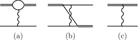
Figure 1: Leading $\mathcal{O}(\alpha)$ diagrams involving Coulomb photons.

As done in previous calculations Rupak:2001ci ; Konig:2011yq , we regulate the singularity of the Coulomb potential at zero momentum transfer by introducing a small photon mass $\lambda$. With the numerical technique described in Ref. Konig:2011yq , this regularization approach is well under control and it is possible to extrapolate results back to the physical limit $\lambda\to 0$. In Fig. 1 we show the relevant diagrams involving Coulomb photons. Of these, the “bubble diagram” in Fig. 1(a) is the most important one because it is both of leading order in the $Q/\Lambda$ counting and enhanced at low energies by the Coulomb pole. The corresponding interaction kernel $K_{\text{bub}}(E;k,p)$ is given by

$$K_{\text{bub}}(E;k,p)=-\alpha M_{N}\times\frac{1}{2}\int_{-1}^{1}\mathrm{d}\cos\theta\,\frac{\arctan\!\left(\frac{2\mathbf{p}^{2}-\mathbf{k}^{2}-\mathbf{k}\cdot\mathbf{p}}{\sqrt{3\mathbf{k}^{2}-4M_{N}E-\mathrm{i}\varepsilon}\sqrt{(\mathbf{k}-\mathbf{p})^{2}}}\right)+\arctan\!\left(\frac{2\mathbf{k}^{2}-\mathbf{p}^{2}-\mathbf{k}\cdot\mathbf{p}}{\sqrt{3\mathbf{p}^{2}-4M_{N}E-\mathrm{i}\varepsilon}\sqrt{(\mathbf{k}-\mathbf{p})^{2}}}\right)}{\left((\mathbf{k}-\mathbf{p})^{2}+\lambda^{2}\right)\sqrt{(\mathbf{k}-\mathbf{p})^{2}}}\,,$$ (6)

where $\theta$ is the angle between the momentum vectors $\mathbf{k}$ and $\mathbf{p}$. A detailed derivation of this expression can be found in Refs. Konig:2011yq ; Koenig:2013 ; Konig:2014ufa ; for an expression with the angular integration carried out explicitly, see Ref. Vanasse:2014kxa . In contrast to earlier work Rupak:2001ci ; Konig:2011yq , we do not approximate the bubble loop integral as a constant in this calculation but keep the full dynamical expression. The diagram shown in Fig. 1(c) also features the Coulomb pole, but since it is only generated by the deuteron kinetic term in the Lagrangian (1), it is formally an effective-range correction:

$$K_{\rho_{d}}(E;k,p)=-\alpha M_{N}\times\frac{\rho_{d}}{2kp}\;Q_{0}\!\left(-\frac{k^{2}+p^{2}+\lambda^{2}}{2kp}\right)\,.$$ (7)

Finally, we have the “box diagram” shown in Fig. 1(b), giving rise to the additional interaction kernel Hoferichter-BoxDiag:2010

$$K_{\text{box}}(E;k,p)=-\alpha M_{N}\\ \times\frac{1}{2}\int_{-1}^{1}\mathrm{d}\!\cos\theta\,\Bigg{\{}\frac{\arctan\!\Big{(}\frac{2\mathbf{p}^{2}-\mathbf{k}^{2}-\mathbf{k}\cdot\mathbf{p}}{\sqrt{3\mathbf{k}^{2}-4M_{N}E-\mathrm{i}\varepsilon}\sqrt{(\mathbf{k}-\mathbf{p})^{2}}}\Big{)}+\arctan\!\Big{(}\frac{2\mathbf{k}^{2}-\mathbf{p}^{2}-\mathbf{k}\cdot\mathbf{p}}{\sqrt{3\mathbf{p}^{2}-4M_{N}E-\mathrm{i}\varepsilon}\sqrt{(\mathbf{k}-\mathbf{p})^{2}}}\Big{)}}{(\mathbf{k}^{2}+\mathbf{p}^{2}+\mathbf{k}\cdot\mathbf{p}-M_{N}E-\mathrm{i}\varepsilon)\sqrt{(\mathbf{k}-\mathbf{p})^{2}}}\\ -\frac{\lambda}{(\mathbf{k}^{2}+\mathbf{p}^{2}+\mathbf{k}\cdot\mathbf{p}-M_{N}E-\mathrm{i}\varepsilon)^{2}}\Bigg{\}}+\mathcal{O}(\lambda^{2})\,,$$ (8)

as discussed in Refs. Koenig:2013 ; Konig:2014ufa ; Vanasse:2014kxa . According to the original counting of Rupak and Kong, this diagram formally scales like an NLO-correction. Refs. Koenig:2013 ; Konig:2014ufa suggest an alternative scheme that includes all $\mathcal{O}(\alpha)$ Coulomb diagrams at leading order, except for $K_{\rho_{d}}$ because it is proportional to the effective range. We will present here results for both schemes (and show that they agree within the EFT uncertainty).

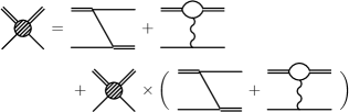
Figure 2: Integral equation for the full (i.e. strong + Coulomb) scattering quartet-channel amplitude $\mathcal{T}_{\mathrm{full}}$.

The STM equation for the system including both the one-nucleon-exchange and the Coulomb bubble diagram, shown diagrammatically in Fig. 2, can now be written as

$$\mathcal{T}_{\mathrm{full}}(E;k,p)=-M_{N}y_{d}^{2}\left[K_{s}(E;k,p)-\tfrac{1}{2}K_{\text{bub}}(E;k,p)\right]\\ +\frac{M_{N}y_{d}^{2}}{2\pi^{2}}\int_{0}^{\Lambda}\mathrm{d}q\,q^{2}\,\mathcal{T}_{\mathrm{full}}(E;k,q)\\ \times D_{d}(E;q)\left[K_{s}(E;q,p)-\tfrac{1}{2}K_{\text{bub}}(E;q,p)\right]\,.$$ (9)

In writing this, we have introduced an explicit momentum cutoff $\Lambda$. In the following, we will use an abbreviated notation where the arguments of the functions are suppressed:

$$\mathcal{T}_{\mathrm{full}}=-M_{N}y_{d}^{2}\left(K_{s}-\tfrac{1}{2}K_{\text{bub}}\right)\\ +\mathcal{T}_{\mathrm{full}}\otimes\left[M_{N}y_{d}^{2}\,D_{d}\left(K_{s}-\tfrac{1}{2}K_{\text{bub}}\right)\right]\,,$$ (10)

with $A\otimes B\equiv\frac{1}{2\pi^{2}}\int_{0}^{\Lambda}\mathrm{d}q\,q^{2}\,A(\ldots,q)B(q,\ldots)$. In the alternative scheme mentioned above, $K_{\text{box}}$ has to be added to the kernels in Eqs. (9), (10). Either way, for pure Coulomb scattering one simply has

$$\mathcal{T}_{\mathrm{c}}=\tfrac{1}{2}{M_{N}y_{d}^{2}}\,K_{\text{bub}}-\mathcal{T}_{\mathrm{c}}\otimes\left[\tfrac{1}{2}{M_{N}y_{d}^{2}}\,D_{d}K_{\text{bub}}\right]\,.$$ (11)

We note that due to the photon coupling to the two-nucleon bubble, both $\mathcal{T}_{\mathrm{c}}$ and the Coulomb-phase shift $\delta_{\mathrm{c}}$ extracted from $\mathcal{T}_{\mathrm{c}}$ include short-range three-body Coulomb contributions. Below, we will come back to a fully perturbative expansion of the form $\mathcal{T}(E;k,p)=\mathcal{T}^{(0)}(E;k,p)+\mathcal{T}^{(1)}(E;k,p)+\cdots$ for the amplitudes, and to the perturbative inclusion of the kernel function $K_{\rho_{d}}$.

III The Coulomb-modified scattering length

First, we introduce the quartet-channel $p$–$d$ scattering length, which is defined by the Coulomb-modified effective range expansion Bethe:1949yr (for a more detailed discussion, see Ref. Koenig:2012bv and further references therein), which we write here in the form

$$C_{\eta}^{2}\,k\cot\delta_{\mathrm{diff}}(k)+\gamma_{\text{$p$--$d$}}\,h(\eta)=-\frac{1}{a^{C}}+\frac{r^{C}}{2}k^{2}+\cdots\,,$$ (12)

where $\delta_{\mathrm{diff}}(k)=\delta_{\mathrm{full}}(k)-\delta_{\mathrm{c}}(k)$ is the Coulomb-subtracted phase shift, and $h(\eta)$ with $\eta=\gamma_{\text{$p$--$d$}}/(2k)$ and $\gamma_{\text{$p$--$d$}}=4\alpha M_{N}/3$ is a nonanalytic function of the momentum that we will discuss further below (it vanishes as $k\to 0$ and is thus not important to extract the scattering length in that limit). In Eq. (12), the “Gamow factor” $C_{\eta}^{2}=2\pi\eta/[\exp(2\pi\eta)-1]$ vanishes rapidly as $k\to 0$, while at the same time $k\cot\delta_{\mathrm{diff}}(k)$ has a pole in that limit. This means that a finite well-defined value for the scattering length relies on a rather delicate cancellation. In our numerical calculation with a finite photon mass $\lambda$ it is thus important to consistently extract a screened expression $C_{\eta,\lambda}^{2}$ and use this in Eq. (12). It can be shown Koenig:2013 that the answer to this problem is

$$C_{\eta,\lambda}^{2}=\left|1+\frac{2M_{N}}{3\pi^{2}}\int_{0}^{\Lambda}\frac{\mathrm{d}p\,p^{2}}{p^{2}-k^{2}-\mathrm{i}\varepsilon}Z_{0}\mathcal{T}_{\mathrm{c}}(E;p,k)\right|^{2}\,,$$ (13)

where $\mathcal{T}_{\mathrm{c}}(E;p,k)$ is the numerical solution of the STM equation with the screened Coulomb interaction, which is also used to calculate the pure Coulomb phase shift $\delta_{\mathrm{c}}(k)$. A detailed derivation of Eq. (13) can be found in Ref. Koenig:2013 . Here, we note that it is based on the modified effective range expansion derived in Ref. vanHaeringen:1982ab . For the generic case where the interaction is given by the sum of a long-range potential $V_{L}$ and a short-range interaction $V_{S}$, the effective-range function (K-matrix) can be written as

$$|\mathcal{F}_{\ell}(k)|^{-2}k^{2\ell+1}\left(\cot\delta_{\ell}^{M}(k)-\mathrm{i}\right)+M_{\ell}(k)\,,$$ (14)

where $\delta_{\ell}^{M}(k)$ is the subtracted phase shift for angular momentum $\ell$. $\mathcal{F}_{\ell}(k)$ is the Jost function associated with the long-range potential. For the unscreened Coulomb potential, one simply recovers $|\mathcal{F}_{0}(k)|^{-2}=C_{\eta}^{2}$. More generally, $|\mathcal{F}_{0}(k)|^{-2}$ is given by the two-particle scattering wavefunction at zero separation (see e.g. Ref. Newton:1982 ). Relating this then to the half off-shell T-matrix gives our Eq. (13). Finally, from the results derived by Kong and Ravndal for the proton–proton system Kong:1999sf , we know that for the unscreened Coulomb potential the function $h(\eta)=\mathrm{Re}\,\psi(\mathrm{i}\eta)-\ln|\eta|$ can be obtained from a momentum-space integral,

$$h(\eta)=\mathrm{Re}\,H(\eta)\\ =\mathrm{Re}\left\{-\frac{2\pi}{\alpha\mu}\int\!\!\frac{\mathrm{d}^{3}q}{(2\pi)^{3}}\frac{C_{\eta}^{2}(q)}{q^{2}}\frac{k^{2}}{k^{2}-q^{2}+\mathrm{i}\varepsilon}\right\}$$ (15)

for $\eta=\eta(k)$, and where $\mu$ is reduced mass $\mu$ (in Ref. Kong:1999sf , $\mu=M_{N}/2$). Generalizing this result, we set (with a principal-value integration)

$$h_{\lambda}(\eta)=\frac{k^{2}}{\alpha\mu}\frac{1}{\pi}\,\mathrm{P}\!\int_{0}^{\Lambda}\!\mathrm{d}q\,\frac{C_{\eta,\lambda}^{2}(q)}{(q+k)(q-k)}\ \ \text{,}\ \ \mu=2M_{N}/3$$ (16)

to take into account the remaining screening corrections. Note that although we have written $h_{\lambda}(\eta)$, the dependence is really on $k$ directly. The $C_{\eta,\lambda}^{2}(q)$ under the integral is calculated from Eq. (13) for each $q$. A key feature of this approach, which we believe is crucial for a consistent and stable extraction of observables, is that we are calculating the proper modified effective range function for the case where the screened Coulomb interaction is defined by the diagrams shown in Figs. 1(a) and (c). We thus expect the scaling with $\lambda$ to be well under control. Altogether, we get for the extraction of the quartet-channel $p$–$d$ scattering length ${{}^{4}a}_{\text{$p$--$d$}}$

$$C_{\eta,\lambda}^{2}\,k\cot\delta_{\mathrm{diff}}(k)+\gamma_{\text{$p$--$d$}}\,h_{\lambda}(\eta)=-\frac{1}{{{}^{4}a}_{\text{$p$--$d$}}}+\mathcal{O}(k^{2})\,.$$ (17)

Note that the $\gamma_{\text{$p$--$d$}}$ here cancels against the $\alpha\mu$ in Eq. (16), so that this scale eventually does not enter directly and we could in fact just define the correction term as a whole. Our convention here has been chosen to exhibit the connection to the modified effective range expansion for the unscreened Coulomb potential.

IV Fully perturbative calculation

As mentioned above, calculations beyond leading order can be performed in a numerically simple way by using deuteron propagators with (partially) resummed effective-range corrections. This was done in Ref. Konig:2011yq and other earlier works cited above. The arbitrary inclusion of higher-order contributions, however, can spoil the EFT convergence pattern and leads to uncertainties that are difficult to control. We thus carry out here a strictly perturbative calculation that only includes terms up to a given order in the final result. For the three-boson system such a calculation up to N²LO was presented by Ji and Phillips Ji:2012nj . Ref. Vanasse:2013sda introduced a new approach to carry out this calculation more efficiently by avoiding the need to determine the full off-shell scattering amplitude and applied this to the neutron–deuteron system in pionless EFT. Here, we apply that formalism to the proton–deuteron system. To this end, we separately expand the kernel of the STM equation in the effective range as $K(E;k,p)=K^{(0)}(E;k,p)+K^{(1)}(E;k,p)+\cdots$ with

$$K^{(0)} =-\frac{M_{N}y_{d}}{2}\left(2K_{\mathrm{s}}-K_{\text{bub}}\right)\,,$$ (18a)

$$K^{(1)} =-\frac{M_{N}y_{d}}{2}\left(K_{\rho_{d}}+K_{\text{box}}\right)\,,$$ (18b)

and $K^{(2)}=0$ since there is no new $\mathcal{O}(\rho_{d}^{2})$ kernel contribution. The alternative scheme mentioned below Eq. (7) includes $K_{\text{box}}$ in $K^{(0)}$. We then find the following set of equations for the contributions up to N²LO:

$$\mathcal{T}_{\mathrm{full}}^{(0)} =K^{(0)}+\mathcal{T}_{\mathrm{full}}^{(0)}\otimes D_{d}^{(0)}\,K^{(0)}$$ (19a)

$$\mathcal{T}_{\mathrm{full}}^{(1)} =K^{(1)}+\mathcal{T}_{\mathrm{full}}^{(0)}\otimes\left[D_{d}^{(0)}\,K^{(1)}+D_{d}^{(1)}\,K^{(0)}\right]$$ (19b)

$$\hskip 13.30003pt+\mathcal{T}_{\mathrm{full}}^{(1)}\otimes D_{d}^{(0)}\,K^{(0)}\,,$$

$$\mathcal{T}_{\mathrm{full}}^{(2)} =\mathcal{T}_{\mathrm{full}}^{(0)}\otimes\left[D_{d}^{(1)}\,K^{(1)}+D_{d}^{(2)}\,K^{(0)}\right]+\mathcal{T}_{\mathrm{full}}^{(1)}$$ (19c)

$$\hskip 13.30003pt\otimes\left[D_{d}^{(0)}\,K^{(1)}+D_{d}^{(1)}\,K^{(0)}\right]+\mathcal{T}_{\mathrm{full}}^{(2)}\otimes D_{d}^{(0)}\,K^{(0)}\,.$$

As in Ref. Vanasse:2013sda , this procedure calculates higher-order corrections by re-shuffling terms to the inhomogeneous parts of the integral equations. In our generalization to treat the case of charged particles, corrections arise not only from the expansion of the propagators, but also from additional interaction kernels at higher orders. Expressions analogous to those in Eqs. (19) are obtained for the perturbative parts of $\mathcal{T}_{\mathrm{c}}$ by simply dropping $K_{\mathrm{s}}$ and $K_{\text{box}}$. Combining this with the perturbative expansion of the deuteron wavefunction renormalization Griesshammer:2004pe , $Z_{0}=Z_{0}^{(0)}+Z_{0}^{(1)}+\cdots$, one obtains the physical T-matrices as $Z_{0}^{(0)}\mathcal{T}^{(0)}$, $Z_{0}^{(0)}\mathcal{T}^{(1)}+Z_{0}^{(1)}\mathcal{T}^{(0)}$ etc., and finally the perturbative expansion of $k\cot\delta_{\mathrm{diff}}(k)$ as

$$\left[k\cot\delta_{\mathrm{diff}}\right]^{(0)} =\frac{2\pi}{\mu}\frac{\mathrm{e}^{2\mathrm{i}\delta_{\mathrm{c}}^{(0)}}}{T_{\mathrm{diff}}^{(0)}}+\mathrm{i}k\,,$$ (20a)

$$\left[k\cot\delta_{\mathrm{diff}}\right]^{(1)} =\frac{2\pi}{\mu}\mathrm{e}^{2\mathrm{i}\delta_{\mathrm{c}}^{(0)}}\times\left[\frac{2\mathrm{i}\delta_{\mathrm{c}}^{(1)}}{T_{\mathrm{diff}}^{(0)}}-\frac{T_{\mathrm{diff}}^{(1)}}{(T_{\mathrm{diff}}^{(0)})^{2}}\right]\,,$$ (20b)

$$\left[k\cot\delta_{\mathrm{diff}}\right]^{(2)} =-\frac{2\pi}{\mu}\mathrm{e}^{2\mathrm{i}\delta_{\mathrm{c}}^{(0)}}\times\Bigg{[}\frac{2(\delta_{\mathrm{c}}^{(1)})^{2}-2\mathrm{i}\delta_{\mathrm{c}}^{(2)}}{T_{\mathrm{diff}}^{(0)}}$$ (20c)

$$\hskip 40.00006pt+\frac{2\mathrm{i}\delta_{\mathrm{c}}^{(1)}T_{\mathrm{diff}}^{(1)}+T_{\mathrm{diff}}^{(2)}}{(T_{\mathrm{diff}}^{(0)})^{2}}-\frac{(T_{\mathrm{diff}}^{(1)})^{2}}{(T_{\mathrm{diff}}^{(0)})^{3}}\Bigg{]}\,,$$

where $T_{\mathrm{diff}}=T_{\mathrm{full}}-T_{\mathrm{c}}$, $\mu=2M_{N}/3$, and analogous expressions for the phase shift $\delta_{\mathrm{c}}^{(n)}(k)$ that can be found, for example, in Ref. Vanasse:2013sda . For the application of Eq. (17) this still has to be combined with an analogous expansion of $C_{\eta,\lambda}^{2}$, which is straightforward to obtain from Eq. (13). In particular, this expansion incorporates the perturbative series for $Z_{0}$ and $T_{\mathrm{c}}$. The perturbative expansion for $h_{\lambda}(\eta)$, in turn, directly follows from that for $C_{\eta,\lambda}^{2}$.

V Results and discussion

In Fig. 3 we show our results (photon-mass dependence of ${{}^{4}a}_{\text{$p$--$d$}}$) up to N²LO for both the original Rupak and Kong counting “RK” and our alternative scheme “$\mathcal{O}(\alpha)$.” At N²LO the curves are indistinguishable. For each individual photon mass and cutoff, we extract the scattering length by fitting Eq. (17) very close to threshold in the momentum range from $2$ to $4~{}\mathrm{MeV}$. The uncertainty from this fit is negligible. In the plot, one sees a clear convergence pattern as the order of the calculation is increased, and also a smaller cutoff-variation of the results at higher order (indicated by lines of different thickness). Furthermore, the results show a linear dependence on the regulating photon mass $\lambda$. Since the screened Coulomb potential is treated consistently in the calculation, we expect such a behavior for small $\lambda$. We can now, for the final result, remove the infrared regulator and unambiguously extrapolate to the physical limit $\lambda=0$.

Figure 3: Photon-mass dependence and extrapolation of ${{}^{4}a}_{\text{$p$--$d$}}$. Dotted lines: LO result, dashed lines: NLO result, solid lines: N²LO result. Each calculation was performed at three different cutoffs, $\Lambda=140~{}\mathrm{MeV}$ (thick lines), $\Lambda=280~{}\mathrm{MeV}$ (medium lines), and $\Lambda=560~{}\mathrm{MeV}$ (thin lines). “RK” and “$\mathcal{O}(\alpha)$” indicate the different Coulomb-counting schemes (see text). The bands (shown for the “RK” results only) reflect the expected EFT expansion uncertainty.

Since the uncertainty from varying the cutoff only gives a lower bound on the true theoretical error, we indicate the expected uncertainties from the EFT expansion as shaded bands in Fig. 3. At N²LO one expects an accuracy of about 3%. With that, our final result in both Coulomb counting schemes is:

$${{}^{4}a}_{\text{$p$--$d$}}=(10.9\pm 0.4)~{}\mathrm{fm}\,.$$ (21)

As a further check, we have also performed a calculation that includes range corrections up to $\mathcal{O}(\rho_{d}^{3})$ to get an estimate for the N³LO contribution. We find that this partial N³LO correction is indeed of the expected order of magnitude, thus underlining the uncertainty given in Eq. (21). At lower orders, the results from both counting schemes are compatible with each other with respect to the EFT counting, which we take as an additional confirmation that Coulomb effects are well under control in our calculation.

For the Coulomb-subtracted quartet-channel scattering phase shifts, shown for center-of-mass momenta below the deuteron breakup threshold in Fig. 4, we find the same behavior as for the scattering length. One can see a clear order-by-order convergence pattern and reasonably good agreement with available experimental data. Note that the Gamow factor does not enter in the calculation of the phase shifts.

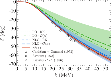
Figure 4: S-wave $p$–$d$ quartet channel scattering phase shifts as functions of the center-of-mass momentum $k$. The curves and bands are as in Fig. 3. Experimental $p$–$d$ phase-shift data are shown from Refs. Arvieux:1973ab (diamonds) and Christian:1953ab (circles). The crosses are the results from the AV18 potential-model calculation reported in Ref. Kievsky:1996ca .

Our result for the scattering length agrees with older experimental determinations Huttel:1983ab ; Arvieux:1973ab but deviates from the more recent determination of Black et al. Black:1999ab and potential-model calculations. At the same time, our results for the phase shifts agree very well with those obtained by Kievsky et al. Kievsky:1996ca in a calculation using the AV18 $NN$ potential (see crosses in Fig. 4). This appears puzzling at first, but it should be noted that the phase shifts at larger momenta are not very sensitive to the Coulomb subtraction and that differences in the scattering length are not visible in Fig. 4 since they are hidden when the cotangent in Eq. (17) is inverted to obtain the low-energy phase shift, which approaches zero as $k\to 0$. In the following, we discuss possible reasons for the discrepancy in the extracted scattering length.

Higher-order electromagnetic effects are not likely to resolve the issue. Diagrams involving the exchange of a transverse photon are suppressed by a factor $\sim Q^{2}/M_{N}^{2}$ compared to the same topology with a Coulomb photon. Since $M_{N}\gg m_{\pi}\sim\Lambda$, such corrections only enter beyond N²LO. A similar argument also holds for magnetic-moment or Mott–Schwinger interactions between the proton and the deuteron. This power counting is supported by the potential model calculation of Kievsky et al. Kievsky:1997jd , which finds only small changes in the scattering length of order $0.05~{}\mathrm{fm}$ when electromagnetic terms beyond the Coulomb interaction are included.

To estimate the effects from the exchange of more than a single Coulomb-photon, we have performed a calculation where the wavy photon line in Figs. 1(a) and (b) is replaced by a photon-mass regulated full Coulomb T-matrix first derived by Gorshkov Gorshkov:1961ab ; Gorshkov:1965ab and further discussed in Refs. Koenig:2013 ; Konig:2014ufa . This calculation is numerically very difficult since the analog of diagram 1(b) involves a four-dimensional numerical integration that we carry out with Monte Carlo techniques. Also, the approach should be taken with a grain of salt since the full T-matrix directly between the deuteron and the proton is only built up perturbatively. Nevertheless, our calculations indicate that this procedure gives values consistent with our result in Eq. (21) within the quoted uncertainty.

Subtraction of Coulomb effects

More likely, the discrepancy is related to the conventional question of how to disentangle short- and long-range Coulomb contributions in the scattering of composite particles. In our effective field theory framework, it is natural to define the pure Coulomb sector by keeping only the diagrams without strong interaction between the proton and the deuteron, i.e., Figs. 1(a) and (c), the latter of which is included perturbatively at higher orders. This is exactly what is stated below Eqs. (19). The leading contribution, Fig. 1(a), contains a nucleon loop that corresponds to the short-range substructure of the deuteron, which is a three-body effect. In configuration-space potential model calculations, on the other hand, the Coulomb subtraction is defined by factorizing the three-body scattering wave function at large distances. If $x$ is the relative coordinate between the two nucleons comprising the deuteron and $y$ is the coordinate of this subsystem relative to the remaining proton, one has (schematically)

$$\psi(x,y)\stackrel{{\scriptstyle y\to\infty}}{{\longrightarrow}}\left[F(\eta,ky)\cot\tilde{\delta}(k)+G(\eta,ky)\right]u(x)\,,$$ (22)

with Coulomb wavefunctions $F(\eta,\rho)$ and $G(\eta,\rho)$. More details can be found, for example, in Ref. Chen:1989zzc . In Eq. (22), we have written $\tilde{\delta}$ instead of $\delta_{\mathrm{diff}}$, since it is not a priori clear to what extent the two quantities are equivalent.

Equation (22) effectively subtracts Coulomb effects purely at the two-body level. Within their respective frameworks, both subtraction methods are completely natural. The question is now whether or not they are equivalent. While one might think that at least in the limit $k\to 0$ the answer would be yes, this does not seem to be the case. The resolution to the discrepancy between our EFT result for the scattering length and those from potential-model calculations would then be that we simply do not calculate the same Coulomb-modified scattering length. In fact, in the above sense it should be appropriate to call the scattering length a (subtraction-)scheme dependent quantity. We stress, however, that this statement is based on one of the particles (the deuteron) being composite. For a two-body system this ambiguity does not occur. Indeed, we have checked the screened momentum-space technique described here with a simple two-body model system. For a spherical step potential, where the Coulomb-subtracted phase shifts can be calculated fully analytically, we find a very good agreement (better than 1%) of our numerical method with the exact result. Thus, in a two-body system our method and Eq. (22) lead to the same answer. In the three-body system, there appears to be a difference related to the short-range three-body Coulomb effects included in the EFT calculation, which introduces a scheme dependence in the Coulomb-subtracted scattering length ${{}^{4}a}_{\text{$p$--$d$}}$.

We emphasize that our diagrammatic subtraction scheme leads to well-defined and numerically stable limits $k\to 0$ and $\lambda\to 0$. In Fig. 5, we show the effective range function—the left-hand side of Eq. (17)—that we obtain at N²LO for momenta $k$ between $2$ and $52~{}\mathrm{MeV}$. It is clear that we can unambiguously extract ${{}^{4}a}_{\text{$p$--$d$}}$ with a weak photon-mass dependence, as shown in Fig. 3.

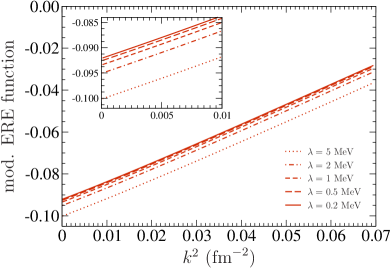
Figure 5: $p$–$d$ effective range function with screened Gamow factor and pure-Coulomb phase shifts from T-matrix based on the EFT calculation. N²LO calculation with cutoff $\Lambda=560~{}\mathrm{MeV}$.

In order to compare the EFT calculation to extractions based on Eq. (22), the question is then to what extent is it possible with our method to obtain ${{}^{4}a}_{\text{$p$--$d$}}$ in the same conventions as in configuration-space potential-model calculations. If the problem is indeed related to the subtraction of short-range three-body effects from the bubble dynamics in Fig. 1(a), we have to find a definition of ${{}^{4}a}_{\text{$p$--$d$}}$ in the EFT which avoids this. One possibility is to treat the pure Coulomb part not within the EFT framework, but to simply calculate the T-matrix for a two-body $p$–$d$ system interacting via a Yukawa potential with mass $\lambda$ (in order to still incorporate the screening effect). With this procedure, $\mathcal{T}_{\mathrm{c}}$ no longer has an EFT expansion but is the same at each order. The same is then true for $\delta_{\mathrm{c}}$ and $C_{\eta,\lambda}^{2}$ (since they are calculated from $\mathcal{T}_{\mathrm{c}}$), so Eq. (20) simplifies quite a bit. We now have

$$\left[k\cot\delta_{\mathrm{diff}}\right]^{(0)} =\frac{2\pi}{\mu}\frac{\mathrm{e}^{2\mathrm{i}\delta_{\mathrm{c}}}}{T_{\mathrm{full}}^{(0)}-T_{\mathrm{c}}}+\mathrm{i}k\,,$$ (23a)

$$\left[k\cot\delta_{\mathrm{diff}}\right]^{(1)} =-\frac{2\pi}{\mu}\mathrm{e}^{2\mathrm{i}\delta_{\mathrm{c}}}\times\left[\frac{T_{\mathrm{full}}^{(1)}}{(T_{\mathrm{full}}^{(0)}-T_{\mathrm{c}})^{2}}\right]\,,$$ (23b)

$$\left[k\cot\delta_{\mathrm{diff}}\right]^{(2)} =-\frac{2\pi}{\mu}\mathrm{e}^{2\mathrm{i}\delta_{\mathrm{c}}}$$ (23c)

$$\hskip 40.00006pt\times\Bigg{[}\frac{T_{\mathrm{full}}^{(2)}}{(T_{\mathrm{full}}^{(0)}-T_{\mathrm{c}})^{2}}-\frac{(T_{\mathrm{full}}^{(1)})^{2}}{(T_{\mathrm{full}}^{(0)}-T_{\mathrm{c}})^{3}}\Bigg{]}\,,$$

reflecting just the perturbative expansion of the full T-matrix $T_{\mathrm{full}}=Z_{0}^{(0)}\mathcal{T}_{\mathrm{full}}^{(0)}+(Z_{0}^{(0)}\mathcal{T}_{\mathrm{full}}^{(1)}+Z_{0}^{(1)}\mathcal{T}_{\mathrm{full}}^{(0)})+\cdots$.

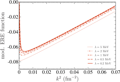
Figure 6: Same as Fig. 5, but now with $\mathcal{T}_{\mathrm{c}}$ calculated from a simple two-body Yukawa potential and for a larger cutoff $\Lambda=56000~{}\mathrm{MeV}$.

The N²LO result for this prescription is shown in Fig. 6 for different values of the Yukawa (photon) mass $\lambda$. At very small $k$, there is now a strong dependence on the photon mass. Keeping in mind that we are no longer subtracting exactly the same Coulomb contributions that enter into the full T-matrix $\mathcal{T}_{\mathrm{full}}$, it may not be surprising that we see problems at very small momenta, where the Coulomb interaction is dominant. On the other hand, one sees that for $k\gtrsim 20~{}\mathrm{MeV}$ the dependence on $\lambda$ is still weak, and in fact the effective range function is quite linear in that regime. Neglecting thus the problems at very small $k$ for the moment, we can extract the scattering length from a fit in the linear regime.

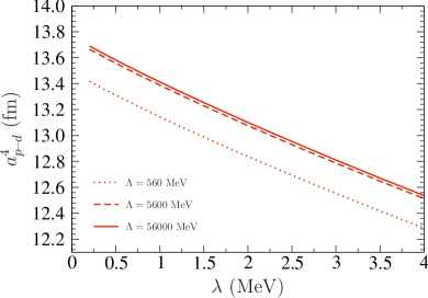
Figure 7: Photon-mass and cutoff dependence of ${{}^{4}a}_{\text{$p$--$d$}}$ with a simple two-body Yukawa subtraction at N²LO in the “$\mathcal{O}(\alpha)$” counting scheme.

The results of this calculation at N²LO (in the “$\mathcal{O}(\alpha)$” counting scheme) are shown in Fig. 7. Overall, this calculation requires somewhat larger cutoffs $\Lambda$ to reach convergence, but the value for ${{}^{4}a}_{\text{$p$--$d$}}$ extracted this way indeed comes out very close to the potential-model results clustered at roughly $13.8~{}\mathrm{fm}$, which lends some support for our explanation of the discrepancy. However, recalling the problems at very small momenta $k$ as well as the rather ad hoc nature of this calculation, this issue requires further study. Here we just note that when we calculate the Coulomb-subtracted phase shifts with the simple Yukawa-subtraction approach, we get a curve at N²LO that lies even closer to the potential-model results shown in Fig. 4. Within the EFT uncertainty, however, the result is equivalent to what we find with the diagrammatic subtraction scheme. This underlines our previous statement that the phase shifts at higher energies are not very sensitive to the details of the Coulomb subtraction.

VI Conclusion and outlook

In this paper, we have presented a new way to extract the $p$–$d$ scattering length from pionless effective field theory calculations. The Coulomb-modified scattering length emerges from the cancellation between $k\cot\delta_{\mathrm{diff}}(k)$ on the one hand, which diverges as $k\to 0$, and the Gamow factor on the other hand, which goes to zero in the same limit. A consistent treatment of screening effects is crucial for a stable and reliable theoretical extraction of this quantity. Our result for the quartet $p$–$d$ scattering length, ${{}^{4}a}_{\text{$p$--$d$}}=(10.9\pm 0.4)~{}\mathrm{fm}$, agrees with older experimental determinations of this quantity but deviates from potential-model calculations and a more recent result from Black et al., which find larger values around $14~{}\mathrm{fm}$ Black:1999ab ; Berthold:1986zz ; Chen:1991zza ; Kievsky:1997jd .

As a possible resolution to this discrepancy, we have investigated the scheme dependence of the Coulomb subtraction in a three-body system. While the Coulomb subtraction in our EFT calculations includes some short-range contributions from the photon coupling to the two-nucleon bubble inside three-body diagrams [cf. Fig. 1(a)], the value for ${{}^{4}a}_{\text{$p$--$d$}}$ extracted from experiments and potential model calculations using Eq. (22) is based on a subtraction of long-range two-body Coulomb effects only. Since both methods lead to the same result in a two-body system, we conjecture that the difference between our results and those of Refs. Black:1999ab ; Berthold:1986zz ; Chen:1991zza ; Kievsky:1997jd is due to short-range three-body Coulomb effects. Moreover, we have illustrated that an approximate (and not fully consistent) implementation of the of the standard Coulomb subtraction leads to larger values of ${{}^{4}a}_{\text{$p$--$d$}}$ in better agreement with Refs. Black:1999ab ; Berthold:1986zz ; Chen:1991zza ; Kievsky:1997jd .

Our findings raise the question of whether the scattering length, being so sensitive to the details of the Coulomb subtraction, is the best quantity to study and whether it might be better to focus on the phase shifts instead, which do not suffer from this problem. It will certainly be interesting to study these matters in more detail. In the future, we plan a more extensive analysis as well as an extension of our calculation to the $p$–$d$ doublet channel.

- (1) T. C. Black, H. J. Karwowski, E. J. Ludwig A. Kievsky, S. Rosati, and M. Viviani, Phys. Lett. B 471 (1999) 103.
- (2) G. H. Berthold and H. Zankel, Phys. Rev. C 34 (1986) 1203.
- (3) C. R. Chen, G. L. Payne, J. L. Friar and B. F. Gibson, Phys. Rev. C 44 (1991) 50.
- (4) A. Kievsky, S. Rosati, M. Viviani, C. R. Brune, H. J. Karwowski, E. J. Ludwig and M. H. Wood, Phys. Lett. B 406 (1997) 292.
- (5) E. Huttel et al., Nucl. Phys. A 406 (1983) 443.
- (6) J. Arvieux, Nucl. Phys. A 221 (1973) 253.
- (7) C. A. Bertulani, H.-W. Hammer, and U. van Kolck, Nucl. Phys. A 712 (2002) 37.
- (8) P. F. Bedaque, H.-W. Hammer, and U. van Kolck, Phys. Lett. B 569 (2003) 159.
- (9) J.-M. Sparenberg, P. Capel, and D. Baye, Phys. Rev. C 81 (2010) 011601.
- (10) S. König, D. Lee and H. -W. Hammer, J. Phys. G: Nucl. Part. Phys. 40 (2013) 045106.
- (11) C.A. Gagliardi et al., Phys. Rev. C 59 (1999) 1149.
- (12) D. B. Kaplan, M. J. Savage and M. B. Wise, Phys. Lett. B 424 (1998) 390.
- (13) U. van Kolck, Nucl. Phys. A 645, (1999) 273.
- (14) H. A. Bethe, Phys. Rev. 76 (1949) 38.
- (15) J. J. de Swart, C. P. F. Terheggen and V. G. J. Stoks, arXiv:nucl-th/9509032.
- (16) P. F. Bedaque and U. van Kolck, Phys. Lett. B 428 (1998) 221.
- (17) P. F. Bedaque, H. W. Hammer and U. van Kolck, Phys. Rev. C 58 (1998) 641.
- (18) X. Kong and F. Ravndal, Phys. Lett. B 450 (1999) 320.
- (19) X. Kong and F. Ravndal, Nucl. Phys. A 665 (2000) 137.
- (20) G. Rupak and X. Kong, Nucl. Phys. A 717 (2003) 73.
- (21) S. Ando and M. C. Birse, J. Phys. G: Nucl. Part. Phys. 37 (2010) 105108.
- (22) S. König and H.-W. Hammer, Phys. Rev. C 83 (2011) 064001.
- (23) C. van der Leun and C. Anderliesten, Nucl. Phys. A 380 (1982) 261.
- (24) P. F. Bedaque, G. Rupak, H. W. Grießhammer and H.-W. Hammer, Nucl. Phys. A 714 (2003) 589.
- (25) J. Vanasse, Phys. Rev. C 88 (2013) 044001.
- (26) S. König, Effective quantum theories with short- and long-range forces, Doctorial thesis (Dissertation), University of Bonn, 2013. http://hss.ulb.uni-bonn.de/2013/3395/3395.htm
- (27) S. König, H. W. Grießhammer and H.-W. Hammer, arXiv:1405.7961 [nucl-th].
- (28) J. Vanasse, D. A. Egolf, J. Kerin, S. König and R. P. Springer, Phys. Rev. C 89 (2014) 064003.
- (29) M. Hoferichter, (private communication, 2010)
- (30) H. van Haeringen and L. P. Kok, Czech. J. Phys. B 32 (1982) 307.
- (31) R. G. Newton, Scattering Theory of Waves and Particles, 2nd edition, Springer-Verlag, New York; Heidelberg; Berlin (1982).
- (32) C. Ji and D. R. Phillips, Few-Body Syst. 54 (2013) 2317.
- (33) H. W. Grießhammer, Nucl. Phys. A 744 (2004) 192.
- (34) R. S. Christian and J. L. Gammel, Phys. Rev. 91 (1953) 100.
- (35) A. Kievsky, S. Rosati, W. Tornow and M. Viviani, Nucl. Phys. A 607 (1996) 402.
- (36) V. G. Gorshkov, Soviet Phys. JETP 13 (1961) 1037.
- (37) V. G. Gorshkov, Soviet Phys. JETP 20 (1965) 234.
- (38) C. R. Chen, G. L. Payne, J. L. Friar and B. F. Gibson, Phys. Rev. C 39 (1989) 1261.