Backing off from Infinity:
Performance Bounds via Concentration of Spectral Measure for Random MIMO Channels

Abstract

The performance analysis of random vector channels, particularly multiple-input-multiple-output (MIMO) channels, has largely been established in the asymptotic regime of large channel dimensions, due to the analytical intractability of characterizing the exact distribution of the objective performance metrics. This paper exposes a new non-asymptotic framework that allows the characterization of many canonical MIMO system performance metrics to within a narrow interval under moderate-to-large channel dimensionality, provided that these metrics can be expressed as a separable function of the singular values of the matrix. The effectiveness of our framework is illustrated through two canonical examples. Specifically, we characterize the mutual information and power offset of random MIMO channels, as well as the minimum mean squared estimation error of MIMO channel inputs from the channel outputs. Our results lead to simple, informative, and reasonably accurate control of various performance metrics in the finite-dimensional regime, as corroborated by the numerical simulations. Our analysis framework is established via the concentration of spectral measure phenomenon for random matrices uncovered by Guionnet and Zeitouni, which arises in a variety of random matrix ensembles irrespective of the precise distributions of the matrix entries.

I Introduction

The past decade has witnessed an explosion of developments in multi-dimensional vector channels [1], particularly multiple-input-multiple-output (MIMO) channels. The exploitation of multiple (possibly correlated) dimensions provides various benefits in wireless communication and signal processing systems, including channel capacity gain, improved energy efficiency, and enhanced robustness against noise and channel variation.

Although many fundamental MIMO system performance metrics can be evaluated via the precise spectral distributions of finite-dimensional MIMO channels (e.g. channel capacity [2, 3], minimum mean square error (MMSE) estimates of vector channel inputs from the channel outputs [4], power offset [5], sampled capacity loss [6]), this approach often results in prohibitive analytical and computational complexity in characterizing the probability distributions and confidence intervals of these MIMO system metrics. In order to obtain more informative analytical insights into the MIMO system performance metrics, a large number of works (e.g. [7, 8, 9, 10, 11, 5, 12, 13, 14, 15, 16, 17, 18, 19, 20, 21]) present more explicit expressions for these performance metrics with the aid of random matrix theory. Interestingly, when the number of input and output dimensions grow, many of the MIMO system metrics taking the form of linear spectral statistics converge to deterministic limits, due to various limiting laws and universality properties of (asymptotically) large random matrices [22]. In fact, the spectrum (i.e. singular-value distribution) of a random channel matrix $\boldsymbol{H}$ tends to stabilize when the channel dimension grows, and the limiting distribution is often universal in the sense that it is independent of the precise distributions of the entries of $\boldsymbol{H}$.

These asymptotic results are well suited for massive MIMO communication systems. However, the limiting regime falls short in providing a full picture of the phenomena arising in most practical systems which, in general, have moderate dimensionality. While the asymptotic convergence rates of many canonical MIMO system performance metrics have been investigated as well, how large the channel dimension must be largely depends on the realization of the growing matrix sequences. In this paper, we propose an alternative method via concentration of measure to evaluate many canonical MIMO system performance metrics for finite-dimension channels, assuming that the target performance metrics can be transformed into linear spectral statistics of the MIMO channel matrix. Moreover, we show that the metrics fall within narrow intervals with high (or even overwhelming) probability for moderate-to-high dimensional channels.

I-A Related Work

Random matrix theory is one of the central topics in probability theory with many connections to wireless communications and signal processing. Several random matrix ensembles, such as Gaussian unitary ensembles, admit exact characterization of their eigenvalue distributions [23] under any channel dimensionality. These spectral distributions associated with the finite-dimensional MIMO channels can then be used to compute analytically the distributions and confidence intervals of the MIMO system performance metrics (e.g. mutual information of MIMO fading channels [24, 25, 26, 27, 28]). However, the computational intractability of integrating a large-dimensional function over a finite-dimensional MIMO spectral distribution precludes concise and informative capacity expressions even in moderate-sized problems. For this reason, theoretical analysis based on precise eigenvalue characterization is generally limited to small-dimensional vector channels.

In comparison, one of the central topics in modern random matrix theory is to derive limiting distributions for the eigenvalues of random matrix ensembles of interest, which often turns out to be simple and informative. Several pertinent examples include the semi-circle law for symmetric Wigner matrices [29], the circular law for i.i.d. matrix ensembles [30, 31], and the Marchenko–Pastur law [32] for rectangular random matrices. One remarkable feature of these asymptotic laws is the universality phenomenon, whereby the limiting spectral distributions are often indifferent to the precise distribution of each matrix entry. This phenomenon allows theoretical analysis to accommodate a broad class of random matrix families beyond Gaussian ensembles. See [22] for a beautiful and self-contained exposition of these limiting results.

The simplicity and universality of these asymptotic laws have inspired a large body of work in characterizing the asymptotic performance limits of random vector channels. For instance, the limiting results for i.i.d. Gaussian ensembles have been applied in early work [2] to establish the linear increase of MIMO capacity with the number of antennas. This approach was then extended to accommodate separable correlation fading models [8, 12, 14, 16, 15, 33, 34] with general non-Gaussian distributions (particularly Rayleigh and Ricean fading [13, 5]). These models admit analytically-friendly solutions, and have become the cornerstone for many results for random MIMO channels. In addition, several works have characterized the second-order asymptotics (often in the form of central limit theorems) for mutual information [16, 35, 36], information density [37], second-order coding rates [38, 39], diversity-multiplexing tradeoff [40], etc., which uncover the asymptotic convergence rates of various MIMO system performance metrics under a large family of random matrix ensembles. The limiting tail of the distribution (or large deviation) of the mutual information has also been determined in the asymptotic regime [41]. In addition to information theoretic metrics, other signal processing and statistical metrics like MMSE [7, 42, 43], multiuser efficiency for CDMA systems [10], optical capacity [44], covariance matrix and principal components [45], canonical correlations [46], and likelihood ratio test statistics [46], have also been investigated via asymptotic random matrix theory. While these asymptotic laws have been primarily applied to performance metrics in the form of linear spectral statistics, more general performance metrics can be approximated using the delicate method of “deterministic equivalents” (e.g. [47, 48]).

A recent trend in statistics is to move from asymptotic laws towards non-asymptotic analysis of random matrices [49, 50], which aims at revealing statistical effects of a moderate-to-large number of components, assuming a sufficient amount of independence among them. One prominent effect in this context is the concentration of spectral measure phenomenon [51, 52], which indicates that many separable functions of a matrix’s singular values (called linear spectral statistics [53]) can be shown to fall within a narrow interval with high probability even in the moderate-dimensional regime. This phenomenon has been investigated in various fields such as high-dimensional statistics [49], statistical learning [54], and compressed sensing [50].

Inspired by the success of the measure concentration methods in the statistics literature, our recent work [6] develops a non-asymptotic approach to quantify the capacity of multi-band channels under random sub-sampling strategies, which to our knowledge is the first to exploit the concentration of spectral measure phenomenon to analyze random MIMO channels. In general, the concentration of measure phenomena are much less widely recognized and used in the communication community than in the statistics and signal processing community. Recent emergence of massive MIMO technologies [55, 56, 57, 58], which uses a large number of antennas to obtain both capacity gain and improved radiated energy efficiency, provides a compelling application of these methods to characterize system performance. Other network / distributed MIMO systems (e.g. [59, 60]) also require analyzing large-dimensional random vector channels. It is our aim here to develop a general framework that promises new insights into the performance of these emerging technologies under moderate-to-large channel dimensionality.

I-B Contributions

We develop a general non-asymptotic framework for deriving performance bounds of random vector channels or any general MIMO system, based on the powerful concentration of spectral measure phenomenon of random matrices as revealed by Guionnet and Zeitouni [51]. Specifically, we introduce a general recipe that can be used to assess various MIMO system performance metrics to within vanishingly small confidence intervals, assuming that the objective metrics can be transformed into linear spectral statistics associated with the MIMO channel. Our framework and associated results can accommodate a large class of probability distributions for random channel matrices, including those with bounded support, a large class of sub-Gaussian measures, and heavy-tailed distributions. To broaden the range of metrics that we can accurately evaluate, we also develop a general concentration of spectral measure inequality for the cases where only the exponential mean (instead of the mean) of the objective metrics can be computed.

We demonstrate the effectiveness of our approach through two illustrative examples: (1) mutual information of random vector channels under equal power allocation; (2) MMSE in estimating signals transmitted over random MIMO channels. These examples allow concise and, informative characterizations even in the presence of moderate-to-high SNR and moderate-to-large channel dimensionality. In contrast to a large body of prior works that focus on first-order limits or asymptotic convergence rate of the target performance metrics, we are able to derive full characterization of these metrics in the non-asymptotic regime. Specifically, we obtain narrow confidence intervals with precise order and reasonably accurate pre-constants, which do not rely on careful choice of the growing matrix sequence. Our numerical simulations also corroborate that our theoretical predictions are reasonably accurate in the finite-dimensional regime.

I-C Organization and Notation

The rest of the paper is organized as follows. Section II introduces several families of probability measures investigated in this paper. We present a general framework characterizing the concentration of spectral measure phenomenon in Section III. In Section IV, we illustrate the general framework using a small sample of canonical examples. Finally, Section V concludes the paper with a summary of our findings and a discussion of several future directions.

For convenience of presentation, we let $\mathbb{C}$ denote the set of complex numbers. For any function $g(x)$, the Lipschitz norm of $g(\cdot)$ is defined as

$$\left\|g\right\|_{\mathcal{L}}:=\sup_{x\neq y}\left|\frac{g\left(x\right)-g\left(y\right)}{x-y}\right|.$$ (1)

We let $\lambda_{i}(\boldsymbol{A})$, $\lambda_{\max}(\boldsymbol{A})$, and $\lambda_{\min}(\boldsymbol{A})$ represent the $i$th largest eigenvalue, the largest eigenvalue, and the smallest eigenvalue of a Hermitian matrix $\boldsymbol{A}$, respectively, and use $\left\|\cdot\right\|$ to denote the operator norm (or spectral norm). The set $\left\{1,2,\cdots,n\right\}$ is denoted as $[n]$, and we write ${[n]\choose k}$ for the set of all $k$-element subsets of $[n]$. For any set $\boldsymbol{s}$, we use $\mathrm{card}(\boldsymbol{s})$ to represent the cardinality of $\boldsymbol{s}$. Also, for any two index sets $\boldsymbol{s}$ and $\boldsymbol{t}$, we denote by $\boldsymbol{A}_{\boldsymbol{s},\boldsymbol{t}}$ the submatrix of $\boldsymbol{A}$ containing the rows at indices in $\boldsymbol{s}$ and columns at indices in $\boldsymbol{t}$. We use $x\in a+[b,c]$ to indicate that $x$ lies within the interval $[a+b,a+c]$. Finally, the standard notation $f(n)=\mathcal{O}\left(g(n)\right)$ means that there exists a constant $c>0$ such that $f(n)\leq cg(n)$; $f(n)=\Theta\left(g(n)\right)$ indicates that there are universal constants $c_{1},c_{2}>0$ such that $c_{1}g(n)\leq f(n)\leq c_{2}g(n)$; and $f(n)=\Omega\left(g(n)\right)$ indicates that there are universal constants $c>0$ such that $f(n)\leq cg(n)$. Throughout this paper, we use $\log\left(\cdot\right)$ to represent the natural logarithm. Our notation is summarized in Table I.

Table I: Summary of Notation and Parameters

$\log(\cdot)$	natural logarithm
$\kappa$	$\kappa=1$ for the real-valued case and $\kappa=2$ for the complex-valued case
$\nu_{ij},\nu$	the standard deviation of $\boldsymbol{M}_{ij}$, and the maximum standard deviation $\nu:=\max_{i,j}\nu_{ij}$
$c_{\mathrm{ls}}$	logarithmic Sobolev constant as defined in (3)
$\left\|\cdot\right\|_{\mathcal{L}}$	Lipschitz constant of a function
$D$	maximum absolute value in the compact support of a bounded measure
$\tau_{c}$, $\sigma_{c}$	truncation threshold and the associated standard deviation defined in (7) and (8), respectively
$\rho$	spectral radius of the deterministic matrix $\boldsymbol{R}$
$[n]$	$[n]:=\left\{1,2,\cdots,n\right\}$
${[n]\choose k}$	set of all $k$-element subsets of $[n]$

II Three Families of Probability Measures

In this section, we define precisely three classes of probability measures with different properties of the tails, which lay the foundation of the analysis in this paper.

Definition 1 (Bounded Distribution).

We say that a random variable $X\in\mathbb{C}$ is bounded by $D$ if

$$\mathbb{P}\left(\left|X\right|\leq D\right)=1.$$ (2)

The class of probability distributions that have bounded support subsumes as special cases a broad class of distributions encountered in practice (e.g. the Bernoulli distribution and uniform distribution). Another class of probability measures that possess light tails (i.e. sub-Gaussian tails) is defined as follows.

Definition 2 (Logarithmic Sobolev Measure).

We say that a random variable $X\in\mathbb{C}$ with cumulative probability distribution (CDF) $F\left(\cdot\right)$ satisfies the logarithmic Sobolev inequality (LSI) with uniform constant $c_{\mathrm{ls}}$ if, for any differentiable function $h$, one has

$${\displaystyle\int}h^{2}(x)\log\left(\frac{h^{2}(x)}{\int h^{2}(z)\mathrm{d}F(z)}\right)\mathrm{d}F(x)\leq 2c_{\mathrm{ls}}\int\left|h^{\prime}(x)\right|^{2}\mathrm{d}F(x).$$ (3)

Remark 1.

One of the most popular techniques in demonstrating measure concentration is the “entropy method” (see, e.g. [61, 62]), which hinges upon establishing inequalities of the form

$$\mathrm{KL}\left(\mathbb{P}_{X}^{t}\|\mathbb{P}_{X}\right)\leq O\left(t^{2}\right)$$ (4)

for some measure $\mathbb{P}_{X}$ and its tilted measure $\mathbb{P}_{X}^{t}$, where $\mathrm{KL}\left(\cdot\|\cdot\right)$ denotes the Kullback–Leibler divergence. See [62, Chapter 3] for detailed definitions and derivation. It turns out that for a probability measure satisfying the LSI, one can pick the function $h(\cdot)$ in (3) in some appropriate fashion to yield the entropy-type inequality (4). In fact, the LSI has been well recognized as one of the most fundamental criteria to demonstrate exponentially sharp concentration for various metrics.

Remark 2.

While the measure satisfying the LSI necessarily exhibits sub-Gaussian tails (e.g. [61, 62]), many concentration results under log-Sobolev measures cannot be extended to general sub-Gaussian distributions (e.g. for bounded measures the concentration results have only been shown for convex functions instead of general Lipschitz functions).

A number of measures satisfying the LSI have been discussed in the expository paper [63]. One of the most important examples is the standard Gaussian distribution, which satisfies the LSI with logarithmic Sobolev constant $c_{\mathrm{LS}}=1$. In many situations, the probability measures obeying the LSI exhibit very sharp concentration of spectral measure phenomenon (typically sharper than general bounded measures).

While prior works on measure concentration focus primarily on measures with bounded support or measures with sub-Gaussian tails, it is also of interest to accommodate a more general class of distributions (e.g. heavy-tailed distributions). For this purpose, we introduce sub-exponential distributions and heavy-tailed distributions as follows.

Definition 3 (Sub-Exponential Distribution).

A random variable $X$ is said to be sub-exponentially distributed with parameter $\lambda$ if it satisfies

$$\mathbb{P}\left(\left|X\right|>x\right)\leq c_{0}e^{-\lambda x},\quad\forall x>0$$ (5)

for some absolute constant $c_{0}>0$.

Definition 4 (Heavy-tailed Distribution).

A random variable $X$ is said to be heavy-tailed distributed if

$$\lim_{x\rightarrow\infty}e^{-\lambda x}\mathbb{P}\left(\left|X\right|>x\right)=\infty,\quad\forall\lambda>0.$$ (6)

That said, sub-exponential (resp. heavy-tailed) distributions are those probability measures whose tails are lighter (resp. heavier) than exponential distributions. Commonly encountered heavy-tailed distributions include log-normal and power-law distributions.

To facilitate analysis, for both sub-exponential and heavy-tailed distributions, we define the following two quantities $\tau_{c}$ and $\sigma_{c}$ with respect to $X$ for some sequence $c(n)$ such that

$$\mathbb{P}\left(\left|X\right|>\tau_{c}\right)\leq\frac{1}{mn^{c(n)+1}},$$ (7)

and

$$\sigma_{c}=\sqrt{\mathbb{E}\left[\left|X\right|^{2}{\bf 1}{}_{\left\{\left|X\right|<\tau_{c}\right\}}\right]}.$$ (8)

In short, $\tau_{c}$ represents a truncation threshold such that the truncated $X$ coincides with the true $X$ with high probability, and $\sigma_{c}$ denotes the standard deviation of the truncated $X$. The idea is to study $X{\bf 1}{}_{\left\{\left|X\right|<\tau_{c}\right\}}$ instead of $X$ in the analysis, since the truncated value is bounded and exhibits light tails. For instance, if $X$ is exponentially distributed such that $\mathbb{P}\left(\left|X\right|>x\right)=e^{-x}$ and $c(n)=\log n$, then this yields that

$$\tau_{c}=\log^{2}n+\log\left(mn\right).$$

Typically, one would like to pick $c(n)$ such that $\tau_{c}$ becomes a small function of $m$ and $n$ obeying $\sigma_{c}^{2}\approx\mathbb{E}[\left|X\right|^{2}]$.

III Concentration of Spectral Measure in Large Random Vector Channels

We present a general mathematical framework that facilitates the analysis of random vector channels. The proposed approach is established upon the concentration of spectral measure phenomenon derived by Guionnet and Zeitouni [51], which is a consequence of Talagrand’s concentration inequalities [64]. While the adaptation of such general concentration results to our settings requires moderate mathematical effort, it leads to a very effective framework to assess the fluctuation of various MIMO system performance metrics. We will provide a few canonical examples in Section IV to illustrate the power of this framework.

Consider a random matrix $\boldsymbol{M}=[\boldsymbol{M}_{ij}]_{1\leq i\leq n,1\leq j\leq m}$, where $\boldsymbol{M}_{ij}$’s are assumed to be independently distributed. We use $\boldsymbol{M}_{ij}^{\mathrm{R}}$ and $\boldsymbol{M}_{ij}^{\mathrm{I}}$ to represent respectively the real and imaginary parts of $\boldsymbol{M}_{ij}$, which are also generated independently. Note, however, that $\boldsymbol{M}_{ij}$’s are not necessarily drawn from identical distributions. Set the numerical value

$$\kappa:=\begin{cases}1,\quad&\text{in the real-valued case},\\ 2,\quad&\text{in the complex-valued case}.\end{cases}$$ (9)

We further assume that all entries have matching two moments such that for all $i$ and $j$:

$$\quad\quad\mathbb{E}\left[\boldsymbol{M}_{ij}\right]=0,\quad\quad\quad{\bf Var}\left(\boldsymbol{M}_{ij}^{\mathrm{R}}\right)=\nu_{ij}^{2},$$ (10)

$${\bf Var}\left(\boldsymbol{M}_{ij}^{\mathrm{I}}\right)=\begin{cases}\nu_{ij}^{2},\quad&\text{in the complex-valued case},\\ 0,&\text{in the real-valued case},\end{cases}$$ (11)

where $\nu_{ij}^{2}$ ($\nu_{ij}\geq 0$) are uniformly bounded by

$$\max_{i,j}\left|\nu_{ij}\right|\leq\nu.$$ (12)

In this paper, we focus on the class of MIMO system performance metrics that can be transformed into additively separable functions of the eigenvalues of the random channel matrix (called linear spectral statistics [53]), i.e. the type of metrics taking the form

$$\sum_{i=1}^{n}f\left(\lambda_{i}\left(\frac{1}{n}\boldsymbol{M}\boldsymbol{R}\boldsymbol{R}^{*}\boldsymbol{M}^{*}\right)\right)$$ (13)

for some function $f\left(\cdot\right)$ and some deterministic matrix $\boldsymbol{R}\in\mathbb{C}^{m\times m}$, where $\lambda_{i}\left(\boldsymbol{X}\right)$ denotes the $i$th eigenvalue of a matrix $\boldsymbol{X}$. As can been seen, many vector channel performance metrics (e.g. MIMO mutual information, MMSE, sampled channel capacity loss) can all be transformed into certain forms of linear spectral statistics. We will characterize in Proposition 1 and Theorem 1 the measure concentration of (13), which quantifies the fluctuation of (13) in finite-dimensional random vector channels.

III-A Concentration Inequalities for the Spectral Measure

Many linear spectral statistics of random matrices sharply concentrate within a narrow interval indifferent to the precise entry distributions. Somewhat surprisingly, such spectral measure concentration is shared by a very large class of random matrix ensembles. We provide formal quantitative illustration of such concentration of spectral measure phenomena below, which follows from [51, Corollary 1.8]. This behavior, while not widely used in communication and signal processing, is a general result in probability theory derived from the Talagrand concentration inequality (see [64] for details).

Before proceeding to the concentration results, we define

$$f_{0}\left(\boldsymbol{M}\right):=\frac{1}{n}\sum_{i=1}^{\min\left(m,n\right)}f\left(\lambda_{i}\left(\frac{1}{n}\boldsymbol{M}\boldsymbol{R}\boldsymbol{R}^{*}\boldsymbol{M}^{*}\right)\right)$$ (14)

for the sake of notational simplicity.

Proposition 1.

Consider a random matrix $\boldsymbol{M}=\left[\boldsymbol{M}_{ij}\right]_{1\leq i\leq n,1\leq j\leq m}$ satisfying (10) and (12). Suppose that $\boldsymbol{R}\in\mathbb{C}^{m\times m}$ is any given matrix and $\left\|\boldsymbol{R}\right\|\leq\rho.$ Consider a function $f(x)$ such that $g(x):=f\left(x^{2}\right)$ ($x\in\mathbb{R}^{+}$) is a real-valued Lipschitz function with Lipschitz constant $\left\|g\right\|_{\mathcal{L}}$ as defined in (1). Let $\kappa$ and $\nu$ be defined in (9) and (12), respectively.

(a) (Bounded Measure) If $\boldsymbol{M}_{ij}$’s are bounded by $D$ and $g(\cdot)$ is convex, then for any $\beta>8\sqrt{\pi}$,

$$\left|f_{0}\left(\boldsymbol{M}\right)-\mathbb{E}\left[f_{0}\left(\boldsymbol{M}\right)\right]\right|\leq\frac{\beta D\rho\nu\left\|g\right\|_{\mathcal{L}}}{n}$$ (15)

with probability exceeding $1-4\exp\left(-\frac{\beta^{2}}{8\kappa}\right)$.

(b) (Logarithmic Sobolev Measure) If the measure of $\boldsymbol{M}_{ij}$ satisfies the LSI with a uniformly bounded constant $c_{\mathrm{ls}}$, then for any $\beta>0,$

$$\left|f_{0}\left(\boldsymbol{M}\right)-\mathbb{E}\left[f_{0}\left(\boldsymbol{M}\right)\right]\right|\leq\frac{\beta\sqrt{c_{\mathrm{ls}}}\rho\nu\left\|g\right\|_{\mathcal{L}}}{n}$$ (16)

with probability exceeding $1-2\exp\left(-\frac{\beta^{2}}{\kappa}\right)$.

(c) (Sub-Exponential and Heavy-tailed Measure) Suppose that $\boldsymbol{M}_{ij}$’s are independently drawn from either sub-exponential distributions or heavy-tailed distributions and that their distributions are symmetric about 0, with $\tau_{c}$ and $\sigma_{c}$ defined respectively in (7) and (8) with respect to $\boldsymbol{M}_{ij}$ for some sequence $c(n)$. If $g(\cdot)$ is convex, then

$$\left|f_{0}\left(\boldsymbol{M}\right)-\mathbb{E}\left[f_{0}\left(\tilde{\boldsymbol{M}}\right)\right]\right|\leq\frac{2\kappa\sqrt{c(n)\log n}\tau_{c}\sigma_{c}\rho\left\|g\right\|_{\mathcal{L}}}{n}$$ (17)

with probability exceeding $1-5n^{-c(n)}$, where $\tilde{\boldsymbol{M}}$ is defined such that $\tilde{\boldsymbol{M}}_{ij}:=\boldsymbol{M}_{ij}{\bf 1}{}_{\left\{\left|\boldsymbol{M}_{ij}\right|<\tau_{c}\right\}}$.

Proof.

See Appendix A.∎

Remark 3.

By setting $\beta=\sqrt{\log n}$ in Proposition 1(a) and (b), one can see that under either measures of bounded support or measures obeying the LSI,

$$\left|f_{0}\left(\boldsymbol{M}\right)-\mathbb{E}\left[f_{0}\left(\tilde{\boldsymbol{M}}\right)\right]\right|=\mathcal{O}\left(\frac{\sqrt{\log n}}{n}\right)$$ (18)

with high probability. In contrast, under heavy-tailed measures,

$$\left|f_{0}\left(\boldsymbol{M}\right)-\mathbb{E}\left[f_{0}\left(\tilde{\boldsymbol{M}}\right)\right]\right|=\mathcal{O}\left(\frac{\sqrt{c(n)\tau_{c}^{2}\sigma_{c}^{2}\log n}}{n}\right)$$ (19)

with high probability, where $\sqrt{c(n)}\tau_{c}\sigma_{c}$ is typically a growing function in $n$. As a result, the concentration under sub-Gaussian distributions is sharper than that under heavy-tailed measures by a factor of $\sqrt{c(n)}\tau_{c}\sigma_{c}$.

Remark 4.

The bounds derived in Proposition 1 scale linearly with $\nu$, which is the maximum standard deviation of the entries of $\boldsymbol{M}$. This allows us to assess the concentration phenomena for matrices with entries that have non-uniform variance.

Proposition 1(a) and 1(b) assert that for both measures of bounded support and a large class of sub-Gaussian distributions, many separable functions of the spectra of random matrices exhibit sharp concentration, assuming a sufficient amount of independence between the entries. More remarkably, the tails behave at worst like a Gaussian random variable with well-controlled variance. Note that for a bounded measure, we require the objective metric of the form (13) to satisfy certain convexity conditions in order to guarantee concentration. In contrast, the fluctuation of general Lipschitz functions can be well controlled for logarithmic Sobolev measures. This agrees with the prevailing wisdom that the standard Gaussian measure (which satisfies the LSI) often exhibits sharper concentration than general bounded distributions (e.g. Bernoulli measures).

Proposition 1(c) demonstrates that spectral measure concentration arises even when the tail distributions of $\boldsymbol{M}_{ij}$ are much heavier than standard Gaussian random variables, although it might not be as sharp as for sub-Gaussian measures. This remarkable feature comes at a price, namely, the deviation of the objective metrics is much less controlled than for sub-Gaussian distributions. However, this degree of concentration might still suffice for most practical purposes. Note that the concentration result for heavy-tailed distributions is stated in terms of the truncated version $\tilde{\boldsymbol{M}}$. The nice feature of the truncated $\tilde{\boldsymbol{M}}$ is that its entries are all bounded (and hence sub-Gaussian), which can often be quantified or estimated in a more convenient fashion. Finally, we remark that the concentration depends on the choice of the sequence $c(n)$, which in turn affects the size of $\tau_{c}$ and $\sigma_{c}$. We will illustrate the resulting size of confidence intervals in Section III-C via several examples.

III-B Approximation of Expected Empirical Distribution

Although Proposition 1 ensures sharp measure concentration of various linear spectral statistics, a more precise characterization requires evaluating the mean value of the target metric (13) (i.e. $\mathbb{E}\left[f_{0}\left(\boldsymbol{M}\right)\right]$). While limiting laws often admit simple asymptotic characterization of this mean value for a general class of metrics, whether the convergence rate can be quantified often needs to be studied on a case-by-case basis. In fact, this has become an extensively researched topic in mathematics (e.g. [65, 66, 67, 68]). In this subsection, we develop an approximation result that allows the expected value of a broader class of metrics to be well approximated by concise and informative expressions.

Recall that

$$f_{0}\left(\boldsymbol{M}\right):=\frac{1}{n}\sum_{i=1}^{\min\left(m,n\right)}f\left(\lambda_{i}\left(\frac{1}{n}\boldsymbol{M}\boldsymbol{R}\boldsymbol{R}^{*}\boldsymbol{M}^{*}\right)\right)$$ (20)

We consider a large class of situations where the exponential mean of the target metric (13)

$$\mathcal{E}\left(f\right): =\mathbb{E}\left[\exp\left(nf_{0}\left(\boldsymbol{M}\right)\right)\right]$$ (21)

$$=\mathbb{E}\left[\exp\left(\sum_{i=1}^{\min\{m,n\}}f\left(\lambda_{i}\left(\frac{1}{n}\boldsymbol{M}\boldsymbol{R}\boldsymbol{R}^{*}\boldsymbol{M}^{*}\right)\right)\right)\right]$$

(instead of $\mathbb{E}\left[f_{0}\left(\boldsymbol{M}\right)\right]$) can be approximated in a reasonably accurate manner. This is particularly relevant when $f(\cdot)$ is a logarithmic function. For example, this applies to log-determinant functions

$$f_{0}\left(\boldsymbol{M}\right)=\frac{1}{n}\log\mathrm{\det}\left(\boldsymbol{I}+\frac{1}{n}\boldsymbol{M}\boldsymbol{R}\boldsymbol{R}^{*}\boldsymbol{M}^{*}\right),$$

which are of significant interest in various applications such as wireless communications [69], multivariate hypothesis testing [70], etc. While $\mathbb{E}\left[\mathrm{\det}\left(\boldsymbol{I}+\frac{1}{n}\boldsymbol{M}\boldsymbol{M}^{*}\right)\right]$ often admits a simple distribution-free expression, $\mathbb{E}\left[\log\mathrm{\det}\left(\boldsymbol{I}+\frac{1}{n}\boldsymbol{M}\boldsymbol{M}^{*}\right)\right]$ is highly dependent on precise distributions of the entries of the matrix.

One might already notice that, by Jensen’s inequality, $\log\mathcal{E}\left(f\right)$ is larger than the mean objective metric $\mathbb{E}\left[f_{0}\left(\boldsymbol{M}\right)\right]$. Nevertheless, in many situations, these two quantities differ by only a vanishingly small gap, which is formally demonstrated in the following lemma.

Lemma 1.

(a) (Sub-Exponential Tail) Suppose that

$$\mathbb{P}\left(\left|f_{0}\left(\boldsymbol{M}\right)-\mathbb{E}\left[f_{0}\left(\boldsymbol{M}\right)\right]\right|>\frac{y}{n}\right)\leq c_{1}\exp\left(-c_{2}y\right)$$

for some values $c_{1}>0$ and $c_{2}>1$, then

$$\frac{1}{n}\log\mathcal{E}\left(f\right)-\frac{\log\left(1+\frac{c_{1}}{c_{2}-1}\right)}{n}\leq\mathbb{E}\left[f_{0}\left(\boldsymbol{M}\right)\right]\leq\frac{1}{n}\log\mathcal{E}\left(f\right)$$ (22)

with $\mathcal{E}\left(f\right)$ defined in (21).

(b) (Sub-Gaussian Tail) Suppose that

$$\mathbb{P}\left(\left|f_{0}\left(\boldsymbol{M}\right)-\mathbb{E}\left[f_{0}\left(\boldsymbol{M}\right)\right]\right|>\frac{y}{n}\right)\leq c_{1}\exp\left(-c_{2}y^{2}\right)$$

for some values $c_{1}>0$ and $c_{2}>0$, then

$$\frac{1}{n}\log\mathcal{E}\left(f\right) \geq\mathbb{E}\left[f_{0}\left(\boldsymbol{M}\right)\right]$$

$$\geq\frac{1}{n}\log\mathcal{E}\left(f\right)-\frac{\small\log\small\left(1+\sqrt{\frac{\pi c_{1}^{2}}{c_{2}}}\exp\left(\frac{1}{4c_{2}}\right)\right)}{n}$$ (23)

with $\mathcal{E}\left(f\right)$ defined in (21).

Proof.

See Appendix B.∎

Remark 5.

For measures with sub-exponential tails, if $c_{2}<1$, the concentration is not decaying sufficiently fast and is unable to ensure that $\mathcal{E}\left(f\right)=\mathbb{E}\left[e^{nf_{0}\left(\boldsymbol{M}\right)}\right]$ exists.

In short, Lemma 1 asserts that if $f_{0}\left(\boldsymbol{M}\right)$ possesses a sub-exponential or a sub-Gaussian tail, then $\mathbb{E}[f_{0}\left(\boldsymbol{M}\right)]$ can be approximated by $\frac{1}{n}\log\mathcal{E}\left(f\right)$ in a reasonably tight manner, namely, within a gap no worse than $\mathcal{O}\left(\frac{1}{n}\right)$. Since Proposition 1 implies sub-Gaussian tails for various measures, we immediately arrive at the following concentration results that concern a large class of sub-Gaussian and heavy-tailed measures.

Theorem 1.

Let $c_{\rho,f,D}$, $c_{\rho,f,c_{\mathrm{ls}}}$, and $c_{\rho,f,\tau_{c},\sigma_{c}}$ be numerical values defined in Table II, and set

$$\mu_{\rho,g,A}:=\nu\rho\left\|g\right\|_{\mathcal{L}}A.$$ (24)

(1) (Bounded Measure) Under the assumptions of Proposition 1(a), we have

$$\begin{cases}f_{0}\left(\boldsymbol{M}\right)&\leq\frac{1}{n}\log\mathcal{E}\left(f\right)+\frac{\beta\mu_{\rho,g,D}}{n},\\ f_{0}\left(\boldsymbol{M}\right)&\geq\frac{1}{n}\log\mathcal{E}\left(f\right)-\frac{\beta\mu_{\rho,g,D}}{n}-\frac{c_{\rho,f,D}}{n},\end{cases}$$ (25)

with probability exceeding $1-4\exp\left(-\frac{\beta^{2}}{8\kappa}\right)$.

(2) (Logarithmic Sobolev Measure) Under the assumptions of Proposition 1(b), we have

$$\begin{cases}f_{0}\left(\boldsymbol{M}\right)&\leq\frac{1}{n}\log\mathcal{E}\left(f\right)+\frac{\beta\mu_{\rho,g,\sqrt{c_{\mathrm{ls}}}}}{n},\\ f_{0}\left(\boldsymbol{M}\right)&\geq\frac{1}{n}\log\mathcal{E}\left(f\right)-\frac{\beta\mu_{\rho,g,\sqrt{c_{\mathrm{ls}}}}}{n}-\frac{c_{\rho,f,c_{\mathrm{ls}}}}{n},\end{cases}$$ (26)

with probability at least $1-2\exp\left(-\frac{\beta^{2}}{\kappa}\right)$.

(3) (Heavy-tailed Distribution) Under the assumptions of Proposition 1(c), we have

$$\begin{cases}f_{0}\left(\boldsymbol{M}\right)&\leq\frac{1}{n}\log\mathcal{E}_{\tilde{\boldsymbol{M}}}\left(f\right)+\frac{\mu_{\rho,g,\zeta}}{n},\\ f_{0}\left(\boldsymbol{M}\right)&\geq\frac{1}{n}\log\mathcal{E}_{\tilde{\boldsymbol{M}}}\left(f\right)-\frac{\mu_{\rho,g,\zeta}}{n}-\frac{c_{\rho,f,\tau_{c},\sigma_{c}}}{n},\end{cases}$$ (27)

with probability exceeding $1-5n^{-c(n)}$, where

$$\begin{cases}\zeta&:=\text{ }\tau_{c}\sigma_{c}\sqrt{8\kappa c(n)\log n};\\ \mathcal{E}_{\tilde{\boldsymbol{M}}}\left(f\right)&:=\text{ }\mathbb{E}\left[\exp\left(nf_{0}\left(\tilde{\boldsymbol{M}}\right)\right)\right].\end{cases}$$

Proof.

See Appendix C.∎

Table II: Summary of parameters of Theorem 1.

$c_{\rho,f,D}:=\log\left(1+\sqrt{8\kappa\pi}D\rho\nu\left\|g\right\|_{\mathcal{L}}e^{\frac{8\pi}{\kappa}+2\kappa D^{2}\rho^{2}\nu^{2}\left\|g\right\|_{\mathcal{L}}^{2}}\right)$

$c_{\rho,f,c_{\mathrm{ls}}}:=\log\left(1+\sqrt{4\kappa\pi c_{\mathrm{ls}}}\rho\nu\left\|g\right\|_{\mathcal{L}}e^{\frac{\kappa}{4}c_{\mathrm{ls}}\rho^{2}\nu^{2}\left\|g\right\|_{\mathcal{L}}^{2}}\right)$

$c_{\rho,f,\tau_{c},\sigma_{c}}:=\log\left(1+\sqrt{8\kappa\pi}\tau_{c}\sigma_{c}\rho\left\|g\right\|_{\mathcal{L}}e^{\frac{8\pi}{\kappa}+2\kappa\tau_{c}^{2}\sigma_{c}^{2}\rho^{2}\left\|g\right\|_{\mathcal{L}}^{2}}\right)$

While Lemma 1 focuses on sub-exponential and sub-Gaussian measures, we are able to extend the concentration phenomenon around $\frac{1}{n}\log\mathcal{E}\left(f\right)$ to a much larger class of distributions including heavy-tailed measures through certain truncation arguments.

To get a more informative understanding of Theorem 1, consider the case where $\left\|g\right\|_{\mathcal{L}}$, $\tau_{c}$, $D$, $c_{\mathrm{ls}}$, $\rho$ are all constants. One can see that with probability exceeding $1-\epsilon$ for any small constant $\epsilon>0$,

$$f_{0}\left(\boldsymbol{M}\right)=\frac{1}{n}\log\mathcal{E}\left(f\right)+\mathcal{O}\left(\frac{1}{n}\right)$$

holds for measures of bounded support and measures satisfying the LSI. In comparison, for symmetric power-law measures satisfying $\mathbb{P}\left(\left|\boldsymbol{M}_{ij}\right|\geq x\right)\leq x^{-\lambda}$ for some $\lambda>0$, the function $\tau_{c}$ is typically a function of the form $n^{\delta}$ for some constant $\delta>0$. In this case, with probability at least $1-\epsilon$, one has

$$f_{0}\left(\boldsymbol{M}\right)=\frac{1}{n}\log\mathcal{E}_{\tilde{\boldsymbol{M}}}\left(f\right)+\mathcal{O}\left(\frac{1}{n^{1-\delta}}\right)$$

for heavy-tailed measures, where the uncertainty cannot be controlled as well as for bounded measures or measures obeying the LSI.

In the scenario where $\mathcal{E}\left(f\right)$ can be computed, Theorem 1 presents a full characterization of the confidence interval of the objective metrics taking the form of linear spectral statistics. In fact, in many applications, $\mathcal{E}\left(f\right)$ (rather than $\mathbb{E}\left[f_{0}\right]$) can be precisely computed for a general class of probability distributions beyond the Gaussian measure, which allows for accurate characterization of the concentration of the objective metrics via Theorem 1, as illustrated in Section IV.

III-C Confidence Interval

In this subsection, we demonstrate that the sharp spectral measure concentration phenomenon allows us to estimate the mean of the target metric in terms of narrow confidence intervals.

Specifically, suppose that we have obtained the value of the objective metric $f_{0}\left(\boldsymbol{M}\right)=\frac{1}{n}\sum_{i}f\left(\lambda_{i}\left(\frac{1}{n}\boldsymbol{M}\boldsymbol{R}\boldsymbol{R}^{*}\boldsymbol{M}^{*}\right)\right)$ for a given realization $\boldsymbol{M}$. The goal is find an interval (called $(1-\alpha_{0})$ confidence interval)

$$\big{[}l\left(\boldsymbol{M}\right),u\left(\boldsymbol{M}\right)\big{]}$$

such that

$$\mathbb{P}\left(\mathbb{E}\left[f_{0}\right]\in\big{[}l\left(\boldsymbol{M}\right),u\left(\boldsymbol{M}\right)\big{]}\right)\geq 1-\alpha_{0}$$ (28)

for some constant $\alpha_{0}\in\left(0,1\right)$.

Consider the assumptions of Proposition 1, i.e. $\boldsymbol{M}_{ij}$’s are independently generated satisfying $\mathbb{E}[\boldsymbol{M}_{ij}]=0$ and $\mathbb{E}[|\boldsymbol{M}_{ij}|^{2}]=\nu_{ij}^{2}\leq\nu^{2}$. An immediate consequence of Proposition 1 is stated as follows.

• (Bounded Measure) If $\boldsymbol{M}_{ij}$’s are bounded by $D$ and $g(\cdot)$ is convex, then

  $$\left[f_{0}\left(\boldsymbol{M}\right)\pm\frac{\sqrt{8\kappa}D\rho\nu\left\|g\right\|_{\mathcal{L}}\sqrt{\log\frac{4}{\alpha_{0}}}}{n}\right]$$ (29)

  is an $(1-\alpha_{0})$ confidence interval for $\mathbb{E}\left[f_{0}\left(\boldsymbol{M}\right)\right]$.

• (Logarithmic Sobolev Measure) If the measure of $\boldsymbol{M}_{ij}$ satisfies the LSI with a uniform constant $c_{\mathrm{ls}}$, then

  $$\left[f_{0}\left(\boldsymbol{M}\right)\pm\frac{\sqrt{\kappa c_{\mathrm{ls}}}\rho\nu\left\|g\right\|_{\mathcal{L}}\sqrt{\log\frac{2}{\alpha_{0}}}}{n}\right]$$ (30)

  is an $(1-\alpha_{0})$ confidence interval for $\mathbb{E}\left[f_{0}\left(\boldsymbol{M}\right)\right]$.

• (Sub-Exponential Measure) If the measure of $\boldsymbol{M}_{ij}$ is symmetric about 0 and $\mathbb{P}\left(\left|\boldsymbol{M}_{ij}\right|>x\right)\leq e^{-\lambda x}$ for some constant $\lambda>0$, then $c(n)=\frac{\log\left(\frac{5}{\alpha_{0}}\right)}{\log n}$ and $\tau_{c}=\frac{1}{\lambda}\log\left(\frac{5mn}{\alpha_{0}}\right)$, indicating that

  $$\small\left[f_{0}\left(\boldsymbol{M}\right)\pm\frac{\sqrt{4\kappa\log\left(\frac{5}{\alpha_{0}}\right)}\rho\nu\left\|g\right\|_{\mathcal{L}}}{\lambda}\frac{\log\left(\frac{5mn}{\alpha_{0}}\right)}{n}\right]$$ (31)

  is an $(1-\alpha_{0})$ confidence interval for $\mathbb{E}[f_{0}(\tilde{\boldsymbol{M}})]$.

• (Power-Law Measure) If the measure of $\boldsymbol{M}_{ij}$ is symmetric about 0 and $\mathbb{P}\left(\left|\boldsymbol{M}_{ij}\right|>x\right)\leq x^{-\lambda}$ for some constant $\lambda>0$, then $c(n)=\frac{\log\left(\frac{5}{\alpha_{0}}\right)}{\log n}$ and $\tau_{c}=\left(\frac{5mn}{\alpha_{0}}\right)^{\frac{1}{\lambda}}$, indicating that

  $$\small\left[f_{0}\left(\boldsymbol{M}\right)\pm\frac{\left(\sqrt{4\kappa\log\left(\frac{5}{\alpha_{0}}\right)}\left(\frac{5}{\alpha_{0}}\right)^{\frac{1}{\lambda}}\rho\nu\left\|g\right\|_{\mathcal{L}}\right)\left(mn\right)^{\frac{1}{\lambda}}}{n}\right]$$

  is an $(1-\alpha_{0})$ confidence interval for $\mathbb{E}[f_{0}(\tilde{\boldsymbol{M}})]$.

One can see from the above examples that the spans of the confidence intervals under power-law distributions are much less controlled than that under sub-Gaussian measure. Depending on the power-law decay exponent $\lambda$, the typical deviation can be as large as $\mathcal{O}\left(n^{-1+\frac{2}{\lambda}}\right)$ as compared to $\mathcal{O}\left(\frac{1}{n}\right)$ under various sub-Gaussian measures.

When $D$, $c_{\mathrm{ls}}$, $\rho$, $\left\|g\right\|_{\mathcal{L}}$, and $\alpha_{0}$ are all constants, the widths of the above confidence intervals decay with $n$, which is negligible for many metrics of interest.

III-D A General Template for Applying Proposition 1 and Theorem 1

For pedagogical reasons, we provide here a general recipe regarding how to apply Proposition 1 and Theorem 1 to evaluate the fluctuation of system performance metrics in random MIMO channels with channel matrix $\boldsymbol{H}$.

1. Transform the performance metric into a linear spectral statistic, i.e. write the metric in the form $f_{0}\left(\boldsymbol{M}\right)=\frac{1}{n}\sum_{i=1}^{n}f\left(\lambda_{i}\left(\frac{1}{n}\boldsymbol{H}\boldsymbol{R}\boldsymbol{R}^{*}\boldsymbol{H}^{*}\right)\right)$ for some function $f\left(\cdot\right)$ and some deterministic matrix $\boldsymbol{R}$.

2. For measures satisfying the LSI, it suffices to calculate the Lipschitz constant of $g(x):=f(x^{2})$. For both measures of bounded support and heavy-tailed distributions, since the function $g(x):=f(x^{2})$ is non-convex in general, one typically needs to convexify $g(x)$ first. In particular, one might want to identify two reasonably tight approximation $g_{1}(x)$ and $g_{2}(x)$ of $g(x)$ such that: 1) $g_{1}(x)$ and $g_{2}(x)$ are both convex (or concave); 2) $g_{1}(x)\leq g(x)\leq g_{2}(x)$.

3. Apply Proposition 1 and / or Theorem 1 on either $g(x)$ (for measures satisfying the LSI) or on $g_{1}(x)$ and $g_{2}(x)$ (for bounded measures or heavy-tailed measures) to obtain concentration bounds.

This recipe will be used to establish the canonical examples provided in Section IV.

IV Some Canonical Examples

In this section, we apply our general analysis framework developed in Section III to a few canonical examples that arise in wireless communications and signal processing. Rather than making each example as general as possible, we present only simple settings that admit concise expressions from measure concentration. We emphasize these simple illustrative examples in order to demonstrate the effectiveness of our general treatment.

IV-A Mutual Information and Power Offset of Random MIMO Channels

Consider the following MIMO channel

$$\boldsymbol{y}=\boldsymbol{H}\boldsymbol{x}+\boldsymbol{z},$$ (32)

where $\boldsymbol{H}\in\mathbb{R}^{n_{\mathrm{r}}\times n_{\mathrm{t}}}$ denotes the channel matrix, $\boldsymbol{x}\in\mathbb{R}^{n_{\mathrm{t}}}$ represents the transmit signal, and $\boldsymbol{y}\in\mathbb{R}^{n_{\mathrm{r}}}$ is the received signal. We denote by $\boldsymbol{z}\sim\mathcal{N}\left(\boldsymbol{0},\sigma^{2}\boldsymbol{I}_{n}\right)$ the additive Gaussian noise. Note that (32) allows modeling of a large class of random vector channels (e.g. MIMO-OFDM channels[71], CDMA systems [18], undersampled channels [72]) beyond multiple antenna channels. For instance, in unfaded direct-sequence CDMA systems, the columns of $\boldsymbol{H}$ can represent random spreading sequences; see [73, Section 3.1.1] for details.

The total power is assumed to be $P$, independent of $n_{\mathrm{t}}$ and $n_{\mathrm{r}}$, and the signal-to-noise ratio (SNR) is denoted by

$$\mbox{$\mathsf{SNR}$}:=\frac{P}{\sigma^{2}}.$$ (33)

In addition, we denote the degrees of freedom as

$$n:=\min\left(n_{\text{t}},n_{\text{r}}\right),$$ (34)

and use $\alpha>0$ to represent the ratio

$$\alpha:=\frac{n_{\mathrm{t}}}{n_{\mathrm{r}}}.$$ (35)

We suppose throughout that $\alpha$ is a universal constant that does not scale with $n_{\text{t}}$ and $n_{\text{r}}$.

Consider the simple channel model where $\left\{\boldsymbol{H}_{ij}:1\leq i\leq n_{\mathrm{r}},1\leq j\leq n_{\mathrm{t}}\right\}$ are independently distributed. Suppose that channel state information (CSI) is available to both the transmitter and the receiver. When equal power allocation is adopted at all transmit antennas, it is well known that the mutual information $C\left(\boldsymbol{H},\mbox{$\mathsf{SNR}$}\right)$ of the MIMO channel (32) under equal power allocation is [2]

$$C\left(\boldsymbol{H},\mbox{$\mathsf{SNR}$}\right)=\log\det\left(\boldsymbol{I}+\mbox{$\mathsf{SNR}$}\cdot\frac{1}{n_{\mathrm{t}}}\boldsymbol{H}\boldsymbol{H}^{*}\right),$$ (36)

which depends only on the eigenvalue distribution of $\boldsymbol{H}\boldsymbol{H}^{*}$. In the presence of asymptotically high SNR and channel dimensions, it is well known that if $\boldsymbol{H}_{ij}$’s are independent with zero mean and unit variance, then, almost surely,

$$\lim_{\mathrm{SNR}\rightarrow\infty}\lim_{n_{\mathrm{r}}\rightarrow\infty}\left(\frac{C\left(\boldsymbol{H},\mbox{$\mathsf{SNR}$}\right)}{n_{\mathrm{r}}}-\min\left\{\alpha,1\right\}\cdot\log\mbox{$\mathsf{SNR}$}\right)$$

$$\quad=\begin{cases}-1+\left(\alpha-1\right)\log\left(\frac{\alpha}{\alpha-1}\right),\quad&\text{if }\alpha\geq 1,\\ -\alpha\log\left(\alpha e\right)+\left(1-\alpha\right)\log\left(\frac{1}{1-\alpha}\right),&\text{if }\alpha<1,\end{cases}$$ (37)

which is independent of the precise entry distribution of $\boldsymbol{H}$ (e.g. [11]). The method of deterministic equivalents has also been used to obtain good approximations under finite channel dimensions [47, Chapter 6]. In contrast, our framework characterizes the concentration of mutual information in the presence of finite SNR and finite $n_{\mathrm{r}}$ with reasonably tight confidence intervals. Interestingly, the MIMO mutual information is well-controlled within a narrow interval, as formally stated in the following theorem.

Theorem 2.

Assume perfect CSI at both the transmitter and the receiver, and equal power allocation at all transmit antennas. Suppose that $\boldsymbol{H}\in\mathbb{R}^{n_{\mathrm{r}}\times n_{\mathrm{t}}}$ where $\boldsymbol{H}_{ij}$’s are independent random variables satisfying $\mathbb{E}\left[\boldsymbol{H}_{ij}\right]=0$ and $\mathbb{E}[|\boldsymbol{H}_{ij}|^{2}]=1$. Set $n:=\min\left\{n_{\mathrm{r}},n_{\mathrm{t}}\right\}$.

(a) If $\boldsymbol{H}_{ij}$’s are bounded by $D$, then for any $\beta>8\sqrt{\pi}$,

$$\small\frac{C\left(\boldsymbol{H},\mbox{$\mathsf{SNR}$}\right)}{n_{\mathrm{r}}}\in\begin{cases}\log\mbox{$\mathsf{SNR}$}+\left[\frac{1}{n_{\mathrm{r}}}\log\mathcal{R}\left(\frac{2}{e\small\mathsf{SNR}},n_{\mathrm{r}},n_{\mathrm{t}}\right)+\frac{\beta r_{\mathrm{bd}}^{\mathrm{lb},+}}{n_{\mathrm{r}}},\right.\\ \left.\quad\text{ }\text{ }\frac{1}{n_{\mathrm{r}}}\log\mathcal{R}\left(\frac{e}{2\small\mathsf{SNR}},n_{\mathrm{r}},n_{\mathrm{t}}\right)+\frac{\beta r_{\mathrm{bd}}^{\mathrm{ub},+}}{n_{\mathrm{r}}}\right],\text{ }\text{ if }\alpha\geq 1\\ \quad\\ \alpha\log\frac{\mbox{$\mathsf{SNR}$}}{\alpha}+\left[\frac{1}{n_{\mathrm{r}}}\log\mathcal{R}\left(\frac{2\alpha}{e\small\mathsf{SNR}},n_{\mathrm{t}},n_{\mathrm{r}}\right)+\frac{\beta r_{\mathrm{bd}}^{\mathrm{lb},-}}{n_{\mathrm{r}}},\right.\\ \quad\text{ }\text{ }\left.\frac{1}{n_{\mathrm{r}}}\log\mathcal{R}\left(\frac{e\alpha}{2\small\mathsf{SNR}},n_{\mathrm{t}},n_{\mathrm{r}}\right)+\frac{\beta r_{\mathrm{bd}}^{\mathrm{ub},-}}{n_{\mathrm{r}}}\right],\text{ }\text{ if }\alpha<1\end{cases}$$ (38)

with probability exceeding $1-8\exp\left(-\frac{\beta^{2}}{8}\right)$.

(b) If $\boldsymbol{H}_{ij}$’s satisfy the LSI with respect to a uniform constant $c_{\mathrm{ls}}$, then for any $\beta>0$,

$$\small\frac{C\left(\boldsymbol{H},\mbox{$\mathsf{SNR}$}\right)}{n_{\mathrm{r}}}\in\begin{cases}\log\mbox{$\mathsf{SNR}$}+\frac{1}{n_{\mathrm{r}}}\log\mathcal{R}\left(\frac{1}{\small\mathsf{SNR}},n_{\mathrm{r}},n_{\mathrm{t}}\right)\\ \quad\quad\quad+\frac{\beta}{n_{\mathrm{r}}}\left[r_{\mathrm{ls}}^{\mathrm{lb},+},r_{\mathrm{ls}}^{\mathrm{ub},+}\right],\quad&\text{if }\alpha\geq 1\\ \quad\\ \alpha\log\frac{\mbox{$\mathsf{SNR}$}}{\alpha}+\frac{1}{n_{\mathrm{r}}}\log\mathcal{R}\left(\frac{\alpha}{\small\mathsf{SNR}},n_{\mathrm{t}},n_{\mathrm{r}}\right)\\ \quad\quad\quad+\frac{\beta}{n_{\mathrm{r}}}\left[r_{\mathrm{ls}}^{\mathrm{lb},-},r_{\mathrm{ls}}^{\mathrm{ub},-}\right],\quad&\text{if }\alpha<1\end{cases}$$ (39)

with probability exceeding $1-4\exp\left(-\beta^{2}\right)$.

(c) Suppose that $\boldsymbol{H}_{ij}$’s are independently drawn from either sub-exponential distributions or heavy-tailed distributions and that the distributions are symmetric about 0. Let $\tau_{c}(n)$ be defined as in (7) with respect to $\boldsymbol{H}_{ij}$’s for some sequence $c(n)$. Then,

$$\small\frac{C\left(\boldsymbol{H},\mbox{$\mathsf{SNR}$}\right)}{n_{\mathrm{r}}}\in\begin{cases}\log\mbox{$\mathsf{SNR}$}+\left[\frac{1}{n_{\mathrm{r}}}\log\mathcal{R}\left(\frac{2}{e\sigma_{\mathrm{c}}^{2}\small\mathsf{SNR}},n_{\mathrm{r}},n_{\mathrm{t}}\right)+\frac{r_{\mathrm{ht}}^{\mathrm{lb},+}}{n_{\mathrm{r}}},\right.\\ \left.\quad\quad\quad\quad\quad\frac{1}{n_{\mathrm{r}}}\log\mathcal{R}\left(\frac{e}{2\sigma_{c}^{2}\small\mathsf{SNR}},n_{\mathrm{r}},n_{\mathrm{t}}\right)+\frac{r_{\mathrm{ht}}^{\mathrm{ub},+}}{n_{\mathrm{r}}}\right]\\ \quad\quad\quad\quad+2\log\sigma_{c},\quad\quad\quad\quad\quad\quad\quad\text{if }\alpha\geq 1\\ \\ \alpha\log\frac{\mbox{$\mathsf{SNR}$}}{\alpha}+\left[\frac{1}{n_{\mathrm{r}}}\log\mathcal{R}\left(\frac{2\alpha}{e\sigma_{\mathrm{c}}^{2}\small\mathsf{SNR}},n_{\mathrm{r}},n_{\mathrm{t}}\right)+\frac{r_{\mathrm{ht}}^{\mathrm{lb},-}}{n_{\mathrm{r}}},\right.\\ \quad\quad\quad\quad\quad\left.\frac{1}{n_{\mathrm{r}}}\log\mathcal{R}\left(\frac{e\alpha}{2\sigma_{c}^{2}\small\mathsf{SNR}},n_{\mathrm{t}},n_{\mathrm{r}}\right)+\frac{r_{\mathrm{ht}}^{\mathrm{ub},-}}{n_{\mathrm{r}}},\right]\\ \quad\quad\quad\quad+2\log\sigma_{c},\quad\quad\quad\quad\quad\quad\quad\text{if }\alpha<1\end{cases}$$ (40)

with probability exceeding $1-\frac{10}{n^{c(n)}}$.

Here,

$$\mathcal{R}\left(\epsilon,n,m\right):=\sum_{i=0}^{n}{n\choose i}\frac{\epsilon^{n-i}m^{-i}m!}{\left(m-i\right)!},$$ (41)

and the residual terms are provided in Table III.

Proof.

See Appendix E. ∎

Remark 6.

In the regime where $\beta=\Theta\left(1\right)$, one can easily see that the magnitudes of all the residual terms $r_{\mathrm{bd}}^{\mathrm{ub},+}$, $r_{\mathrm{bd}}^{\mathrm{lb},+}$, $r_{\mathrm{bd}}^{\mathrm{ub},-}$, $r_{\mathrm{bd}}^{\mathrm{lb},-}$, $r_{\mathrm{ls}}^{\mathrm{ub},+}$, $r_{\mathrm{ls}}^{\mathrm{lb},+}$, $r_{\mathrm{ls}}^{\mathrm{ub},-}$, $r_{\mathrm{ls}}^{\mathrm{lb},-}$ do not scale with $n$.

Table III: Summary of parameters of Theorem 2 and Corollary 1.

Theorem 2	$r_{\mathrm{bd}}^{\mathrm{lb},+}:=-\frac{D\sqrt{\small\mathsf{SNR}}}{\sqrt{\alpha}}-\frac{\log\left\{1+\sqrt{\frac{8\pi D^{2}\small\mathsf{SNR}}{\alpha}}e^{8\pi+\frac{2D^{2}\small\mathsf{SNR}}{\alpha}}\right\}}{\beta}$	$r_{\mathrm{bd}}^{\mathrm{ub},+}:=\frac{D\sqrt{\small\mathsf{SNR}}}{\sqrt{\frac{e\alpha}{2}}}$
	$r_{\mathrm{bd}}^{\mathrm{lb},-}:=-\small D\sqrt{\small\mathsf{SNR}}-\frac{\log\left\{1+\sqrt{8\pi D^{2}\small\mathsf{SNR}}\text{ }e^{8\pi+2D^{2}\small\mathsf{SNR}}\right\}}{\beta}$	$r_{\mathrm{bd}}^{\mathrm{ub},-}:=\frac{D\sqrt{\small\mathsf{SNR}}}{\sqrt{\frac{e}{2}}}$
	$r_{\mathrm{ls}}^{\mathrm{lb},+}:=-\frac{\sqrt{c_{\mathrm{ls}}\small\mathsf{SNR}}}{\sqrt{\alpha}}-\frac{\log\left(1+\sqrt{\frac{4\pi c_{\mathrm{ls}}\small\mathsf{SNR}}{\alpha}}e^{\frac{c_{\mathrm{ls}}\small\mathsf{SNR}}{4\alpha}}\right)}{\beta}$	$r_{\mathrm{ls}}^{\mathrm{ub},+}:=\frac{\sqrt{c_{\mathrm{ls}}\small\mathsf{SNR}}}{\sqrt{\alpha}}$
	$r_{\mathrm{ls}}^{\mathrm{lb},-}:=-\small\sqrt{c_{\mathrm{ls}}}\sqrt{\small\mathsf{SNR}}-\frac{\log\left(1+\sqrt{4\pi c_{\mathrm{ls}}\small\mathsf{SNR}}\text{ }e^{\frac{c_{\mathrm{ls}}\small\mathsf{SNR}}{4}}\right)}{\beta}$	$r_{\mathrm{ls}}^{\mathrm{ub},-}:=\small\sqrt{c_{\mathrm{ls}}}\sqrt{\small\mathsf{SNR}}$
	$r_{\mathrm{ht}}^{\mathrm{lb},+}:=-\frac{\tau_{c}\sigma_{c}\sqrt{8c(n)\log n}\sqrt{\small\mathsf{SNR}}}{\sqrt{\alpha}}-\footnotesize\log\left(1+\sqrt{\frac{8\pi\tau_{c}^{2}\sigma_{c}^{2}\small\mathsf{SNR}}{\alpha}}e^{8\pi+\frac{2\tau_{c}^{2}\sigma_{c}^{2}\small\mathsf{SNR}}{\alpha}}\right)$	$r_{\mathrm{ht}}^{\mathrm{ub},+}=\frac{\tau_{c}\sigma_{c}\sqrt{8c(n)\log n}\sqrt{\small\mathsf{SNR}}}{\sqrt{\frac{e}{2}\alpha}}$
	$r_{\mathrm{ht}}^{\mathrm{lb},-}:=\footnotesize-\tau_{c}\sigma_{c}\sqrt{8c(n)\log n}\sqrt{\small\mathsf{SNR}}-\log\left(1+\sqrt{8\pi\tau_{c}^{2}\sigma_{c}^{2}\small\mathsf{SNR}}\text{ }e^{4\pi+2\tau_{c}^{2}\sigma_{c}^{2}\small\mathsf{SNR}}\right)$	$r_{\mathrm{ht}}^{\mathrm{ub},-}:=\frac{\tau_{c}\sigma_{c}\sqrt{8c(n)\log n}\sqrt{\small\mathsf{SNR}}}{\sqrt{\frac{e}{2}}}$
Corollary 1	$\gamma_{\mathrm{bd}}^{\mathrm{ub},+}:=\frac{1.5\log\left(en_{\mathrm{r}}\right)}{n_{\mathrm{r}}}+4\sqrt{\frac{2\alpha}{e\small\mathsf{SNR}}}\log\sqrt{\frac{e\small\mathsf{SNR}}{2\alpha}}$	$\gamma_{\mathrm{bd}}^{\mathrm{lb},+}:=\frac{\frac{1}{2}\log n_{\mathrm{r}}-\log\frac{n_{\mathrm{t}}+1}{2\pi}}{n_{\mathrm{r}}}$
	$\gamma_{\mathrm{bd}}^{\mathrm{ub},-}:=\frac{1.5\alpha\log\left(en_{\mathrm{t}}\right)}{n_{\mathrm{r}}}+4\alpha^{2}\sqrt{\frac{2}{e\small\mathsf{SNR}}}\log\sqrt{\frac{e\small\mathsf{SNR}}{2}}$	$\gamma_{\mathrm{bd}}^{\mathrm{lb},-}:=\frac{\alpha\left(\frac{1}{2}\log n_{\mathrm{t}}-\log\frac{n_{\mathrm{r}}+1}{2\pi}\right)}{n_{\mathrm{r}}}$
	$\gamma_{\mathrm{ls}}^{\mathrm{ub},+}:=\frac{1.5\log\left(en_{\mathrm{r}}\right)}{n_{\mathrm{r}}}+4\sqrt{\frac{\alpha}{\small\mathsf{SNR}}}\log\sqrt{\frac{\small\mathsf{SNR}}{\alpha}}$	$\gamma_{\mathrm{ls}}^{\mathrm{lb},+}:=\frac{\frac{1}{2}\log n_{\mathrm{r}}-\log\frac{n_{\mathrm{t}}+1}{2\pi}}{n_{\mathrm{r}}}$
	$\gamma_{\mathrm{ls}}^{\mathrm{ub},-}:=\frac{1.5\alpha\log\left(en_{\mathrm{t}}\right)}{n_{\mathrm{r}}}+4\frac{\alpha^{2}}{\sqrt{\small\mathsf{SNR}}}\log\sqrt{\small\mathsf{SNR}}$	$\gamma_{\mathrm{ls}}^{\mathrm{lb},-}:=\frac{\alpha\left(\frac{1}{2}\log n_{\mathrm{t}}-\log\frac{n_{\mathrm{r}}+1}{2\pi}\right)}{n_{\mathrm{r}}}$
	$\gamma_{\mathrm{ht}}^{\mathrm{ub},+}:=\frac{1.5\log\left(en_{\mathrm{r}}\right)}{n_{\mathrm{r}}}+4\sqrt{\frac{2\alpha}{e\sigma_{c}^{2}\small\mathsf{SNR}}}\log\sqrt{\frac{e\sigma_{c}^{2}\small\mathsf{SNR}}{2\alpha}}$	$\gamma_{\mathrm{ht}}^{\mathrm{lb},+}:=\frac{\frac{1}{2}\log n_{\mathrm{r}}-\log\frac{n_{\mathrm{t}}+1}{2\pi}}{n_{\mathrm{r}}}$
	$\gamma_{\mathrm{ht}}^{\mathrm{ub},-}:=\frac{1.5\alpha\log\left(en_{\mathrm{t}}\right)}{n_{\mathrm{r}}}+4\alpha^{2}\sqrt{\frac{2}{e\sigma_{c}^{2}\small\mathsf{SNR}}}\log\sqrt{\frac{e\sigma_{c}^{2}\small\mathsf{SNR}}{2}}$	$\gamma_{\mathrm{ht}}^{\mathrm{lb},-}:=\frac{\alpha\left(\frac{1}{2}\log n_{\mathrm{t}}-\log\frac{n_{\mathrm{r}}+1}{2\pi}\right)}{n_{\mathrm{r}}}$

The above theorem relies on the expression $\mathcal{R}\left(\epsilon,m,n\right)$. In fact, this function is exactly equal to $\mathbb{E}\left[\det\left(\epsilon\boldsymbol{I}+\frac{1}{m}\boldsymbol{M}\boldsymbol{M}^{*}\right)\right]$ in a distribution-free manner, as revealed by the following lemma.

Lemma 2.

Consider any random matrix $\boldsymbol{M}\in\mathbb{C}^{n\times m}$ such that $\boldsymbol{M}_{ij}$’s are independently generated satisfying

$$\mathbb{E}\left[\boldsymbol{M}_{ij}\right]=0,\quad\text{and}\quad\mathbb{E}\left[\left|\boldsymbol{M}_{ij}\right|^{2}\right]=1.$$ (42)

Then one has

$$\mathbb{E}\left[\det\left(\epsilon\boldsymbol{I}+\frac{1}{m}\boldsymbol{M}\boldsymbol{M}^{*}\right)\right]=\sum_{i=0}^{n}{n\choose i}\frac{\epsilon^{n-i}m^{-i}m!}{\left(m-i\right)!}$$ (43)

Proof.

This lemma improves upon known results under Gaussian random ensembles by generalizing them to a very general class of random ensembles. See Appendix D for the detailed proof. ∎

To get a more quantitative assessment of the concentration intervals, we plot the 95% confidence interval of the MIMO mutual information for a few cases in Fig 1 when the channel matrix $\boldsymbol{H}$ is an i.i.d. Gaussian random matrix. The expected value of the capacity is adopted from the mean of 3000 Monte Carlo trials. Our theoretical predictions of the deviation bounds are compared against the simulation results consisting of Monte Carlo trials. One can see from the plots that our theoretical predictions are fairly accurate even for small channel dimensions, which corroborates the power of concentration of measure techniques.

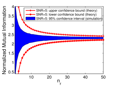
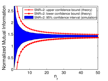
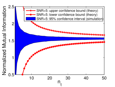
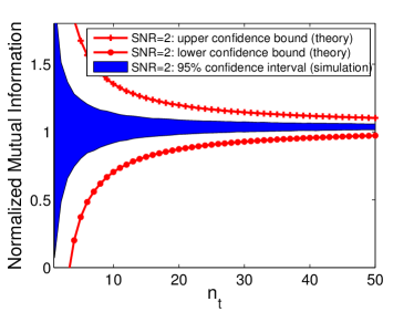
(a) (b) (c) (d)

Figure 1: $95\%$-confidence interval for MIMO mutual information $\frac{C\left(\boldsymbol{H},\small\mathsf{SNR}\right)}{n_{r}}$ when $\boldsymbol{H}$ is drawn from i.i.d. standard Gaussian ensemble. From Table III, the sizes of the upper and lower confidence spans are given by $\frac{\beta\sqrt{\small\mathsf{SNR}}}{\sqrt{\alpha}n_{\mathrm{r}}}$ ($\alpha>1$) and $\frac{\beta\sqrt{\small\mathsf{SNR}}}{n_{\mathrm{r}}}$ ($\alpha<1$), respectively, where $\beta=\sqrt{\log\frac{8}{\left(1-5\%\right)}}$. The expected value of $\frac{C\left(\boldsymbol{H},\small\mathsf{SNR}\right)}{n_{r}}$ is adopted from the mean of 3000 Monte Carlo trials. The theoretical confidence bounds are compared against the simulation results (with 3000 Monte Carlo trials). The results are shown for (a) $\alpha=2$, $\mbox{$\mathsf{SNR}$}=5$; (b) $\alpha=2$, $\mbox{$\mathsf{SNR}$}=2$; (c) $\alpha=1/2$, $\mbox{$\mathsf{SNR}$}=5$; and (d) $\alpha=1/2$, $\mbox{$\mathsf{SNR}$}=2$.

At moderate-to-high SNR, the function $\mathcal{R}(\epsilon,n,m)$ admits a simple approximation. This observation leads to a concise and informative characterization of the mutual information of the MIMO channel, as stated in the following corollary.

Corollary 1.

Suppose that $\mbox{$\mathsf{SNR}$}>\frac{2}{e}\max\left\{\alpha,1\right\}\cdot\max\left\{e^{2}\alpha^{3},4\alpha\right\}$, and set $n:=\min\{n_{\mathrm{t}},n_{\mathrm{r}}\}$.

(a) Consider the assumptions of Theorem 2(a). For any $\beta>8\sqrt{\pi}$,

$$\small\frac{C\left(\boldsymbol{H},\mbox{$\mathsf{SNR}$}\right)}{n_{\mathrm{r}}}\in\begin{cases}\log\frac{\mbox{\small$\mathsf{SNR}$}}{e}+\left(\alpha-1\right)\log\left(\frac{\alpha}{\alpha-1}\right)+\\ \quad\left[\gamma_{\mathrm{bd}}^{\mathrm{lb},+}+\frac{\beta r_{\mathrm{bd}}^{\mathrm{lb},+}}{n_{\mathrm{r}}},\gamma_{\mathrm{bd}}^{\mathrm{ub},+}+\frac{\beta r_{\mathrm{bd}}^{\mathrm{ub},+}}{n_{\mathrm{r}}}\right],&\text{if }\alpha\geq 1,\\ \\ \alpha\log\frac{\small\mathsf{SNR}}{\alpha e}+\left(1-\alpha\right)\log\left(\frac{1}{1-\alpha}\right)+\\ \quad\left[\gamma_{\mathrm{bd}}^{\mathrm{lb},-}+\frac{\beta r_{\mathrm{bd}}^{\mathrm{lb},-}}{n_{\mathrm{r}}},\gamma_{\mathrm{bd}}^{\mathrm{ub},-}+\frac{\beta r_{\mathrm{bd}}^{\mathrm{ub},-}}{n_{\mathrm{r}}}\right],&\text{if }\alpha<1,\end{cases}$$ (44)

with probability exceeding $1-8\exp\left(-\frac{\beta^{2}}{8}\right)$.

(b) Consider the assumptions of Theorem 2(b). For any $\beta>0$,

$$\small\frac{C\left(\boldsymbol{H},\mbox{$\mathsf{SNR}$}\right)}{n_{\mathrm{r}}}\in\begin{cases}\log\frac{\small\mathsf{SNR}}{e}+\left(\alpha-1\right)\log\left(\frac{\alpha}{\alpha-1}\right)+\\ \quad\left[\gamma_{\mathrm{ls}}^{\mathrm{lb},+}+\frac{\beta r_{\mathrm{ls}}^{\mathrm{lb},+}}{n_{\mathrm{r}}},\gamma_{\mathrm{ls}}^{\mathrm{ub},+}+\frac{\beta r_{\mathrm{ls}}^{\mathrm{ub},+}}{n_{\mathrm{r}}}\right],\quad&\text{if }\alpha\geq 1,\\ \\ \alpha\log\frac{\small\mathsf{SNR}}{\alpha e}+\left(1-\alpha\right)\log\left(\frac{1}{1-\alpha}\right)+\\ \quad\left[\gamma_{\mathrm{ls}}^{\mathrm{lb},-}+\frac{\beta r_{\mathrm{ls}}^{\mathrm{lb},-}}{n_{\mathrm{r}}},\gamma_{\mathrm{ls}}^{\mathrm{ub},-}+\frac{\beta r_{\mathrm{ls}}^{\mathrm{ub},-}}{n_{\mathrm{r}}}\right],&\text{if }\alpha<1,\end{cases}$$ (45)

with probability exceeding $1-4\exp\left(-\beta^{2}\right)$.

(c) Consider the assumptions of Theorem 2(c). Then, one has

$$\small\frac{C\left(\boldsymbol{H},\mbox{$\mathsf{SNR}$}\right)}{n_{\mathrm{r}}}\in\begin{cases}\log\frac{\small\mathsf{SNR}}{e}+\left(\alpha-1\right)\log\left(\frac{\alpha}{\alpha-1}\right)+\log\sigma_{\mathrm{c}}+\\ \quad\left[\gamma_{\mathrm{ht}}^{\mathrm{lb},+}+\frac{r_{\mathrm{ht}}^{\mathrm{lb},+}}{n_{\mathrm{r}}},\gamma_{\mathrm{ht}}^{\mathrm{ub},+}+\frac{r_{\mathrm{ht}}^{\mathrm{ub},+}}{n_{\mathrm{r}}}\right],\quad\quad\text{if }\alpha\geq 1,\\ \\ \alpha\log\frac{\small\mathsf{SNR}}{\alpha e}+\left(1-\alpha\right)\log\left(\frac{1}{1-\alpha}\right)+\log\sigma_{\mathrm{c}}+\\ \quad\left[\gamma_{\mathrm{ht}}^{\mathrm{lb},-}+\frac{r_{\mathrm{ht}}^{\mathrm{lb},-}}{n_{\mathrm{r}}},\gamma_{\mathrm{ht}}^{\mathrm{ub},-}+\frac{r_{\mathrm{ht}}^{\mathrm{ub},-}}{n_{\mathrm{r}}}\right],\quad\quad\text{if }\alpha<1,\end{cases}$$ (46)

with probability at least $1-10n^{-c(n)}$.

Here, the residual terms are formally provided in Table III.

Proof.

See Appendix F. ∎

Remark 7.

One can see that the magnitudes of all these extra residual terms $\gamma_{\mathrm{bd}}^{\mathrm{ub},-}$, $\gamma_{\mathrm{bd}}^{\mathrm{lb},-}$, $\gamma_{\mathrm{bd}}^{\mathrm{ub},+}$, $\gamma_{\mathrm{bd}}^{\mathrm{lb},+}$, $\gamma_{\mathrm{ls}}^{\mathrm{ub},-}$, $\gamma_{\mathrm{ls}}^{\mathrm{lb},-}$, $\gamma_{\mathrm{ls}}^{\mathrm{ub},+}$, and $\gamma_{\mathrm{ls}}^{\mathrm{lb},+}$ are no worse than the order

$$\mathcal{O}\left(\frac{\log n}{n}+\small\frac{\log\small\mathsf{SNR}}{\sqrt{\small\mathsf{SNR}}}\right),$$ (47)

which vanish as SNR and channel dimensions grow.

In fact, Corollary 1 is established based on the simple approximation of $\mathcal{R}\left(\epsilon,n,m\right):=\mathbb{E}\left[\det\left(\epsilon\boldsymbol{I}+\frac{1}{m}\boldsymbol{M}\boldsymbol{M}^{*}\right)\right]$. At moderate-to-high SNR, this function can be approximated reasonably well through much simpler expressions, as stated in the following lemma.

Lemma 3.

Consider a random matrix $\boldsymbol{M}=\left(\boldsymbol{M}_{ij}\right)_{1\leq i\leq n,1\leq j\leq m}$ such that $\alpha:=m/n\geq 1$. Suppose that $\boldsymbol{M}_{ij}$’s are independent satisfying $\mathbb{E}\left[\boldsymbol{M}_{ij}\right]=0$ and $\mathbb{E}\left[\left|\boldsymbol{M}_{ij}\right|^{2}\right]=1$. If $\frac{4}{n}<\epsilon<\min\left\{\frac{1}{e^{2}\alpha^{3}},\frac{1}{4\alpha}\right\}$, then one has

$$\frac{1}{n}\log\mathbb{E}\left[\det\left(\epsilon\boldsymbol{I}+\frac{1}{m}\boldsymbol{M}\boldsymbol{M}^{*}\right)\right]$$

$$\quad=\left(\alpha-1\right)\log\left(\frac{\alpha}{\alpha-1}\right)-1+r_{\mathrm{E}},$$ (48)

where the residual term $r_{\mathrm{E}}$ satisfies

$$r_{\mathrm{E}}\in\small\left[\frac{\frac{1}{2}\log n-\log\frac{1}{2\pi}\left(m+1\right)}{n},\frac{1.5\log\left(en\right)}{n}+2\sqrt{\alpha\epsilon}\log\frac{1}{\alpha\epsilon}\right].$$

Proof.

Appendix F.∎

Combining Theorem 2 and Lemma 3 immediately establishes Corollary 1.

IV-A1 Implications of Theorem 2 and Corollary 1

Some implications of Corollary 1 are listed as follows.

1. When we set $\beta=\Theta\left(\sqrt{\frac{\log n}{n}}\right)$, Corollary 1 implies that in the presence of moderate-to-high SNR and moderate-to-large channel dimensionality $n=\min\left\{n_{\mathrm{t}},n_{\mathrm{r}}\right\}$, the information rate per receive antenna behaves like

   $$\footnotesize\frac{C\left(\boldsymbol{H},\mbox{$\mathsf{SNR}$}\right)}{n_{\mathrm{r}}} =\begin{cases}\log\frac{\small\mathsf{SNR}}{e}+\left(\alpha-1\right)\log\left(\frac{\alpha}{\alpha-1}\right)+\\ \text{ }\mathcal{O}\left(\frac{\small\mathsf{SNR}+\sqrt{\log n}}{n}+\frac{\log\small\mathsf{SNR}}{\sqrt{\small\mathsf{SNR}}}\right),\text{ }\text{if }\alpha\geq 1\\ \\ \alpha\log\frac{\small\mathsf{SNR}}{\alpha e}+\left(1-\alpha\right)\log\left(\frac{1}{1-\alpha}\right)+\\ \text{ }\mathcal{O}\left(\frac{\small\mathsf{SNR}+\sqrt{\log n}}{n}+\frac{\log\small\mathsf{SNR}}{\sqrt{\small\mathsf{SNR}}}\right),\text{ }\text{if }\alpha<1\end{cases}$$ (49)

   with high probability. That said, for a fairly large regime, the mutual information falls within a narrow range. In fact, the mutual information depends almost only on $\mathsf{SNR}$ and the ratio $\alpha=\frac{n_{\mathrm{t}}}{n_{\mathrm{r}}}$, and is independent of the precise number of antennas $n_{\mathrm{r}}$ and $n_{\mathrm{t}}$, except for some vanishingly small residual terms. The first-order term of the expression (49) coincides with existing asymptotic results (e.g. [11]). This in turns validates our concentration of measure approach.

2. Theorem 2 indicates that the size of the typical confidence interval for $\frac{C\left(\boldsymbol{H},\small\mathsf{SNR}\right)}{n_{\mathrm{r}}}$ decays with $n$ at a rate not exceeding $\mathcal{O}\left(\frac{1}{n}\right)$ (by picking $\beta=\Theta\left(1\right)$) under measures of bounded support or measures satisfying the LSI. Note that it has been established (e.g. [35, Theorem 2 and Proposition 2]) that the asymptotic standard deviation of $\frac{C\left(\boldsymbol{H},\small\mathsf{SNR}\right)}{n_{\mathrm{r}}}$ scales as $\Theta\left(\frac{1}{n}\right)$. This reveals that the concentration of measure approach we adopt is able to obtain the confidence interval with optimal size. Recent works by Li, Mckay and Chen [74, 75] derive polynomial expansion for each of the moments (e.g. mean, standard deviation, and skewness) of MIMO mutual information, which can also be used to approximate the distributions. In contrast, our results are able to characterize any concentration interval in a simpler and more informative manner.

3. Define the power offset for any channel dimension as follows

   $$\mathcal{L}\left(\boldsymbol{H},\mbox{$\mathsf{SNR}$}\right):=\log\mbox{$\mathsf{SNR}$}-\frac{C\left(\boldsymbol{H},\small\mathsf{SNR}\right)}{\min\left\{n_{\mathrm{r}},n_{\mathrm{t}}\right\}}.$$ (50)

   One can see that this converges to the notion of high-SNR power offset investigated by Lozano et. al. [5, 12]) in the limiting regime (i.e. when $\mathrm{SNR}\rightarrow\infty$). Our results reveal the fluctuation of $\mathcal{L}\left(\boldsymbol{H},\mbox{$\mathsf{SNR}$}\right)$ such that

   $$\small\mathcal{L}\left(\boldsymbol{H},\mbox{$\mathsf{SNR}$}\right)=\begin{cases}\left(\alpha-1\right)\log\left(\frac{\alpha-1}{\alpha}\right)+1+\\ \text{ }\text{ }\mathcal{O}\left(\frac{\small\mathsf{SNR}+\sqrt{\log n}}{n}+\frac{\log\small\mathsf{SNR}}{\sqrt{\small\mathsf{SNR}}}\right),\text{ if }\alpha\geq 1\\ \\ \frac{1-\alpha}{\alpha}\log\left(1-\alpha\right)+\log\left(e\alpha\right)+\\ \text{ }\text{ }\mathcal{O}\left(\frac{\small\mathsf{SNR}+\sqrt{\log n}}{n}+\frac{\log\small\mathsf{SNR}}{\sqrt{\small\mathsf{SNR}}}\right),\text{ if }\alpha<1\end{cases}$$ (51)

   with high probability. The first-order term of $\mathcal{L}\left(\boldsymbol{H},\mbox{$\mathsf{SNR}$}\right)$ agrees with the known results on asymptotic power offset (e.g. [5, Proposition 2][12, Equation (84)]) when $n\rightarrow\infty$ and $\mbox{$\mathsf{SNR}$}\rightarrow\infty$. Our results distinguish from existing results in the sense that we can accurately accommodate a much larger regime beyond the one with asymptotically large SNR and channel dimensions.

4. The same mutual information and power offset values are shared among a fairly general class of distributions even in the non-asymptotic regime. Moreover, heavy-tailed distributions lead to well-controlled information rate and power-offset as well, although the spectral measure concentration is often less sharp than for sub-Gaussian distributions (which ensure exponentially sharp concentration).

5. Finally, we note that Corollary 1 not only characterizes the order of the residual term, but also provides reasonably accurate characterization of a narrow confidence interval such that the mutual information and the power offset lies within it, with high probability. All pre-constants are explicitly provided, resulting in a full assessment of the mutual information and the power offset. Our results do not rely on careful choice of growing matrix sequences, which are typically required in those works based on asymptotic laws.

IV-A2 Connection to the General Framework

We now illustrate how the proof of Theorem 2 follows from the general framework presented in Section III.

1. Note that the mutual information can be alternatively expressed as

   $$\frac{1}{n_{\mathrm{r}}}C\left(\boldsymbol{H},\mbox{$\mathsf{SNR}$}\right)$$

   $$\quad=\frac{1}{n_{\mathrm{r}}}\sum_{i=1}^{\min\left\{n_{\mathrm{r}},n_{\mathrm{t}}\right\}}\log\left(1+\mbox{$\mathsf{SNR}$}\cdot\lambda_{i}\left(\frac{1}{n_{\mathrm{t}}}\boldsymbol{H}\boldsymbol{H}^{*}\right)\right)$$

   $$\quad:=\frac{1}{n_{\mathrm{r}}}\sum_{i=1}^{\min\left\{n_{\mathrm{r}},n_{\mathrm{t}}\right\}}\left\{\log\mbox{$\mathsf{SNR}$}+f\left(\lambda_{i}\left(\frac{1}{n_{\mathrm{t}}}\boldsymbol{H}\boldsymbol{H}^{*}\right)\right)\right\},$$

   where $f\left(x\right):=\log\left(\frac{1}{\small\mathsf{SNR}}+x\right)$ on the domain $x\geq 0$. As a result, the function $g(x):=f(x^{2})=\log\left(\frac{1}{\small\mathsf{SNR}}+x^{2}\right)$ has Lipschitz norm $\left\|g\right\|_{\mathcal{L}}\leq\small\mathsf{SNR}^{1/2}$.

2. For measures satisfying the LSI, Theorem 2(b) immediately follows from Theorem 1(b). For measures of bounded support or heavy-tailed measures, one can introduce the following auxiliary function with respect to some small $\epsilon$:

   $$g_{\epsilon}(x):=\begin{cases}\log\left(\epsilon+x^{2}\right),&\text{if }x\geq\sqrt{\epsilon},\\ \frac{1}{\sqrt{\epsilon}}\left(x-\sqrt{\epsilon}\right)+\log\left(2\epsilon\right),\quad&\text{if }0\leq x<\sqrt{\epsilon},\end{cases}$$

   which is obtained by convexifying $g(x)$. If we set $f_{\epsilon}(x):=g_{\epsilon}(\sqrt{x})$, then one can easily check that

   $$f_{\small\mathsf{SNR}^{-1}}\left(x\right)\leq f\left(x\right)\leq f_{\frac{e}{2}\small\mathsf{SNR}^{-1}}\left(x\right).$$

   Applying Theorem 1(a) allows us to derive the concentration on

   $$\frac{1}{n_{\mathrm{r}}}\sum_{i=1}^{\min\left\{n_{\mathrm{r}},n_{\mathrm{t}}\right\}}f_{\small\mathsf{SNR}^{-1}}\left(\lambda_{i}\left(\frac{1}{n_{\mathrm{t}}}\boldsymbol{H}\boldsymbol{H}^{*}\right)\right)$$

   and

   $$\frac{1}{n_{\mathrm{r}}}\sum_{i=1}^{\min\left\{n_{\mathrm{r}},n_{\mathrm{t}}\right\}}f_{\frac{e}{2}\small\mathsf{SNR}^{-1}}\left(\lambda_{i}\left(\frac{1}{n_{\mathrm{t}}}\boldsymbol{H}\boldsymbol{H}^{*}\right)\right),$$

   which in turn provide tight lower and upper bounds for $\frac{1}{n_{\mathrm{r}}}\sum_{i=1}^{\min\left\{n_{\mathrm{r}},n_{\mathrm{t}}\right\}}f\left(\lambda_{i}\left(\frac{1}{n_{\mathrm{t}}}\boldsymbol{H}\boldsymbol{H}^{*}\right)\right)$.

3. Finally, the mean value $\mathbb{E}\left[\mathrm{det}\left(\boldsymbol{I}+\mbox{$\mathsf{SNR}$}\cdot\frac{1}{n_{\mathrm{t}}}\boldsymbol{H}\boldsymbol{H}^{*}\right)\right]$ admits a closed-form expression independent of precise entry distributions, as derived in Lemma 2.

IV-B MMSE Estimation in Random Vector Channels

Next, we show that our analysis framework can be applied in Bayesian inference problems that involve estimation of uncorrelated signals components. Consider a simple linear vector channel model

$$\boldsymbol{y}=\boldsymbol{H}\boldsymbol{x}+\boldsymbol{z},$$

where $\boldsymbol{H}\in\mathbb{C}^{n\times p}$ is a known matrix, $\boldsymbol{x}\in\mathbb{C}^{p}$ denotes an input signal with zero mean and covariance matrix $P\boldsymbol{I}_{p}$, and $\boldsymbol{z}$ represents a zero-mean noise uncorrelated with $\boldsymbol{x}$, which has covariance $\sigma^{2}\boldsymbol{I}_{n}$. Here, we denote by $p$ and $n$ the input dimension and the sample size, respectively, which agrees with the conventional notation adopted in the statistics community. In this subsection, we assume that

$$\alpha:=\frac{p}{n}\leq 1,$$ (52)

i.e. the sample size exceeds the dimension of the input signal. The goal is to estimate the channel input $\boldsymbol{x}$ from the channel output $\boldsymbol{y}$ with minimum $\ell_{2}$ distortion.

The MMSE estimate of $\boldsymbol{x}$ given $\boldsymbol{y}$ can be written as [4]

$$\hat{\boldsymbol{x}} =\mathbb{E}\left[\boldsymbol{x}\mid\boldsymbol{y}\right]=\mathbb{E}\left[\boldsymbol{x}\boldsymbol{y}^{*}\right]\left(\mathbb{E}\left[\boldsymbol{y}\boldsymbol{y}^{*}\right]\right)^{-1}\boldsymbol{y}$$

$$=P\boldsymbol{H}^{*}\left(\sigma^{2}\boldsymbol{I}_{n}+P\boldsymbol{H}\boldsymbol{H}^{*}\right)^{-1}\boldsymbol{y},$$ (53)

and the resulting MMSE is given by

$$\small\mbox{$\mathsf{MMSE}$}\left(\boldsymbol{H},\mbox{$\mathsf{SNR}$}\right) =\small\mathrm{tr}\left(P\boldsymbol{I}_{p}-P^{2}\boldsymbol{H}^{*}\left(\sigma^{2}\boldsymbol{I}_{n}+P\boldsymbol{H}\boldsymbol{H}^{*}\right)^{-1}\boldsymbol{H}\right).$$ (54)

The normalized MMSE (NMMSE) can then be written as

$$\mbox{$\mathsf{NMMSE}$}\left(\boldsymbol{H},\mbox{$\mathsf{SNR}$}\right):=\frac{\mbox{$\mathsf{MMSE}$}\left(\boldsymbol{H},\small\mathsf{SNR}\right)}{\mathbb{E}\left[\left\|\boldsymbol{x}\right\|^{2}\right]}$$

$$\quad=\mathrm{tr}\left(\boldsymbol{I}_{p}-\boldsymbol{H}^{*}\left(\frac{1}{\small\mathsf{SNR}}\boldsymbol{I}_{n}+\boldsymbol{H}\boldsymbol{H}^{*}\right)^{-1}\boldsymbol{H}\right),$$ (55)

where

$$\mbox{$\mathsf{SNR}$}:=\frac{P}{\sigma^{2}}.$$

Using the concentration of measure technique, we can evaluate $\mbox{$\mathsf{NMMSE}$}\left(\boldsymbol{H}\right)$ to within a narrow interval with high probability, as stated in the following theorem.

Theorem 3.

Suppose that $\boldsymbol{H}=\boldsymbol{A}\boldsymbol{M}$, where $\boldsymbol{A}\in\mathbb{C}^{m\times n}$ is a deterministic matrix for some integer $m\geq p$, and $\boldsymbol{M}\in\mathbb{C}^{n\times p}$ is a random matrix such that $\boldsymbol{M}_{ij}$’s are independent random variables satisfying $\mathbb{E}\left[\boldsymbol{M}_{ij}\right]=0$ and $\mathbb{E}[\left|\boldsymbol{M}_{ij}\right|^{2}]=\frac{1}{p}$.

(a) If $\sqrt{p}\boldsymbol{M}_{ij}$’s are bounded by $D$, then for any $\beta>8\sqrt{\pi}$,

$$\small\frac{\mbox{$\mathsf{NMMSE}$}\left(\boldsymbol{H},\small\mathsf{SNR}\right)}{p}\in \small\left[\mathcal{M}\left(\frac{8}{9\small\mathsf{SNR}},\boldsymbol{H}\right)+\frac{\beta\tau_{\mathrm{bd}}^{\mathrm{lb}}}{p},\right.$$

$$\small\left.\quad\mathcal{M}\left(\frac{9}{8\small\mathsf{SNR}},\boldsymbol{H}\right)+\frac{\beta\tau_{\mathrm{bd}}^{\mathrm{ub}}}{p}\right]$$ (56)

with probability exceeding $1-8\exp\left(-\frac{\beta^{2}}{16}\right)$.

(b) If $\sqrt{p}\boldsymbol{M}_{ij}$’s satisfy the LSI with respect to a uniform constant $c_{\mathrm{ls}}$, then for any $\beta>0$,

$$\small\frac{\mbox{$\mathsf{NMMSE}$}\left(\boldsymbol{H},\small\mathsf{SNR}\right)}{p}\in\mathcal{M}\left(\frac{1}{\small\mathsf{SNR}},\boldsymbol{H}\right)+\frac{\beta}{p}\left[\tau_{\mathrm{ls}}^{\mathrm{lb}},\tau_{\mathrm{ls}}^{\mathrm{ub}}\right]$$ (57)

with probability exceeding $1-4\exp\left(-\frac{\beta^{2}}{2}\right)$.

(c) Suppose that $\sqrt{p}\boldsymbol{M}_{ij}$’s are independently drawn from either sub-exponential distributions or heavy-tailed distributions and that the distributions are symmetric about 0. Let $\tau_{c}$ be defined as in (7) with respect to $\sqrt{p}\boldsymbol{M}_{ij}$’s for some sequence $c(n)$. Then

$$\small\frac{\mbox{$\mathsf{NMMSE}$}\left(\boldsymbol{H},\small\mathsf{SNR}\right)}{p}\in\small \left[\small\mathcal{M}\left(\frac{8}{9\small\mathsf{SNR}},\boldsymbol{A}\tilde{\boldsymbol{M}}\right)+\frac{\tau_{\mathrm{ht}}^{\mathrm{lb}}}{p},\right.$$

$$\small\left.\quad\small\mathcal{M}\left(\frac{9}{8\small\mathsf{SNR}},\boldsymbol{A}\tilde{\boldsymbol{M}}\right)+\frac{\tau_{\mathrm{ht}}^{\mathrm{ub}}}{p}\right]$$ (58)

with probability exceeding $1-\frac{10}{p^{c(n)}}$, where $\tilde{\boldsymbol{M}}$ is defined such that $\tilde{\boldsymbol{M}}_{ij}:=\boldsymbol{M}_{ij}{\bf 1}{}_{\left\{\sqrt{p}\left|\boldsymbol{M}_{ij}\right|<\tau_{c}\right\}}$.

Here, the function $\mathcal{M}\left(\epsilon,\boldsymbol{H}\right)$ is defined as

$$\mathcal{M}\left(\delta,\boldsymbol{H}\right):=\frac{1}{p}\mathbb{E}\left[\mathrm{tr}\left(\left(\delta\boldsymbol{I}+\boldsymbol{H}^{*}\boldsymbol{H}\right)^{-1}\right)\right],$$ (59)

and the residual terms are formally defined in Table IV.

Proof.

See Appendix G.∎

Theorem 3 ensures that the MMSE per signal component falls within a small interval with high probability. This concentration phenomenon again arises for a very large class of probability measures including bounded distributions, sub-Gaussian distributions, and heavy-tailed distributions. Note that $\mathcal{M}\left(\frac{9}{8\small\mathsf{SNR}},\boldsymbol{H}\right)$, $\mathcal{M}\left(\frac{8}{9\small\mathsf{SNR}},\boldsymbol{H}\right)$, and $\mathcal{M}\left(\frac{1}{\small\mathsf{SNR}},\boldsymbol{H}\right)$ are often very close to each other at moderate-to-high SNR (e.g. see the analysis of Corollary 2). The spans of the residual intervals for both bounded and logarithmic Sobolev measures do not exceed the order

$$\mathcal{O}\left(\frac{\beta\left\|\boldsymbol{A}\right\|\mbox{$\mathsf{SNR}$}^{1.5}}{p}\right),$$ (60)

which is often negligible compared with the MMSE value per signal component.

In general, we are not aware of a closed-form expression for $\mathcal{M}\left(\delta,\boldsymbol{H}\right)$ under various random matrix ensembles. If $\boldsymbol{H}$ is drawn from a Gaussian ensemble, however, we are able to derive a simple expression and bound this value to within a narrow confidence interval with high probability, as follows.

Corollary 2.

Suppose that $\boldsymbol{H}_{ij}\sim\mathcal{N}\left(0,\frac{1}{p}\right)$ are independent Gaussian random variables, and assume that $\alpha<1$. Then

$$\frac{\mbox{$\mathsf{NMMSE}$}\left(\boldsymbol{H},\mbox{$\mathsf{SNR}$}\right)}{p}\in\frac{\alpha}{1-\alpha}+\left[\tau_{\mathrm{g}}^{\mathrm{lb}}+\frac{\beta\tau_{\mathrm{ls}}^{\mathrm{lb}}}{p},\tau_{\mathrm{g}}^{\mathrm{ub}}+\frac{\beta\tau_{\mathrm{ls}}^{\mathrm{ub}}}{p}\right]$$ (61)

with probability exceeding $1-4\exp\left(-\frac{\beta^{2}}{2}\right)$. Here, $\tau_{\mathrm{g}}^{\mathrm{lb}}$ and $\tau_{\mathrm{g}}^{\mathrm{ub}}$ are presented in Theorem 3, while $\tau_{\mathrm{g}}^{\mathrm{lb}}$ and $\tau_{\mathrm{g}}^{\mathrm{ub}}$ are formally defined in Table IV.

Proof.

See Appendix G.∎

Table IV: Summary of parameters of Theorem 3 and Corollary 2.

Theorem 3	$\tau_{\mathrm{bd}}^{\mathrm{lb}}:=-\frac{2\sqrt{2}D\left\|\boldsymbol{A}\right\|\small\mathsf{SNR}^{1.5}}{3\sqrt{3}}$	$\tau_{\mathrm{bd}}^{\mathrm{ub}}:=\frac{3\sqrt{3}D\left\|\boldsymbol{A}\right\|\small\mathsf{SNR}^{1.5}}{8}$
	$\tau_{\mathrm{ls}}^{\mathrm{lb}}:=-\frac{3\sqrt{3}\sqrt{c_{\mathrm{ls}}}\left\|\boldsymbol{A}\right\|\small\mathsf{SNR}^{1.5}}{8}$	$\tau_{\mathrm{ls}}^{\mathrm{ub}}:=-\frac{3\sqrt{3}\sqrt{c_{\mathrm{ls}}}\left\|\boldsymbol{A}\right\|\small\mathsf{SNR}^{1.5}}{8}$
	$\tau_{\mathrm{ht}}^{\mathrm{lb}}:=-\frac{8\sqrt{2}\tau_{c}\sigma_{c}\left\|\boldsymbol{A}\right\|\sqrt{c(n)\log n}\small\mathsf{SNR}^{1.5}}{3\sqrt{3}}$	$\tau_{\mathrm{ht}}^{\mathrm{ub}}:=\frac{3\sqrt{3}\tau_{c}\sigma_{c}\left\|\boldsymbol{A}\right\|\sqrt{c(n)\log n}\small\mathsf{SNR}^{1.5}}{2}$
Corollary 2	$\tau_{\mathrm{g}}^{\mathrm{ub}}:=\frac{\alpha}{n\left(1-\alpha-\frac{1}{n}\right)^{2}}$	$\tau_{\mathrm{g}}^{\mathrm{lb}}:=-\frac{\alpha^{2}}{\small\mathsf{SNR}\left(1-\alpha-\frac{3}{n}\right)^{3}}$

Corollary 2 implies that the MMSE per signal component behaves like

$$\small\frac{\mbox{$\mathsf{NMMSE}$}\left(\boldsymbol{H},\small\mathsf{SNR}\right)}{p}=\frac{\alpha}{1-\alpha}+\small\mathcal{O}\left(\frac{\small\mathsf{SNR}^{1.5}}{n}+\frac{1}{n}+\frac{1}{\small\mathsf{SNR}}\right)$$

with high probability (by setting $\beta=\Theta\left(1\right)$). Except for the residual term that vanishes in the presence of high SNR and large signal dimensionality $n$, the first order term depends only on the SNR and the oversampling ratio $\frac{1}{\alpha}$. Therefore, the normalized MMSE converges to an almost deterministic value even in the non-asymptotic regime. This illustrates the effectiveness of the proposed analysis approach.

IV-B1 Connection to the General Framework

We now demonstrate how the proof of Theorem 3 follows from the general template presented in Section III.

1. Observe that the MMSE can be alternatively expressed as

   $$\small\frac{\mbox{$\mathsf{NMMSE}$}\left(\boldsymbol{H},\small\mathsf{SNR}\right)}{p} =\frac{1}{p}\sum_{i=1}^{\min\left\{n,p\right\}}\frac{1}{\small\mathsf{SNR}^{-1}+\lambda_{i}\left(\boldsymbol{H}\boldsymbol{H}^{*}\right)}$$

   $$:=\frac{1}{p}\sum_{i=1}^{\min\left\{n,p\right\}}f\left(\lambda_{i}\left(\boldsymbol{H}\boldsymbol{H}^{*}\right)\right),$$

   where $f\left(x\right):=\frac{1}{\small\mathsf{SNR}^{-1}+x}$ $(x\geq 0)$. Consequently, the function $g(x):=f(x^{2})=\frac{1}{\small\mathsf{SNR}^{-1}+x^{2}}$ has Lipschitz norm $\left\|g\right\|_{\mathcal{L}}\leq\frac{3\sqrt{3}}{8}\small\mbox{$\mathsf{SNR}$}^{3/2}$.

2. For measures satisfying the LSI, Theorem 3(b) can be immediately obtained by Proposition 1(b). For measures of bounded support or heavy-tailed measures, one can introduce the following auxiliary function with respect to some small $\epsilon$:

   $$\tilde{g}_{\epsilon}(x):=\begin{cases}\frac{1}{\epsilon^{2}+x^{2}},&\text{if }x>\frac{1}{\sqrt{3}}\epsilon,\\ -\frac{3\sqrt{3}}{8}\left(x-\frac{\epsilon}{\sqrt{3}}\right)+\frac{3}{4\epsilon^{2}},\quad&\text{if }x\leq\frac{1}{\sqrt{3}}\epsilon,\end{cases}$$

   which is obtained by convexifying $g(x)$. By setting $\tilde{f}_{\epsilon}(x):=\tilde{g}_{\epsilon}(\sqrt{x})$, one has

   $$\tilde{f}_{\frac{3}{2\sqrt{2}}\small\mathsf{SNR}^{-1/2}}\left(x\right)\leq f\left(x\right)\leq\tilde{f}_{\small\mathsf{SNR}^{-1/2}}\left(x\right).$$

   Applying Proposition 1(a) gives the concentration bounds on

   $$\frac{1}{p}\sum_{i=1}^{\min\left\{p,n\right\}}\tilde{f}_{\frac{3}{2\sqrt{2}}\small\mathsf{SNR}^{-1/2}}\left(\lambda_{i}\left(\boldsymbol{H}\boldsymbol{H}^{*}\right)\right)$$

   and

   $$\frac{1}{p}\sum_{i=1}^{\min\left\{p,n\right\}}\tilde{f}_{\small\mathsf{SNR}^{-1/2}}\left(\lambda_{i}\left(\boldsymbol{H}\boldsymbol{H}^{*}\right)\right),$$

   which in turn provide tight sandwich bounds for $\frac{1}{p}\sum_{i=1}^{\min\left\{p,n\right\}}f\left(\lambda_{i}\left(\boldsymbol{H}\boldsymbol{H}^{*}\right)\right)$.

V Conclusions and Future Directions

We have presented a general analysis framework that allows many canonical MIMO system performance metrics taking the form of linear spectral statistics to be assessed within a narrow concentration interval. Moreover, we can guarantee that the metric value falls within the derived interval with high probability, even under moderate channel dimensionality. We demonstrate the effectiveness of the proposed framework through two canonical metrics in wireless communications and signal processing: mutual information and power offset of MIMO channels, and MMSE for Gaussian processes. For each of these examples, our approach allows a more refined and accurate characterization than those derived in previous work in the asymptotic dimensionality limit. While our examples here are presented for i.i.d. channel matrices, they can all be immediately extended to accommodate dependent random matrices using the same techniques. In other words, our analysis can be applied to characterize various performance metrics of wireless systems under correlated fading, as studied in [8].

Our work suggests a few future research directions for different matrix ensembles. Specifically, if the channel matrix $\boldsymbol{H}$ cannot be expressed as a linear correlation model $\boldsymbol{M}\boldsymbol{A}$ for some known matrix $\boldsymbol{A}$ and a random i.i.d. matrix $\boldsymbol{M}$, then it will be of great interest to see whether there is a systematic approach to analyze the concentration of spectral measure phenomenon. For instance, if $\boldsymbol{H}$ consists of independent sub-Gaussian columns but the elements within each column are correlated (i.e. cannot be expressed as a weighted sum of i.i.d. random variables), then it remains to be seen whether generalized concentration of measure techniques (e.g. [52]) can be applied to find confidence intervals for the system performance metrics. The spiked random matrix model [76], which also admits simple asymptotic characterization, is another popular candidate in modeling various system metrics. Another more challenging case is when the rows of $\boldsymbol{H}$ are randomly drawn from a known set of structured candidates. An example is a random DFT ensemble where each row is independently drawn from a DFT matrix, which is frequently encountered in the compressed sensing literature (e.g. [77]). Understanding the spectral concentration of such random matrices could be of great interest in investigating OFDM systems under random subsampling.

Appendix A Proof of Proposition 1

Part (a) and (b) of Proposition 1 are immediate consequences of [51, Corollary 1.8] via simple algebraic manipulation. Here, we only provide the proof for heavy-tailed distributions.

Define a new matrix $\tilde{\boldsymbol{M}}$ as a truncated version of $\boldsymbol{M}$ such that

$$\tilde{\boldsymbol{M}}_{ij}=\begin{cases}\boldsymbol{M}_{ij},\quad&\text{if }\left|\boldsymbol{M}_{ij}\right|<\tau_{c},\\ 0,&\text{otherwise}.\end{cases}$$

Note that the entries of $\tilde{\boldsymbol{M}}$ have zero mean and variance not exceeding $\sigma_{c}^{2}$, and are uniformly bounded in magnitude by $\tau_{c}$. Consequently, Theorem 1(a) asserts that for any $\beta>8\sqrt{\pi}$, we have

$$\left|f_{0}\left(\tilde{\boldsymbol{M}}\right)-\mathbb{E}\left[f_{0}\left(\tilde{\boldsymbol{M}}\right)\right]\right|\leq\frac{\beta\tau_{c}\sigma_{c}\rho\left\|g\right\|_{\mathcal{L}}}{n}$$ (62)

with probability exceeding $1-4\exp\left(-\frac{\beta^{2}}{16}\right)$.

In addition, a simple union bound taken collectively with (7) yields

$$\mathbb{P}\left(\boldsymbol{M}\neq\tilde{\boldsymbol{M}}\right) \leq\sum_{1\leq i\leq n,1\leq j\leq m}\mathbb{P}\left(\frac{1}{\nu_{ij}}\left|\boldsymbol{M}_{ij}\right|>\tau_{c}\right)$$

$$\leq mn\mathbb{P}\left(\frac{1}{\nu_{ij}}\left|\boldsymbol{M}_{ij}\right|>\tau_{c}\right)=\frac{1}{n^{c(n)}}.$$ (63)

By setting $\beta=4\sqrt{c(n)\log n}$, one has

$$4\exp\left(-\frac{\beta^{2}}{16}\right)=\frac{4}{n^{c(n)}}.$$

This combined with (62) and the union bound implies that

$$\left|f_{0}\left(\boldsymbol{M}\right)-\mathbb{E}\left[f_{0}\left(\tilde{\boldsymbol{M}}\right)\right]\right|\leq\frac{4\sqrt{c(n)\log n}\tau_{c}\sigma_{c}\rho\left\|g\right\|_{\mathcal{L}}}{n}$$ (64)

holds with probability at least $1-5n^{-\mathrm{c}(n)}$, as claimed.

Appendix B Proof of Lemma 1

For notational simplicity, define

$$Y: =n\left\{f_{0}\left(\boldsymbol{M}\right)-\mathbb{E}\left[f_{0}\left(\boldsymbol{M}\right)\right]\right\}$$

$$=\sum_{i=1}^{\min\{m,n\}}\left\{f\left(\lambda_{i}\left(\frac{1}{n}\boldsymbol{M}\boldsymbol{R}\boldsymbol{R}^{*}\boldsymbol{M}^{*}\right)\right)\right.$$

$$\quad\quad\quad\quad\quad-\left.\mathbb{E}\left[f\left(\lambda_{i}\left(\frac{1}{n}\boldsymbol{M}\boldsymbol{R}\boldsymbol{R}^{*}\boldsymbol{M}^{*}\right)\right)\right]\right\}$$

and

$$Z:=nf_{0}\left(\boldsymbol{M}\right)=\sum_{i=1}^{\min\{m,n\}}f\left(\lambda_{i}\left(\frac{1}{n}\boldsymbol{M}\boldsymbol{R}\boldsymbol{R}^{*}\boldsymbol{M}^{*}\right)\right),$$

and denote by $\mu_{\left|Y\right|}(y)$ the probability measure of $\left|Y\right|$.

(1) Suppose that $\mathbb{P}\left(\left|Y\right|>y\right)\leq c_{1}\exp\left(-c_{2}y\right)$ holds for some universal constants $c_{1}>0$ and $c_{2}>1$. Applying integration by parts yields the following inequality

$$\mathbb{E}\left[e^{Y}\right] \leq\mathbb{E}\left[e^{\left|Y\right|}\right]={\displaystyle\int}_{0}^{\infty}e^{\left|Y\right|}\mathrm{d}\mu_{\left|Y\right|}(y)$$

$$=-\left.e^{y}\mathbb{P}\left(\left|Y\right|>y\right)\right|_{0}^{\infty}+\int_{0}^{\infty}e^{y}\mathbb{P}\left(\left|Y\right|>y\right)\mathrm{d}y$$

$$\leq 1+c_{1}\int_{0}^{\infty}\exp\left(-\left(c_{2}-1\right)y\right)\mathrm{d}y$$

$$=1+\frac{c_{1}}{c_{2}-1}.$$ (65)

This gives rise to the following bound

$$\log\mathbb{E}\left[e^{Z}\right]-\log e^{\mathbb{E}\left[Z\right]}=\log\mathbb{E}\left[e^{Y}\right]\leq\log\left(1+\frac{c_{1}}{c_{2}-1}\right).$$

Therefore, we can conclude

$$\frac{1}{n}\log\mathbb{E}\left[e^{Z}\right]-\frac{\log\left(1+\frac{c_{1}}{c_{2}-1}\right)}{n}\leq\frac{1}{n}\mathbb{E}\left[Z\right]\leq\frac{1}{n}\log\mathbb{E}\left[e^{Z}\right],$$ (66)

where the last inequality follows from Jensen’s inequality

$$\frac{1}{n}\mathbb{E}\left[Z\right]=\frac{1}{n}\log e^{\mathbb{E}\left[Z\right]}\leq\frac{1}{n}\log\mathbb{E}e^{\left[Z\right]}.$$

(2) Similarly, if $\mathbb{P}\left(\left|Y\right|>y\right)\leq c_{1}\exp\left(-c_{2}y^{2}\right)$ holds for some universal constants $c_{1}>0$ and $c_{2}>0$, then one can bound

$$\mathbb{E}\left[e^{Y}\right] \leq-\left.e^{y}\mathbb{P}\left(\left|Y\right|>y\right)\right|_{0}^{\infty}+\int_{0}^{\infty}e^{y}\mathbb{P}\left(\left|Y\right|>y\right)\mathrm{d}y$$

$$\leq 1+c_{1}\int_{0}^{\infty}\exp\left(-c_{2}y^{2}+y\right)\mathrm{d}y$$

$$\leq 1+c_{1}\sqrt{\frac{\pi}{c_{2}}}\exp\left(\frac{1}{4c_{2}}\right)$$

$$\quad\quad\quad\cdot{\displaystyle\int}_{-\infty}^{\infty}\sqrt{\frac{c_{2}}{\pi}}\exp\left(-c_{2}y^{2}+y-\frac{1}{4c_{2}}\right)\mathrm{d}y$$

$$\leq 1+c_{1}\sqrt{\frac{\pi}{c_{2}}}\exp\left(\frac{1}{4c_{2}}\right),$$ (67)

where the last inequality follows since $\sqrt{\frac{c_{2}}{\pi}}\exp\left(-c_{2}y^{2}+y-\frac{1}{4c_{2}}\right)$ is the pdf of $\mathcal{N}\left(\frac{1}{2c_{2}},\frac{2}{c_{2}}\right)$ and hence integrates to 1.

Applying the same argument as for the measure with sub-exponential tails then leads to

$$\frac{1}{n}\log\mathbb{E}\left[e^{Z}\right] \geq\frac{1}{n}\mathbb{E}\left[Z\right]$$

$$\geq\frac{1}{n}\log\mathbb{E}\left[e^{Z}\right]-\frac{\log\left(1+\sqrt{\frac{c_{1}^{2}\pi}{c_{2}}}\exp\left(\frac{1}{4c_{2}}\right)\right)}{n}.$$

Appendix C Proof of Theorem 1

For notational convenience, define

$$Z :=\sum_{i=1}^{\min\{m,n\}}f\left(\lambda_{i}\left(\frac{1}{n}\boldsymbol{M}\boldsymbol{R}\boldsymbol{R}^{*}\boldsymbol{M}^{*}\right)\right),$$

$$Y :=\text{ }Z-\mathbb{E}\left[Z\right].$$

(1) Under the assumptions of Proposition 1(a), the concentration result (15) implies that for any $y>8\sqrt{\pi}\rho D\left\|g\right\|_{\mathcal{L}}$, one has

$$\mathbb{P}\left(\left|Y\right|>y\right)\leq 4\exp\left(-\frac{y^{2}}{8\kappa D^{2}\rho^{2}\nu^{2}\left\|g\right\|_{\mathcal{L}}^{2}}\right).$$

For $y\leq 8\sqrt{\pi}D\rho\nu\left\|g\right\|_{\mathcal{L}}$, we can employ the trivial bound $\mathbb{P}\left(\left|Y\right|>y\right)\leq 1$. These two bounds taken collectively lead to a universal bound such that for any $y\geq 0$, one has

$$\mathbb{P}\left(\left|Y\right|>y\right)\leq\exp\left(\frac{8\pi}{\kappa}\right)\exp\left(-\frac{y^{2}}{8\kappa D^{2}\rho^{2}\nu^{2}\left\|g\right\|_{\mathcal{L}}^{2}}\right).$$

Lemma 1 then suggests

$$\frac{1}{n}\log\mathcal{E}\left(f\right)\geq\frac{1}{n}\mathbb{E}\left[Z\right]$$

$$\text{ }\geq\frac{\log\mathcal{E}\left(f\right)}{n}-\frac{\log\left(1+\sqrt{8\kappa\pi}D\rho\nu\left\|g\right\|_{\mathcal{L}}e^{\frac{8\pi}{\kappa}+2\kappa D^{2}\rho^{2}\nu^{2}\left\|g\right\|_{\mathcal{L}}^{2}}\right)}{n}.$$

This together with (15) establishes (25).

(2) Under the assumptions of Proposition 1(b), the concentration inequality (15) asserts that for any $y>0$, we have

$$\mathbb{P}\left(\left|Y\right|>y\right)\leq 2\exp\left(-\frac{y^{2}}{\kappa c_{\mathrm{ls}}\rho^{2}\nu^{2}\left\|g\right\|_{\mathcal{L}}^{2}}\right).$$

Applying Lemma 1 then yields

$$\frac{1}{n}\log\mathcal{E}\left(f\right)\geq\frac{1}{n}\mathbb{E}\left[Z\right]$$

$$\text{ }\geq\frac{\log\mathcal{E}\left(f\right)}{n}-\frac{\log\left(1+\sqrt{4\kappa\pi c_{\mathrm{ls}}\rho^{2}\nu^{2}\left\|g\right\|_{\mathcal{L}}^{2}}e^{\frac{\kappa}{4}c_{\mathrm{ls}}\rho^{2}\nu^{2}\left\|g\right\|_{\mathcal{L}}^{2}}\right)}{n}.$$

This combined with (16) establishes (26).

(3) Under the assumptions of Proposition 1(c), define

$$\tilde{Z} :=\sum_{i=1}^{n}f\left(\lambda_{i}\left(\frac{1}{n}\tilde{\boldsymbol{M}}\boldsymbol{R}\boldsymbol{R}^{*}\tilde{\boldsymbol{M}}^{*}\right)\right),$$

$$\tilde{Y} :=\tilde{Z}-\mathbb{E}\left[\tilde{Z}\right].$$

Combining the concentration result (62) with (25) gives rise to

$$\begin{cases}\frac{1}{n}\sum_{i=1}^{n}f\left(\lambda_{i}\left(\frac{1}{n}\tilde{\boldsymbol{M}}\boldsymbol{R}\boldsymbol{R}^{*}\tilde{\boldsymbol{M}}^{*}\right)\right)\\ \quad\quad\leq\frac{1}{n}\log\mathcal{E}_{\tilde{\boldsymbol{M}}}\left(f\right)+\frac{\beta\tau_{c}\sigma_{c}\rho\left\|g\right\|_{\mathcal{L}}}{n},\\ \\ \frac{1}{n}\sum_{i=1}^{n}f\left(\lambda_{i}\left(\frac{1}{n}\tilde{\boldsymbol{M}}\boldsymbol{R}\boldsymbol{R}^{*}\tilde{\boldsymbol{M}}^{*}\right)\right)\\ \quad\quad\geq\frac{1}{n}\log\mathcal{E}_{\tilde{\boldsymbol{M}}}\left(f\right)-\frac{\beta\tau_{c}\sigma_{c}\rho\left\|g\right\|_{\mathcal{L}}}{n}-\frac{c_{\rho,f,\tau_{c},\sigma_{c}}}{n},\end{cases}$$ (68)

with probability exceeding $1-4\exp\left(-\frac{\beta^{2}}{8\kappa}\right)$. We have shown in (63) that

$$\mathbb{P}\left(\boldsymbol{M}\neq\tilde{\boldsymbol{M}}\right)\leq\frac{1}{n^{c(n)}}$$

and $4\exp\left(-\frac{\beta^{2}}{8\kappa}\right)=\frac{4}{n^{c(n)}}$ when $\beta=\sqrt{8\kappa c(n)\log n}$, concluding the proof via the union bound.

Appendix D Proof of Lemma 2

For any $n\times n$ matrix $\boldsymbol{A}$ with eigenvalues $\lambda_{1},\cdots,\lambda_{n}$, define the characteristic polynomial of $\boldsymbol{A}$ as

$$p_{\boldsymbol{A}}(t) =\det\left(t\boldsymbol{I}-\boldsymbol{A}\right)=t^{n}-S_{1}(\lambda_{1},\cdots,\lambda_{n})t^{n-1}+\cdots$$

$$\quad\quad\quad\quad\quad\quad\quad\quad+(-1)^{n}S_{n}(\lambda_{1},\cdots,\lambda_{n}),$$ (69)

where $S_{l}(\lambda_{1},\cdots,\lambda_{n})$ is the $l$th elementary symmetric polynomial defined as follows

$$S_{l}(\lambda_{1},\cdots,\lambda_{n}):=\sum_{1\leq i_{1}<\cdots<i_{l}\leq n}\prod_{j=1}^{l}\lambda_{i_{j}}.$$ (70)

Let $E_{l}(\boldsymbol{A})$ represent the sum of determinants of all $l$-by-$l$ principal minors of $\boldsymbol{A}$. It has been shown in [78, Theorem 1.2.12] that

$$S_{l}(\lambda_{1},\cdots,\lambda_{n})=E_{l}(\boldsymbol{A}),\quad\quad 1\leq l\leq n,$$ (71)

which follows that

$$\det\left(t\boldsymbol{I}+\boldsymbol{A}\right)=t^{n}+E_{1}(\boldsymbol{A})t^{n-1}+\cdots+E_{n}(\boldsymbol{A}).$$ (72)

On the other hand, for any principal minor $\left(\boldsymbol{M}\boldsymbol{M}^{*}\right)_{\boldsymbol{s},\boldsymbol{s}}$ of $\boldsymbol{M}\boldsymbol{M}^{*}$ coming from the rows and columns at indices from $\boldsymbol{s}$ (where $\boldsymbol{s}\subseteq[n]$ is an index set), then one can show that

$$\mathbb{E}\left[\det\left(\left(\boldsymbol{M}\boldsymbol{M}^{*}\right)_{\boldsymbol{s},\boldsymbol{s}}\right)\right] =\mathbb{E}\left[\det\left(\boldsymbol{M}_{\boldsymbol{s},[m]}\boldsymbol{M}_{\boldsymbol{s},[m]}^{*}\right)\right]$$

$$=\sum_{\boldsymbol{t}:\mathrm{card}\left(\boldsymbol{t}\right)=\mathrm{card}\left(\boldsymbol{s}\right)}\mathbb{E}\left[\det\left(\boldsymbol{M}_{\boldsymbol{s},\boldsymbol{t}}\boldsymbol{M}_{\boldsymbol{s},\boldsymbol{t}}^{*}\right)\right]$$

$$={m\choose\mathrm{card}(\boldsymbol{s})}\cdot\mathbb{E}\left[\det\left(\boldsymbol{M}_{\boldsymbol{s},\boldsymbol{s}}\boldsymbol{M}_{\boldsymbol{s},\boldsymbol{s}}^{*}\right)\right].$$ (73)

Consider now any i.i.d. random matrix $\boldsymbol{G}\in\mathbb{C}^{l\times l}$ such that $\mathbb{E}\left[\boldsymbol{G}_{ij}\right]=0$ and $\mathbb{E}[\left|\boldsymbol{G}_{ij}\right|^{2}]=1$. If we denote by $\prod_{l}$ the permutation group of $l$ elements, then the Leibniz formula for the determinant gives

$$\det\left(\boldsymbol{G}\right)=\sum_{\sigma\in\prod_{l}}\text{sgn}(\sigma)\prod_{i=1}^{l}\boldsymbol{G}_{i,\sigma(i)}.$$

Since $\boldsymbol{G}_{ij}$ are jointly independent, we have

$$\mathbb{E}\left[\text{det}\left(\boldsymbol{G}\boldsymbol{G}^{*}\right)\right] =\mathbb{E}\left[\left|\det\left(\boldsymbol{G}\right)\right|^{2}\right]$$

$$=\sum_{\sigma\in\prod_{l}}\mathbb{E}\left[\prod_{i=1}^{l}\left|\boldsymbol{G}_{i,\sigma(i)}\right|^{2}\right]$$

$$=\sum_{\sigma\in\prod_{l}}\prod_{i=1}^{l}\mathbb{E}\left[\left|\boldsymbol{G}_{i,\sigma(i)}\right|^{2}\right]=l!,$$ (74)

which is distribution-free.

So far, we are already able to derive the closed-form expression for $\mathbb{E}\left[\det\left(\epsilon\boldsymbol{I}+\frac{1}{m}\boldsymbol{M}\boldsymbol{M}^{*}\right)\right]$ by combining (72), (73) and (74) via straightforward algebraic manipulation.

Alternatively, (72), (73) and (74) taken collectively indicate that $\mathbb{E}\left[\det\left(\epsilon\boldsymbol{I}+\frac{1}{m}\boldsymbol{M}\boldsymbol{M}^{*}\right)\right]$ is independent of precise distribution of the entries $\boldsymbol{M}_{ij}$’s. As a result, we only need to evaluate $\mathbb{E}\left[\det\left(\epsilon\boldsymbol{I}+\frac{1}{m}\boldsymbol{M}\boldsymbol{M}^{*}\right)\right]$ under i.i.d. Gaussian random matrices. To this end, one can simply cite the closed-form expression derived for Gaussian random matrices, which has been reported in [73, Theorem 2.13]. This concludes the proof.

Appendix E Proof of Theorem 2

When equal power allocation is adopted, the MIMO mutual information per receive antenna is given by

$$\frac{C\left(\boldsymbol{H},\small\mathsf{SNR}\right)}{n_{\mathrm{r}}}=\frac{1}{n_{\mathrm{r}}}\log\det\left(\boldsymbol{I}_{n_{\mathrm{r}}}+\frac{\small\mathsf{SNR}}{n_{\text{t}}}\boldsymbol{H}\boldsymbol{H}^{*}\right)$$

$$= \frac{1}{n_{\mathrm{r}}}\sum_{i=1}^{\min\{n_{\mathrm{r}},n_{\mathrm{t}}\}}\log\left(\frac{1}{\small\mathsf{SNR}}+\frac{1}{n_{\text{t}}}\lambda_{i}\left(\boldsymbol{H}\boldsymbol{H}^{*}\right)\right)$$

$$\quad\quad\quad\quad\quad\quad\quad\quad+\min\{1,\alpha\}\log\mbox{$\mathsf{SNR}$},$$

$$= \begin{cases}\frac{1}{n_{\mathrm{r}}}\log\det\left(\frac{1}{\small\mathsf{SNR}}\boldsymbol{I}_{n_{\mathrm{r}}}+\frac{1}{n_{\text{t}}}\boldsymbol{H}\boldsymbol{H}^{*}\right)+\log\mbox{$\mathsf{SNR}$},\quad&\text{if }\alpha\geq 1\\ \frac{\alpha}{n_{\mathrm{t}}}\log\det\left(\frac{\alpha}{\small\mathsf{SNR}}\boldsymbol{I}_{n_{\mathrm{t}}}+\frac{1}{n_{\text{r}}}\boldsymbol{H}^{*}\boldsymbol{H}\right)+\alpha\log\frac{\small\mathsf{SNR}}{\alpha},&\text{if }\alpha<1\end{cases}$$ (75)

where $\alpha=n_{\mathrm{t}}/n_{\mathrm{r}}$ is assumed to be an absolute constant.

The first term of the capacity expression (75) in both cases exhibits sharp measure concentration, as stated in the following lemma. This in turn completes the proof of Theorem 2.

Lemma 4.

Suppose that $\alpha:=\frac{m}{n}\geq 1$ is an absolute constant. Consider a real-valued random matrix $\boldsymbol{M}=[\zeta_{ij}]_{1\leq i\leq n,1\leq j\leq m}$, where $\zeta_{ij}$’s are jointly independent with zero mean and unit variance.

(a) If $\zeta_{ij}$’s are bounded by $D$, then for any $\beta>8\sqrt{\pi}$, one has

$$\begin{cases}\frac{1}{n}\log\det\left(\epsilon\boldsymbol{I}+\frac{1}{m}\boldsymbol{M}\boldsymbol{M}^{*}\right)\leq\frac{1}{n}\log\mathcal{R}\left(\frac{e}{2}\epsilon,n,m\right)+\frac{D}{\sqrt{\frac{e}{2}\epsilon\alpha}}\frac{\beta}{n},\\ \\ \frac{1}{n}\log\det\left(\epsilon\boldsymbol{I}+\frac{1}{m}\boldsymbol{M}\boldsymbol{M}^{*}\right)\geq\frac{1}{n}\log\mathcal{R}\left(\frac{2}{e}\epsilon,n,m\right)-\frac{D}{\sqrt{\epsilon\alpha}}\frac{\beta}{n}\\ \quad\quad\quad\quad\quad\quad\quad\quad\quad\quad\quad\quad\quad-\frac{\log\left\{1+\sqrt{\frac{8\pi D^{2}}{\epsilon\alpha}}e^{8\pi+\frac{2D^{2}}{\epsilon\alpha}}\right\}}{n},\end{cases}$$ (76)

with probability exceeding $1-4\exp\left(-\frac{\beta^{2}}{8}\right)$.

(b) If $\zeta_{ij}$ satisfies the LSI with respect to a uniform constant $c_{\mathrm{ls}}$, then for any $\beta>0$, one has

$$\begin{cases}\frac{1}{n}\log\det\left(\epsilon\boldsymbol{I}+\frac{1}{m}\boldsymbol{M}\boldsymbol{M}^{*}\right)\leq\frac{1}{n}\log\mathcal{R}\left(\epsilon,n,m\right)+\frac{\sqrt{c_{\mathrm{ls}}}}{\sqrt{\epsilon\alpha}}\frac{\beta}{n},\\ \\ \frac{1}{n}\log\det\left(\epsilon\boldsymbol{I}+\frac{1}{m}\boldsymbol{M}\boldsymbol{M}^{*}\right)\geq\frac{1}{n}\log\mathcal{R}\left(\epsilon,n,m\right)-\frac{\sqrt{c_{\mathrm{ls}}}}{\sqrt{\epsilon\alpha}}\frac{\beta}{n}\\ \quad\quad\quad\quad\quad\quad\quad\quad\quad\quad\quad\quad\quad-\frac{\log\left(1+\sqrt{\frac{4\pi c_{\mathrm{ls}}}{\epsilon\alpha}}e^{\frac{c_{\mathrm{ls}}}{4\epsilon\alpha}}\right)}{n},\end{cases}$$ (77)

with probability at least $1-2\exp\left(-\beta^{2}\right)$.

(c) If $\zeta_{ij}$’s are heavy-tailed distributed, then one has

$$\begin{cases}\frac{1}{n}\log\det\left(\epsilon\boldsymbol{I}+\frac{1}{m}\boldsymbol{M}\boldsymbol{M}^{*}\right)\leq\frac{1}{n}\log\mathcal{R}\left(\frac{e\epsilon}{2\sigma_{c}^{2}},n,m\right)\\ \quad+2\log\sigma_{c}+\frac{\tau_{c}\sigma_{c}\sqrt{8c(n)\log n}}{\sqrt{\epsilon\alpha}n},\,\\ \\ \frac{1}{n}\log\det\left(\epsilon\boldsymbol{I}+\frac{1}{m}\boldsymbol{M}\boldsymbol{M}^{*}\right)\geq\frac{1}{n}\log\mathcal{R}\left(\frac{2\epsilon}{e\sigma_{c}^{2}},n,m\right)\\ \quad+2\log\sigma_{c}-\frac{\tau_{c}\sigma_{c}\sqrt{8c(n)\log n}}{\sqrt{\epsilon\alpha}n}-\frac{\log\left(1+\sqrt{\frac{8\pi\tau_{c}^{2}\sigma_{c}^{2}}{\epsilon\alpha}}e^{8\pi+\frac{2\tau_{c}^{2}\sigma_{c}^{2}}{\epsilon\alpha}}\right)}{n},\end{cases}$$ (78)

with probability exceeding $1-\frac{5}{n^{c(n)}}$.

Here, the function $\mathcal{R}\left(\epsilon\right)$ is defined as

$$\mathcal{R}\left(\epsilon,n,m\right):=\sum_{i=0}^{n}{n\choose i}\frac{\epsilon^{n-i}m^{-i}m!}{\left(m-i\right)!}.$$

Proof of Lemma 4.

Observe that the derivative of $g(x):=\log\left(\epsilon+x^{2}\right)$ is

$$g^{\prime}(x)=\frac{2x}{\left(\epsilon+x^{2}\right)},\quad x\geq 0,$$

which is bounded within the interval $\left[0,\frac{1}{\sqrt{\epsilon}}\right]$ when $x\geq 0$. Therefore, the Lipschitz norm of $g(x)$ satisfies

$$\left\|g\right\|_{\mathcal{L}}\leq\frac{1}{\sqrt{\epsilon}}.$$

The three class of probability measures are discussed separately as follows.

(a) Consider first the measure uniformly bounded by $D$. In order to apply Theorem 1, we need to first convexify the objective metric. Define a function $g_{\epsilon}(x)$ such that

$$g_{\epsilon}(x):=\begin{cases}\log\left(\epsilon+x^{2}\right),\quad&\text{if }x\geq\sqrt{\epsilon},\\ \frac{1}{\sqrt{\epsilon}}\left(x-\sqrt{\epsilon}\right)+\log\left(2\epsilon\right),\quad&\text{if }0\leq x<\sqrt{\epsilon}.\end{cases}$$

Apparently, $g_{\epsilon}(x)$ is a concave function at $x\geq 0$, and its Lipschitz constant can be bounded above by

$$\left\|g_{\epsilon}\right\|_{\mathcal{L}}\leq\frac{1}{\sqrt{\epsilon}}.$$

By setting $f_{\epsilon}\left(x\right):=g_{\epsilon}\left(\sqrt{x}\right)$, one can easily verify that

$$\log\left(\frac{2}{e}\epsilon+x\right)\leq f_{\epsilon}(x)\leq\log\left(\epsilon+x\right),$$

and hence

$$\small\frac{1}{n}\log\det\left(\frac{2}{e}\epsilon\boldsymbol{I}+\frac{1}{m}\boldsymbol{M}\boldsymbol{M}^{*}\right) \leq\small\frac{1}{n}\sum_{i=1}^{n}\left[f_{\epsilon}\left(\lambda_{i}\left(\frac{1}{m}\boldsymbol{M}\boldsymbol{M}^{*}\right)\right)\right]$$

$$\leq\small\frac{1}{n}\log\det\left(\epsilon\boldsymbol{I}+\frac{1}{m}\boldsymbol{M}\boldsymbol{M}^{*}\right).$$ (79)

One desired feature of $f_{\epsilon}(x)$ is that $g_{\epsilon}(x)=f_{\epsilon}\left(x^{2}\right)$ is concave with finite Lipschitz norm bounded above by $\frac{1}{\sqrt{\epsilon}}$, and is sandwiched between two functions whose exponential means are computable.

By assumption, each entry of $\boldsymbol{M}$ is bounded by $D$, and $\rho=\sqrt{\frac{n}{m}}=\frac{1}{\sqrt{\alpha}}$. Theorem 1 taken collectively with (79) suggests that

$$\frac{1}{n}\sum_{i=1}^{n}f_{\epsilon}\left(\lambda_{i}\left(\frac{1}{m}\boldsymbol{M}\boldsymbol{M}^{*}\right)\right)$$

$$\quad\leq\frac{1}{n}\log\mathbb{E}\left[\prod_{i=1}^{n}\exp\left\{f_{\epsilon}\left(\lambda_{i}\left(\frac{1}{m}\boldsymbol{M}\boldsymbol{M}^{*}\right)\right)\right\}\right]+\frac{D}{\sqrt{\epsilon\alpha}}\frac{\beta}{n}$$

$$\quad\leq\frac{1}{n}\log\mathbb{E}\left[\det\left(\epsilon\boldsymbol{I}+\frac{1}{m}\boldsymbol{M}\boldsymbol{M}^{*}\right)\right]+\frac{D}{\sqrt{\epsilon\alpha}}\frac{\beta}{n}$$ (80)

and

$$\frac{1}{n}\sum_{i=1}^{n}f_{\epsilon}\left(\lambda_{i}\left(\frac{1}{m}\boldsymbol{M}\boldsymbol{M}^{*}\right)\right)$$

$$\quad\geq\text{ }\frac{1}{n}\log\mathbb{E}\left[\prod_{i=1}^{n}\exp\left\{f_{\epsilon}\left(\lambda_{i}\left(\frac{1}{m}\boldsymbol{M}\boldsymbol{M}^{*}\right)\right)\right\}\right]-\frac{D}{\sqrt{\epsilon\alpha}}\frac{\beta}{n}$$

$$\quad\quad\quad\quad-\frac{\log\left\{1+\sqrt{\frac{8\pi D^{2}}{\epsilon\alpha}}e^{8\pi+\frac{2D^{2}}{\epsilon\alpha}}\right\}}{n}$$

$$\quad\geq\text{ }\frac{1}{n}\log\mathbb{E}\left[\det\left(\frac{2}{e}\epsilon\boldsymbol{I}+\frac{1}{m}\boldsymbol{M}\boldsymbol{M}^{*}\right)\right]-\frac{D}{\sqrt{\epsilon\alpha}}\frac{\beta}{n}$$

$$\quad\quad\quad\quad-\frac{\log\left\{1+\sqrt{\frac{8\pi D^{2}}{\epsilon\alpha}}e^{8\pi+\frac{2D^{2}}{\epsilon\alpha}}\right\}}{n}$$ (81)

with probability exceeding $1-4\exp\left(-\frac{\beta^{2}}{8}\right)$.

To complete the argument for Part (a), we observe that (79) also implies

$$\sum_{i=1}^{n}f_{\epsilon}\left(\lambda_{i}\left(\frac{1}{m}\boldsymbol{M}\boldsymbol{M}^{*}\right)\right) \leq\log\det\left(\epsilon\boldsymbol{I}+\frac{1}{m}\boldsymbol{M}\boldsymbol{M}^{*}\right)$$

$$\leq\sum_{i=1}^{n}f_{\frac{e}{2}\epsilon}\left(\lambda_{i}\left(\frac{1}{m}\boldsymbol{M}\boldsymbol{M}^{*}\right)\right).$$

Substituting this into (80) and (81) and making use of the identity given in Lemma 2 complete the proof for Part (a).

(b) If the measure of $\boldsymbol{M}_{ij}$ satisfies LSI with uniformly bounded constant $c_{\mathrm{ls}}$, then $g(x):=\log\left(\epsilon+x^{2}\right)$ is Lipschitz with Lipschitz bound $\frac{1}{\sqrt{\epsilon}}$. Applying Theorem 1 yields

$$\begin{cases}\small\frac{1}{n}\sum_{i=1}^{n}f\left(\lambda_{i}\left(\frac{1}{m}\boldsymbol{M}\boldsymbol{M}^{*}\right)\right)\leq\small\frac{1}{n}\log\mathbb{E}\left[\det\left(\epsilon\boldsymbol{I}+\frac{1}{m}\boldsymbol{M}\boldsymbol{M}^{*}\right)\right]\\ \quad\quad\quad\quad\quad\quad\quad\quad\quad\quad\quad\quad\quad+\frac{\sqrt{c_{\mathrm{ls}}}}{\sqrt{\epsilon\alpha}}\frac{\beta}{n},\\ \small\frac{1}{n}\sum_{i=1}^{n}f\left(\lambda_{i}\left(\frac{1}{m}\boldsymbol{M}\boldsymbol{M}^{*}\right)\right)\geq\small\frac{1}{n}\log\mathbb{E}\left[\det\left(\epsilon\boldsymbol{I}+\frac{1}{m}\boldsymbol{M}\boldsymbol{M}^{*}\right)\right]\\ \quad\quad\quad\quad\quad\quad\quad\quad\quad\quad\quad-\frac{\sqrt{c_{\mathrm{ls}}}}{\sqrt{\epsilon\alpha}}\frac{\beta}{n}-\frac{\log\left(1+\sqrt{\frac{4\pi c_{\mathrm{ls}}}{\epsilon\alpha}}e^{\frac{c_{\mathrm{ls}}}{4\epsilon\alpha}}\right)}{n},\end{cases}$$ (82)

with probability exceeding $1-2\exp\left(-\beta^{2}\right)$.

(c) If the measure of $\boldsymbol{M}_{ij}$ is heavy-tailed, then we again need to use the sandwich bound between $f_{\epsilon}(x)$ and $f(x)$. Theorem 1 indicates that

$$\begin{cases}\small\frac{1}{n}\sum_{i=1}^{n}f_{\epsilon}\left(\lambda_{i}\left(\frac{1}{m}\boldsymbol{M}\boldsymbol{M}^{*}\right)\right)\leq\small\frac{1}{n}\log\mathbb{E}\left[\det\left(\epsilon\boldsymbol{I}+\frac{1}{m}\tilde{\boldsymbol{M}}\tilde{\boldsymbol{M}}^{*}\right)\right]\\ \quad\quad\quad\quad\quad\quad\,+\frac{\tau_{c}\sigma_{c}\sqrt{8c(n)\log n}}{\sqrt{\epsilon\alpha}n},\\ \small\frac{1}{n}\sum_{i=1}^{n}f_{\epsilon}\left(\lambda_{i}\left(\frac{1}{m}\boldsymbol{M}\boldsymbol{M}^{*}\right)\right)\geq\small\frac{1}{n}\log\mathbb{E}\left[\det\left(\frac{2}{e}\epsilon\boldsymbol{I}+\frac{1}{m}\tilde{\boldsymbol{M}}\tilde{\boldsymbol{M}}^{*}\right)\right]\\ \quad\quad-\frac{\tau_{c}\sigma_{c}\sqrt{8c(n)\log n}}{\sqrt{\epsilon\alpha}n}-\frac{\log\left(1+\sqrt{\frac{8\pi\tau_{c}^{2}\sigma_{c}^{2}}{\epsilon\alpha}}e^{8\pi+\frac{2\tau_{c}^{2}\sigma_{c}^{2}}{\epsilon\alpha}}\right)}{n},\end{cases}$$ (83)

with probability exceeding $1-\frac{5}{n^{c(n)}}$. The only other difference with the proof of Part (a) is that the entries of $\tilde{\boldsymbol{M}}$ has variance $\sigma_{c}^{2}$, and hence

$$\frac{1}{n}\log\mathbb{E}\left[\det\left(\epsilon\boldsymbol{I}+\frac{1}{m}\tilde{\boldsymbol{M}}\tilde{\boldsymbol{M}}^{*}\right)\right]$$

$$\quad=2\log\sigma_{c}+\frac{1}{n}\log\mathbb{E}\left[\det\left(\frac{\epsilon}{\sigma_{c}^{2}}\boldsymbol{I}+\frac{1}{m}\boldsymbol{M}\boldsymbol{M}^{*}\right)\right].$$

Finally, the proof is complete by applying Lemma 2 on $\mathbb{E}\left[\det\left(\epsilon\boldsymbol{I}+\frac{1}{m}\boldsymbol{M}\boldsymbol{M}^{*}\right)\right]$.

∎

Appendix F Proof of Lemma 3

Using the results derived in Lemma 2, one can bound

$$\mathbb{E}\left[\det\left(\epsilon\boldsymbol{I}+\frac{1}{m}\boldsymbol{M}\boldsymbol{M}^{*}\right)\right]=m^{-n}\sum_{i=0}^{n}{n\choose i}\frac{m!}{\left(m-i\right)!}\epsilon^{n-i}m^{n-i}$$

$$\quad=m!m^{-n}\sum_{i=0}^{n}{n\choose i}\frac{\epsilon^{i}m^{i}}{\left(m-n+i\right)!}$$

$$\quad\leq m!m^{-n}\left(n+1\right)\max_{i:0\leq i\leq n}{n\choose i}\frac{\epsilon^{i}m^{i}}{\left(m-n+i\right)!}.$$

Denote by $i_{\max}$ the index of the largest term as follows

$$i_{\max}:=\arg\max_{i:0\leq i\leq n}{n\choose i}\frac{\epsilon^{i}m^{i}}{\left(m-n+i\right)!}.$$

Suppose for now that $i_{\max}=\delta n$ for some numerical value $\delta$, then we can bound

$$\frac{1}{n}\log\mathbb{E}\left[\det\left(\epsilon\boldsymbol{I}+\frac{1}{m}\boldsymbol{M}\boldsymbol{M}^{*}\right)\right]$$

$$\quad\leq\text{ }\frac{\log m!}{n}+\frac{\log\left(n+1\right)}{n}+\frac{\log{n\choose\delta n}}{n}+\delta\log\epsilon$$

$$\quad\quad\quad\quad-\left(1-\delta\right)\log m-\frac{\log\left(m-n+\delta n\right)!}{n}$$

$$\quad=\text{ }\frac{\log\frac{m!}{\left(m-n+\delta n\right)!\left(n-\delta n\right)!}}{n}+\frac{\log\left(n+1\right)}{n}+\frac{\log{n\choose\delta n}}{n}$$

$$\quad\quad\quad\quad+\frac{\log\left(n-\delta n\right)!}{n}-\left(1-\delta\right)\log m+\delta\log\epsilon$$

$$\quad=\text{ }\frac{\alpha\log{m\choose n-\delta n}}{m}+\frac{\log\left(n+1\right)}{n}+\frac{\log{n\choose\delta n}}{n}+\frac{\log\left(n-\delta n\right)!}{n}$$

$$\quad\quad\quad\quad-\left(1-\delta\right)\log m+\delta\log\epsilon.$$ (84)

It follows immediately from the well-known entropy formula (e.g. [79, Example 11.1.3]) that

$$\mathcal{H}\left(\frac{k}{n}\right)-\frac{\log\left(n+1\right)}{n}\leq\frac{1}{n}\log{n\choose k}\leq\mathcal{H}\left(\frac{k}{n}\right),$$ (85)

where $\mathcal{H}(x):=x\log\frac{1}{x}+\left(1-x\right)\log\frac{1}{1-x}$ denotes the binary entropy function. Also, the famous Stirling approximation bounds asserts that

$$\sqrt{2\pi}n^{n+\frac{1}{2}}e^{-n}\leq n!\leq en^{n+\frac{1}{2}}e^{-n},$$

$$\Longleftrightarrow\text{ }\frac{2+\log n}{2n}+\log n-1 \geq\frac{1}{n}\log n!$$

$$\geq\frac{\log\left(2\pi\right)+\log n}{2n}+\log n-1.$$ (86)

Substituting (85) and (86) into (84) leads to

$$\frac{1}{n}\log\mathbb{E}\left[\det\left(\epsilon\boldsymbol{I}+\frac{1}{m}\boldsymbol{M}\boldsymbol{M}^{*}\right)\right]$$

$$\quad\leq\text{ }\alpha\mathcal{H}\left(\frac{(1-\delta)n}{m}\right)+\frac{\log\left(n+1\right)}{n}+\mathcal{H}\left(\delta\right)$$

$$\quad\quad\quad+\frac{\log e+\frac{1}{2}\log\left[\left(1-\delta\right)n\right]}{n}+\left(1-\delta\right)\log\left[\left(1-\delta\right)n\right]$$

$$\quad\quad\quad-\left(1-\delta\right)\log e-\left(1-\delta\right)\log m+\delta\log\epsilon$$

$$\quad=\text{ }\text{ }\alpha\mathcal{H}\left(\frac{1-\delta}{\alpha}\right)+\frac{\log\left(n+1\right)+1+\frac{1}{2}\log\left[\left(1-\delta\right)n\right]}{n}$$

$$\quad\quad\quad+\mathcal{H}\left(\delta\right)+\left(1-\delta\right)\log\frac{1}{\alpha}+\left(1-\delta\right)\log(1-\delta)$$

$$\quad\quad\quad-\left(1-\delta\right)+\delta\log\epsilon.$$

Making use of the inequality

$$\log\left(n+1\right)+1+\frac{1}{2}\log n\leq 1.5\log\left(en\right),$$

one obtains

$$\frac{1}{n}\log\mathbb{E}\left[\det\left(\epsilon\boldsymbol{I}+\frac{1}{m}\boldsymbol{M}\boldsymbol{M}^{*}\right)\right]$$

$$\quad\leq\text{ }\alpha\mathcal{H}\left(\frac{1-\delta}{\alpha}\right)+\frac{1.5\log\left(en\right)}{n}+\delta\log\frac{1}{\delta}$$

$$\quad\quad\quad-\left(1-\delta\right)\log\left(e\alpha\right)+\delta\log\epsilon$$

$$\quad=\text{ }\alpha\mathcal{H}\left(\frac{1}{\alpha}\right)-\log\left(\alpha e\right)+\frac{1.5\log\left(en\right)}{n}+\delta\log\frac{1}{\delta}$$

$$\quad\quad\quad+\delta\log\left(e\alpha\right)+\delta\log\epsilon+\alpha\footnotesize\left[\footnotesize\mathcal{H}\left(\frac{1-\delta}{\alpha}\right)-\footnotesize\mathcal{H}\left(\frac{1}{\alpha}\right)\right]$$

$$\quad\leq\text{ }\left(\alpha-1\right)\log\left(\frac{\alpha}{\alpha-1}\right)-1+\frac{1.5\log\left(en\right)}{n}+\delta\log\frac{1}{\delta}$$

$$\quad\quad\quad+\delta\log\left(e\alpha\right)+\delta\log\epsilon+\mathcal{H}\left(\delta\right),$$ (87)

where the last inequality follows from the following identity on binary entropy function [80]: for any $p,q$ obeying $0\leq p,q\leq 1$ and $0<pq<1$, one has

$$\mathcal{H}\left(p\right)-\mathcal{H}\left(pq\right)=\left(1-pq\right)\mathcal{H}\left(\frac{p-pq}{1-pq}\right)-p\mathcal{H}(q),$$

$$\Rightarrow\quad\mathcal{H}\left(\frac{1-\delta}{\alpha}\right)-\mathcal{H}\left(\frac{1}{\alpha}\right)\leq\frac{1}{\alpha}\mathcal{H}(1-\delta)=\frac{1}{\alpha}\mathcal{H}(\delta).$$

It remains to estimate the index $i_{\max}$ or, equivalently, the value $\delta$. If we define

$$s_{\epsilon}\left(i\right):={n\choose i}\frac{\epsilon^{i}m^{i}}{\left(m-n+i\right)!}\quad\text{and}\quad r_{\epsilon}\left(i\right):=\frac{s_{\epsilon}\left(i+1\right)}{s_{\epsilon}\left(i\right)},$$

then one can compute

$$r_{\epsilon}\left(i\right)=\frac{\frac{n!}{\left(i+1\right)!\left(n-i-1\right)!}\frac{\epsilon^{i+1}m^{i+1}}{\left(m-n+i+1\right)!}}{\frac{n!}{i!\left(n-i\right)!}\frac{\epsilon^{i}m^{i}}{\left(m-n+i\right)!}}=\frac{\epsilon m\left(n-i\right)}{\left(i+1\right)\left(m-n+i+1\right)},$$

which is a decreasing function in $i$. Suppose that $n\epsilon>\max\left\{4,2\left(1-\frac{1}{\alpha}+\frac{1}{\alpha n}\right)\right\}$. By setting $r_{\epsilon}\left(x\right)=1$, we can derive a valid positive solution $x_{0}$ as follows

$$x_{0} =\small\frac{-\left(m+n+2+\epsilon m\right)}{2}$$

$$\quad\quad\small+\frac{\sqrt{\left(m+n+2+\epsilon m\right)^{2}-4\left(m-n+1\right)+4\epsilon mn}}{2}.$$

Simple algebraic manipulation yields

$$x_{0} <\small\frac{-\left(m+n+2+\epsilon m\right)+\left(m+n+2+\epsilon m\right)+2\sqrt{\epsilon mn}}{2}$$

$$\leq\text{ }\sqrt{\epsilon\alpha}n,$$

and

$$x_{0} >\small\frac{-\left(m+n+2+\epsilon m\right)+\sqrt{\left(m+n+2+\epsilon m\right)^{2}+2\epsilon mn}}{2}$$

$$=\small\frac{\epsilon mn}{\left(m+n+2+\epsilon m\right)+\sqrt{\left(m+n+2+\epsilon m\right)^{2}+2\epsilon mn}}$$

$$=\small\frac{\alpha\epsilon n}{\alpha+1+\frac{2}{n}+\alpha\epsilon+\sqrt{\left(\alpha+1+\frac{2}{n}+\alpha\epsilon\right)^{2}+2\epsilon\alpha}}$$

$$\geq\small\frac{\alpha}{2\left(\alpha+1+\frac{2}{n}+\alpha\right)+\sqrt{2\alpha}}\epsilon n$$

$$>\frac{\alpha}{5\left(\alpha+1\right)}\epsilon n.$$

Therefore, we can conclude that $\delta\in\left[\frac{\alpha}{5\left(1+\alpha\right)}\epsilon,\sqrt{\alpha\epsilon}\right]$. Assume that $\epsilon<\frac{1}{e^{2}\alpha}$. Substituting this into (87) then leads to

$$\small\frac{1}{n}\log\mathbb{E}\left[\det\left(\epsilon\boldsymbol{I}+\frac{1}{m}\boldsymbol{M}\boldsymbol{M}^{*}\right)\right]\leq\left(\alpha-1\right)\log\left(\frac{\alpha}{\alpha-1}\right)-1+\mathcal{R}_{n,\epsilon},$$

where $\mathcal{R}_{n,\epsilon}$ denotes the residual term

$$\mathcal{R}_{n,\epsilon}:=\frac{1.5\log\left(en\right)}{n}+\sqrt{\alpha\epsilon}\left(\log\frac{1}{\sqrt{\alpha\epsilon}}+\log\left(e\alpha\right)\right)+\mathcal{H}\left(\sqrt{\alpha\epsilon}\right).$$

In particular, if we further have $\epsilon<\min\left\{\frac{1}{e^{2}\alpha^{3}},\frac{1}{4\alpha}\right\}$, then one has $\log\alpha e<\log\frac{1}{\sqrt{\alpha\epsilon}}$ and

$$\mathcal{H}\left(\sqrt{\alpha\epsilon}\right)\leq 2\sqrt{\alpha\epsilon}\log\frac{1}{\sqrt{\alpha\epsilon}},$$

which in turn leads to

$$\mathcal{R}_{n,\epsilon} \leq\frac{1.5\log\left(en\right)}{n}+4\sqrt{\alpha\epsilon}\log\frac{1}{\sqrt{\alpha\epsilon}}.$$

On the other hand, the lower bound on $\frac{1}{n}\log\mathbb{E}\left[\det\left(\epsilon\boldsymbol{I}+\frac{1}{m}\boldsymbol{M}\boldsymbol{M}^{*}\right)\right]$ can be easily obtained through the following argument

$$\mathbb{E}\left[\det\left(\epsilon\boldsymbol{I}+\frac{1}{m}\boldsymbol{M}\boldsymbol{M}^{*}\right)\right] \geq\mathbb{E}\left[\det\left(\frac{1}{m}\boldsymbol{M}\boldsymbol{M}^{*}\right)\right]$$

$$=\frac{m!}{\left(m-n\right)!m^{n}},$$

and hence

$$\frac{1}{n}\log\mathbb{E}\left[\det\left(\epsilon\boldsymbol{I}+\frac{1}{m}\boldsymbol{M}\boldsymbol{M}^{*}\right)\right]$$

$$\quad\geq\text{ }\frac{1}{n}\log{m\choose n}+\frac{\log n!}{n}-\log m$$

$$\quad\geq\alpha\mathcal{H}\left(\frac{1}{\alpha}\right)-\frac{\log\left(m+1\right)}{n}+\frac{\log\left(2\pi\right)+\frac{1}{2}\log n}{n}$$

$$\quad\quad\quad\quad\quad\quad\quad+\log\left(\frac{n}{m}\right)-1$$ (88)

$$\quad\geq\text{ }\left(\alpha-1\right)\log\left(\frac{\alpha}{\alpha-1}\right)-1-\frac{\log\frac{1}{2\pi}\left(m+1\right)-\frac{1}{2}\log n}{n},$$ (89)

where (88) makes use of the bounds (85) and (86). This concludes the proof.

Appendix G Proof of Theorem 3 and Corollary 2

Proof of Theorem 3.

Suppose that the singular value decomposition of $\boldsymbol{H}$ can be expressed by $\boldsymbol{H}=\boldsymbol{U}\boldsymbol{\Lambda}\boldsymbol{V}^{*}$ where $\boldsymbol{\Lambda}$ is a diagonal matrix consist of all singular values of $\boldsymbol{H}$. Then the MMSE per input component can be expressed as

$$\frac{\mbox{$\mathsf{NMMSE}$}\left(\boldsymbol{H},\small\mathsf{SNR}\right)}{p}$$

$$\quad=1-\frac{1}{p}\mathrm{tr}\left(\boldsymbol{V}\boldsymbol{\Lambda}\boldsymbol{U}^{*}\left(\frac{1}{\small\mathsf{SNR}}\boldsymbol{I}+\boldsymbol{U}\boldsymbol{\Lambda}^{2}\boldsymbol{U}^{*}\right)^{-1}\boldsymbol{U}\boldsymbol{\Lambda}\boldsymbol{V}^{*}\right)$$

$$\quad=1-\frac{1}{p}\mathrm{tr}\left(\boldsymbol{\Lambda}\left(\frac{1}{\small\mathsf{SNR}}\boldsymbol{I}+\boldsymbol{\Lambda}^{2}\right)^{-1}\boldsymbol{\Lambda}\right)$$

$$\quad=\frac{1}{p}\sum_{i=1}^{p}\frac{1}{\small\mathsf{SNR}^{-1}+\lambda_{i}\left(\boldsymbol{H}^{*}\boldsymbol{H}\right)}.$$

(i) Note that $g_{\epsilon}(x):=\frac{1}{\epsilon^{2}+x^{2}}$ is not a convex function. In order to apply Proposition 1, we define a convexified variant $\tilde{g}_{\epsilon}(x)$ of $g_{\epsilon}(x)$. Specifically, we set

$$\tilde{g}_{\epsilon}(x):=\begin{cases}\frac{1}{\epsilon^{2}+x^{2}},\quad&\text{if }x>\frac{1}{\sqrt{3}}\epsilon,\\ -\frac{3\sqrt{3}}{8\epsilon^{3}}\left(x-\frac{\epsilon}{\sqrt{3}}\right)+\frac{3}{4\epsilon^{2}},\quad&\text{if }x\leq\frac{1}{\sqrt{3}}\epsilon,\end{cases}$$

which satisfies

$$\left\|\tilde{g}_{\epsilon}(x)\right\|_{\mathcal{L}}\leq\frac{3\sqrt{3}}{8\epsilon^{3}}.$$

One can easily check that

$$g_{\frac{3}{2\sqrt{2}}\epsilon}(x)\leq\tilde{g}_{\frac{3}{2\sqrt{2}}\epsilon}(x)\leq g_{\epsilon}(x)\leq\tilde{g}_{\epsilon}(x)\leq g_{\frac{2\sqrt{2}}{3}\epsilon}(x).$$

This implies that we can sandwich the target function as follows

$$\frac{1}{p}\sum_{i=1}^{p}\frac{1}{\epsilon^{2}+\lambda_{i}\left(\boldsymbol{H}^{*}\boldsymbol{H}\right)}$$

$$\text{ }\text{ }\text{ }\leq\frac{1}{p}\sum_{i=1}^{p}\left(\tilde{g}_{\epsilon}\left(\sqrt{\lambda_{i}\left(\boldsymbol{H}^{*}\boldsymbol{H}\right)}\right)-\mathbb{E}\left[\tilde{g}_{\epsilon}\left(\sqrt{\lambda_{i}\left(\boldsymbol{H}^{*}\boldsymbol{H}\right)}\right)\right]\right)$$

$$\quad\quad\quad\quad+\mathbb{E}\left[g_{\frac{2\sqrt{2}}{3}\epsilon}\left(\sqrt{\lambda_{i}\left(\boldsymbol{H}^{*}\boldsymbol{H}\right)}\right)\right],$$ (90)

and

$$\small\frac{1}{p}\sum_{i=1}^{p}\frac{1}{\epsilon^{2}+\lambda_{i}\left(\boldsymbol{H}^{*}\boldsymbol{H}\right)}$$ (91)

$$\small\text{ }\text{ }\geq\text{ }\frac{1}{p}\sum_{i=1}^{p}\left(\tilde{g}_{\frac{3}{2\sqrt{2}}\epsilon}\left(\sqrt{\lambda_{i}\left(\boldsymbol{H}^{*}\boldsymbol{H}\right)}\right)-\mathbb{E}\left[\tilde{g}_{\frac{3}{2\sqrt{2}}\epsilon}\left(\sqrt{\lambda_{i}\left(\boldsymbol{H}^{*}\boldsymbol{H}\right)}\right)\right]\right)$$

$$\small\quad\quad\quad\quad+\mathbb{E}g_{\frac{3}{2\sqrt{2}}\epsilon}\left(\sqrt{\lambda_{i}\left(\boldsymbol{H}^{*}\boldsymbol{H}\right)}\right).$$

Recall that

$$\boldsymbol{H}^{*}\boldsymbol{H}=\boldsymbol{M}^{*}\boldsymbol{A}^{*}\boldsymbol{A}\boldsymbol{M},$$ (92)

where the entries of $\boldsymbol{M}$ are independently generated with variance $\frac{1}{n}$. Since $\tilde{g}_{\epsilon}(x)$ is a convex function in $x$, applying Proposition 1 yields the following results.

1. If $\sqrt{p}\boldsymbol{M}_{ij}$’s are bounded by $D$, then for any $\beta>8\sqrt{\pi}$, we have

   $$\frac{1}{p}\sum_{i=1}^{p}\frac{1}{\epsilon^{2}+\lambda_{i}\left(\boldsymbol{H}^{*}\boldsymbol{H}\right)}$$

   $$\quad\leq\frac{3\sqrt{3}D\left\|\boldsymbol{A}\right\|}{8\epsilon^{3}}\frac{\beta}{p}+\frac{1}{p}\sum_{i=1}^{p}\mathbb{E}\left[g_{\frac{2\sqrt{2}}{3}\epsilon}\left(\sqrt{\lambda_{i}\left(\boldsymbol{H}^{*}\boldsymbol{H}\right)}\right)\right],$$

   and

   $$\frac{1}{p}\sum_{i=1}^{p}\frac{1}{\epsilon^{2}+\lambda_{i}\left(\boldsymbol{H}^{*}\boldsymbol{H}\right)}$$

   $$\quad\geq\left(\frac{2\sqrt{2}D\left\|\boldsymbol{A}\right\|}{3\sqrt{3}\epsilon^{3}}\right)\frac{\beta}{p}-\frac{1}{p}\sum_{i=1}^{p}\mathbb{E}\left[g_{\frac{3}{2\sqrt{2}}\epsilon}\left(\sqrt{\lambda_{i}\left(\boldsymbol{H}^{*}\boldsymbol{H}\right)}\right)\right]$$

   with probability exceeding $1-8\exp\left(-\frac{\beta^{2}}{16}\right)$.

2. If the measure of $\sqrt{p}\boldsymbol{M}_{ij}$ satisfies the LSI with a uniformly bounded constant $c_{\mathrm{ls}}$, then for any $\beta>0,$ one has

   $$\left|\frac{1}{p}\sum_{i=1}^{p}\frac{1}{\epsilon^{2}+\lambda_{i}\left(\boldsymbol{H}^{*}\boldsymbol{H}\right)}-\mathbb{E}\left[g_{\epsilon}\left(\sqrt{\lambda_{i}\left(\boldsymbol{H}^{*}\boldsymbol{H}\right)}\right)\right]\right|$$

   $$\quad\leq\left(\frac{3\sqrt{3}\sqrt{c_{\mathrm{ls}}}\left\|\boldsymbol{A}\right\|}{8\epsilon^{3}}\right)\frac{\beta}{p}$$ (93)

   with probability exceeding $1-4\exp\left(-\frac{\beta^{2}}{2}\right)$. Here, we have made use of the fact that $\left\|g_{\epsilon}\right\|_{\mathcal{L}}\leq\frac{3\sqrt{3}}{8\epsilon^{3}}$.

3. Suppose that $\sqrt{p}\boldsymbol{M}_{ij}$’s are independently drawn from symmetric heavy-tailed distributions. Proposition 1 suggests that

   $$\frac{1}{p}\sum_{i=1}^{p}\frac{1}{\epsilon^{2}+\lambda_{i}\left(\boldsymbol{H}^{*}\boldsymbol{H}\right)}\leq\frac{3\sqrt{3}\tau_{c}\sigma_{c}\left\|\boldsymbol{A}\right\|\sqrt{c(n)\log n}}{2\epsilon^{3}p}$$

   $$\quad\quad\quad+\frac{1}{p}\sum_{i=1}^{p}\mathbb{E}\left[g_{\frac{2\sqrt{2}}{3}\epsilon}\left(\sqrt{\lambda_{i}\left(\tilde{\boldsymbol{M}}^{*}\boldsymbol{A}^{*}\boldsymbol{A}\tilde{\boldsymbol{M}}\right)}\right)\right],$$

   and

   $$\frac{1}{p}\sum_{i=1}^{p}\frac{1}{\epsilon^{2}+\lambda_{i}\left(\boldsymbol{H}^{*}\boldsymbol{H}\right)}\geq\frac{8\sqrt{2}\tau_{c}\sigma_{c}\left\|\boldsymbol{A}\right\|\sqrt{c(n)\log n}}{3\sqrt{3}\epsilon^{3}p}$$

   $$\quad\quad\quad-\frac{1}{p}\sum_{i=1}^{p}\mathbb{E}\left[g_{\frac{3}{2\sqrt{2}}\epsilon}\left(\sqrt{\lambda_{i}\left(\tilde{\boldsymbol{M}}^{*}\boldsymbol{A}^{*}\boldsymbol{A}\tilde{\boldsymbol{M}}\right)}\right)\right]$$

   with probability exceeding $1-\frac{10}{n^{c(n)}}$. Here, $\tilde{\boldsymbol{M}}$ is a truncated copy of $\boldsymbol{M}$ such that $\tilde{\boldsymbol{M}}_{ij}=\boldsymbol{M}_{ij}{\bf 1}_{\left\{\left|\boldsymbol{H}_{ij}\right|\leq\tau_{\mathrm{c}}\right\}}$.

This completes the proof. ∎

Proof of Corollary 2.

In the moderate-to-high SNR regime (i.e. when all of $\lambda_{i}\left(\boldsymbol{H}^{*}\boldsymbol{H}\right)$ are large), one can apply the following simple bound

$$\small\frac{1}{p}\sum_{i=1}^{p}\left(\frac{1}{\lambda_{i}\left(\boldsymbol{H}^{*}\boldsymbol{H}\right)}-\frac{\epsilon^{2}}{\lambda_{i}^{2}\left(\boldsymbol{H}^{*}\boldsymbol{H}\right)}\right) \small\leq\frac{1}{p}\sum_{i=1}^{p}\mathbb{E}\left[g_{\epsilon}\left(\sqrt{\lambda_{i}\left(\boldsymbol{H}^{*}\boldsymbol{H}\right)}\right)\right]$$

$$\small\leq\frac{1}{p}\sum_{i=1}^{p}\frac{1}{\lambda_{i}\left(\boldsymbol{H}^{*}\boldsymbol{H}\right)}.$$

This immediately leads to

$$\small\frac{1}{p}\mathrm{tr}\left(\left(\boldsymbol{H}^{*}\boldsymbol{H}\right)^{-1}\right)-\frac{\epsilon^{2}}{p}\mathrm{tr}\left(\left(\boldsymbol{H}^{*}\boldsymbol{H}\right)^{-2}\right) \small\leq\frac{1}{p}\mathrm{tr}\left(\left(\epsilon^{2}\boldsymbol{I}_{p}+\boldsymbol{H}^{*}\boldsymbol{H}\right)^{-1}\right)$$

$$\small\leq\frac{1}{p}\mathrm{tr}\left(\left(\boldsymbol{H}^{*}\boldsymbol{H}\right)^{-1}\right).$$ (94)

When $\boldsymbol{H}_{ij}\sim\mathcal{N}\left(0,\frac{1}{p}\right)$, applying [70, Theorem 2.2.8] gives

$$\mathrm{tr}\left(\left(\boldsymbol{H}^{*}\boldsymbol{H}\right)^{-1}\right) =\frac{p^{2}}{\left(n-p-1\right)}=\frac{\alpha p}{\left(1-\alpha-\frac{1}{n}\right)}.$$ (95)

Similarly, making use of [70, Theorem 2.2.8] leads to

$$\mathrm{tr}\left(\left(\boldsymbol{M}^{*}\boldsymbol{M}\right)^{-2}\right) =p^{2}\frac{p\left(n-p-2\right)+p+p^{2}}{\left(n-p\right)\left(n-p-1\right)\left(n-p-3\right)}$$

$$=\frac{\left(1-\frac{1}{n}\right)\alpha^{2}p}{\left(1-\alpha\right)\left(1-\alpha-\frac{1}{n}\right)\left(1-\alpha-\frac{3}{n}\right)}.$$ (96)

Substituting (95) and (96) into (94) yields

$$\frac{\alpha}{1-\alpha}-\frac{1}{\mathrm{SNR}}\frac{\alpha^{2}}{\left(1-\alpha-\frac{3}{n}\right)^{3}} \leq\frac{1}{p}\mathrm{tr}\left(\left(\epsilon^{2}\boldsymbol{I}_{p}+\boldsymbol{H}^{*}\boldsymbol{H}\right)^{-1}\right)$$

$$\leq\frac{\alpha}{1-\alpha-\frac{1}{n}},$$ (97)

thus concluding the proof.∎

Yuxin Chen (S’09) received the B.S. in Microelectronics with High Distinction from Tsinghua University in 2008, the M.S. in Electrical and Computer Engineering from the University of Texas at Austin in 2010, and the M.S. in Statistics from Stanford University in 2013. He is currently a Ph.D. candidate in the Department of Electrical Engineering at Stanford University. His research interests include information theory, compressed sensing, network science and high-dimensional statistics.

Andrea J. Goldsmith (S’90-M’93-SM’99-F’05) is the Stephen Harris professor in the School of Engineering and a professor of Electrical Engineering at Stanford University. She was previously on the faculty of Electrical Engineering at Caltech. Her research interests are in information theory and communication theory, and their application to wireless communications and related fields. She co-founded and serves as Chief Scientist of Accelera, Inc., and previously co-founded and served as CTO of Quantenna Communications, Inc. She has also held industry positions at Maxim Technologies, Memorylink Corporation, and AT&T Bell Laboratories. Dr. Goldsmith is a Fellow of the IEEE and of Stanford, and she has received several awards for her work, including the IEEE Communications Society and Information Theory Society joint paper award, the IEEE Communications Society Best Tutorial Paper Award, the National Academy of Engineering Gilbreth Lecture Award, the IEEE ComSoc Communications Theory Technical Achievement Award, the IEEE ComSoc Wireless Communications Technical Achievement Award, the Alfred P. Sloan Fellowship, and the Silicon Valley/San Jose Business Journal’s Women of Influence Award. She is author of the book “Wireless Communications” and co-author of the books “MIMO Wireless Communications” and “Principles of Cognitive Radio,” all published by Cambridge University Press. She received the B.S., M.S. and Ph.D. degrees in Electrical Engineering from U.C. Berkeley. Dr. Goldsmith has served on the Steering Committee for the IEEE Transactions on Wireless Communications and as editor for the IEEE Transactions on Information Theory, the Journal on Foundations and Trends in Communications and Information Theory and in Networks, the IEEE Transactions on Communications, and the IEEE Wireless Communications Magazine. She participates actively in committees and conference organization for the IEEE Information Theory and Communications Societies and has served on the Board of Governors for both societies. She has also been a Distinguished Lecturer for both societies, served as President of the IEEE Information Theory Society in 2009, founded and chaired the student committee of the IEEE Information Theory society, and chaired the Emerging Technology Committee of the IEEE Communications Society. At Stanford she received the inaugural University Postdoc Mentoring Award, served as Chair of Stanfords Faculty Senate in 2009 and currently serves on its Faculty Senate and on its Budget Group.

Yonina C. Eldar (S’98-M’02-SM’07-F’12) received the B.Sc. degree in physics and the B.Sc. degree in electrical engineering both from Tel-Aviv University (TAU), Tel-Aviv, Israel, in 1995 and 1996, respectively, and the Ph.D. degree in electrical engineering and computer science from the Massachusetts Institute of Technology (MIT), Cambridge, in 2002. From January 2002 to July 2002, she was a Postdoctoral Fellow at the Digital Signal Processing Group at MIT. She is currently a Professor in the Department of Electrical Engineering at the Technion-Israel Institute of Technology, Haifa and holds the The Edwards Chair in Engineering. She is also a Research Affiliate with the Research Laboratory of Electronics at MIT and a Visiting Professor at Stanford University, Stanford, CA. Her research interests are in the broad areas of statistical signal processing, sampling theory and compressed sensing, optimization methods, and their applications to biology and optics. Dr. Eldar was in the program for outstanding students at TAU from 1992 to 1996. In 1998, she held the Rosenblith Fellowship for study in electrical engineering at MIT, and in 2000, she held an IBM Research Fellowship. From 2002 to 2005, she was a Horev Fellow of the Leaders in Science and Technology program at the Technion and an Alon Fellow. In 2004, she was awarded the Wolf Foundation Krill Prize for Excellence in Scientific Research, in 2005 the Andre and Bella Meyer Lectureship, in 2007 the Henry Taub Prize for Excellence in Research, in 2008 the Hershel Rich Innovation Award, the Award for Women with Distinguished Contributions, the Muriel & David Jacknow Award for Excellence in Teaching, and the Technion Outstanding Lecture Award, in 2009 the Technion’s Award for Excellence in Teaching, in 2010 the Michael Bruno Memorial Award from the Rothschild Foundation, and in 2011 the Weizmann Prize for Exact Sciences. In 2012 she was elected to the Young Israel Academy of Science and to the Israel Committee for Higher Education, and elected an IEEE Fellow. In 2013 she received the Technion’s Award for Excellence in Teaching, the Hershel Rich Innovation Award, and the IEEE Signal Processing Technical Achievement Award. She received several best paper awards together with her research students and colleagues. She received several best paper awards together with her research students and colleagues. She is the Editor in Chief of Foundations and Trends in Signal Processing. In the past, she was a Signal Processing Society Distinguished Lecturer, member of the IEEE Signal Processing Theory and Methods and Bio Imaging Signal Processing technical committees, and served as an associate editor for the IEEE Transactions On Signal Processing, the EURASIP Journal of Signal Processing, the SIAM Journal on Matrix Analysis and Applications, and the SIAM Journal on Imaging Sciences.

References

• [1] A. E. Gamal and Y. H. Kim, Network Information theory.   Cambridge University Press, 2011.
• [2] E. Telatar, “Capacity of multi-antenna Gaussian channels,” European Transactions on Telecommunications, vol. 10, no. 6, pp. 585 – 595, Nov. - Dec. 1999.
• [3] A. Goldsmith, S. Jafar, N. Jindal, and S. Vishwanath, “Capacity limits of MIMO channels,” Selected Areas in Communications, IEEE Journal on, vol. 21, no. 5, pp. 684 – 702, june 2003.
• [4] T. Kailath, A. H. Sayed, and B. Hassibi, Linear Estimation.   Prentice Hall, 2000.
• [5] A. Lozano, A. Tulino, and S. Verdu, “High-SNR power offset in multiantenna communication,” IEEE Transactions on Information Theory, vol. 51, no. 12, pp. 4134 – 4151, Dec. 2005.
• [6] Y. Chen, A. J. Goldsmith, and Y. C. Eldar, “Minimax capacity loss under sub-Nyquist universal sampling,” under revision, IEEE Transactions on Information Theory, April 2013. [Online]. Available: http://arxiv.org/abs/1304.7751
• [7] D. N. C. Tse and S. V. Hanly, “Linear multiuser receivers: Effective interference, effective bandwidth and user capacity,” IEEE Transactions on Information Theory, vol. 45, no. 2, pp. 641–657, 1999.
• [8] C.-N. Chuah, D. N. C. Tse, J. M. Kahn, and R. A. Valenzuela, “Capacity scaling in MIMO wireless systems under correlated fading,” IEEE Transactions on Information Theory, vol. 48, no. 3, pp. 637–650, 2002.
• [9] P. B. Rapajic and D. Popescu, “Information capacity of a random signature multiple-input multiple-output channel,” IEEE Transactions on Communications, vol. 48, no. 8, pp. 1245–1248, 2000.
• [10] S. V. Hanly and D. N. C. Tse, “Resource pooling and effective bandwidths in CDMA networks with multiuser receivers and spatial diversity,” IEEE Transactions on Information Theory, vol. 47, no. 4, pp. 1328–1351, 2001.
• [11] A. Lozano and A. M. Tulino, “Capacity of multiple-transmit multiple-receive antenna architectures,” IEEE Transactions on Information Theory, vol. 48, no. 12, pp. 3117–3128, 2002.
• [12] A. M. Tulino, A. Lozano, and S. Verdú, “Impact of antenna correlation on the capacity of multiantenna channels,” IEEE Transactions on Information Theory, vol. 51, no. 7, pp. 2491–2509, 2005.
• [13] A. Lozano, A. M. Tulino, and S. Verdú, “Multiple-antenna capacity in the low-power regime,” IEEE Transactions on Information Theory, vol. 49, no. 10, pp. 2527–2544, 2003.
• [14] R. R. Muller, “A random matrix model of communication via antenna arrays,” IEEE Transactions on Information Theory, vol. 48, no. 9, pp. 2495–2506, 2002.
• [15] X. Mestre, J. R. Fonollosa, and A. Pages-Zamora, “Capacity of MIMO channels: asymptotic evaluation under correlated fading,” IEEE Journal on Selected Areas in Communications, vol. 21, no. 5, pp. 829–838, 2003.
• [16] A. L. Moustakas, S. H. Simon, and A. M. Sengupta, “MIMO capacity through correlated channels in the presence of correlated interferers and noise: A (not so) large $n$ analysis,” IEEE Transactions on Information Theory, vol. 49, no. 10, pp. 2545–2561, 2003.
• [17] A. Lozano, “Capacity-approaching rate function for layered multiantenna architectures,” IEEE Transactions on Wireless Communications, vol. 2, no. 4, pp. 616–620, 2003.
• [18] S. Verdú and S. Shamai, “Spectral efficiency of CDMA with random spreading,” IEEE Transactions on Information Theory, vol. 45, no. 2, pp. 622–640, 1999.
• [19] A. L. Moustakas and S. H. Simon, “On the outage capacity of correlated multiple-path MIMO channels,” IEEE Transactions on Information Theory, vol. 53, no. 11, pp. 3887–3903, 2007.
• [20] F. Dupuy and P. Loubaton, “On the capacity achieving covariance matrix for frequency selective MIMO channels using the asymptotic approach,” IEEE Transactions on Information Theory, vol. 57, no. 9, pp. 5737–5753, 2011.
• [21] G. Taricco and E. Riegler, “On the ergodic capacity of correlated Rician fading MIMO channels with interference,” IEEE Transactions on Information Theory, vol. 57, no. 7, pp. 4123–4137, 2011.
• [22] T. Tao, Topics in Random Matrix Theory, ser. Graduate Studies in Mathematics.   Providence, Rhode Island: American Mathematical Society, 2012.
• [23] M. L. Mehta, Random matrices.   Access Online via Elsevier, 2004, vol. 142.
• [24] B. Hassibi and T. L. Marzetta, “Multiple-antennas and isotropically random unitary inputs: the received signal density in closed form,” IEEE Transactions on Information Theory, vol. 48, no. 6, pp. 1473–1484, 2002.
• [25] Z. Wang and G. B. Giannakis, “Outage mutual information of space-time MIMO channels,” IEEE Transactions on Information Theory, vol. 50, no. 4, pp. 657–662, 2004.
• [26] M. Chiani, M. Z. Win, and A. Zanella, “On the capacity of spatially correlated MIMO Rayleigh-fading channels,” IEEE Transactions on Information Theory, vol. 49, no. 10, pp. 2363–2371, 2003.
• [27] T. Ratnarajah, R. Vaillancourt, and M. Alvo, “Complex random matrices and Rayleigh channel capacity,” Commun. Inf. Syst, vol. 3, no. 2, pp. 119–138, 2003.
• [28] ——, “Complex random matrices and Rician channel capacity,” Problems of Information transmission, vol. 41, no. 1, pp. 1–22, 2005.
• [29] E. P. Wigner, “On the distribution of the roots of certain symmetric matrices,” The Annals of Mathematics, vol. 67, no. 2, pp. 325–327, 1958.
• [30] T. Tao, V. Vu, and M. Krishnapur, “Random matrices: Universality of ESDs and the circular law,” The Annals of Probability, vol. 38, no. 5, pp. 2023–2065, 2010.
• [31] T. Tao and V. Vu, “Random matrices: the circular law,” Communications in Contemporary Mathematics, vol. 10, no. 02, pp. 261–307, 2008.
• [32] V. A. Marchenko and L. A. Pastur, “Distribution of eigenvalues for some sets of random matrices,” Matematicheskii Sbornik, vol. 114, no. 4, pp. 507–536, 1967.
• [33] H. Shin and J. H. Lee, “Capacity of multiple-antenna fading channels: Spatial fading correlation, double scattering, and keyhole,” IEEE Transactions on Information Theory, vol. 49, no. 10, pp. 2636–2647, 2003.
• [34] R. Couillet and W. Hachem, “Analysis of the limiting spectral measure of large random matrices of the separable covariance type,” arXiv preprint arXiv:1310.8094, 2013.
• [35] W. Hachem, O. Khorunzhiy, P. Loubaton, J. Najim, and L. Pastur, “A new approach for mutual information analysis of large dimensional multi-antenna channels,” IEEE Transactions on Information Theory, vol. 54, no. 9, pp. 3987–4004, 2008.
• [36] G. Taricco, “Asymptotic mutual information statistics of separately correlated Rician fading MIMO channels,” IEEE Transactions on Information Theory, vol. 54, no. 8, pp. 3490–3504, 2008.
• [37] J. Hoydis, R. Couillet, P. Piantanida, and M. Debbah, “A random matrix approach to the finite blocklength regime of MIMO fading channels,” in IEEE International Symposium on Information Theory (ISIT).   IEEE, 2012, pp. 2181–2185.
• [38] J. Hoydis, R. Couillet, and P. Piantanida, “The second-order coding rate of the mimo rayleigh block-fading channel,” arXiv preprint arXiv:1303.3400, 2013.
• [39] ——, “Bounds on the second-order coding rate of the mimo rayleigh block-fading channel,” in IEEE International Symposium on information Theory.   IEEE, 2013, pp. 1526–1530.
• [40] S. Loyka and G. Levin, “Finite-SNR diversity-multiplexing tradeoff via asymptotic analysis of large MIMO systems,” IEEE Transactions on Information Theory, vol. 56, no. 10, pp. 4781–4792, 2010.
• [41] P. Kazakopoulos, P. Mertikopoulos, A. L. Moustakas, and G. Caire, “Living at the edge: A large deviations approach to the outage MIMO capacity,” IEEE Transactions on Information Theory, vol. 57, no. 4, pp. 1984–2007, 2011.
• [42] Y.-C. Liang, G. Pan, and Z. Bai, “Asymptotic performance of MMSE receivers for large systems using random matrix theory,” IEEE Transactions on Information Theory, vol. 53, no. 11, pp. 4173–4190, 2007.
• [43] R. Couillet and M. Debbah, “Signal processing in large systems: A new paradigm,” IEEE Signal Processing Magazine, vol. 30, no. 1, pp. 24–39, 2013.
• [44] A. Karadimitrakis, A. L. Moustakas, and P. Vivo, “Outage capacity for the optical mimo channel,” arXiv preprint arXiv:1302.0614, 2013.
• [45] I. M. Johnstone, “On the distribution of the largest eigenvalue in principal components analysis,” The Annals of statistics, vol. 29, no. 2, pp. 295–327, 2001.
• [46] ——, “High dimensional statistical inference and random matrices,” arXiv preprint math/0611589, 2006.
• [47] R. Couillet and M. Debbah, Random matrix methods for wireless communications.   Cambridge University Press, 2011.
• [48] R. Couillet, M. Debbah, and J. W. Silverstein, “A deterministic equivalent for the analysis of correlated mimo multiple access channels,” Information Theory, IEEE Transactions on, vol. 57, no. 6, pp. 3493–3514, 2011.
• [49] D. L. Donoho et al., “High-dimensional data analysis: The curses and blessings of dimensionality,” AMS Math Challenges Lecture, pp. 1–32, 2000.
• [50] R. Vershynin, “Introduction to the non-asymptotic analysis of random matrices,” Compressed Sensing, Theory and Applications (edited by Y. C. Eldar and G. Kutyniok), pp. 210 – 268, 2012.
• [51] A. Guionnet and O. Zeitouni, “Concentration of the spectral measure for large matrices,” Electronic Communications in Probability, no. 5, pp. 119 –136, 2000.
• [52] N. El Karoui et al., “Concentration of measure and spectra of random matrices: applications to correlation matrices, elliptical distributions and beyond,” The Annals of Applied Probability, vol. 19, no. 6, pp. 2362–2405, 2009.
• [53] Z. D. Bai, J. W. Silverstein et al., “CLT for linear spectral statistics of large-dimensional sample covariance matrices,” The Annals of Probability, vol. 32, no. 1A, pp. 553–605, 2004.
• [54] P. Massart and J. Picard, Concentration Inequalities and Model Selection, ser. Lecture Notes in Mathematics.   Springer, 2007.
• [55] H. Huh, G. Caire, H. Papadopoulos, and S. Ramprashad, “Achieving “massive MIMO” spectral efficiency with a not-so-large number of antennas,” IEEE Transactions on Wireless Communications, vol. 11, no. 9, pp. 3226–3239, 2012.
• [56] F. Rusek, D. Persson, B. K. Lau, E. G. Larsson, T. L. Marzetta, O. Edfors, and F. Tufvesson, “Scaling up MIMO: Opportunities and challenges with very large arrays,” IEEE Signal Processing Magazine, vol. 30, no. 1, pp. 40–60, 2013.
• [57] E. G. Larsson, F. Tufvesson, O. Edfors, and T. L. Marzetta, “Massive MIMO for next generation wireless systems,” IEEE Communication Magazine, 2013.
• [58] H. Q. Ngo, E. Larsson, and T. Marzetta, “Energy and spectral efficiency of very large multiuser MIMO systems,” IEEE Transactions on Communications, vol. 61, no. 4, pp. 1436–1449, 2013.
• [59] H. Huh, A. M. Tulino, and G. Caire, “Network MIMO with linear zero-forcing beamforming: Large system analysis, impact of channel estimation, and reduced-complexity scheduling,” IEEE Transactions on Information Theory, vol. 58, no. 5, pp. 2911–2934, 2012.
• [60] J. Zhang, R. Chen, J. G. Andrews, A. Ghosh, and R. W. Heath, “Networked MIMO with clustered linear precoding,” IEEE Transactions on Wireless Communications, vol. 8, no. 4, pp. 1910–1921, 2009.
• [61] S. Boucheron, G. Lugosi, and P. Massart, Concentration Inequalities: A Nonasymptotic Theory of Independence.   Oxford University Press, 2013.
• [62] M. Raginsky and I. Sason, “Concentration of measure inequalities in information theory, communications and coding,” Foundations and Trends in Communications and Information Theory, vol. 10, 2013.
• [63] M. Ledoux, “Concentration of measure and logarithmic Sobolev inequalities,” pp. 120–216, 1999.
• [64] M. Talagrand, “Concentration of measure and isoperimetric inequalities in product spaces,” Publications Mathématiques de l’Institut des Hautes Etudes Scientifiques, vol. 81, no. 1, pp. 73–205, 1995.
• [65] Z. D. Bai, “Convergence rate of expected spectral distributions of large random matrices. Part II: sample covariance matrices,” The Annals of Probability, pp. 649–672, 1993.
• [66] Z. Bai, B. Miao, and J.-F. Yao, “Convergence rates of spectral distributions of large sample covariance matrices,” SIAM Journal on matrix analysis and applications, vol. 25, no. 1, pp. 105–127, 2003.
• [67] F. Götze and A. N. Tikhomirov, “The rate of convergence of spectra of sample covariance matrices,” Theory of Probability and Its Applications, vol. 54, no. 1, pp. 129–140, 2010.
• [68] F. Götze and A. Tikhomirov, “The rate of convergence for spectra of GUE and LUE matrix ensembles,” Central European Journal of Mathematics, vol. 3, no. 4, pp. 666–704, 2005.
• [69] A. J. Goldsmith, Wireless communications.   New York: Cambridge University Press, 2005.
• [70] Y. Fujikoshi, V. V. Ulyanov, and R. Shimizu, Multivariate Statistics: High-dimensional and Large-sample Approximations, ser. Wiley Series in Probability and Statistics.   Hoboken, New Jersey: Wiley, 2010.
• [71] M. Chiani, A. Conti, M. Mazzotti, E. Paolini, and A. Zanella, “Outage capacity for MIMO-OFDM systems in block fading channels,” in Asilomar Conference on Signals, Systems and Computers (ASILOMAR).   IEEE, 2011, pp. 779–783.
• [72] Y. Chen, Y. C. Eldar, and A. J. Goldsmith, “Shannon meets Nyquist: Capacity of sampled Gaussian channels,” IEEE Transactions on Information Theory, vol. 59, no. 8, pp. 4889 – 4914, 2013.
• [73] A. M. Tulino and S. Verdu, Random Matrix Theory and Wireless Communications, ser. Foundations and Trends in Communications and Information Theory.   Hanover, MA: Now Publisher Inc., 2004.
• [74] S. Li, M. R. McKay, and Y. Chen, “On the distribution of MIMO mutual information: An in-depth Painlevé-based characterization,” IEEE Transactions on Information Theory, vol. 59, no. 9, pp. 5271–5296, 2013.
• [75] Y. Chen and M. R. McKay, “Coulumb fluid, painlevé transcendents, and the information theory of mimo systems,” IEEE Transactions on Information Theory, vol. 58, no. 7, pp. 4594–4634, 2012.
• [76] D. Passemier, M. R. Mckay, and Y. Chen, “Asymptotic linear spectral statistics for spiked Hermitian random matrix models,” arXiv preprint arXiv:1402.6419, 2014.
• [77] E. Candes, J. Romberg, and T. Tao, “Robust uncertainty principles: exact signal reconstruction from highly incomplete frequency information,” IEEE Transactions on Information Theory, vol. 52, no. 2, pp. 489–509, Feb. 2006.
• [78] R. A. Horn and C. R. Johnson, Matrix analysis.   Cambridge University Press, 1985.
• [79] T. M. Cover and J. A. Thomas, Elements of information theory.   John Wiley & Sons, 2012.
• [80] S. Verdu, Information Theory.   in preparation, 2014. See also Information Theory b-log: http://blogs.princeton.edu/blogit/.