A paradox in community detection

Abstract

Recent research has shown that virtually all algorithms aimed at the identification of communities in networks are affected by the same main limitation: the impossibility to detect communities, even when these are well-defined, if the average value of the difference between internal and external node degrees does not exceed a strictly positive value, in literature known as detectability threshold. Here, we counterintuitively show that the value of this threshold is inversely proportional to the intrinsic quality of communities: the detection of well-defined modules is thus more difficult than the identification of ill-defined communities.

Real networks are often organized in local modules or clusters called communities Girvan and Newman (2002); Radicchi et al. (2004). In intuitive terms, a community is a subgroup of nodes with a density of internal connections larger than the density of external links. The identification of communities is a crucial step for the understanding of structural and dynamical properties of networks, and, given the relevance of the subject, last years have witnessed an explosion of computer algorithms aimed to address this challenging task Fortunato (2010). Whereas the basic mechanisms of community detection methods can be diverse, several recent papers have pointed out a main limitation that affects many identification algorithms: the existence of a so-called detectability threshold Reichardt and Leone (2008); Decelle et al. (2011); Nadakuditi and Newman (2012); Radicchi (2013). To be more specific, this limitation has been mainly investigated in the special case of random block models composed of two subgroups where internal and external node degrees are considered as independent variables extracted from Poisson distributions with averages equal to $\langle k_{in}\rangle$ and $\langle k_{out}\rangle$, respectively. Although intuition suggests the presence of a well-defined community structure for any $\Delta=\langle k_{in}\rangle-\langle k_{out}\rangle>0$, it has been shown that community identification algorithms are able to detect modular structure only when $\Delta>\Delta_{c}$, where the detectability threshold $\Delta_{c}=\sqrt{\langle k_{in}\rangle+\langle k_{out}\rangle}$ is strictly larger than zero. So far, the main line of investigation on this topic has been characterized by different proofs of the previous result, leading therefore to the firm belief of a universal limitation potentially affecting all community detection algorithms. In this paper, we provide novel and contradictory results that may cause a reconsideration of the notion of communities in relation with the clusters that identification algorithms effectively detect. We find that the value of the detectability threshold increases as the “quality” of the communities increases. In a few words, we counterintuitively show that the detection of well-defined modules is more difficult than the identification of ill-defined communities.

To this end, we consider a symmetric and weighted network composed of two subgroups of identical size $N$. The adjacency matrices of two subgroups are denoted with $A$ and $B$, respectively. The information regarding external connections between nodes of the two subgroups is instead encoded in the matrix $C$. The adjacency matrix $G$ of the entire network can be thus written in the block form

$$G=\left(\begin{array}[]{cc}A&C\\ C^{T}&B\end{array}\right)\;.$$ (1)

$A$, $B$ and $C$ are square matrices of dimensions $N\times N$, and $G$ is a symmetric matrix of dimensions $2N\times 2N$. For simplicity, we concentrate our attention on the ensemble of graphs generated according to the following procedure. Both subgroups have the same internal degree sequence $k_{in}=\{k_{1}^{in},\ldots,k_{N}^{in}\}$, and the same external degree sequence $k_{out}=\{k_{1}^{out},\ldots,k_{N}^{out}\}$. Apart for such constraints, the graph is completely random in the sense that connections among nodes are randomly drawn with the only prescription of preserving the a priori given internal and external degree sequences Molloy and Reed (1995). In the construction of our ensemble, we limit to the case in which the subgroups are composed of a single connected component, but we allow for the eventual presence of self-loops and multiple connections among the same pairs of nodes. Finally, in order to provide results easily comparable with those obtained in previous works, we focus on the case in which the entries of the degree sequences $k_{in}$ and $k_{out}$ are random variates extracted from Poisson distributions with averages $\langle k_{in}\rangle$ and $\langle k_{out}\rangle$, respectively, and the sum of these average values is subjected to the constraint $\Sigma=\langle k_{in}\rangle+\langle k_{out}\rangle$.

From now on, we analyze the ability to reveal the presence of the two subgroups of the second smallest eigenvector of the normalized laplacian $\mathcal{L}$ associated to the adjacency matrix $G$. This method is very popular in graph clustering, and represents a way to find the bipartition corresponding to the minimum of the so-called normalized cut of the graph Jianbo and Jitendra (1997). More importantly, this approach is essentially equivalent to other spectral clustering methodologies (modularity maximization and statistical inference) as shown in a recent work by Newman Newman (2013), so that the following results are potentially valid for a more general class of community identification algorithms. The normalized laplacian $\mathcal{L}$ associated to the adjacency matrix $G$ is defined as

$$\mathcal{L}=\mathbbm{1}-D^{-1/2}GD^{-1/2}\;,$$ (2)

where $\mathbbm{1}$ is the identity matrix, and $D$ is a diagonal matrix whose diagonal elements are equal to the node degrees Chung (1996). Let us denote with $(\nu_{2},\mathbf{v}_{2})$ the second smallest eigenpair of $\mathcal{L}$. The bipartition corresponding to minimum normalized cut is determined on the basis of the signs of the components of $\mathbf{v}_{2}$ by placing each node in one of two modules if its corresponding component in $\mathbf{v}_{2}$ is negative or positive Jianbo and Jitendra (1997). For our purposes, it is thus important to determine whether these modules correspond to the two pre-imposed subgroups of our network block model or not.

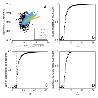
Figure 1: Analysis of networks composed of two subgroups of size $N=1024$. Average internal and external degrees are chosen such that their sum is $\Sigma=\langle k_{in}\rangle+\langle k_{out}\rangle=64$. In- and out-degree sequences are neutrally correlated in the sense that the correlation term of Eq. (5) reads $\xi=\xi_{rand}=\langle k_{in}\rangle\langle k_{out}\rangle$. A Numerical validation of the ansatz of Eq. (3). Please note that here we are showing only the components of the eigenvector $\mathbf{v}_{2}$ that correspond to nodes of one of the two subgroups. Different colors and symbols correspond to different choices of the difference $\Delta=\langle k_{in}\rangle-\langle k_{out}\rangle$. B Linear correlation coefficient between the r.h.s. of Eq. (3) and the numerical estimation of the components of $\mathbf{v}_{2}$ as a function of $\Delta$. C Sum of the components of $\mathbf{v}_{2}$ as a function of $\Delta$. Only the components corresponding to nodes of a single group are considered. This sum is further divided by $\sqrt{N/2}$ in order to obtain a number between zero and one. D Fraction of correctly classified nodes as a function of $\Delta$. In panels B, C and D, the dashed lines stand for the prediction of the detectability threshold $\Delta_{c}=\sqrt{\Sigma}$ [Eq. (7)].

Following the same lines of the approach described in Radicchi (2013, 2014), it is possible to show that the presence of modular structure is revealed by an eigenvector whose $i$-th component behaves, on average, as

$$v^{*}_{i}=q_{i}\,\frac{k_{i}^{in}-k_{i}^{out}}{\sqrt{k_{i}^{in}+k_{i}^{out}}}\;,$$ (3)

with $q_{i}=\pm q$ if node $i$ belongs to the first subgroup, $q_{i}=\mp q$ otherwise, and $q$ proper normalization constant. The validity of the previous approximation can be determined by a direct comparison between the components of the second smallest eigenvector $\mathbf{v}_{2}$ obtained in numerical experiments and the r.h.s. of Eq. (3), as shown for example in Fig. 1A. Using $\mathbf{v}^{*}$ as ansatz in the eigenvalue problem $\mathcal{L}\mathbf{v}^{*}=\nu^{*}\mathbf{v}^{*}$, it is possible to further determine the associated eigenvalue as

$$\nu^{*}=1-\frac{\langle k_{in}^{2}\rangle+\langle k_{out}^{2}\rangle-2\xi}{\langle k_{in}^{2}\rangle-\langle k_{out}^{2}\rangle}\;.$$ (4)

In Eq. (4), $\langle k_{in}^{2}\rangle$ and $\langle k_{out}^{2}\rangle$ are the second moments of the in- and out-degree distributions of the two groups (for Poisson distributions, we have $\langle k_{in}^{2}\rangle=\langle k_{in}\rangle^{2}+\langle k_{in}\rangle$ and $\langle k_{out}^{2}\rangle=\langle k_{out}\rangle^{2}+\langle k_{out}\rangle$), while $\xi$, defined as

$$\xi=\sum_{k^{in},k^{out}}k^{in}k^{out}\,P(k^{in},k^{out})\;,$$ (5)

with $P(k^{in},k^{out})$ probability to find a node with internal and external degrees respectively equal to $k^{in}$ and $k^{out}$, represents the correlation between the number of internal and external connections of the nodes in the network. Please note that the correlation term $\xi$ can be regulated by simply permuting the entries of the in- and out-degree sequences, and thus without changing the correspondent distributions.

In order to determine the detectability threshold, we have to understand whether $\nu^{*}$ effectively represents the second smallest eigenvalue $\nu_{2}$ of $\mathcal{L}$. If this is true then communities are detectable in terms of the components of the eigenvector $\mathbf{v}^{*}=\mathbf{v}_{2}$ defined in Eq. (3), otherwise they are not. The term of comparison of $\nu^{*}$ is given by the expected value $\nu_{rand}$ of the second smallest eigenvalue of the normalized laplacian of a random network with the same average degree $\Sigma=\langle k_{in}\rangle+\langle k_{out}\rangle$, whose value can be estimated, thanks to the predictions by Chung and collaborators Chung et al. (2003a, b), as

$$\nu_{rand}\simeq 1-\frac{2}{\sqrt{\langle k_{in}\rangle+\langle k_{out}\rangle}}\;.$$ (6)

If $\nu^{*}<\nu_{rand}$, this means that $\nu_{2}=\nu^{*}$ and the conditions to reveal the presence of two subgroups are satisfied. If instead $\nu^{*}>\nu_{rand}$, then $\nu_{2}=\nu_{rand}$, and the two subgroups are not detectable by means of the components of the second smallest eigenvector of the normalized laplacian. The condition $\nu^{*}=\nu_{rand}$ determines the detectability threshold $\Delta_{c}$, i.e., the minimal value of the difference $\Delta=\langle k_{in}\rangle-\langle k_{out}\rangle$ for which $\nu^{*}$ equals the typical second smallest eigenvalue $\nu_{rand}$ of a random graph with identical average degree $\Sigma$. As a direct comparison between Eqs. (4) and (6) reveals, the value of $\Delta_{c}$ does not depend only on the average values of internal and external degrees, but also on the correlation term $\xi$ defined in Eq. (5). In the following, we consider three special cases.

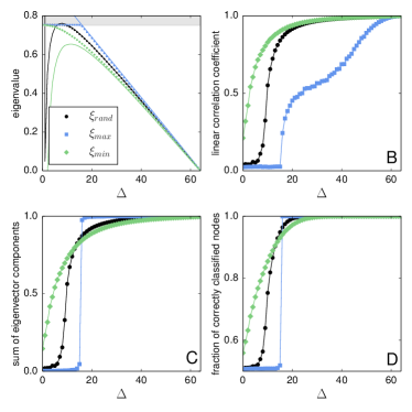
Figure 2: Analysis of networks composed of two subgroups of size $N=1024$. Average internal and external degrees are chosen such that their sum is $\Sigma=\langle k_{in}\rangle+\langle k_{out}\rangle=64$. Different colors and symbols correspond to the three different values of the correlation term $\xi$ described in the text: $\xi_{min}$ (green diamonds), $\xi_{rand}$ (black circles), $\xi_{max}$ (blue squares). All numerical results shown here correspond to average values obtained in 100 realizations of the network models. A Numerical estimation of the second smallest eigenvalue $\nu_{2}$ (symbols). Full lines are obtained with Eq. (4). The gray area delimits the expected spectral radius of the normalized laplacian of a random graph with identical average degree [i.e., Eq. (6)]. B Linear correlation coefficient between the components of $\mathbf{v}_{2}$ and the r.h.s. of Eq. (3) as a function of $\Delta=\langle k_{in}\rangle-\langle k_{out}\rangle$. Only the components of $\mathbf{v}_{2}$ corresponding to nodes of one of the subgroups are considered. C Sum of the components of $\mathbf{v}_{2}$ corresponding to nodes of one of the two subgroups as a function of $\Delta$. To generate numbers between zero and one, this sum is divided by the constant factor $\sqrt{N/2}$. D Fraction of nodes correctly classified as a function of $\Delta$.

Neutrally correlated degree sequences. This is the case usually considered in literature for the determination of the detectability threshold. In- and out-degrees are considered as independent variables, so that the correlation term reads $\xi=\xi_{rand}=\langle k_{in}\rangle\langle k_{out}\rangle$. By equating the r.h.s. of Eqs. (4) and (6), using the definition of the second moments of Poisson distributions, and assuming $\Sigma\gg 1$, we recover the well known result

$$\Delta_{c}=\sqrt{\Sigma}\;.$$ (7)

Such prediction is in perfect agreement with the results of numerical experiments as reported in Figs. 1 and 2. To monitor the transition between the undetectable and detectable regimes, we use three different order parameters: (i) The absolute value of the linear correlation coefficient between the components of the eigenvector $\mathbf{v}_{2}$ (numerically estimated) and the r.h.s. of Eq. (3). Please note that in the evaluation of the linear correlation coefficient we consider only the first $N$ components of $\mathbf{v}_{2}$, i.e., the components corresponding to nodes inside the first subgroup. (ii) The absolute value of the sum of the components of the eigenvector $\mathbf{v}_{2}$ corresponding to nodes within the first subgroup. For convenience, this sum is further divided by the factor $\sqrt{N/2}$ to obtain numbers between zero and one. (iii) Fraction of nodes correctly classified. We consider the classification provided by the signs of the components of the eigenvector $\mathbf{v}_{2}$ and compare it with the pre-imposed division in two subgroups. All the three order parameters clearly show the presence of a transition, as a function of $\Delta$, between a regime in which the modules identified by the spectral algorithm do not correspond to the pre-imposed subgroups, and a regime in which the detected communities coincide instead with them. More importantly, the value of $\Delta$ for which such transition occurs is well approximated by Eq. (7). In intuitive terms, one could try to justify the detectability threshold of Eq. (7) with the following argument. The fact that internal and external degrees are independent variables allows for the presence of nodes whose internal degree is lower than their external number connections even for $\Delta>0$. The assignment to a specific group of nodes with more external than internal connections is technically incorrect, and the second smallest eigenvector of $\mathcal{L}$ provides indeed the right answer by “misplacing” these nodes. Actually, the difference between internal and external node degrees is a random variate that obeys the so-called Skellam distribution with mean equal to $\Delta$ and standard deviation equal to $\sqrt{\Sigma}$ Skellam (1946). Thus, the second smallest eigenvector of $\mathcal{L}$ starts to classify nodes in the pre-imposed subgroups only when the average value of the difference between internal and external degrees is larger than the typical variability of the same variable. This straightforward interpretation is, however, contradicted by the following cases.

Positively correlated degree sequences. If we sort the entries of both internal and external degree sequences in ascending (descending) order, then nodes with high internal degree have high external degree, and vice versa. The re-arrangement inequality tells us that the correlation term reads $\xi=\xi_{max}$, being $\xi_{max}$ the maximum value of $\xi$ that can be reached for fixed entries in the degree sequences Darćzy (1973). Please note that in this case the subgroups in our graph are “well-defined” communities. Apart for extreme cases, we expect in fact that each node in the network have more internal than external connections for every choice of $\Delta>0$. According to the intuitive argument used to justify Eq. (7), we expect to see a detectability threshold not only smaller than the one given in Eq. (7), but also very close to zero. Contrary to intuition, however, the detectability threshold becomes larger (see Fig. 2). Although we cannot provide an exact estimation of $\Delta_{c}$ because we are not able to analytically determine the value of $\xi_{max}$, we can anyway see from our Eq. (4) why this counterintuitive behavior is indeed expected. As $\xi$ increases in fact, the r.h.s. of Eq. (4) gets closer to the typical second smallest eigenvalue of a random graph with average degree $\Sigma$ [i.e., Eq. (6)]. We thus require large values of $\Delta$ in order to make $\nu^{*}$ sufficiently small.

Negatively correlated degree sequences. If we sort the entries of the internal degree sequence in ascending (descending) order, and those of the external degree sequence in descending (ascending) order, then nodes with high internal degree have low external degree, and vice versa. In this case, the re-arrangement inequality states that the correlation term reads $\xi=\xi_{min}$, being $\xi_{min}$ the minimal value of $\xi$ that can be reached for fixed entries in the degree sequences Darćzy (1973). This is the antithetic case of the one just presented for positively correlated degree sequences: even for large values of $\Delta$, the pre-imposed subgroups are “ill-defined” communities, in the sense that it is very likely to find nodes with external degree larger their internal degree. We should thus expect a very large detectability threshold, but again this is expectation is violated. The r.h.s. of Eq. (4) decreases as $\xi$ decreases, so that we require smaller values of $\Delta$ to make $\nu^{*}$ smaller than $\nu_{rand}$. Although in this case, our prediction of Eq. (4) fails to correctly describe the behavior of the second smallest eigenvalue of the normalized laplacian (see Fig. 2), our numerical computations show that $\Delta_{c}=0$, and thus communities are always detectable if $\langle k_{in}\rangle>\langle k_{out}\rangle$.

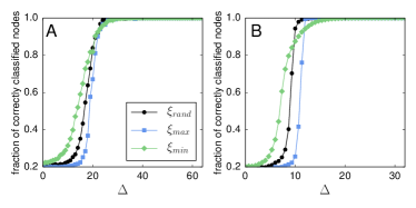
Figure 3: Application of the algorithm by Blondel et al. to the detection of communities in our network block model Blondel et al. (2008). We plot the fraction of nodes that the algorithm correctly classifies as a function of $\Delta=\langle k^{in}\rangle-\langle k^{out}\rangle$. Different colors and symbols correspond to different choices of $\xi$. Each point represents the average performance of the algorithm in $100$ realizations of the model. A Block model composed of two subgroups of size $N=1024$ and average degree $\Sigma=\langle k^{in}\rangle+\langle k^{out}\rangle=64$. B Block model composed of four subgroups of size $N=512$ and average degree $\Sigma=\langle k^{in}\rangle+3\langle k^{out}\rangle=32$.

To summarize, the ability of algorithms to identify communities in networks is dependent on their intrinsic quality. We use the word “quality” in relation with the intuitive notion of communities, and thus on the comparison between the number of internal and external connections at the node level. A “well-defined” community is a subgroup in which each node has more connections with other nodes inside the community than with vertices outside of it, whereas an “ill-defined” community is a subgroup in which many nodes have more connections outside than inside the community. Intuitively, we should expect that good communities are less challenging to be identified than bad communities, but our results show the exact contrary. This situation is paradoxical in the sense that community detection algorithms are developed with the aim of detecting particular kind of substructures, but, in reality, they are better suited to detect groups of nodes that do not fully respect the intuitive definition of communities. One could argue that our results are not general enough because they are based on the performance of a special type of algorithm that is “forced” to classify nodes in two modules, and the random block model on which this algorithm is applied is also composed of two subgroups. These, however, do not seem serious limitations. In Fig. 3, we report the results obtained with the popular community detection algorithm by Blondel et al. Blondel et al. (2008). It is important to stress that this algorithm does not use any previous knowledge regarding the number of subgroups pre-imposed in our block model. Its performances are in line with what shown so far for spectral algorithms: the detection of well-defined communities is more challenging than the identification of ill-defined communities. This is not only valid for the case of two subgroups (Fig. 3A), but applies also to higher numbers of subgroups (Fig. 3B). Although this additional analysis gives a more general character to our results, we do not exclude the presence of other factors that can have an influence on the behavior of the detectability threshold, as for example heterogeneous community sizes and/or node degrees. Accounting for other relevant effects surely represents the next step towards a deeper understanding of this appealing and important problem. Also, in the search of possible resolutions of the paradoxical situation illustrated in this paper, our results indicates a promising direction to explore: the numerator $\langle(k_{in}-k_{out})^{2}\rangle=\langle k_{in}^{2}\rangle+\langle k_{out}^{2}\rangle-2\xi$ of the fraction appearing in Eq. (4) suggests that the second moment of the distribution of the variables $k_{in}-k_{out}$ play a role as important as its first moment in the determination of the detectability threshold. We believe that this information can be used to redesign the mechanisms at the basis of community detection algorithms.

As a final remark, we would like to stress that the relevance of our results is not only theoretical, but also practical. Consider for example the case of artificial graphs used to test the performance of community detection algorithms Danon et al. (2005); Lancichinetti and Fortunato (2009). These are typically constructed on the basis of random block models very similar to the one considered in this paper. However, depending on the particular recipe used to construct them, the correlation between internal and external degrees at the node level can be very different. As paradigmatic examples, consider the two benchmark graphs that are widely adopted for testing the performance of community detection algorithms: the Girvan-Newman (GN) and the Lancichinetti-Fortunato-Radicchi (LFR) benchmark graphs Girvan and Newman (2002); Lancichinetti et al. (2008). The LFR model is generally considered the extension of the GN model to heterogeneous node degrees and community sizes, but this is not totally correct. In the GN model, internal and external degrees are neutrally correlated; on contrary in the LFR graphs, internal and external degrees are positively correlated. Comparisons in the performance of community identification methods across these two benchmark models are thus not possible, and this is a fundamental consideration to take into account when choosing the best algorithm to detect a priori unknown clusters in real networks.