$2D$ and $3D$ Antiferromagnetic Ising Model with ”topological” term at $\theta=\pi$

Abstract:

We study the two and three-dimensional Antiferromagnetic Ising Model with an imaginary magnetic field $i\theta$ at $\theta=\pi$. We use a new geometric algorithm which does not present a sign problem. This allows us to perform efficient numerical simulations of this system.

1 Introduction

Numerical simulations are one of the main tools that allow us to obtain quantitative results in many fields of physics, and they have played an essential part in the progress of QCD and condensed matter physics in recent years. There are, however, many interesting physical systems for which we do not have efficient numerical algorithms yet. Examples include QCD at finite density or with a non-vanishing $\theta$ term. This situation has hindered progress in such fields for a long time, and it is thus of great interest to study novel simulation algorithms.

In the present work we develop and test a geometric algorithm which we apply to study the two-dimensional antiferromagnetic Ising model with an imaginary magnetic field i$\theta$ (see [1], [2] and [3]) at $\theta=\pi$ [4], and which solves the sign problem that this model has when using standard algorithms. In this work also the $3D$ model is studied.

2 The model and a geometric algorithm

We start with the (reduced) Hamiltonian for the Ising model in $D\geq 2$ in an external magnetic field,

$$H(\{s_{x}\},F,h)=-F\sum_{(x,y)\in{\cal B}}s_{x}s_{y}-\frac{h}{2}\sum_{x}s_{x}\,.$$ (1)

We consider a $D$-dimensional hypercubic lattice with $L=2n\in\mathbb{N}$ sites by side, and we denote the lattice sites by $x$ and the spin variables with $s_{x}\in\{\pm 1\}$. The sum $\sum_{(x,y)\in{\cal B}}$ runs over the set ${\cal B}$ of all nearest-neighbors $(x,y)$; $F=J/(k_{B}T)$ is the reduced coupling between spins, and $h=2B/(k_{B}T)$, with $B$ the external magnetic field. The total number of spins is $V=L^{D}=(2n)^{D}$, thus even, and therefore the quantity $Q\equiv\frac{1}{2}\sum_{x}s_{x}$ is an integer number, taking values between $-L^{D}/2$ and $L^{D}/2$, which can be thought of as playing the role of a topological charge. We are interested in studying this system for imaginary values of the reduced magnetic field $h$, i.e., for $h=i\theta$.

This model suffers from a sign problem, because the weight of a configuration is not a positive real number, and therefore we cannot apply a standard algorithm. For the special case $\theta=\pi$ we will show how to construct an efficient geometric algorithm that circumvents this problem.

The partition function of the system at $\theta=\pi$ is

$$Z(F,\theta=\pi)=\sum_{\{s_{x}=\pm 1\}}e^{F\sum_{(x,y)\in{\cal B}}s_{x}s_{y}+i\frac{\pi}{2}\sum_{z}s_{z}}$$ (2)

$$=i^{V}\sum_{\{s_{x}=\pm 1\}}\left\{\prod_{(x,y)\in{\cal B}}[\cosh(Fs_{x}s_{y})+\sinh(Fs_{x}s_{y})]\prod_{z}{s_{z}}\right\}$$

$$=\sum_{\{s_{x}=\pm 1\}}\left\{\prod_{(x,y)\in{\cal B}}[\cosh(F)+\sinh(F)s_{x}s_{y}]\prod_{z}{s_{z}}\right\}\,.$$

It is easy to see, by decomposing the lattice in two staggered sublattices, that $Z(F,\pi)=Z(-F,\pi)$; therefore, at $\theta=\pi$, the ferromagnetic and antiferromagnetic models are equivalent, and furthermore $Z$ is in fact a function of $|F|$.

We can now expand the product inside the curly brackets, and assign a unique graph to each term in the expansion: to each factor $\sinh(|F|)s_{x}s_{y}$ we assign the bond $(x,y)\in{\cal B}$ in the graph, and we say that such a bond is active. Every other bond is called inactive, and corresponds to a factor $\cosh(|F|)$. Each set of active bonds describes one and only one of the terms in the expansion. After summing over spin states most of the contributions in the expansion vanish; only the graphs such that every node on the lattice has an odd number of active bonds touching it give a non-vanishing contribution. We call such graphs admissible, and we denote by ${\cal G}$ the set of all admissible graphs. If we consider an admissible graph, $g\in{\cal G}$, and denote by ${\cal N}_{b}(g)$ the number of active bonds in $g$, by $\bar{\cal N}_{b}(g)$ the number of inactive bonds in $g$, and by ${\cal N}$ the total number of bonds in the lattice (thus ${\cal N}={\cal N}_{b}(g)+\bar{\cal N}_{b}(g)$), the weight of such graph in the partition function is $2^{V}\sinh(|F|)^{{\cal N}_{b}(g)}\cosh(|F|)^{\bar{\cal N}_{b}(g)}$. Therefore we can rewrite the partition function as:

$$Z(F,\theta=\pi) =2^{V}\sum_{\begin{subarray}{c}g\in{\cal G}\end{subarray}}\cosh(|F|)^{{\bar{\cal N}}_{b}(g)}\sinh(|F|)^{{\cal N}_{b}(g)}$$ (3)

$$=2^{V}\cosh(|F|)^{{\cal N}}\sum_{\begin{subarray}{c}g\in{\cal G}\end{subarray}}\tanh(|F|)^{{\cal N}_{b}(g)}\,.$$

The important point here is that all configurations (graphs) have positive weights, and therefore this representation of the partition function does not have a sign problem. Now, generalizing the partition function (3) to the case where the coupling is position-dependent, we obtain:

$$Z(\{F_{xy}\},\theta=\pi)=\sum_{\{s_{x}=\pm 1\}}\left\{\prod_{(x,y)\in{\cal B}}[\cosh(|F_{xy}|)+\sinh(|F_{xy}|)s_{x}s_{y}]\prod_{z}{s_{z}}\right\}\,.$$ (4)

From this expression we are able to build all the correlation functions for an even number of spins (correlation functions with an odd number of spins are automatically zero). After some calculations (see [5]) we obtain the following expression for the correlation functions:

$$C(d,F)\equiv\langle s_{x}s_{x+d\hat{1}}\rangle=\left[\prod_{i=1}^{d}\frac{\partial}{\partial F_{x_{i}x_{i+1}}}\right]\log Z(\{F_{xy}\},\theta=\pi)\bigg{|}_{\{F_{xy}\}=\{F\}}\\ =\langle\!\langle\tanh(F)^{d-2{\cal N}_{b}[g,\{x_{i},y_{i}\}]}\rangle\!\rangle\,,$$ (5)

where ${\cal N}_{b}[g,\{x_{i},y_{i}\}]$ is the number of active bonds along the straight path connecting $x$ and $x+d\hat{1}$. However, we stress the fact that the specific choice of the path is irrelevant, as they are all equivalent, as long as the endpoints are fixed. It is also possible to obtain the relations for the energy density and specific heat by taking derivatives of the partition function with respect to the coupling constant. In fact, using our geometric algorithm these observables are related to the average number of active bonds and its fluctuations (the details of the derivation of these expressions will be discussed in [5]).

3 Simulation

In order to perform calculations using Monte Carlo methods, we need an efficient algorithm to explore the space of configurations, that in the geometric representation is given by the set of admissible graphs, ${\cal G}$. The essential ingredient is a local prescription that takes the system from an admissible configuration to another admissible configuration. The simplest change that one can do to a configuration is to make an inactive bond into an active one, or viceversa. However, applying this change to an admissible configuration will not take us to another admissible configuration. Let us consider instead an arbitrary square on the lattice, and consider all possible changes in the state of the bonds in the square. It is easy to convince oneself that if we start from an admissible configuration, the only way to arrive at another admissible configuration is either by not changing the state of any of the bonds, or by changing all of them. Using these steps and the weights of the configurations derived above, it is now easy to set up a standard Metropolis algorithm.

We measured how the correlation functions (5) depends on the distance $d$, choosing different antiferromagnetic couplings $F<0$ and varying the lattice volume $V=L^{D}$, in order to determine the staggered magnetization from their asymptotic behavior. In Figs. (1) we present some results concerning the evaluation of these correlation functions for different values of the coupling $F$ and various lattice sizes ranging from $L=64$ to $L=1024$ both for the $2D$ model and the $3D$ model. Simulations are done collecting 100k measurements for each value of $F$. For each run we discarded the first 10k configurations in order to ensure thermalization. The jackknife method over bins at different blocking levels was used for the data analysis.

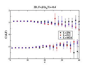
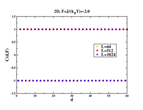
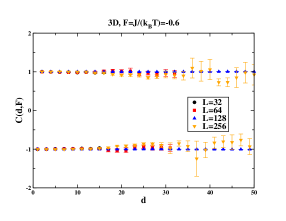
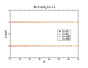
Figure 1: Dependence of the correlation functions on the distance $d$ for some values of the coupling $F$ and for various lattice sizes $L$ for the $2D$ model (top) and the $3D$ model (bottom).

For antiferromagnetic couplings, the behavior of the correlation functions implies that the staggered magnetization is nonzero, while the total magnetization vanishes, in the whole range of couplings that we investigated. This result is in agreement with Refs. [1, 2, 3], and with the mean-field calculation of Ref. [6]. The apparent decrease of $C(d,F)$, starting from $d\sim 10\div 20$, for small values of $|F|$, is probably due to the heavy-tailed probability distributions of the correlators, which is also the cause of their noisy behavior. In Fig. 3 we show the probability distributions of the logarithm of the correlators for lattice size $L=64$ and $F=-0.4$ and $F=-2.0$. We can clearly see that for a small coupling $|F|$ the values are spread in a wider range than for $F=-2.0$, and also that a long tail is developed for large distances. This makes more difficult to obtain an accurate numerical evaluation of the correlators. In Fig. (2) we show also the behavior of the energy density and of the specific heat for both the $2D$ model and the $3D$ model signalling that no phase transitions occur. More details, also concerning the proof of the ergodicity of the algorithm, will be presented in [5].

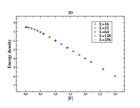
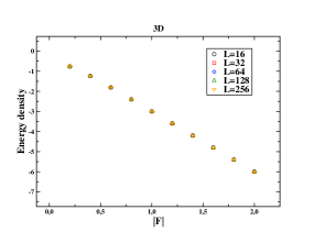
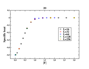
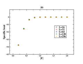
Figure 2: Energy density as a function of $|F|$ for various lattice sizes $L$ for the $2D$ model (top left) and the $3D$ model (top right); specific heat as a function of $|F|$ for the $2D$ model (bottom left) and the $3D$ model (bottom right).

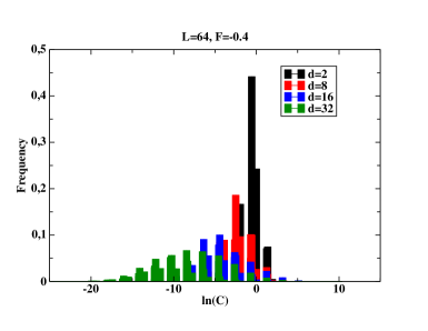
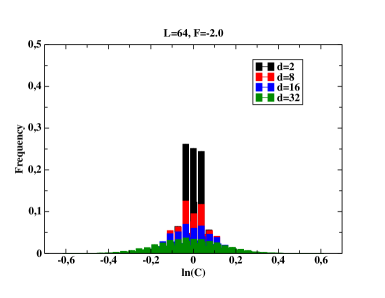
Figure 3: Probability distribution of the logarithm of the correlator $C(d,F)$ for various distances $d$, for a lattice of size $L=64$, and for coupling $F=-0.4$ (top) and $F=-2.0$ (bottom). The figures depicted here are obtained for the $2D$ model.

- [1] T. D. Lee and C. N. Yang, Phys. Rev. 87 (1952) 410.
- [2] V. Matveev and R. Shrock, J. Phys. A 28 (1995) 4859.
- [3] B. M. McCoy and T. T. Wu, Phys. Rev. 155 (1967) 438.
- [4] V. Azcoiti, G. Cortese, E. Follana, and M. Giordano, PoS LATTICE 2012 (2012) 248.
- [5] V. Azcoiti, G. Cortese, E. Follana, and M. Giordano, in preparation.
- [6] V. Azcoiti, E. Follana, and A. Vaquero, Nucl. Phys. B 851 (2011) 420.