Robust EM algorithm for model-based curve clustering

Abstract

Model-based clustering approaches concern the paradigm of exploratory data analysis relying on the finite mixture model to automatically find a latent structure governing observed data. They are one of the most popular and successful approaches in cluster analysis. The mixture density estimation is generally performed by maximizing the observed-data log-likelihood by using the expectation-maximization (EM) algorithm. However, it is well-known that the EM algorithm initialization is crucial. In addition, the standard EM algorithm requires the number of clusters to be known a priori. Some solutions have been provided in [31, 12] for model-based clustering with Gaussian mixture models for multivariate data. In this paper we focus on model-based curve clustering approaches, when the data are curves rather than vectorial data, based on regression mixtures. We propose a new robust EM algorithm for clustering curves. We extend the model-based clustering approach presented in [31] for Gaussian mixture models, to the case of curve clustering by regression mixtures, including polynomial regression mixtures as well as spline or B-spline regressions mixtures. Our approach both handles the problem of initialization and the one of choosing the optimal number of clusters as the EM learning proceeds, rather than in a two-fold scheme. This is achieved by optimizing a penalized log-likelihood criterion. A simulation study confirms the potential benefit of the proposed algorithm in terms of robustness regarding initialization and funding the actual number of clusters.

I Introduction

Clustering approaches concern the paradigm of exploratory data analysis in which we aim at automatically finding a latent structure within an observed dataset through which the data can be summarized in a few number of clusters. From a statistical learning prospective, cluster analysis involves unsupervised learning techniques, in the sense that the class labels of the data are unknown (missing, hidden or difficult to obtain), to learn an underlying structure of the latent data governing the observed data. This is generally performed through learning the parameters of a latent variable model. Clustering techniques are therefore suitable for many application domains where labeled data is difficult to obtain, or to explore and characterize a dataset before running a supervised learning algorithm, etc. The aim of clustering in general is to find a partition of the data by dividing them into clusters (groups) such that the data within the same group tend to be more similar, in the sense of a chosen dissimilarity measure, to one another as compared to the data belonging to different groups. The definition of (dis)similarity and the method in which the data are clustered differs based on the clustering algorithm being applied. One can distinguish four categories of clustering algorithms: hierarchical clustering, distance-based (or prototype-based) clustering, topographic clustering and model-based clustering. Hierarchical clustering [17] aims at building a hierarchy of clusters and includes ascending (or agglomerative) hierarchical clustering and descending (or splitting) hierarchical clustering. In the former, each data example starts in its own cluster, and pairs of clusters are successively merged as one moves up the hierarchy. The pair of clusters to be merged is chosen as the pair of closest clusters in the sense of a chosen distance criterion (e.g. Ward distance, etc). The latter approach operates in the other sense. Among one of the most known prototype-based clustering algorithms, one can cite the $K$-means algorithm [22, 16]. $K$-means is a straightforward and widely used algorithm in cluster analysis. It is an iterative clustering algorithm that partitions a given dataset into a predefined number of clusters $K$ by minimizing the within-cluster variance criterion (intra-class inertia). Several variants of $K$-means, including fuzzy $K$-means [2], trimmed $K$-means [10, 15], etc, have been proposed. One of the most popular topographic clustering approaches is the Self Organizing Map [20]. The SOM is an unsupervised neural-based approach for data clustering and visualization. It generalizes the competitive learning [21] by allowing also the neighbours of the winner to be updated. This is performed by minimizing a cost function (distance criterion) taking into account the topological aspect of the data through a neighborhood kernel (e.g. Gaussian). These clustering approaches can be seen as deterministic as they do not define a density model on the data. When the clustering approaches rely on density modeling, clustering is generally performed based on the finite mixture model [24]. This approach is known as the model-based clustering [1, 25, 13]. Mixture model-based approaches are indeed one of the most popular and successful unsupervised learning approaches in cluster analysis. In the finite mixture approach for cluster analysis, the data probability density function is assumed to be a mixture density, each component density being associated with a cluster. The problem of clustering therefore becomes the one of estimating the parameters of the assumed mixture model (e.g, estimating the mean vector and the covariance matrix for each component density in the case of Gaussian mixture models). The mixture density estimation is generally performed by maximizing the observed data log-likelihood. This can be achieved by the well-known expectation-maximization (EM) algorithm [11, 23]. The EM algorithm is in the core of these model-based clustering approaches thanks to its good desirable properties of stability and reliable convergence. The EM algorithm is indeed a broadly applicable approach to the iterative computation of maximum likelihood estimates in the framework of latent data models and in particular in finite mixture models. It has a number of advantages, including its numerical stability, simplicity of implementation and reliable convergence. For more account on EM, the reader is referred to [23]. Furthermore, model-based clustering indeed provides a more general well-established probabilistic framework for cluster analysis compared to deterministic clustering algorithms such as $K$-means algorithms, SOM algorithms, etc. For example it has been shown that from a probabilistic point of view, $K$-means is equivalent to a particular case of the Classification EM (CEM) algorithm [6] for a mixture of $K$ Gaussian densities with the same mixing proportions and identical isotropic covariance matrices. The generative version of the Self Organizing Map, that is the Generative Topographic Mapping [4], allows to overcome the SOM limitations through the probabilistic formulation of a latent variable where both convergence and topographic ordering are guaranteed thanks to the good properties of the EM algorithm. For all these approaches, the choice of the number of classes can be performed afterwards the learning process. For example, in model-based clustering, one can use some information criteria for model selection, such as BIC [30], etc, in order to estimate the optimal number of clusters.

In this paper we focus on model-based clustering approaches, in particular model-based curve clustering based on regressions mixtures. Indeed, the main model-based clustering approaches are concerned with vectorial data where the observations are vectors of reduced dimension and the clustering is performed by Gaussian mixture models and the EM algorithm [24, 23, 31]. Each cluster is represented by its mean vector and its covariance matrix. In many areas of application, the data are curves or functions rather than vectors. The analysis approaches are therefore linked to Functional Data Analysis (FDA) [26] Statistical approaches for FDA [26] concern the paradigm of data analysis for which the individuals are entire functions or curves rather than vectors of reduced dimensions. The goals of FDA, as in classical data analysis, include data representation, regression, classification, clustering, etc. From a statistical learning prospective of FDA, the curve clustering can be achieved by learning adapted statistical models, in particular latent data models, in an unsupervised context. When the observations are curves or time series, the clustering can therefore be performed model-based curve clustering approaches, namely the regression mixture model [14, 7]. including polynomial regression mixtures, splines and B-splines regression mixtures [14, 7], or also generative polynomial piecewise regression [29, 7, 8], The parameter estimation is still performed by maximizing the observed-data log-likelihood through the EM algorithm. However, it is well-known that, for Gaussian mixtures as well as for regression mixtures, the initialization of the EM algorithm is a crucial point since it maximizes locally the log-likelihood. Therefore, if the initial value is inappropriately selected, the EM algorithm may lead to an unsatisfactory estimation. In addition, the standard EM algorithm requires the number of clusters to be known which is not always the case. Choosing the optimal number of clusters can be performed afterwards using some information criteria such as the Bayesian information criterion (BIC) [30], etc.

In this paper we focus on model-based curve clustering using regressions mixtures. We consider the problem of curve clustering where the observations are temporal curves rathen than vectors as in multivariate Gaussian mixture analysis [31]. We extend the model-based clustering approach presented in [31], in which a robust EM is developed for Gaussian mixture models, to the case of regression mixtures, including spline regression mixtures or B-spline regression mixtures for curve clustering. More specifically, we propose a new robust EM clustering algorithm for regressions mixtures, which can be used for polynomial regression mixture as well as for spline or B-spline regressions mixtures. Our approach handles both the problem of initialization and the one of choosing the optimal number of clusters as the EM learning proceeds, rather that in a two-fold scheme. The approach allows therefore for fitting regression mixture models without running an external algorithm for initializing the EM algorithm and without specifying the number of the clusters in the dataset a prior or performing a model selection procedure once the learning has been performed. We mainly focus on generative approaches which may help us to understand the process generating the curves. The generative approaches for functional data are essentially based on regression analysis, including polynomial regression, splines and B-splines [14, 7].

This paper is organized as follows. In the next sections we give a brief background on model-based clustering of multivariate data using Gaussian mixtures and model-based curve clustering using regression mixtures. Then, in section IV we present the proposed robust EM algorithm which maximizes a penalized log-likelihood criterion for regression mixture model-based curve clustering. and derive the corresponding parameter updating formulas.

II Background on model-based clustering with Gaussian mixtures

In this section, we give a brief background on model-based clustering of multivariate data using Gaussian mixtures. Model-based clustering [1, 25, 13], generally used for multidimensional data, is based on a finite mixture model formulation [24].

Let us denote by $(\mathbf{x}_{1},\ldots,\mathbf{x}_{n})$ an observed i.i.d dataset, each observation $\mathbf{x}_{i}$ is represented as multidimensional vector in $\mathbb{R}^{d}$. We let also $\mathbf{z}=(z_{1},\ldots,z_{n})$ denotes the corresponding unobserved (missing) labels where the class label $z_{i}$ takes its values in the finite set $\{1,\ldots,K\}$, $K$ being the number of clusters. In the finite mixture model, the data probability density function is assumed to be a Gaussian mixture density defined as

$$f(\mathbf{x}_{i};\boldsymbol{\Psi})=\sum_{k=1}^{K}\pi_{k}\mathcal{N}\big{(}\mathbf{x}_{i};\boldsymbol{\mu}_{k},\boldsymbol{\Sigma}_{k}\big{)},$$ (1)

each component Gaussian density being associated with a cluster. $\mathcal{N}(.;\boldsymbol{\mu},\boldsymbol{\Sigma})$ denotes the multivariate Gaussian density with mean vector $\boldsymbol{\mu}$ and covariance matrix $\boldsymbol{\Sigma}$. In this mixture density, the $\pi_{k}$’s are the non-negative mixing proportions that sum to 1 and $\boldsymbol{\mu}_{k}$ and $\boldsymbol{\Sigma}_{k}$ are respectively the mean vector and the covariance matrix for each mixture component density. The problem of clustering therefore becomes the one of estimating the parameters of the Gaussian mixture model $\boldsymbol{\Psi}=(\pi_{1},\ldots,\pi_{K},\boldsymbol{\Psi}_{1},\ldots,\boldsymbol{\Psi}_{K})$ where $\boldsymbol{\Psi}_{k}=(\boldsymbol{\mu}_{k},\boldsymbol{\Sigma}_{k})$. This can be performed by maximizing the following observed-data log-likelihood of $\boldsymbol{\Psi}$ by using the EM algorithm [23, 11]:

$$\mathcal{L}(\boldsymbol{\Psi})=\sum_{i=1}^{n}\log\sum_{k=1}^{K}\pi_{k}\mathcal{N}\big{(}\mathbf{x}_{i};\boldsymbol{\mu}_{k},\boldsymbol{\Sigma}_{k}\big{)}.$$ (2)

However, the EM algorithm for Gaussian mixture models is quite sensitive to initial values. The Gaussian mixture model-based clustering technique might yield poor clusters if the mixture parameters are not initialized properly. The EM initialization can be performed from a randomly chosen partition of the data or by computing a partition from another clustering algorithm such as $K$-means, Classification EM [5], Stochastic EM [6], etc or by initializing EM with a few number of steps of EM itself. Several works have been proposed in the literature in order to overcome this drawback and making the EM algorithm for Gaussian mixtures robust with regard initialization [3, 27, 31]. Further details about choosing starting values for the EM algorithm for Gaussian mixtures can be found for example in [3]. On the other hand, the number of mixture components (clusters) needs to be known a priori. Some authors have considered this issue in order to estimate the unknown number of mixture components, for example as in [28, 31]. In general, theses two issues have been considered each separately. Among the approaches considering both the problem of robustness with regard to initial values and automatically estimating the number of mixture components in the same algorithm, one can cite the EM algorithm proposed in [12]. In [12], the authors proposed an EM algorithm that is capable of selecting the number of components and it attempts to be not sensitive with regard to initial values. In deed, the algorithm developed in [12] optimizes a particular criterion called the minimum message length (MML), which is a penalized negative log-likelihood rather than the observed data log-likelihood. The penalization term allows to control the model complexity. Indeed, the EM algorithm in [12] starts by fitting a mixture model with large number of clusters and discards illegitimate clusters as the learning proceeds. The degree of legitimate of each cluster is measured through the penalization term which includes the mixing proportions to know if the cluster is small or not to be discarded and therefore to reduce the number of clusters.

More recently, in [31], the authors developed a robust EM algorithm for model-based clustering of multivariate data using Gaussian mixture models that simultaneously addresses the problem of initialization and estimating the number of mixture components. This algorithm overcome some initialization drawback of the EM algorithm proposed in [12], which is still having an initialization problem. As shwon in [31], this problem can become more serious especially for a dataset with a large number of clusters. For more details on robust EM clustering for Gaussian mixture models for multivariate data, the reader is referred to [31].

However, these presented model-based clustering approaches, namely [31] [12], are concerned with vectorial data where the observations are assumed to be vectors of reduced dimension. When the data are rather curves or functions, one can rely on regression mixtures [14, 7] or generative hidden process regression [9][7] which are more adapted than standard Gaussian mixture modeling.

In the next section we describe the model-based curve clustering approach based on regression mixtures using the standard EM algorithm and then we derived our EM algorithm in the following section.

III Background on model-based curve clustering with regression mixtures

III-A Model-based curve clustering

Mixture-model-based clustering approaches have also been introduced to generalize the standard multivariate mixture model to the analysis of curves where the individuals are presented as curves rather than a vector of a reduced dimension. In this case, one can distinguish the regression mixture approaches, including polynomial regression and spline regression, or random effects polynomial regression [14, 19]. Notice that the mixture of regression models are similar to the well-known mixture of experts (ME) model [18]. Although similar, mixture of experts differ from curve clustering models in many respects (for instance see [14]). One of the main differences is that the ME model consists in a conditional mixture while the mixture of regressions is an unconditional one. Indeed, the mixing proportions are constant for the mixture of regressions, while in the mixture of experts, they mixing proportions (known as the gating functions of the network) are modeled as a function of the inputs, generally as a logistic or a softmax function. All these approaches use the mixture (estimation) approach with the EM algorithm to estimate the model parameters. One can also consider generative hidden process regression mixtures [9][7] [29] which performs curve segmentation.

III-B Regression mixtures for model-based curve clustering

In this section we describe related model-based curve clustering approaches based on regression mixture models [14, 7].

The aim of EM clustering in the case of regression mixtures is to cluster $n$ iid curves $((\mathbf{x}_{1},\mathbf{y}_{1}),\ldots,(\mathbf{x}_{n},\mathbf{y}_{n}))$ into $K$ clusters. We assume that each curve consists of $m$ observations $\mathbf{y}_{i}=(y_{i1},\ldots,y_{im})$ regularly observed at the inputs $\mathbf{x}_{i}=(x_{i1},\ldots,x_{im})$ for all $i=1,\ldots,n$ (e.g., $\mathbf{x}$ may represent the sampling time in a temporal context). Let $\mathbf{z}=(z_{1},\ldots,z_{n})$ be the unknown cluster labels associated with the set of curves (time series) $(\mathbf{y}_{1},\ldots,\mathbf{y}_{n})$, with $z_{i}\in\{1,\ldots,K\}$, $K$ being the number of clusters. The regression mixtures approaches assume that each curve is drawn from one of $K$ clusters of curves whose proportions (prior probabilities) are $(\pi_{1},\ldots,\pi_{K})$. Each cluster of curves is supposed to be a set of homogeneous curves modeled by for example a polynomial regression model or a spline regression model. The polynomial Gaussian regression mixture model arises when we assume that, the curve $(\mathbf{x}_{i},\mathbf{y}_{i})$ has a prior probability $\pi_{k}$ to be generated from the cluster $z_{i}=k$ and is generated according to a noisy polynomial (or spline) function with (polynomial) coefficients $\boldsymbol{\beta}_{k}$ corrupted by a standard zero-mean Gaussian noise with a covariance-matrix $\sigma_{k}^{2}\textbf{I}_{m}$, that is, for the cluster $k$ we have

$$\mathbf{y}_{i}=\mathbf{X}_{i}\boldsymbol{\beta}_{k}+\boldsymbol{\epsilon}_{i}$$ (3)

where $\mathbf{y}_{i}=(y_{i1},\ldots,y_{im})^{T}$ is an $m$ by $1$ vector, $\mathbf{X}_{i}$ is the $m$ by $(p+1)$ regression matrix (Vandermonde matrix) with rows $\boldsymbol{x}_{i}=(1,x_{ij},x_{ij}^{2}\ldots,x_{ij}^{p})$, $p$ being the polynomial degree, $\boldsymbol{\beta}_{k}=(\beta_{k0},\ldots,\beta_{kp})^{T}$ is the $(p+1)$ by $1$ vector of regression coefficients for class $k$, $\boldsymbol{\epsilon}_{i}\sim\mathcal{N}(\mathbf{0},\sigma_{k}^{2}\textbf{I}_{m})$ is a multivariate standard zero-mean Gaussian variable with a variance $\sigma_{k}^{2}\textbf{I}_{m}$, representing the corresponding Gaussian noise and $\textbf{I}_{m}$ denotes the $m$ by $m$ identity matrix. We notice that the regression mixture is adapted for polynomial regression mixture as well as for spline of B-slipne regression mixtures. This only depends on the construction of the regression matrix $\mathbf{X}_{i}$. The conditional density of curves from cluster $k$ is therefore given by

$$f_{k}(\mathbf{y}_{i}|\mathbf{x}_{i},z_{i}=k;\boldsymbol{\beta}_{k},\sigma_{k}^{2})=\mathcal{N}(\mathbf{y}_{i};\mathbf{X}_{i}\boldsymbol{\beta}_{k},\sigma_{k}^{2}\textbf{I}_{m}),$$ (4)

and finally the conditional mixture density of the $i$th curve can be written as:

$$f(\mathbf{y}_{i}|\mathbf{x}_{i};\boldsymbol{\Psi}) = \sum_{k=1}^{K}p(z_{i}=k)f_{k}(\mathbf{y}_{i}|\mathbf{x}_{i},z_{i}=k;\boldsymbol{\beta}_{k},\sigma_{k}^{2})$$ (5)

$$= \sum_{k=1}^{K}\pi_{k}\ \mathcal{N}(\mathbf{y}_{i};\mathbf{X}_{i}\boldsymbol{\beta}_{k},\sigma_{k}^{2}\textbf{I}_{m}).$$

where the model parameters are given by $\boldsymbol{\Psi}=(\pi_{1},\ldots,\pi_{K},\boldsymbol{\Psi}_{1},\ldots,\boldsymbol{\Psi}_{K})$ where the $\pi_{k}$’s are the non-negative mixing proportions that sum to 1 $\boldsymbol{\Psi}_{k}=(\boldsymbol{\beta}_{k},\sigma_{k}^{2})$, $\sigma_{k}^{2}$ represents the regression parameters and the noise variance for cluster $k$. The unknown parameter vector $\boldsymbol{\Psi}$ is generally estimated by maximizing the observed-data log-likelihood of $\boldsymbol{\Psi}$. Given an i.i.d training set of $n$ curves the observed-data log-likelihood of $\boldsymbol{\Psi}$ is given by:

$$\mathcal{L}(\boldsymbol{\Psi})=\sum_{i=1}^{n}\log\sum_{k=1}^{K}\pi_{k}\ \mathcal{N}(\mathbf{y}_{i};\mathbf{X}_{i}\boldsymbol{\beta}_{k},\sigma_{k}^{2}\textbf{I}_{m}).$$ (6)

and its maximization is performed iteratively via the EM algorithm [14, 11, 7].

III-C Standard EM algorithm for regression mixtures

The maximization of the observed-data the log-likelihood (6) by the EM algorithm relies on the complete-data log-likelihood, that is assuming the hidden labels $\mathbf{z}$ are known:

$$\mathcal{L}_{c}(\boldsymbol{\Psi}) = \sum_{i=1}^{n}\sum_{k=1}^{K}z_{ik}\log\big{[}\pi_{k}\mathcal{N}(\mathbf{y}_{i};\mathbf{X}_{i}\boldsymbol{\beta}_{k},\sigma^{2}_{k}\textbf{I}_{m})\big{]}$$ (7)

where $z_{ik}$ is an indicator binary-valued variable such that $z_{ik}=1$ if $z_{i}=k$ (i.e., if $\mathbf{y}_{i}$ is generated by the polynomial regression component $k$) and $z_{ik}=0$ otherwise.

At each iteration, the EM maximizes the expectation of the complete-data log-likelihood (7) given the observed data $\mathcal{D}=((\mathbf{x}_{1},\mathbf{y}_{1}),\ldots,(\mathbf{x}_{n},\mathbf{y}_{n}))$ and a current parameter estimation of $\boldsymbol{\Psi}$. The EM algorithm for regression mixtures therefore starts with an initial model parameters $\boldsymbol{\Psi}^{(0)}$ and alternates between the two following steps until convergence:

III-C1 E-step

Compute the expected complete-data log-likelihood given the observed curves $\mathcal{D}=((\mathbf{x}_{1},\mathbf{y}_{1}),\ldots,(\mathbf{x}_{n},\mathbf{y}_{n}))$ and the current value of the parameter $\boldsymbol{\Psi}$ denoted by $\boldsymbol{\Psi}^{(q)}$, $q$ being the current iteration number:

$$Q(\boldsymbol{\Psi},\boldsymbol{\Psi}^{(q)}) = \mathbb{E}\big{[}\mathcal{L}_{c}(\boldsymbol{\Psi})|\mathcal{D};\boldsymbol{\Psi}^{(q)}\big{]}$$ (8)

$$= \sum_{i=1}^{n}\sum_{k=1}^{K}\tau_{ik}^{(q)}\log\big{[}\pi_{k}\mathcal{N}(\mathbf{y}_{i};\mathbf{X}\boldsymbol{\beta}_{k},\sigma^{2}_{k}\textbf{I}_{m})\big{]}\cdot$$

This simply consists in computing the posterior probability that the $i$th curve is generated from cluster $k$

$$\tau_{ik}^{(q)} = p(z_{i}=k|\mathbf{y}_{i},\mathbf{x}_{i};\boldsymbol{\Psi}^{(q)})$$ (9)

$$= \frac{\pi_{k}^{(q)}\mathcal{N}\big{(}\mathbf{y}_{i};\mathbf{X}_{i}\boldsymbol{\beta}^{(q)}_{k},\sigma^{2(q)}_{k}\textbf{I}_{m}\big{)}}{\sum_{h=1}^{K}\pi_{h}^{(q)}\mathcal{N}(\mathbf{y}_{i};\mathbf{X}_{i}\boldsymbol{\beta}^{(q)}_{h},\sigma^{2(q)}_{h}\textbf{I}_{m})}$$

for each curve and for each of the $K$ clusters.

III-C2 M-step

This step updates the models parameters by computing the update $\boldsymbol{\Psi}^{(q+1)}$ by maximizing the $Q$-function (8) with respect to $\boldsymbol{\Psi}$. The updating formula for the mixing proportion is obtained by maximizing $\sum_{i=1}^{n}\sum_{k=1}^{K}\tau^{(q)}_{ik}\log\pi_{k}$ with respect to $(\pi_{1},\ldots,\pi_{R})$ subject to the constraint $\sum_{k=1}^{K}\pi_{k}=1$ using Lagrange multipliers which gives the following updates [23, 11, 14, 7]

$$\pi_{k}^{(q+1)} = \frac{1}{n}\sum_{i=1}^{n}\tau^{(q)}_{ik}\quad(k=1,\ldots,K).$$ (10)

The maximization of each of the $K$ functions $\sum_{i=1}^{n}\tau_{ik}^{(q)}\log\mathcal{N}(\mathbf{y}_{i};\mathbf{X}\boldsymbol{\beta}_{k},\sigma^{2}_{k}\textbf{I}_{m})$ consists in solving a weighted least-squares problem. The solution of this problem is straightforward and these update equations are equivalent to the well-known weighted least-squares solutions (see for example [14, 7]):

$$\boldsymbol{\beta}_{k}^{(q+1)} = \Big{[}\sum_{i=1}^{n}\tau^{(q)}_{ik}\mathbf{X}^{T}_{i}\mathbf{X}_{i}\Big{]}^{-1}\sum_{i=1}^{n}\tau^{(q)}_{ik}\mathbf{X}_{i}^{T}\mathbf{y}_{i}$$ (11)

$$\sigma_{k}^{2(q+1)} = \frac{1}{\sum_{i=1}^{n}\tau^{(q)}_{ik}}\sum_{i=1}^{n}\tau^{(q)}_{ik}\parallel\mathbf{y}_{i}-\mathbf{X}_{i}\boldsymbol{\beta}_{k}\parallel^{2}$$ (12)

Once the model parameters have been estimated, a partition of the data into $K$ clusters is then computed by maximizing the posterior cluster probabilities (9):

$$\hat{z}_{i}=\arg\max_{k=1}^{K}\hat{\tau}_{ik}$$ (13)

However, it can be noticed that, the standard EM algorithm for regression mixture model is sensitive to initialization. In addition, it requires the number of clusters to be supplied by the user. While the number of cluster can be chosen by some model selection criteria, this requires performing additional model selection procedure. In this paper, we attempt to overcome these limitations in this case of model-based curve clustering by proposing an EM algorithm which is robust with regard initialization and automatically estimate the optimal number of clusters as the learning proceeds.

IV Proposed robust EM algorithm for model-based curve clustering

In this section we present the proposed EM algorithm for model-based curve clustering using regression mixtures. The present work is in the same spirit of the EM algorithm presented in [31] but by extending the idea to the case of curve clustering rather than multivariate data clustering. Indeed, the data here are assumed to be curves rather than vectors of reduced dimensions. This leads to fitting a regression mixture model (including splines or B-splines), rather than fitting standard Gaussian mixtures. We start by describing the maximized objective function and then we derive the proposed EM algorithm to estimate the regression mixture model parameters.

IV-A Penalized maximum likelihood estimation

For estimating the regression mixture model 5, we attempt to maximize a penalized log-likelihood function rather than the standard observed-data log-likelihood (6). This criterion consists in penalizing the observed-data log-likelihood (6) by a term accounting for the model complexity. As the model complexity is governed by in particular the number of clusters and thefore the structure of the hidden variables $z_{i}$. We chose to use as penalty the entropy of the hidden variable $z_{i}$ (we recall that $z_{i}$ is the class label of the $i$th curve). The penalized log-likelihood criterion is therefore derived as follows. The discrete-valued variable $z_{i}\in\{1,\ldots,K\}$ with probability distribution $p(z_{i})$ represents the classes. The (differential) entropy of this one variable is defined by

$$H(z_{i}) = -\mathbb{E}[\log p(z_{i})]=-\sum_{k=1}^{K}p(z_{i}=k)\log p(z_{i}=k)$$ (14)

$$= -\sum_{k=1}^{K}\pi_{k}\log\pi_{k}\cdot$$

By assuming that the variables $\mathbf{z}=(z_{1},\ldots,z_{n})$ are independent and identically distributed, the whole entropy for $\mathbf{z}$ in this i.i.d case is therefore additive and we have

$$H(\mathbf{z}) = -\sum_{i=1}^{n}\sum_{k=1}^{K}\pi_{k}\log\pi_{k}\cdot$$ (15)

The penalized log-likelihood function we propose to maximize is thus constructed by penalizing the observed data log-likelihood (6) by the entropy term (15), that is

$$\mathcal{J}(\lambda,\boldsymbol{\Psi})=\mathcal{L}(\boldsymbol{\Psi})-\lambda H(\mathbf{z}),\quad\lambda\geq 0$$ (16)

which leads to the following penalized log-likelihood criterion:

$$\mathcal{J}(\lambda,\boldsymbol{\Psi}) = \sum_{i=1}^{n}\log\sum_{k=1}^{K}\pi_{k}\mathcal{N}(\mathbf{y}_{i};\mathbf{X}_{i}\boldsymbol{\beta}_{k},\sigma_{k}^{2}\textbf{I}_{m})+\lambda\sum_{i=1}^{n}\sum_{k=1}^{K}\pi_{k}\log\pi_{k}$$

where $\mathcal{L}(\boldsymbol{\Psi})$ is the observed-data log-likelihood maximized by the standard EM algorithm for regression mixtures (see Equation (6)) and $\lambda\geq 0$ is a parameter of control that controls the complexity of the fitted model. This penalized log-likelihood function (LABEL:eq:_penalized_log-lik_for_PRM) we propose to optimize it in order to control the complexity of the model fit through roughness penalty $\lambda\sum_{i=1}^{n}\sum_{k=1}^{K}\pi_{k}\log\pi_{k}$ in which the entropy $-\sum_{i=1}^{n}\sum_{k=1}^{K}\pi_{k}\log\pi_{k}$ measures the complexity of the fitted model for $K$ clusters. When the entropy is large, the fitted model is rougher, and when it is small, the fitted model is smoother. The non-negative smoothing parameter $\lambda$ is for establishing a trade-off between closeness of fit to the data and a smooth fit. As $\lambda$ decreases, the fitted model tends to be less complex, and we get a smooth fit. However, when $\lambda$ increases, the result is a rough fit. We discuss in the next section how to set this regularization coefficient in an adaptive way. The next section shows how the penalized observed-data log-likelihood $\mathcal{J}(\lambda,\boldsymbol{\Psi})$ is maximized w.r.t the model parameters $\boldsymbol{\Psi}$ by a robust EM algorithm for curve clustering.

IV-B Robust EM algorithm for model-based curve clustering suing regression mixtures

Given an i.i.d training dataset of $n$ curves $\mathcal{D}=((\mathbf{x}_{1},\mathbf{y}_{1}),\ldots,(\mathbf{x}_{n},\mathbf{y}_{n}))$ the penalized log-likelihood (LABEL:eq:_penalized_log-lik_for_PRM) is iteratively maximized by using the following robust EM algorithm for model-based curve clustering. Before giving the EM steps, we give the penalized complete-data log-likelihood, on which the EM formulation is relying, in this penalized case. The complete-data log-likelihood is given by

$$\mathcal{J}_{c}(\lambda,\boldsymbol{\Psi}) = \sum_{i=1}^{n}\sum_{k=1}^{K}z_{ik}\log\big{[}\pi_{k}\mathcal{N}(\mathbf{y}_{i};\mathbf{X}_{i}\boldsymbol{\beta}_{k},\sigma^{2}_{k}\textbf{I}_{m})\big{]}$$ (18)

$$+\lambda\sum_{i=1}^{n}\sum_{k=1}^{K}\pi_{k}\log\pi_{k}\cdot$$

After starting with an initial solution (see section IV-C for the initialization strategy and stopping rule), the proposed algorithm alternates between the two following steps until convergence.

IV-B1 E-step

This step computes the expectation of complete-data log-likelihood (18) over the hidden variables $z_{i}$, given the observations $\mathcal{D}$ and the current parameter estimation $\boldsymbol{\Psi}^{(q)}$, $q$ being the current iteration number:

$$\!\!\!\!Q(\lambda,\boldsymbol{\Psi};\boldsymbol{\Psi}^{(q)})=\mathbb{E}\big{[}\mathcal{J}_{c}(\lambda,\boldsymbol{\Psi})|\mathcal{D};\boldsymbol{\Psi}^{(q)}\big{]}$$

$$= \sum_{i=1}^{n}\sum_{k=1}^{K}\tau_{ik}^{(q)}\log\big{[}\pi_{k}\mathcal{N}(\mathbf{y}_{i};\mathbf{X}_{i}\boldsymbol{\beta}_{k},\sigma^{2}_{k}\textbf{I}_{m})\big{]}+\lambda\sum_{i=1}^{n}\sum_{k=1}^{K}\pi_{k}\log\pi_{k}$$

which simply consists in computing the posterior cluster probabilities $\tau_{ik}^{(q)}$ given by:

$$\tau_{ik}^{(q)}=\frac{\pi_{k}^{(q)}\mathcal{N}\big{(}\mathbf{y}_{i};\mathbf{X}_{i}\boldsymbol{\beta}^{(q)}_{k},\sigma^{2(q)}_{k}\textbf{I}_{m}\big{)}}{\sum_{h=1}^{K}\pi_{h}^{(q)}\mathcal{N}(\mathbf{y}_{i};\mathbf{X}_{i}\boldsymbol{\beta}^{(q)}_{h},\sigma^{2(q)}_{h}\textbf{I}_{m})}\cdot$$ (20)

IV-B2 M-step

This step updates the value of the parameter vector $\boldsymbol{\Psi}$ by maximizing the the $Q$-function (IV-B1) with respect to $\boldsymbol{\Psi}$, that is: $\boldsymbol{\Psi}^{(q+1)}=\arg\max_{\boldsymbol{\Psi}}Q(\lambda,\boldsymbol{\Psi};\boldsymbol{\Psi}^{(q)}).$ It can be shown that this maximization can be performed by separate maximizations w.r.t the mixing proportions $(\pi_{1},\ldots,\pi_{K})$ subject to the constraint $\sum_{k=1}^{K}\pi_{k}=1$, and w.r.t the regression parameters $\{\boldsymbol{\beta}_{k},\sigma^{2}_{k}\}$. The mixing proportions updates are obtained by maximizing the function

$$Q_{\pi}(\lambda;\boldsymbol{\Psi}^{(q)})=\sum_{i=1}^{n}\sum_{k=1}^{K}\tau_{ik}^{(q)}\log\pi_{k}+\lambda\sum_{i=1}^{n}\sum_{k=1}^{K}\pi_{k}\log\pi_{k}$$

w.r.t the mixing proportions $(\pi_{1},\ldots,\pi_{K})$ subject to the constraint $\sum_{k=1}^{K}\pi_{k}=1$. This can be solved using Lagrange multipliers (see Appendix or [31]) and the obtained updating formula is given by:

$$\pi_{k}^{(q+1)}=\frac{1}{n}\sum_{i=1}^{n}\tau_{ik}^{(q)}+\lambda\pi_{k}^{(q)}\left(\log\pi_{k}^{(q)}-\sum_{h=1}^{K}\pi_{h}^{(q)}\log\pi_{h}^{(q)}\right)\cdot$$ (21)

We notice here that in the update of the mixing proportions (21) the update is close to the standard EM update $\big{(}\frac{1}{n}\sum_{i=1}^{n}\tau_{ik}^{(q)}$ see Eq. (10)$\big{)}$ for very small value of $\lambda$. However, for a large value of $\lambda$, the penalization term will play its role in order to make clusters competitive and thus allows for discarding illegitimate clusters and enhancing actual clusters. Indeed, in the updating formula (21), we can see that for cluster $k$ if

$$\left(\log\pi_{k}^{(q)}-\sum_{h=1}^{K}\pi_{h}^{(q)}\log\pi_{h}^{(q)}\right)>0$$ (22)

that is, for the (logarithm of the) current proportion $\log\pi_{k}^{(q)}$, the entropy of the hidden variables is decreasing, and therefore the model complexity tends to be stable, the cluster $k$ has therefore to be enhanced. This explicitly results in the fact that the update of the $k$th mixing proportion $\pi_{k}^{(q+1)}$ in (21) will increase. On the other hand, if (22) is less than $0$, the cluster proportion will therefore decrease as is not very informative in the sense of the entropy.

Finally, the penalization coefficient $\lambda$ has to be set as described previously in such a way to be large for enhancing competition when the proportions are not increasing enough from one iteration to another. In this case, the robust algorithm plays its role for estimating the number of clusters (which is decreasing in this case by discarding small illegitimate clusters). We note that here a cluster $k$ can be discarded if its proportion is less than $\frac{1}{n}$, that is $\pi_{k}^{(q)}<\frac{1}{n}$. On the other hand, $\lambda$ has to become small when the proportions are sufficiently increasing as the learning proceeds and the partition can therefore be considered as stable. In this case, the robust EM algorithm tends to have the same behavior as the stand EM described in section III-C. The regularization coefficient First $\lambda$ is set as follows (similarly as described in [31] for Gaussian mixtures). First, it can be set in $[0,1]$ to prevent very large values. Furthermore, the following adaptive formula for $\lambda$, as shown in [31] for the case of Gaussian mixtures for multivariate data clustering, can be used to adapt it as the learning proceeds: ​​

$$\lambda^{(q+1)}=\min$$

$$\left\{\frac{\sum_{k=1}^{K}\exp\left(\eta n|\pi_{k}^{(q+1)}-\!\pi_{k}^{(q)}|\right)}{K},\frac{1-\max_{k=1}^{K}\left(\frac{\sum_{i=1}^{n}\tau^{(q)}_{ik}}{n}\right)}{-\pi_{k}^{(q)}\sum_{k=1}^{K}\pi_{k}^{(q)}\log\pi_{k}^{(q)}}\right\}$$

(23)

where $\eta$ can be set as $\min(1,0.5^{\lfloor\frac{m}{2}-1\rfloor})$, $m$ being the number of observations per curve and $\lfloor x\rfloor$ denotes the largest integer that is no more than $x$.

The maximization w.r.t the regression parameters however consists in separately maximizing for each class $k$ the function

$$\!\!\!\!\!\!\!\!Q_{\boldsymbol{\Psi}_{k}}(\lambda,\boldsymbol{\beta}_{k},\sigma^{2}_{k};\boldsymbol{\Psi}^{(q)})=\sum_{i=1}^{n}\tau_{ik}^{(q)}\log\mathcal{N}(\mathbf{y}_{i};\mathbf{X}_{i}\boldsymbol{\beta}_{k},\sigma^{2}_{k}\textbf{I}_{m})$$

$$= \sum_{i=1}^{n}\tau^{(q)}_{ik}\left[-\frac{m}{2}\log 2\pi-\frac{m}{2}\log\sigma^{2}_{k}-\frac{1}{2\sigma^{2}_{k}}\parallel\mathbf{y}_{i}-\mathbf{X}_{i}\boldsymbol{\beta}_{k}\parallel^{2}\right]$$

w.r.t $(\boldsymbol{\beta}_{k},\sigma^{2}_{k})$. This maximization w.r.t the regression parameters consists in performing analytic solutions of weighted least-squares problems where the weights are the posterior cluster probabilities $\tau_{ik}^{(q)}$. The updating formula are given by:

$$\boldsymbol{\beta}_{k}^{(q+1)} = \Big{[}\sum_{i=1}^{n}\tau^{(q)}_{ik}\mathbf{X}^{T}_{i}\mathbf{X}_{i}\Big{]}^{-1}\sum_{i=1}^{n}\tau^{(q)}_{ik}\mathbf{X}_{i}^{T}\mathbf{y}_{i}$$ (24)

$$\sigma_{k}^{2(q+1)} = \frac{1}{m\sum_{i=1}^{n}\tau^{(q)}_{ik}}\sum_{i=1}^{n}\tau^{(q)}_{ik}\parallel\mathbf{y}_{i}-\mathbf{X}_{i}\boldsymbol{\beta}_{k}\parallel^{2}$$ (25)

where the posterior cluster probabilities $\tau^{(q)}_{ik}$ given by (20) are computed using the mixing proportions derived in (21). Then, once the model parameters have been estimated, a partition of the data into $K$ clusters is then computed by maximizing the posterior cluster probabilities (20).

IV-C Initialization strategy and stopping rule

The initial number of clusters is $K^{(0)}=n$, $n$ being the total number of curves and the initial mixing proportions are $\pi_{k}^{(0)}=\frac{1}{K^{(0)}}$, ($k=1,\ldots,K^{(0)}$). Then, to initialize the regression parameters $\boldsymbol{\beta}_{k}$ and the noise variances $\sigma_{k}^{2(0)}$ ($k=1,\ldots,K^{(0)}$), we fitted a polynomial regression models on each curve $k$, ($k=1,\ldots,K^{(0)}$) and the initial values of the regression parameters are therefore given by $\boldsymbol{\beta}_{k}^{(0)}=\Big{(}\mathbf{X}^{T}\mathbf{X}_{k}\Big{)}^{-1}\mathbf{X}_{k}\mathbf{y}_{k}$ and the noise variance can be deduced as $\sigma_{k}^{2(0)}=\frac{1}{m}\parallel\mathbf{y}_{k}-\mathbf{X}_{k}\boldsymbol{\beta}_{k}^{(0)}\parallel^{2}$. However, to avoid singularities at the starting point, we set $\sigma_{k}^{2(0)}$ as a middle value in the following sorted range $\parallel\mathbf{y}_{i}-\mathbf{X}\boldsymbol{\beta}_{k}^{(0)}\parallel^{2}$ for $i=1,\ldots,n$.

The proposed EM algorithm is stopped when the maximum variation of the estimated regression parameters between two iterations $\max_{1\leq k\leq K^{(q)}}\parallel\boldsymbol{\beta}_{k}^{(q+1)}-\boldsymbol{\beta}_{k}^{(q)}\parallel$ was less than a threshold $\epsilon$ (e.g., $10^{-6}$). The pseudo code 1 summarizes the proposed robust EM algorithm for model-based curve clustering using regression mixtures.

Algorithm 1 Pseudo code of the proposed Robust EM algorithm for regression mixtures.

Inputs: Set of curves $\mathcal{D}=((\mathbf{x}_{1},\mathbf{y}_{1}),\ldots,(\mathbf{x}_{n},\mathbf{y}_{n}))$ and polynomial degree $p$

1:  $\epsilon\leftarrow 10^{-6}$; $q\leftarrow 0$; $converge\leftarrow 0$ //Initialization:

2:  $\boldsymbol{\Psi}^{(0)}=(\pi_{1}^{(0)},\ldots,\pi_{K}^{(0)},\boldsymbol{\Psi}_{1}^{(0)},\ldots,\boldsymbol{\Psi}_{K}^{(0)})$; $K^{(0)}=n$

3:  for $k=1,\ldots,K^{(q)}$ do

4:     Compute $\tau_{ik}^{(q)}$ for $i=1,\ldots,n$ using Equation (20)

5:     Compute $\pi_{k}^{(q)}$ using Equation (21)

6:  end for//EM loop:

7:  while $(!\ converge)$ do

8:     for $k=1,\ldots,K^{(q)}$ do

9:        Compute $\tau_{ik}^{(q)}$ for $i=1,\ldots,n$ using Equation (20)

10:     end for

11:     for $k=1,\ldots,K^{(q)}$ do

12:        Compute $\pi_{k}^{(q+1)}$ using Equation (21)

13:     end for

14:     Compute $\lambda^{(q+1)}$ using Equation (23) ; Discard illegitimate clusters with small proportions $\pi_{k}^{(q)}<\frac{1}{n}$ ; Set $K^{(q+1)}=K^{(q)}-\#\{\pi_{k}^{(q)}|\pi_{k}^{(q)}<\frac{1}{n}\}$ ; Adjust $\tau_{ik}^{(q+1)}$ and $\pi_{k}^{(q+1)}$ to make their columns sum to one

15:     for $k=1,\ldots,K^{(q)}$ do

16:        Compute $\boldsymbol{\beta}_{k}^{(q+1)}$ using Equation (24)

17:        Compute $\sigma_{k}^{2(q+1)}$ using Equation (25)

18:     end for

19:     if $\max_{1\leq k\leq K^{(q)}}\parallel\boldsymbol{\beta}_{k}^{(q+1)}-\boldsymbol{\beta}_{k}^{(q)}\parallel<\epsilon$ then

20:        $converge=1$

21:     end if

22:     $q\leftarrow q+1$

23:  end while

Outputs: $K=K^{(q)},\quad\hat{\boldsymbol{\Psi}}=\boldsymbol{\Psi}^{(q)}$,  $\hat{\tau}_{ik}=\tau_{ik}^{(q)}$

V Simulation study

This section is dedicated to the evaluation of the proposed approach on simulated curves. We consider linear and non-linear arbitrary curves (not simulated according to the model) as presented respectively in Fig. 1.

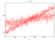
Figure 1: Simulates curves for the two situations

The first situation consists in a two-class problem. The simulated dataset consists of $n=20$ curves, each curve consists of $m=50$ observationas generated as a linear function corrupted by a Gaussian noise as follows. For the $i$th curve ($i=1,\ldots,n$), the $j$th observation ($j=1,\ldots,m$) is generated as follows:

• $y_{ij}=0.3\,x_{ij}+0.4+\sigma_{1}\,\epsilon_{ij}$;

• $y_{ij}=0.1\,x_{ij}+0.5+\sigma_{2}\,\epsilon_{ij}$.

respectively for class 1 and class 2, where $x$ are linearly equally spaced points in the range $[0,1]$, with $\sigma_{1}=0.02$ and $\sigma_{2}=0.03$ are the corresponding noise standard deviations, and $\epsilon_{ij}\sim\mathcal{N}(0,1)$ are standard zero-mean unit variance Gaussian variables. The two classes have the same proportion. Figure 1 (top) shows this dataset where the true value of the number of clusters is $K=2$.

The second situation represents a three-class problem. The simulated dataset consists of $n=100$ arbitrary non-linear curves, each curve consists of $m=50$ observations generated as follows. For the $i$th curve ($i=1,\ldots,n$), the $j$th observation ($j=1,\ldots,m$) is generated as follows:

• $y_{ij}=0.8+0.5\,\exp(-1.5\,x)\,\sin(1.3\pi\,x)+\sigma_{1}\,\epsilon_{ij}$;

• $y_{ij}=0.5+0.8\,\exp(-x)\,\sin(0.9\pi\,x)+\sigma_{2}\,\epsilon_{ij}$;

• $y_{ij}=1+0.5\,\exp(-x)\,\sin(1.2\pi\,x)+\sigma_{3}\,\epsilon_{ij}$.

with $\sigma_{1}=0.04$, $\sigma_{2}=0.04$ and $\sigma_{3}=0.05$. The classes have respectively proportions $\pi_{1}=0.4,\pi_{2}=0.3,\pi_{3}=0.3$. Figure 2 shows the obtained results for the first set of linear curves obtained with a linear regression mixture.

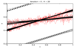
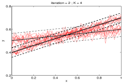
Figure 2: The clustering results obtained with the proposed robust EM-MixReg algorithm for the first set of curves shown in Fig. 1.

For the first dataset, after only two iterations, the majority of illegitimate clusters are discarded and the algorithm converges in 4 iterations and provides the correct clustering results with the actual number of clusters. Figure 3 shows the obtained resulted for the second set of arbitrary non-linear curves obtained with a polynomial regression mixture ($p=3$). The figures show that the algorithm started with a number of clusters equal to the number of curves.

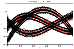
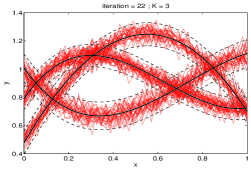
Figure 3: The clustering results obtained with the proposed robust EM-MixReg algorithm for the second set of curves shown in Fig. 1.

It can be seen that for the second data set of non-linear curves, the proposed algorithm also provides accurate results. After starting with a number of clusters $K=100$, the number of clusters decreases rapidly form 100 to 27 after only four iterations. Then the algorithm converges after 22 iterations and provides the actual number of clusters with precise clustering results.

VI Conclusion

In this paper, we presented a new EM algorithm for model-based curve clustering. It optimizes a penalized observed-data log-likelihood using the entropy of the hidden structure. The proposed algorithm overcome both the problem of sensitivity to initialization and determining the optimal number of clusters for standard EM for regression mixtures. The experimental results on simulated data demonstrates the potential benefit of the proposed approach for curve clustering. Future work will concern additional experiments on real data including temporal curves.

References

- [1] J. D. Banfield and A. E. Raftery, “Model-based gaussian and non-gaussian clustering,” Biometrics, vol. 49, no. 3, pp. 803–821, 1993.
- [2] J. C. Bezdek, “Numerical taxonomy with fuzzy sets,” Journal of Mathematical Biology, vol. A, pp. 57–71, 1974.
- [3] C. Biernacki, G. Celeux, and G. Govaert, “Choosing starting values for the EM algorithm for getting the highest likelihood in multivariate gaussian mixture models,” Computational Statistics and Data Analysis, vol. 41, pp. 561–575, 2003.
- [4] C. M. Bishop and C. K. I. Williams, “Gtm: The generative topographic mapping,” Neural Computation, vol. 10, pp. 215–234, 1998.
- [5] G. Celeux and J. Diebolt, “The SEM algorithm a probabilistic teacher algorithm derived from the EM algorithm for the mixture problem,” Computational Statistics Quarterly, vol. 2, no. 1, pp. 73–82, 1985.
- [6] G. Celeux and G. Govaert, “A classification em algorithm for clustering and two stochastic versions,” Computational Statistics and Data Analysis, vol. 14, pp. 315–332, 1992.
- [7] F. Chamroukhi, “Hidden process regression for curve modeling, classification and tracking,” Ph.D. Thesis, Université de Technologie de Compiègne, Compiègne, France, 2010.
- [8] F. Chamroukhi, A. Samé, G. Govaert, and P. Aknin, “Time series modeling by a regression approach based on a latent process,” Neural Networks, vol. 22, no. 5-6, pp. 593–602, 2009.
- [9] ——, “A hidden process regression model for functional data description. application to curve discrimination,” Neurocomputing, vol. 73, no. 7-9, pp. 1210–1221, March 2010.
- [10] J. Cuesta, J. Albertos, and C. Matran, “Trimmed k-means: an attempt to robustify quantizers,” AnnalsofStatistics, vol. 25, pp. 553–576, 1997.
- [11] A. P. Dempster, N. M. Laird, and D. B. Rubin, “Maximum likelihood from incomplete data via the EM algorithm,” Journal of The Royal Statistical Society, B, vol. 39(1), pp. 1–38, 1977.
- [12] M. A. T. Figueiredo and A. K. Jain, “Unsupervised learning of finite mixture models,” IEEE Transactions Pattern Analysis and Machine Intelligence, vol. 24, pp. 381–396, 2000.
- [13] C. Fraley and A. E. Raftery, “Model-based clustering, discriminant analysis, and density estimation,” Journal of the American Statistical Association, vol. 97, pp. 611–631, 2002.
- [14] S. J. Gaffney, “Probabilistic curve-aligned clustering and prediction with regression mixture models,” Ph.D. dissertation, Department of Computer Science, University of California, Irvine, 2004.
- [15] L. Garcia-Escudero and A. Gordaliza, “Robustness properties of -means and trimmed -means,” Journal of the American Statistical Association, vol. 94, pp. 956–969, 1999.
- [16] J. A. Hartigan and M. A. Wong, “A K-means clustering algorithm,” Applied Statistics, vol. 28, pp. 100–108, 1979.
- [17] T. Hastie, R. Tibshirani, and J. Friedman, The Elements of Statistical Learning, Second Edition: Data Mining, Inference, and Prediction, second edition ed., ser. Springer Series in Statistics. Springer, 2010.
- [18] R. A. Jacobs, M. I. Jordan, S. J. Nowlan, and G. E. Hinton, “Adaptive mixtures of local experts,” Neural Computation, vol. 3, no. 1, pp. 79–87, 1991.
- [19] G. M. James and C. Sugar, “Clustering for sparsely sampled functional data,” Journal of the American Statistical Association, vol. 98, no. 462, 2003.
- [20] T. Kohonen, Self-Organizing Maps, third edition ed., ser. Information Sciences. Springer, 2001.
- [21] S. Kong and B. Kosko, “Differential competitive learning for centroid estimation and phoneme recognition,” IEEE Transactions on Neural Networks, vol. 2, no. 1, pp. 118–124, 1991.
- [22] J. B. MacQueen, “Some methods for classification and analysis of multivariate observations,” in Proceedings of the 5th Berkeley Symposium on Mathematical Statistics and Probability, 1967, pp. 281–297.
- [23] G. J. McLachlan and T. Krishnan, The EM algorithm and extensions. Wiley, 1997.
- [24] G. J. McLachlan and D. Peel., Finite mixture models. Wiley, 2000.
- [25] G. McLachlan and K. Basford, Mixture Models: Inference and Applications to Clustering. Marcel Dekker, New York, 1988.
- [26] J. O. Ramsay and B. W. Silverman, Functional Data Analysis, ser. Springer Series in Statistics. Springer, June 2005.
- [27] C. K. Reddy, H.-D. Chiang, and B. Rajaratnam, “Trust-tech-based expectation maximization for learning finite mixture models,” IEEE Transactions Pattern Analysis and Machine Intelligence, vol. 30, no. 7, pp. 1146–1157, 2008.
- [28] S. Richardson and P. J. Green, “On Bayesian Analysis of Mixtures with an Unknown Number of Components (with discussion),” Journal of the Royal Statistical Society: Series B (Methodological), vol. 59, no. 4, pp. 731–792, 1997.
- [29] A. Samé, F. Chamroukhi, G. Govaert, and P. Aknin, “Model-based clustering and segmentation of time series with changes in regime,” Adv. in Data Analysis and Classification, vol. 5, no. 4, pp. 1–21, 2011.
- [30] G. Schwarz, “Estimating the dimension of a model,” Annals of Statistics, vol. 6, pp. 461–464, 1978.
- [31] M.-S. Yang, C.-Y. Lai, and C.-Y. Lin, “A robust em clustering algorithm for gaussian mixture models,” Pattern Recognition, vol. 45, no. 11, pp. 3950–3961, Nov. 2012.