Model-based clustering with Hidden Markov Model regression for time series with regime changes

Abstract

This paper introduces a novel model-based clustering approach for clustering time series which present changes in regime. It consists of a mixture of polynomial regressions governed by hidden Markov chains. The underlying hidden process for each cluster activates successively several polynomial regimes during time. The parameter estimation is performed by the maximum likelihood method through a dedicated Expectation-Maximization (EM) algorithm. The proposed approach is evaluated using simulated time series and real-world time series issued from a railway diagnosis application. Comparisons with existing approaches for time series clustering, including the stand EM for Gaussian mixtures, $K$-means clustering, the standard mixture of regression models and mixture of Hidden Markov Models, demonstrate the effectiveness of the proposed approach.

I Introduction

The work presented in this paper relates to the diagnosis of the railway switches which enable trains to be guided from one track to another at a railway junction. The switch is controlled by an electrical motor and the considered time series are the time series of the consumed power during the switch operations. These time series present changes in regime due to successive mechanical motions involved in a switch operation (see Figure 4). The kind of time series studied here may also be referred to as longitudinal data, functional data, curves or signals. The diagnosis task can be achieved through the analysis of these time series issued from the switch operations to identify possible faults. However, the large amount of data makes the manual labeling task onerous for the experts. Therefore, the main concern of this work is to propose a data preprocessing approach that allows for automatically identifying homogeneous groups in a set of time series. Thus, the founded groups can then be easily treated and interpreted by the maintenance staff in order to identify faults. This preliminary task can be achieved through an unsupervised classification (clustering) approach. In this paper, we focus on model-based clustering approaches for their well established statistical properties and the suitability of the Expectation-Maximization algorithm [1] to this unsupervised framework.

In this context, since the time series present regime changes, basic polynomial regression models are not suitable. An alternative approach may consist in using cubic splines to approximate each set of time series [2] but this requires the setting of knots which may a combinatory complex task. Generative models have been developed by Gaffney & Smyth [3, 4] which consist in clustering time series with mixture of regressions or random effect models. Liu & Yang [5] proposed a clustering approach based on random effect spline regression where the time series are represented by B-spline basis functions. However, the first approach does not address the problem of changes in regimes and the second one requires the setting of the spline knots. Another approach based on splines is concerned with clustering sparsely sampled time series [2]. We note that all these approaches use the EM algorithm to estimate the model parameters. Another clustering approach consist in the evolutionary clustering approach [6], however, in this paper, the structure of the model is fixed over time.

In this paper, a specific generative mixture model is proposed to cluster time series presenting regime changes. In this mixture model, each component density is the one of a specific regression model that incorporates a hidden Markov chain allowing for transitions between different polynomial regression models over time. The proposed model can be seen as an extension of the model-clustering approach using mixture of standard HMMs introduced by Smyth [7], by considering a polynomial regression Hidden Markov Model rather than a standard HMM. In addition, owing to the fact that the real time series of switch operations we aim to model consist of successive phases, order constraints are imposed on the hidden states.

This paper is organized as follows. Section 2 provides an account of the model-based clustering approaches using mixture of regression models and mixture of Hidden Markov Models. Section 3 introduces the proposed model-based time series clustering and its parameter estimation via a dedicated EM algorithm. Finally, section 4 deals with the experimental study carried out on simulated time series and real-world time series of the switch operations to asses the proposed approach by comparing it to existing time series clustering approaches, in particular, the mixture of regression approach [3, 8] and the standard mixture of HMMs [7].

II Model-based clustering for time series

II-A Model-based clustering

Model-based clustering [9, 10, 11], generally used for multidimensional data, is based on the finite mixture model formulation [12]. In the finite mixture approach for cluster analysis, the data probability density function is assumed to be a mixture of $K$ components densities, each component density being associated with a cluster. The problem of clustering therefore becomes the one of estimating the parameters of the assumed mixture model (e.g, estimating the mean vectors and the covariance matrices in the case of Gaussian mixtures). The parameters of the mixture density are generally estimated by maximizing the observed-data likelihood via the well-known Expectation-Maximization (EM) algorithm [1, 13]. After performing the probability density estimation, the obtained posterior cluster probabilities are then used to determine the cluster memberships through the maximum a posteriori (MAP) principle and therefore to provide a partition of the data into $K$ clusters.

Model-based clustering approaches have also been introduced to generalize the standard multivariate mixture model for the analysis of time series data, which are also referred to as longitudinal data, functional data or sequences. In that case, the individuals are presented as functions or curves rather than a vector of a reduced dimension. In that context, one can distinguish the regression mixture approaches [3, 8], including polynomial regression and spline regression. Random effects approaches that are based on polynomial regression [4] or spline regression [5]. Another approach based on splines is concerned with clustering sparsely sampled time series [2]. All these approaches use the EM algorithm to estimate the model parameters. In the following section we will give an overview of these model-based clustering approaches for time series.

Let $\mathbf{Y}=(\mathbf{y}_{1},\ldots,\mathbf{y}_{n})$ be a set of $n$ independent time series and let $(h_{1},\ldots,h_{n})$ be the associated unknown cluster labels with $h_{i}\in\{1,\ldots,K\}$. We assume that each time series $\mathbf{y}_{i}$ consists of $m$ measurements (or observations) $\mathbf{y}_{i}=(y_{i1},\ldots,y_{im})$, regularly observed at the time points $\mathbf{t}=(t_{1},\ldots,t_{m})$ with $t_{1}<\ldots<t_{m}$.

II-B Related work on model-based clustering for time series

II-B1 Mixture of regression models

In this section we describe time series clustering approaches based on polynomial regression mixtures and polynomial spline regression mixtures [3, 8]. The regression mixture approaches assume that each times series is drawn from one of $K$ clusters of time series which are mixed at random in proportion to the relative cluster sizes $(\alpha_{1},\ldots,\alpha_{K})$. Each cluster of time series is modeled by either a polynomial regression model or a spline regression model. Thus, the conditional mixture density of a time series $\mathbf{y}_{i}$ can be written as:

$$f(\mathbf{y}_{i}|\mathbf{t};\boldsymbol{\Psi}) = \sum_{k=1}^{K}\alpha_{k}\ \mathcal{N}(\mathbf{y}_{i};\mathbf{X}\boldsymbol{\beta}_{k},\sigma_{k}^{2}\textbf{I}_{m}),$$ (1)

where the $\alpha_{k}$’s defined by $\alpha_{k}=p(h_{i}=k)$ are the non-negative mixing proportions that sum to 1, $\boldsymbol{\beta}_{k}$ is the $(p+1)$-dimensional coefficient vector of the $k$th polynomial regression model, $p$ being the polynomial degree, and $\sigma_{k}^{2}$ is the associated noise variance. The matrix $\mathbf{X}$ is the $m\times(p+1)$ design matrix with rows $\mathbf{t}_{j}=(1,t_{j},t_{j}^{2},\ldots,t_{j}^{p})$ for $j=1,\ldots,m$ and $\textbf{I}_{m}$ is the identity matrix of dimension $m$. The model is therefore described by the parameter vector $\boldsymbol{\Psi}=(\alpha_{1},\ldots,\alpha_{k},\boldsymbol{\Psi}_{1},\ldots,\boldsymbol{\Psi}_{K})$ with $\boldsymbol{\Psi}_{k}=(\boldsymbol{\beta}_{k},\sigma_{k}^{2})$.

Parameter estimation is performed by maximizing the observed-data log-likelihood of $\boldsymbol{\Psi}$:

$$\mathcal{L}(\boldsymbol{\Psi}) = \sum_{i=1}^{n}\log\sum_{k=1}^{K}\alpha_{k}\ \mathcal{N}(\mathbf{y}_{i};\mathbf{X}\boldsymbol{\beta}_{k},\sigma_{k}^{2}\textbf{I}_{m}).$$ (2)

This log-likelihood, which can not be maximized in a closed form, is maximized by the EM algorithm [1]. The details of the EM algorithm for the mixture of regressions models and the corresponding updating formula can be found in [3, 8].

Once the model parameters are estimated, a partition of the data is then computed by maximizing the posterior cluster probabilities defined by:

$$\!\!\!\!\!\!\tau_{ik} = p(h_{i}=k|\mathbf{y}_{i},\mathbf{t};\boldsymbol{\Psi})\!\!=\!\!\frac{\alpha_{k}\mathcal{N}\big{(}\mathbf{y}_{i};\mathbf{X}\boldsymbol{\beta}^{T}_{k},\sigma^{2}_{k}\textbf{I}_{m}\big{)}}{\sum_{k^{\prime}=1}^{R}\alpha_{k^{\prime}}\mathcal{N}(\mathbf{y}_{i};\mathbf{X}\boldsymbol{\beta}^{T}_{k^{\prime}},\sigma^{2}_{k^{\prime}}\textbf{I}_{m})}\cdot$$ (3)

The mixture of regression models however do not address the problem of regime changes within times series. Indeed, they assume that each cluster present a stationary behavior described by a single polynomial mean function. The spline regression mixture does not address automatically the regime changes as the knots are generally fixed in advance and the optimization of their location needs a strong computational load. These approach may therefore have limitations in the case of time series presenting changes in regime. To overcome these limitations, one way is to proceed as in the case of sequential data modeling in which it is assumed that the observed sequence (in this case a times series) is governed by a hidden process which enables for switching from one state to another among $R$ states. The used process in general is an $R$ state Markov chain for each time series. This leads to the mixture of Hidden Markov Models [7] which we describe in the following section.

II-B2 Mixture of HMMs for clustering sequences

In this section we describe the mixture of Hidden Markov Models (HMMs) initiated by Smyth [7] and used for clustering sequences, which can therefore be applied to time series. Since the model in this case includes an HMM formulation, let us first recall the principle of HMMs.

Hidden Markov Models (HMMs)

Hidden Markov Models (HMMs) are a class of latent data models appropriate for sequential data. They are widely used in many application domains, including speech recognition, image analysis, time series prediction [14, 15], etc. In an HMM, the observation sequence (or a time series) $\mathbf{y}_{i}=(y_{i1},\ldots,y_{im})$ is assumed to be governed by a hidden state sequence $\mathbf{z}_{i}=(z_{i1},\ldots,z_{im})$ where the discrete random variable $z_{ij}\in\{1,\ldots,R\}$ represents the unobserved state associated with $y_{ij}$ at instant $t_{j}$. The state sequence $\mathbf{z}_{i}$ is generally assumed to be a first order homogeneous Markov chain, that is, the current state given the previous state sequence depends only on the previous state. Formally we have :

$$p(z_{i1}|z_{i,j-1},z_{i,j-2},\ldots,z_{i1})=p(z_{ij}|z_{i,j-1})\ \forall j>1.$$ (4)

The transition probabilities $p(z_{ij}|z_{i,j-1})$ do not depend on $t$ in the case of an homogeneous Markov chain. An HMM is therefore fully determined by the initial state distribution $\boldsymbol{\pi}=(\pi_{1},\ldots,\pi_{R})$ where $\pi_{r}=p(z_{1}=r)$ satisfying $\sum_{r}\pi_{r}=1$, the matrix of transition probabilities $\boldsymbol{A}$ with elements $A_{\ell r}=p(z_{ij}=r|z_{i,j-1}=\ell)$ satisfying $\sum_{r}A_{\ell r}=1$ and the parameters $(\boldsymbol{\Psi}_{1},\ldots,\boldsymbol{\Psi}_{R})$ of the emission probabilities $p(y_{ij}|z_{ij}=r;\boldsymbol{\Psi}_{r})$. The distribution of a particular configuration of the latent state sequence $\mathbf{z}_{i}=(z_{i1},\ldots,z_{im})$ is is given by:

$$p(\mathbf{z}_{i};\boldsymbol{\pi},\boldsymbol{A})=p(z_{i1};\boldsymbol{\pi})\prod_{j=2}^{m}p(z_{ij}|z_{i,j-1};\boldsymbol{A}),$$ (5)

and from the conditional independence property of the HMM, that is the observation sequence is independent given a particular configuration of the hidden state sequence, the conditional distribution of the observed sequence is therefore given by:

$$p(\mathbf{y}_{i}|\mathbf{z}_{i};\boldsymbol{\Psi})=\prod_{j=1}^{m}p(y_{ij}|z_{ij};\boldsymbol{\Psi}).$$ (6)

From (5) and (6), we can then get the following joint distribution $p(\mathbf{y}_{i},\mathbf{z}_{i};\boldsymbol{\Psi})=p(\mathbf{z}_{i};\boldsymbol{\pi},\boldsymbol{A})p(\mathbf{y}_{i}|\mathbf{z}_{i};\boldsymbol{\Psi}).$

Mixture of Hidden Markov Models

The mixture of HMMs integrates the HMM into a mixture framework to perform sequence clustering [7, 16]. In this probabilistic model-based clustering, an observation sequence (in this case a time series) is assumed to be generated according to a mixture of $K$ components, each component being an HMM. Formally, each time series $\mathbf{y}_{i}$ is distributed according to the following mixture distribution:

$$f(\mathbf{y}_{i};\boldsymbol{\Psi})=\sum_{k=1}^{K}\alpha_{k}f_{k}(\mathbf{y}_{i};\boldsymbol{\Psi}_{k}),$$ (7)

where the component density $f_{k}(\mathbf{y}_{i};\boldsymbol{\Psi}_{k})=p(\mathbf{y}_{i}|h_{i}=k;\boldsymbol{\Psi}_{k})$ is assumed to be a $K$ state HMM, typically with univariate Gaussian emission probabilities in this case of univariate time series. The HMM associated with the $k$th cluster is determined by the parameters $\boldsymbol{\Psi}_{k}=(\boldsymbol{\pi}_{k},\boldsymbol{A}_{k},\mu_{k1},\ldots,\mu_{kR},\sigma^{2}_{k1},\ldots,\sigma^{2}_{kR})$ where $\boldsymbol{\pi}_{k}$ is the initial state distribution for the HMM associated with cluster $k$, $\boldsymbol{A}_{k}$ is the corresponding transition matrix and $(\mu_{kr},\sigma^{2}_{kr})$ are respectively the constant mean and the variance of an univariate Gaussian density associated with the $r$th state in cluster $k$. By using the joint distribution of $\mathbf{y}$ and $\mathbf{z}$ which can be deduced from (5) and (6), the distribution of a time series issued from the $k$th cluster is therefore given by:

$$f_{k}(\mathbf{y}_{i};\boldsymbol{\Psi}_{k}) = \sum_{\mathbf{z}_{i}}p(z_{i1};\boldsymbol{\pi}_{k})\prod_{j=2}^{m}p(z_{ij}|z_{i,j-1};\boldsymbol{A}_{k})\times$$ (8)

$$\prod_{j=1}^{m}\mathcal{N}(y_{ij};\mu_{kz_{ij}},\sigma_{kz_{ij}}^{2}).$$

Two different approaches can be adopted for estimating this mixture of HMMs. Two such techniques are the hard-clustering $K$-means-like approach and the soft-clustering EM approach. The $K$-means-like approach for hard clustering have been used in [7] in which the optimized function is the complete-data log-likelihood. The resulting clustering scheme consists of assigning sequences to clusters at each iteration and using only the sequences assigned to a cluster for re-estimation of its HMM parameters. The soft clustering approach is described in [16] where the model parameters are estimated in a maximum likelihood framework by the EM algorithm.

In this standard mixture of HMMs, each state is represented by its scalar mean in the case of univariate time series. However, in many applications, in particular in signal processing or time series analysis, as in the case of the time series issued from the switch operations, it is often useful to represent a state by a polynomial rather than a scalar (constant function of time). This assumption should be more suitable for fitting the non-linear regimes governing the time series. In addition, when the regimes are ordered in time, the hidden process governing the time series can be adapted by imposing order constraints on the states of the Markov chain. These generalizations are integrated in the proposed mixture of HMM regression models which we present in the following section.

III The proposed mixture of HMM regression models for time series clustering

III-A Model definition

The proposed model assumes that each time series $\mathbf{y}_{i}$ is issued from one of $K$ clusters where, within each cluster $k$ $(k=1,\ldots,K)$, each time series is generated by $R$ unobserved polynomial regimes. The transition from one regime to another is governed by an homogeneous Markov Chain of first order. Formally, the distribution of a times series $\mathbf{y}_{i}$ is defined by the following conditional mixture density:

$$f(\mathbf{y}_{i}|\mathbf{t};\boldsymbol{\Psi})=\sum_{k=1}^{K}\alpha_{k}f_{k}(\mathbf{y}_{i}|\mathbf{t};\boldsymbol{\Psi}_{k}),$$ (9)

where each component density $f_{k}(.)$ associated with the $k$th cluster is a polynomial HMM regression model (see [17] for details on HMM regression for a single time series). In this clustering context with HMM regression, given the cluster $h_{i}=k$, the time series $\mathbf{y}_{i}=(y_{i1},\ldots,y_{im})$ is assumed to be generated by the following regression model :

$$y_{ij}=\boldsymbol{\beta}^{T}_{kz_{ij}}\mathbf{t}_{j}+\sigma_{kz_{ij}}\epsilon_{ij}\quad(j=1,\ldots,m)$$ (10)

where $\boldsymbol{\beta}_{kr}$ is the $(p+1)$-dimensional coefficients vector of the $r$th polynomial regression model of cluster $k$, $\sigma_{kr}^{2}$ is its associated noise variance and the $\epsilon_{ij}$ are independent random variables distributed according to a Gaussian distribution with zero mean and unit variance. The hidden state sequence $\mathbf{z}_{i}=(z_{i1},\ldots,z_{im})$ is assumed to be Markov chain of parameters $(\boldsymbol{\pi}_{k},\mathbf{A}_{k})$. The proposed model is illustrated by the graphical representation in Figure 1.

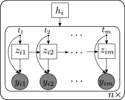
Figure 1: Graphical model structure for the proposed mixture of HMM regression models (MixHMMR).

Each component density is therefore parametrized by the parameter vector $\boldsymbol{\Psi}_{k}=(\boldsymbol{\pi}_{k},\boldsymbol{A}_{k},\boldsymbol{\beta}_{k1},\ldots,\boldsymbol{\beta}_{kR},\sigma_{k1}^{2},\ldots,\sigma_{kR}^{2})$ and is given in a similar way as for (8) by:

$$f_{k}(\mathbf{y}_{i}|\mathbf{t};\boldsymbol{\Psi}_{k}) = \sum_{\mathbf{z}_{i}}p(z_{i1};\boldsymbol{\pi}_{k})\prod_{j=2}^{m}p(z_{ij}|z_{i,j-1};\boldsymbol{A}_{k})\times$$ (11)

$$\prod_{j=1}^{m}\mathcal{N}(y_{ij};\boldsymbol{\beta}^{T}_{kz_{ij}}\mathbf{t}_{j},\sigma_{kz_{ij}}^{2}).$$

III-B A HMMR with order constraints

Since the time series we aim to model here consist of successive contiguous regimes, we impose order constraints on the hidden states by imposing the following constraints on the transition probabilities for each cluster $k$. These constraints imply that no transitions are allowed for the phases whose indexes are lower than the current phase and no jumps of more than one state are possible. Formally, we have:

$$A_{k\ell r}=p(z_{ijk}=r|z_{i(j-1)k}=\ell,h_{i}=k)=0\ \mbox{if}\ r<\ell$$

and

$$A_{k\ell r}=p(z_{ijk}=r|z_{i(j-1)k}=\ell,h_{i}=k)=0\ \mbox{if}\ r>\ell+1.$$

This constrained model is a particular case of the well known left-right model [14].

III-C Remark: Link with the polynomial regression mixture

The particular case for which the proposed model is defined with a single regime $R=1$ for each cluster $k$, corresponds to the polynomial regression mixture model.

The next section presents the parameter estimation by the maximum likelihood method.

III-D Parameter estimation

The proposed MixHMMR model is described by the parameter vector $\boldsymbol{\Psi}=(\alpha_{1},\ldots,\alpha_{K},\boldsymbol{\Psi}_{1},\ldots,\boldsymbol{\Psi}_{K}).$ Parameter estimation is performed by maximizing the observed-data log-likelihood of $\boldsymbol{\Psi}$ :

$$\mathcal{L}(\boldsymbol{\Psi}) = \log p(\mathbf{y}_{1},\ldots,\mathbf{y}_{n}|\mathbf{t};\boldsymbol{\Psi})=\log\prod_{i=1}^{n}p(\mathbf{y}_{i}|\mathbf{t};\boldsymbol{\Psi})$$ (12)

$$= \sum_{i=1}^{n}\log\sum_{k=1}^{K}\alpha_{k}\sum_{\mathbf{z}_{i}}p(z_{i1};\boldsymbol{\pi}_{k})\prod_{j=2}^{m}p(z_{ij}|z_{i,j-1};\boldsymbol{A}_{k})\times$$

$$\prod_{j=1}^{m}\mathcal{N}(y_{ij};\boldsymbol{\beta}^{T}_{kz_{ij}}\mathbf{t}_{j},\sigma_{kz_{ij}}^{2}).$$

The maximization of this log-likelihood cannot be performed in a closed form. We maximize it iteratively by using a dedicated EM algorithm. With this specification of the EM algorithm, the complete-data for the proposed model consist of the observed set of curves $\mathbf{Y}=(\mathbf{y}_{1},\ldots,\mathbf{y}_{n})$, their corresponding cluster labels $\mathbf{h}=(h_{1},\ldots,h_{n})$ and the matrix of regime (state) labels $\mathbf{Z}=(\mathbf{z}_{1},\ldots,\mathbf{z}_{n})$, $\mathbf{z}_{i}$ being the hidden state sequence associated with $\mathbf{y}_{i}$. The complete-data likelihood of $\boldsymbol{\Psi}$ is therefore given by:

$$p(\mathbf{Y},\mathbf{h},\mathbf{Z}|\mathbf{t};\boldsymbol{\Psi}) = p(\mathbf{h})p(\mathbf{Y},\mathbf{Z}|\mathbf{h},\mathbf{t};\boldsymbol{\Psi})$$

$$= p(\mathbf{h})p(\mathbf{Z}|\mathbf{h},\mathbf{t};\boldsymbol{\Psi})p(\mathbf{Y}|\mathbf{h},\mathbf{Z},\mathbf{t};\boldsymbol{\Psi})$$

$$= \prod_{i=1}^{n}p(h_{i})p(\mathbf{z}_{i}|\mathbf{t};\boldsymbol{\pi}_{h_{i}},\boldsymbol{A}_{h_{i}})p(\mathbf{y}_{i}|\mathbf{z}_{i},\mathbf{t};\boldsymbol{\theta}_{h_{i}}).$$

Then, by using some elementary calculation details, we get the complete complete-data log-likelihood:

$$\!\!\!\!\!\!\!\!\!\mathcal{L}_{c}(\boldsymbol{\Psi}) = \log p(\mathbf{Y},\mathbf{h},\mathbf{Z}|\mathbf{t};\boldsymbol{\Psi})$$ (13)

$$= \sum_{k=1}^{K}\Big{[}\sum_{i=1}^{n}h_{ik}\log\alpha_{k}+\sum_{i=1}^{n}\sum_{r=1}^{R}h_{ik}z_{i1kr}\log\pi_{kr}$$

$$+\sum_{i=1}^{n}\sum_{j=2}^{m}\sum_{r,\ell=1}^{R}h_{ir}z_{ijkr}z_{i(j-1)k\ell}\log A_{k\ell r}$$

$$+\sum_{i=1}^{n}\sum_{j=1}^{m}\sum_{r=1}^{R}h_{ik}z_{ijkr}\log\mathcal{N}(y_{ij};\boldsymbol{\beta}^{T}_{kr}\mathbf{t}_{j},\sigma^{2}_{kr})\Big{]}$$

where we have used the following indicator binary variables for indicating the cluster memberships and the regime meberships for a given cluster, that is:

• $h_{ik}=1$ if $h_{i}=k$ (i.e., $\mathbf{y}_{i}$ belongs to cluster $k$) and $h_{ik}=0$ otherwise.

• $z_{ijkr}=1$ if $z_{ijk}=r$ (i.e., the $i$th times series $\mathbf{y}_{i}$ belongs to cluster $k$ and its $m$th observation $y_{ij}$ belongs to regime $r$) and $z_{ijkr}=0$ otherwise.

The next section gives the proposed EM algorithm for the mixture of HMM regression models.

III-D1 The dedicated EM algorithm

The EM algorithm for the proposed MixHMMR model starts from an initial parameter $\boldsymbol{\Psi}^{(0)}$ and alternates between the two following steps until convergence:

E Step

Compute the expected complete-data log-likelihood given the time series $\mathbf{Y}$, the time vector $\mathbf{t}$ and the current value of the parameter $\boldsymbol{\Psi}$ denoted by $\boldsymbol{\Psi}^{(q)}$:

$$Q(\boldsymbol{\Psi},\boldsymbol{\Psi}^{(q)}) = \mathbb{E}\big{[}\mathcal{L}_{c}(\boldsymbol{\Psi})|\mathbf{Y},\mathbf{t};\boldsymbol{\Psi}^{(q)}\big{]}$$ (14)

It can be easily shown that this conditional expectation is given by:

$$Q(\boldsymbol{\Psi},\boldsymbol{\Psi}^{(q)})=Q_{1}(\alpha_{k})+\sum_{k=1}^{K}\Big{[}Q_{2}(\boldsymbol{\pi}_{k},\mathbf{A}_{k})+Q_{3}(\boldsymbol{\beta}_{kr},\sigma^{2}_{kr})\Big{]},\\$$

where

$$Q_{1}(\alpha_{k})=\sum_{k=1}^{K}\sum_{i=1}^{n}\tau_{ik}^{(q)}\log\alpha_{k},$$

$$Q_{2}(\boldsymbol{\pi}_{k},\boldsymbol{A}_{k})=\sum_{r=1}^{R}\sum_{i=1}^{n}\tau_{ik}^{(q)}\big{[}\gamma^{(q)}_{ik1}\log\pi_{kr}+\sum_{j=2}^{m}\sum_{\ell=1}^{R}\xi^{(q)}_{ijk\ell r}\log A_{k\ell r}\big{]},$$

$$Q_{3}(\boldsymbol{\beta}_{kr},\sigma^{2}_{kr})=\sum_{r=1}^{R}\sum_{i=1}^{n}\sum_{j=1}^{m}\tau_{ik}^{(q)}\gamma^{(q)}_{ijkr}\log\mathcal{N}(y_{ij};\boldsymbol{\beta}^{T}_{kr}\mathbf{t}_{j},\sigma^{2}_{kr})$$

where

• $\tau^{(q)}_{ik}=p(h_{i}=k|\mathbf{y}_{i},\mathbf{t};\boldsymbol{\Psi}^{(q)})$ is the posterior probability of cluster $k$;

• $\gamma^{(q)}_{ijkr}=p(z_{ijk}=r|\mathbf{y}_{i},\mathbf{t};\boldsymbol{\Psi}_{k}^{(q)})$ is the posterior probability of the $k$th polynomial regime for the $k$th cluster,

• $\xi^{(q)}_{ijkr\ell}=p(z_{ijk}=r,z_{i(j-1)k}=\ell|\mathbf{y}_{i},\mathbf{t};\boldsymbol{\Psi}_{k}^{(q)})$ is the joint probability of having the regime $r$ at time $t_{j}$ and the regime $\ell$ at time $t_{j-1}$ in cluster $k$.

As shown in the expression of $Q$, this step requires only the computation of the probabilities $\tau^{(q)}_{ik}$, $\gamma^{(q)}_{ijkr}$ and $\xi^{(q)}_{ijk\ell r}$. The probabilities $\gamma^{(q)}_{ijkr}$ and $\xi^{(q)}_{ijk\ell r}$ for each time series $\mathbf{y}_{i}$ $(i=1,\ldots,n)$ are computed as follows [14]:

$$\gamma^{(q)}_{ijkr}=\frac{a^{(q)}_{ijkr}b^{(q)}_{ijkr}}{\sum_{\ell=1}^{R}a^{(q)}_{ijk\ell}b^{(q)}_{ijk\ell}}$$ (15)

and

$$\xi^{(q)}_{ijk\ell r}=\frac{a^{(q)}_{i(j-1)\ell}\ A^{(q)}_{k\ell r}\mathcal{N}(y_{ij};\boldsymbol{\beta}^{(q)T}_{kr}\mathbf{t}_{j},\sigma_{kr}^{(q)2})b^{(q)}_{ijkr}}{\sum_{r,\ell=1}^{R}a^{(q)}_{i(j-1)\ell k}\ A^{(q)}_{k\ell r}\mathcal{N}(y_{ij};\boldsymbol{\beta}^{(q)T}_{kr}\mathbf{t}_{j},\sigma_{kr}^{(q)2})\ b^{(q)}_{ijkr}}.$$ (16)

where the quantities $a_{ijkr}$ and $b_{ijkr}$ are respectively the forward probabilities and the backward probabilities, which are in this context given by:

$$a_{ijkr}=p(y_{i1},\ldots,y_{ij},z_{ijk}=r|\mathbf{t};\boldsymbol{\Psi}_{k}),$$ (17)

and

$$b_{ijkr}=p(y_{i,j+1},\ldots,y_{im}|z_{ijk}=r,|\mathbf{t};\boldsymbol{\Psi}_{k})$$ (18)

and are recursively computed via the well-known forward-backward (Baum-Welch) procedure [18, 14].

The posterior cluster probabilities $\tau_{ik}^{(q)}$ that the time series $\mathbf{y}_{i}$ belongs to cluster $k$ are computed as follows:

$$\tau^{(q)}_{ik}=\frac{\alpha_{k}^{(q)}f_{k}(\mathbf{y}_{i}|\mathbf{t};\boldsymbol{\Psi}^{(q)}_{k})}{\sum_{k^{\prime}=1}^{K}\alpha_{k^{\prime}}^{(q)}f_{k^{\prime}}(\mathbf{y}_{i}|\mathbf{t};\boldsymbol{\Psi}^{(q)}_{k^{\prime}})},$$ (19)

where the conditional probability distribution of the time series $\mathbf{y}_{i}$ given a cluster $k$, which can be expressed in function of the forward variables $a_{ijkr}$ (17) as:

$$f_{k}(\mathbf{y}_{i}|\mathbf{t};\boldsymbol{\Psi}^{(q)}_{k})=p(y_{i1},\ldots,y_{im}|\mathbf{t};\boldsymbol{\Psi}^{(q)}_{k})=\sum_{r=1}^{R}a_{imkr},$$

is therefore obtained after the forward procedure.

M-step

In this step, the value of the parameter $\boldsymbol{\Psi}$ is updated by maximizing the expected complete-data log-likelihood with respect to $\boldsymbol{\Psi}$, that is:

$$\boldsymbol{\Psi}^{(q+1)}=\arg\max_{\boldsymbol{\Psi}}Q(\boldsymbol{\Psi},\boldsymbol{\Psi}^{(q)}).$$ (20)

The maximization of $Q$ can be performed by separately maximizing the functions $Q_{1}$, $Q_{2}$ and $Q_{3}$. The maximization of $Q_{1}$ w.r.t the mixing proportions $\alpha_{k}$ is the one of a standard mixture model. The updates are given by:

$${\alpha_{k}}^{(q+1)}=\frac{\sum_{i=1}^{n}\tau_{ik}^{(q)}}{n}\cdot$$ (21)

The maximization of $Q_{2}$ w.r.t the parameters $(\boldsymbol{\pi}_{k},\mathbf{A}_{k})$ correspond to a weighted version of updating the parameters of the Markov chain in a standard HMM. The weights in this case are the posterior cluster probabilities $\tau_{ik}$ and the updates are given by:

$$\pi_{kr}^{(q+1)}=\frac{\sum_{i=1}^{n}\tau_{ik}^{(q)}\gamma^{(q)}_{i1kr}}{\sum_{i=1}^{n}\tau_{ik}^{(q)}},$$ (22)

and

$$A^{(q+1)}_{k\ell r})=\frac{\sum_{i=1}^{n}\sum_{j=2}^{m}\tau_{ik}^{(q)}\xi^{(q)}_{ijk\ell r}}{\sum_{i=1}^{n}\sum_{j=2}^{m}\tau_{ik}^{(q)}\gamma^{(q)}_{ijkr}}\cdot$$ (23)

Maximizing $Q_{3}$ with respect to regression parameters $\boldsymbol{\beta}_{kr}$ for $k=1,\ldots,K$ and $r=1,\ldots,R$ consists in analytically solving $K\times R$ weighted least-squares problems where the weights consists in both the posterior cluster probabilities $\tau_{ik}$ and the posterior regimes probabilities $\gamma^{(q)}_{ijkr}$ for each cluster $k$. The parameter updates are given by:

$${\boldsymbol{\beta}}_{kr}^{(q+1)}=\Big{[}\mathbf{X}^{T}\big{(}\sum_{i=1}^{n}\tau_{ik}^{(q)}\mathbf{W}_{ikr}^{(q)}\big{)}\mathbf{X}\Big{]}^{-1}\mathbf{X}^{T}\big{(}\sum_{i=1}^{n}\tau_{ik}^{(q)}\mathbf{W}_{ikr}^{(q)}\mathbf{y}_{i}\big{)},$$ (24)

where $\mathbf{W}_{ikr}^{(q)}$ is an $m$ by $m$ diagonal matrix whose diagonal elements are the weights $\{\gamma_{ijkr}^{(q)};j=1,\ldots,m\}$.

Finally, the maximization of $Q_{3}$ with respect to noise variances $\sigma_{kr}^{2(q+1)}$ consists in a weighted variant of the problem of estimating the variance of an univariate Gaussian density. The updating formula is given by:

$$\sigma_{kr}^{2(q+1)}=\frac{\sum_{i=1}^{n}\tau_{ik}^{(q)}|\!|\sqrt{\mathbf{W}_{ikr}^{(q)}}(\mathbf{y}_{i}-\mathbf{X}\boldsymbol{\beta}_{kr}^{(q+1)})|\!|^{2}}{\sum_{i=1}^{n}\tau_{ik}^{(q)}\text{trace}(\mathbf{W}_{irk}^{(q)})},$$ (25)

where $|\!|\cdot|\!|$ is the euclidian norm.

The pseudo code 1 summarizes the EM algorithm for the proposed MixHMMR model.

Algorithm 1 Pseudo code of the proposed algorithm.

Inputs: $(\mathbf{y}_{1},\ldots,\mathbf{y}_{n}),(t_{1},\ldots,t_{m}),K,R,p$

1:  Initialize: $\boldsymbol{\Psi}^{(0)}=(\alpha^{(0)}_{1},\ldots,\alpha^{(0)}_{R},\boldsymbol{\Psi}_{1}^{(0)},\ldots,\boldsymbol{\Psi}_{K}^{(0)})$

2:  fix a threshold $\epsilon>0$

3:  set $q\leftarrow 0$ (EM iteration)

4:  while increment in log-likelihood $>\epsilon$ do

5:     E-Step:

6:     for $k=1,\ldots,K$ do

7:        forward-backward procedure:

8:        for $r=1,\ldots,R$ do

9:           compute $\gamma_{ijkr}^{(q)}$ for $i=1,\ldots,n$ and $j=1,\ldots,m$ using Equation (15)

10:           for $\ell=1,\ldots,R$ do

11:              compute $\xi_{ijk\ell r}^{(q)}$ for $i=1,\ldots,n$ and $j=1,\ldots,m$ using Equation (16)

12:           end for

13:        end for

14:        compute $\tau_{ik}^{(q)}$ for $i=1,\ldots,n$ using Equation (19)

15:     end for

16:     M-Step:

17:     for $k=1,\ldots,K$ do

18:        compute $\alpha_{k}^{(q+1)}$ using Equation (21)

19:        for for $r=1,\ldots,R$ do

20:           compute $\boldsymbol{\pi}_{kr}^{(q+1)}$ using Equation (22)

21:           compute $\boldsymbol{A}_{k\ell r}^{(q+1)}$ using Equation (23)

22:           compute $\boldsymbol{\beta}_{kr}^{(q+1)}$ using Equation (24)

23:           compute $\sigma_{kr}^{2(q+1)}$ using Equation (25)

24:        end for

25:        $q\leftarrow q+1$

26:     end for

27:  end while

28:  $\hat{\boldsymbol{\Psi}}=(\alpha^{(q)}_{1},\ldots,\alpha^{(q)}_{R},\boldsymbol{\Psi}^{(q)}_{1},\ldots\boldsymbol{\Psi}^{(q)}_{R})$

III-D2 Model selection

The problem of model selection is the one of estimating the optimal values of the number of clusters $K$, the number of regimes $R$ and the polynomial degree $p$. The best values $(K,R,p)$ can be computed by maximizing the BIC criterion [19] defined by:

$$\mbox{BIC}(K,R,p)=\mathcal{L}(\hat{\boldsymbol{\Psi}})-\frac{\nu(K,R,p)}{2}\log(n),$$ (26)

where $\hat{\boldsymbol{\Psi}}$ is the maximum likelihood estimate of the parameter vector $\boldsymbol{\Psi}$ provided by the EM algorithm, $\nu(K,R,p)=K-1+KR+K(R+R-1)+KR(p+1)+KR$ is the number of free parameters of the MixHMMR model which is respectively composed of the free mixing proportions ($K-1$), the number of initial state probabilities ($KR$), the number of free transitions probabilities ($K(R+R-1$), the number of regression coefficients ($KR(p+1)$) and the number of variances ($KR$), $n$ being the sample size. The BIC values are computed for $K$ varying from $1$ to $K_{\text{max}}$, $R$ from $1$ to $R_{\text{max}}$ and $p$ from $0$ to $p_{\text{max}}$. Then, the values $(K,R,p)$ which maximize BIC are chosen.

III-D3 Time complexity

The proposed EM algorithm includes forward-backward procedures [18] at the E-step to compute the joint posterior probabilities for the HMM states and the conditional distribution (the HMM likelihood) for each time series. The time complexity of the Forward-Backward procedure used at the E-Step at each EM iteration is the one of standard $R$ state HMM for univariate $n$ observation sequences of size $m$. The complexity of this step is therefore of $\mathcal{O}(R^{2}nm)$ per iteration. In addition, in this regression context, the calculation of the regression coefficients in the M-step of the EM algorithm requires an inversion of a $(p+1)\times(p+1)$ matrix and $n$ multiplications associated with each observation sequence of length $m$, which is done with a complexity of $\mathcal{O}((p+1)^{2}nm)$. The proposed EM algorithm has therefore a time complexity of $\mathcal{O}(I_{\text{EM}}K^{2}R^{2}(p+1)^{2}nm)$ where $I_{\text{EM}}$ is the number of EM iterations, $K$ being the number of clusters.

III-E Approximating each cluster with a single mean time series

Once the model parameters are estimated, we derive a time series approximation from the proposed model. This approximation provides a “mean” times series for each cluster which can be considered as the cluster representative or the cluster “centroid”. Each time point of the cluster representative is computed by combining the polynomial regression components with both the estimated posterior regime probabilities $\hat{\gamma}_{ijkr}$ and the corresponding estimated posterior cluster probability $\hat{\tau}_{ik}$. Formally, each point of the cluster representative is given by:

$$c_{kj}=\frac{\sum_{i=1}^{n}\hat{\tau}_{ik}\sum_{r=1}^{R}\hat{\gamma}_{ijkr}\hat{\boldsymbol{\beta}}^{T}_{kr}\mathbf{t}_{j}}{\sum_{i=1}^{n}\hat{\tau}_{ik}},\ (j=1,\ldots,m)$$ (27)

where $\hat{\boldsymbol{\beta}}_{k1},\ldots,\hat{\boldsymbol{\beta}}_{kR}$ are the polynomial regression coefficients obtained at convergence of the EM algorithm. This mean time series can be seen as a weighted empirical mean of the $n$ smoothed time series. The smoothed time series are computed as a combination between the mean polynomial regimes and their posterior probabilities. Finally, the vectorial formulation of each cluster approximation is written as

$$\mathbf{c}_{k}=\frac{\sum_{i=1}^{n}\hat{\tau}_{ik}\sum_{r=1}^{R}\hat{\mathbf{W}}_{ikr}\mathbf{X}\hat{\boldsymbol{\beta}}_{kr}}{\sum_{i=1}^{n}\hat{\tau}_{ik}}.$$ (28)

IV Experimental study

IV-A Experiments with simulated time series

In this section, we study the performance of the developed MixHMMR model by comparing it the regression mixture model and the standard mixture of HMMs. We also consider two standard multidimensional data clustering algorithms: the EM for Gaussian mixtures and $K$-means algorithm. The models are evaluated in terms of clustering using experiments conducted on synthetic time series with regime changes.

IV-A1 Evaluation criteria

Two evaluation criteria are used in the simulations to judge performance of the proposed approach. The first criterion is the misclassification error rate between the true simulated partition and the estimated partition. The second criterion is the intra-cluster inertia $\sum_{k=1}^{K}\sum_{i=1}^{n}\hat{h}_{ik}|\!|\mathbf{y}_{i}-\hat{\mathbf{c}}_{k}|\!|^{2},$ where $(\hat{h}_{ik})$ indicates the estimated cluster membership of $\mathbf{y}_{i}$ and $\hat{\mathbf{c}}_{k}=(\hat{c}_{kj})_{j=1,\ldots,m}$ is the estimated mean series of cluster $k$. Each point of the mean series is given by:

• $\hat{c}_{kj}=\hat{\boldsymbol{\beta}}^{T}_{k}\mathbf{t}_{j}$ for the standard mixture of regression models,

• $\hat{c}_{kj}=\frac{1}{\sum_{i=1}^{n}\hat{\tau}_{ik}}\sum_{i=1}^{n}\hat{\tau}_{ik}\sum_{r=1}^{R}\hat{\gamma}_{ijkr}y_{ij}$ for the standard mixture of HMMs,

• $\hat{c}_{kj}=\frac{1}{\sum_{i=1}^{n}\hat{\tau}_{ik}}\sum_{i=1}^{n}\hat{\tau}_{ik}\sum_{r=1}^{R}\hat{\gamma}_{ijkr}\hat{\boldsymbol{\beta}}^{T}_{kr}\mathbf{t}_{j}$ for the proposed model.

IV-A2 Simulation protocol

The simulated data consisted of $n$ time series of $m=100$ observations regularly sampled over the time range $[0,5]$. Each time series is generated randomly according to a particular mixture model with uniform mixing proportions ($1/K$). Each component of the mixture is a piecewise polynomial function corrupted by noise. The used simulation parameters are shown in Table I and Figure 2 shows an example of simulated time series.

Cluster		parameters
k=1	$\boldsymbol{\beta}_{1}=6.2$	$\boldsymbol{\beta}_{2}=5.5$	$\boldsymbol{\beta}_{3}=6$	$\sigma=0.25$
k=2	$\boldsymbol{\beta}_{1}=6$	$\boldsymbol{\beta}_{2}=5.3$	$\boldsymbol{\beta}_{3}=6.3$	$\sigma=0.25$
k=3	$\boldsymbol{\beta}_{1}=5.5$	$\boldsymbol{\beta}_{2}=6$	$\boldsymbol{\beta}_{3}=5.5$	$\sigma=0.25$

TABLE I: Simulation parameters.

Figure 2: A three-class simulated data set of $n=60$ simulated times series of size $m=100$.

IV-A3 Algorithms setting

The EM algorithm for the proposed MixHMMR model and the EM (Baum-Welch) algorithm for Hidden Markov Model Regression are initialized as follows. The parameters $\boldsymbol{\beta}_{kr}$ and $\sigma^{2}_{kr}$ for $k=1,\ldots,K$ and $r=1,\ldots,R$ are initialized from a randomly drawn partition of the time series. For each randomly drawn cluster $k$, we fit $R$ polynomials of coefficients $\boldsymbol{\beta}_{kr}$ from $R$ uniform segments of the time series of this cluster and then we deduce the value of $\sigma^{2}_{kr}$. The initial HMM state probabilities are set to $\boldsymbol{\pi}=(1,0,\ldots,0)$ and the initial transition probabilities are set to $\mathbf{A}_{k\ell r}=0.5$ for $\ell\leq r\leq\ell+1$. For the regression mixture model, the parameters $\boldsymbol{\beta}_{k}$ and $\sigma^{2}_{k}$ are directly estimated by fitting $R$ polynomial regression models to the randomly drawn clusters of data. All the EM algorithms are stopped when the relative variation of the optimized log-likelihood function between two iterations is below a predefined threshold, that is $|\frac{\mathcal{L}^{(q+1)}-\mathcal{L}^{(q)}}{\mathcal{L}^{(q)}}|\leq 10^{-6}$ or when the iteration number reaches 1000. We use $10$ runs of EM and the solution providing the highest log-likelihood is chosen.

IV-A4 Obtained results

Table II gives the obtained misclassification error rates and the intra-cluster inertias averaged over 10 randomly drawn samples. It can be clearly observed that the proposed approach outperforms the other approaches as it provides more accurate classification results and small intra-class inertias. Indeed, applying the proposed approach for clustering time series with regime changes provides accurate results, with regard to the identified clusters, as well as for approximating each set (cluster) of time series. This is attributed to the fact that the proposed MixHMMR model, thanks to its flexible formulation, addresses the better both the problem of time series heterogeneities by the mixture formulation and the dynamical aspect within each homogeneous set of time series, by the underlying unobserved Markov chain. We can also observe that the standard EM for GMM and standard $K$-means are not well suitable for this kind of longitudinal data.

	Misc. error rate	Intra-cluster inertia
Standard $K$-means	15 %	503.8434
Standard EM for GMM	13 %	467.9951
Mixture of regressions	7 %	495.7951
Mixture of HMMs	6%	387.9656
Proposed approach	3 %	366.2492

TABLE II: Misclassification error rates and the values of intra-cluster inertia obtained with all the algorithms.

Figure 3 shows partition of the time series obtained with the three regression mixture based approaches and the corresponding cluster representatives.

Figure 3: Clustering results for the simulated time series shown in Figure 2 obtained with $(K=3,p=9)$ for the regression mixture (left), $(K=3,R=3)$ for the mixture of HMMs (middle) and $(K=3,R=3,p=1)$ for the proposed approach (right).

IV-B Clustering the real time series of switch operations

This section is devoted to the application of proposed clustering approach to real time series.

IV-B1 The used database

The used time series in this section are the real switch operations. These time series present regime changes (see Figure 4) due to the operating process for the switch mechanism which is composed of several electromechanical movements.

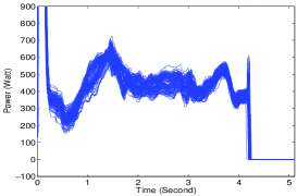
Figure 4: Time series of the switch operations (115 curves).

As we mentioned it in the introduction, the aim is to detect non-normal times series for a diagnosis prospective. An important preliminary task of this diagnosis task is the automatic identification of groups of switch operations having similar characteristics. For this purpose, we use the proposed EM algorithm for clustering these time series.

With this diagnosis specificity, we assume that the database is composed of two clusters, one corresponding to an operating state without defect and another corresponding to and operating state with a defect, that is $K=2$. The number of regression components of the proposed algorithm was set to $R=6$ in accordance with the number of electromechanical phases of a switch operation and the degree of the polynomial regression $p$ was set to 3 which is more appropriate for the different regimes in the time series.

IV-B2 Obtained results

Figure 5 shows the graphical clustering results and the corresponding clusters approximation for the time series of the real switch operation curves. Since the true class labels are unknown, we only consider the intra-class inertias which are given in Table III. It can be observed on Figure 5 that the time series of the first obtained cluster (middle) and the second one (right) does not have the same characteristics since their shapes are clearly different. Therefore they may correspond to two different stated of the switch mechanism. In particular, for the time series belonging to the first cluster (middle), it can be observed that something happened at around 4.2 Second of the switch operation. According to the experts, this can be attributed to a default in the measurement process. We note that the average running time of the EM algorithm for this experiment is about 40 S.

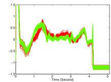
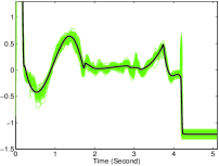
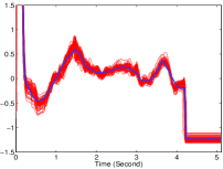
Figure 5: Clustering results for the switch operation time series obtained for $K=6$ and $p=3$.

$K$-means	EM for GMM	MixReg	MixHMM	MixHMMR
827.34	715.19	732.25	728.56	695.87

TABLE III: Intra-cluster inertia for the real data.

V Conclusion and future works

In this paper, we introduced a new model-based clustering approach for time series. The proposed model consists in a mixture of polynomial regression models governed by hidden Markov chains. The underlying Markov chain allows for successively activating various polynomial regression components over time. The model is therefore particularly appropriate for clustering times series with various changes in regime. The experimental results demonstrated the benefit of the proposed approach as compared to existing alternative methods, including the regression mixture model and the standard mixture of Hidden Markov Models. At this stage, we only gave the theoretical approach for selecting a model structure trough the BIC criterion. Current experiments are concerned with this problem and future works will discuss the problem of model selection.

References

- [1] A. P. Dempster, N. M. Laird, and D. B. Rubin, “Maximum likelihood from incomplete data via the EM algorithm,” Journal of The Royal Statistical Society, B, vol. 39(1), pp. 1–38, 1977.
- [2] G. M. James and C. Sugar, “Clustering for sparsely sampled functional data,” JASA, vol. 98, no. 462, 2003.
- [3] S. Gaffney and P. Smyth, “Trajectory clustering with mixtures of regression models,” in Proceedings of the fifth ACM SIGKDD. ACM Press, 1999, pp. 63–72.
- [4] S. J. Gaffney and P. Smyth, “Joint probabilistic curve clustering and alignment,” in In Advances in NIPS, 2004.
- [5] X. Liu and M. Yang, “Simultaneous curve registration and clustering for functional data,” CSDA, vol. 53, no. 4, pp. 1361–1376, 2009.
- [6] Y. Chi, X. Song, D. Zhou, K. Hino, and B. L. Tseng, “On evolutionary spectral clustering,” ACM Transactions on Knowledge Discovery from Data, vol. 3, no. 4, November 2009.
- [7] P. Smyth, “Clustering sequences with hidden markov models,” in Advances in NIPS 9, 1996, pp. 648–654.
- [8] S. J. Gaffney, “Probabilistic curve-aligned clustering and prediction with regression mixture models,” Ph.D. dissertation, Department of Computer Science, University of California, Irvine., 2004.
- [9] J. D. Banfield and A. E. Raftery, “Model-based gaussian and non-gaussian clustering,” Biometrics, vol. 49, no. 3, pp. 803–821, 1993.
- [10] G. McLachlan and K. Basford, Mixture Models: Inference and Applications to Clustering. Marcel Dekker, New York, 1988.
- [11] C. Fraley and A. E. Raftery, “Model-based clustering, discriminant analysis, and density estimation,” JASA, vol. 97, pp. 611–631, 2002.
- [12] G. J. McLachlan and D. Peel., Finite mixture models. New York: Wiley, 2000.
- [13] G. J. McLachlan and T. Krishnan, The EM algorithm and extensions. New York: Wiley, 1997.
- [14] L. R. Rabiner, “A tutorial on hidden markov models and selected applications in speech recognition,” Proceedings of the IEEE, vol. 77, no. 2, pp. 257–286, 1989.
- [15] L. Derrode, S. Benyoussef and W. Pieczynski, “Contextual estimation of hidden markov chains with application to image segmentation,” in ICASSP, Toulouse, May 2006, pp. 15–19.
- [16] J. Alon, S. Sclaroff, G. Kollios, and V. Pavlovic, “Discovering clusters in motion time-series data,” Los Alamitos, USA, 2003, pp. 375–381.
- [17] M. Fridman, “Hidden markov model regression,” Institute of mathematics, University of Minnesota, Tech. Rep., 1993.
- [18] L. Baum, T. Petrie, G. Soules, and N. Weiss, “A maximization technique occurring in the statistical analysis of probabilistic functions of markov chains,” Annals of Mathematical Statistics, vol. 41, pp. 164–171, 1970.
- [19] G. Schwarz, “Estimating the dimension of a model,” Annals of Statistics, vol. 6, pp. 461–464, 1978.