Effective Degrees of Freedom: A Flawed Metaphor

Abstract

To most applied statisticians, a fitting procedure’s degrees of freedom is synonymous with its model complexity, or its capacity for overfitting to data. In particular, it is often used to parameterize the bias-variance tradeoff in model selection. We argue that, contrary to folk intuition, model complexity and degrees of freedom are not synonymous and may correspond very poorly. We exhibit and theoretically explore various examples of fitting procedures for which degrees of freedom is not monotonic in the model complexity parameter, and can exceed the total dimension of the response space. Even in very simple settings, the degrees of freedom can exceed the dimension of the ambient space by an arbitrarily large amount. We show the degrees of freedom for any non-convex projection method can be unbounded.

1 Introduction

Consider observing data $\boldsymbol{y}=\boldsymbol{\mu}+\boldsymbol{\varepsilon}$ with fixed mean $\boldsymbol{\mu}\in\mathbb{R}^{n}$ and mean-zero errors $\boldsymbol{\varepsilon}\in\mathbb{R}^{n}$, and predicting $\boldsymbol{y}^{*}=\boldsymbol{\mu}+\boldsymbol{\varepsilon}^{*}$, where $\boldsymbol{\varepsilon}^{*}$ is an independent copy of $\boldsymbol{\varepsilon}$. Assume for simplicity the entries of $\boldsymbol{\varepsilon}^{*}$ and $\boldsymbol{\varepsilon}$ are independent and identically distributed with variance $\sigma^{2}$.

Statisticians have proposed an immense variety of fitting procedures for producing the prediction $\hat{\boldsymbol{y}}(\boldsymbol{y})$, some of which are more complex than others. The effective degrees of freedom (DF) of Efron, (1986), defined precisely as $\frac{1}{\sigma^{2}}\sum^{n}_{i=1}\operatorname{Cov}\big{(}y_{i},\hat{y}_{i}\big{)}$, has emerged as a popular and convenient measuring stick for comparing the complexity of very different fitting procedures (we motivate this definition in Section 2). The name suggests that a method with $p$ degrees of freedom is similarly complex as linear regression on $p$ predictor variables.

To motivate our inquiry, consider estimating a no-intercept linear regression model with design matrix $\boldsymbol{X}=\begin{pmatrix}1&0\\ 0&1\end{pmatrix}$ and response $\boldsymbol{y}\sim N(\boldsymbol{\mu},I)$, with $\boldsymbol{\mu}\in\mathbb{R}^{2}$. Suppose further that, in order to obtain a more parsimonious model than the full bivariate regression, we instead estimate the best fitting of the two univariate models (in other words, best subsets regression with model size $k=1$). In effect we are minimizing training error over the model $\boldsymbol{\mu}\in\mathcal{M}=\mathbb{R}\times\{0\}\cup\{0\}\times\mathbb{R}$. What are the effective degrees of freedom of the fitted model in this seemingly innocuous setting?

A simple, intuitive, and wrong argument predicts that the DF lies somewhere between 1 and 2. We expect it to be greater than 1, since we use the data to select the better of two one-dimensional models. However, we have only two free parameters at our disposal, with a rather severe constraint on the values they are allowed to take, so $\mathcal{M}$ is strictly less complex than the saturated model with two parameters that fits the data as hard as possible.

Figure 1 shows the effective DF for this model, plotted as a function of $\boldsymbol{\mu}\in\mathbb{R}^{2}$, the expectation of the response $\boldsymbol{y}$. As expected, $\text{DF}(\boldsymbol{\mu})\geq 1$, with near-equality when $\boldsymbol{\mu}$ is close to one of the coordinate axes but far from the other. Perhaps surprisingly, however, $\text{DF}(\boldsymbol{\mu})$ can exceed 2, approaching 7 in the corners of the plot. Indeed, the plot suggests (and we will later confirm) that $\text{DF}(\boldsymbol{\mu})$ can grow arbitrarily large as $\boldsymbol{\mu}$ moves farther diagonally from the origin.

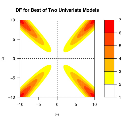
Figure 1: Heatmap of the DF for 1-best-subset fit with the model ${\boldsymbol{y}\sim N(I_{2}\cdot\boldsymbol{\beta},I_{2}\cdot\sigma^{2})}$, as a function of the true mean vector $\boldsymbol{\mu}\in\mathbb{R}^{2}$. Contrary to what one might naively expect, the DF can significantly exceed 2, the DF for the full model.

To understand why our intuition should lead us astray here, we must first review how the DF is defined for a general fitting procedure, and what classical concept that definition is meant to generalize.

1.1 Degrees of Freedom in Classical Statistics

The original meaning of degrees of freedom, the number of dimensions in which a random vector may vary, plays a central role in classical statistics. In ordinary linear regression with full-rank $n\times p$ predictor matrix $\boldsymbol{X}$, the fitted response $\hat{\boldsymbol{y}}=\boldsymbol{X}\hat{\boldsymbol{\beta}}$ is the orthogonal projection of $\boldsymbol{y}$ onto the $p$-dimensional column space of $\boldsymbol{X}$, and the residual $\boldsymbol{r}=\boldsymbol{y}-\hat{\boldsymbol{y}}$ is the projection onto its orthogonal complement, whose dimension is $n-p$. We say this linear model has $p$ “model degrees of freedom” (or just “degrees of freedom”), with $n-p$ “residual degrees of freedom.”

If the error variance is $\sigma^{2}$, then $\boldsymbol{r}$ is “pinned down” to have zero projection in $p$ directions, and is free to vary, with variance $\sigma^{2}$, in the remaining $n-p$ orthogonal directions. In particular, if the model is correct ($\mathbb{E}[\boldsymbol{y}]=\boldsymbol{X}\boldsymbol{\beta}$), then the residual sum of squares (RSS) has distribution

$$\text{RSS}=\|\boldsymbol{r}\|_{2}^{2}\sim\sigma^{2}\cdot\chi_{n-p}^{2}.$$ (1)

It follows that $\mathbb{E}\left[\|\boldsymbol{r}\|_{2}^{2}\right]=\sigma^{2}(n-p)$, leading to the unbiased variance estimate $\hat{\sigma}^{2}=\frac{1}{n-p}\|\boldsymbol{r}\|_{2}^{2}$. $t$-tests and $F$-tests are based on comparing lengths of $n$-variate Gaussian random vectors after projecting onto appropriate linear subspaces.

In linear regression, the model degrees of freedom (henceforth DF) serves to quantify multiple related properties of the fitting procedure. The DF coincides with the number of non-redundant free parameters in the model, and thus constitutes a natural measure of model complexity or overfitting. In addition, the total variance of the fitted response $\hat{\boldsymbol{y}}$ is exactly $\sigma^{2}p$, which depends only on the number of linearly independent predictors and not on their size or correlation with each other.

The DF also quantifies optimism of the residual sum of squares as an estimate of out-of-sample prediction error. In linear regression, one can easily show that the RSS understates mean squared prediction error by $2\sigma^{2}p$ on average. Mallows, (1973) proposed exploiting this identity as a means of model selection, by computing ${\text{RSS}+2\sigma^{2}}p$, an unbiased estimate of prediction error, for several models, and selecting the model with the smallest estimated test error. Thus, the DF of each model contributes a sort of penalty for how hard that model is fitted to the data.

1.2 “Effective” or “Equivalent” Degrees of Freedom

For more general fitting procedures such as smoothing splines, generalized additive models, or ridge regression, the number of free parameters is often either undefined or an inappropriate measure of model complexity. Most such methods feature some tuning parameter modulating the fit’s complexity, but it is not clear a priori how to compare e.g. a Lasso with Lagrange parameter $\lambda=3$ to a local regression with window width $0.5$. When comparing different methods, or the same method with different tuning parameters, it can be quite useful to have some measure of complexity with a consistent meaning across a diverse range of algorithms. To this end, various authors have proposed alternative, more general definitions of a method’s “effective degrees of freedom,” or “equivalent degrees of freedom” (see Buja et al., (1989) and references therein).

If the method is linear — that is, if $\hat{\boldsymbol{y}}=\boldsymbol{H}\boldsymbol{y}$ for some “hat matrix” $\boldsymbol{H}$ that is not a function of $\boldsymbol{y}$ — then the trace of $\boldsymbol{H}$ serves as a natural generalization. For linear regression $\boldsymbol{H}$ is a $p$-dimensional projection, so $\operatorname{tr}(\boldsymbol{H})=p$, coinciding with the original definition. Intuitively, when $\boldsymbol{H}$ is not a projection, $\operatorname{tr}(\boldsymbol{H})$ accumulates fractional degrees of freedom for directions of $\boldsymbol{y}$ that are shrunk, but not entirely eliminated, in computing $\hat{\boldsymbol{y}}$.

For nonlinear methods, further generalization is necessary. The most popular definition, due to Efron, (1986) and given in Equation (4), defines DF in terms of the optimism of RSS as an estimate of test error, and applies to any fitting method.

Measuring or estimating optimism is a worthy goal in and of itself. But to justify our intuition that the DF offers a consistent way to quantify model complexity, a bare requirement is that the DF be monotone in model complexity when considering a fixed method.

The term “model complexity” is itself rather metaphorical when describing arbitrary fitting algorithms, but has a concrete meaning for methods that minimize RSS subject to the fit $\hat{\boldsymbol{y}}$ belonging to a closed constraint set $\mathcal{M}$ (a “model”). Commonly, some tuning parameter $\gamma$ selects one of a nested set of models:

$$\hat{\boldsymbol{y}}^{(\gamma)}=\operatorname*{arg\,min}_{\boldsymbol{z}\in\mathcal{M}_{\gamma}}\|\boldsymbol{y}-\boldsymbol{z}\|_{2}^{2},\;\;\;\text{ with }\mathcal{M}_{\gamma_{1}}\subseteq\mathcal{M}_{\gamma_{2}}\subseteq\mathbb{R}^{n}\text{ if }\gamma_{1}\leq\gamma_{2}$$ (2)

Examples include the Lasso (Tibshirani,, 1996) and ridge regression (Hoerl,, 1962) in their constraint formulation, as well as best subsets regression (BSR). The model $\mathcal{M}_{k}$ for BSR with $k$ variables is a union of $k$-dimensional subspaces.

Because larger models “fit harder” to the data, one naturally expects DF to be monotone with respect to model inclusion. For example, one might imagine a plot of DF versus $k$ for BSR to look like Figure 2 when the full model has $p=10$ predictors: monotone and sandwiched between $k$ and $p$.

Figure 2: This plot follows the usual intuition for degrees of freedom for best subset regression when the full model has 10 predictors.

However, as we have already seen in Figure 1, monotonicity is far from guaranteed even in very simple examples, and in particular the DF “ceiling” at $p$ can be broken. Surprisingly, monotonicity can even break down for methods projecting onto convex sets, including ridge regression and the Lasso (although the DF cannot exceed the dimension of the convex set). The non-monotonicity of DF for such convex methods was discovered independently by Kaufman and Rosset, (2014), who give a thorough account. Among other results, they prove that the degrees of freedom of projection onto any convex set must always be smaller than the dimension of that set.

To minimize overlap with Kaufman and Rosset, (2014), we focus our attention instead on non-convex fitting procedures such as BSR. In contrast to the results of Kaufman and Rosset, (2014) for the convex case, we show that projection onto any closed non-convex set can have arbitrarily large degrees of freedom, regardless of the dimensions of $\mathcal{M}$ and $\boldsymbol{y}$.

2 Preliminaries

We consider fitting techniques with some tuning parameter (discrete or continuous) that can be used to vary the model from less to more constrained. In BSR, the tuning parameter $k$ determines how many predictor variables are retained in the model, and we will denote BSR with tuning parameter $k$ as BSR_k. For a general fitting technique FIT, we will use the notation FIT_k for FIT with tuning parameter $k$ and $\hat{\boldsymbol{y}}^{{\scriptscriptstyle(FIT_{k})}}$ for the fitted response produced by FIT_k.

As mentioned in the introduction, a general formula for DF can be motivated by the following relationship between expected prediction error (EPE) and RSS for ordinary least squares (OLS) (Mallows,, 1973):

$$\text{EPE}=\mathbb{E}[\text{RSS}]+2\sigma^{2}p.$$ (3)

Analogously, once a fitting technique (and tuning parameter) FIT_k is chosen for fixed data $\boldsymbol{y}$, DF is defined by the following identity:

$$\mathbb{E}\left[\sum^{n}_{i=1}(y^{*}_{i}-\hat{y}^{{\scriptscriptstyle(FIT_{k})}}_{i})^{2}\right]=\mathbb{E}\left[\sum^{n}_{i=1}(y_{i}-\hat{y}^{{\scriptscriptstyle(FIT_{k})}}_{i})^{2}\right]+2\sigma^{2}\cdot\text{DF}(\boldsymbol{\mu},\sigma^{2},\text{FIT}_{k}),$$ (4)

where $\sigma^{2}$ is the variance of the $\varepsilon_{i}$ (which we assume exists), and $y^{*}_{i}$ is a new independent copy of $y_{i}$ with mean $\boldsymbol{\mu}_{i}$. Thus DF is defined as a measure of the optimism of RSS. This definition in turn leads to a simple closed form expression for DF under very general conditions, as shown by the following theorem.

Theorem 1 (Efron, (1986)).

For $i\in\{1,\dots,n\}$, let $y_{i}=\mu_{i}+\varepsilon_{i}$, where the $\mu_{i}$ are nonrandom and the $\varepsilon_{i}$ have mean zero and finite variance. Let $\hat{y}_{i},\;i\in\{1,\dots,n\}$ denote estimates of $\mu_{i}$ from some fitting technique based on a fixed realization of the $y_{i}$, and let $y^{*}_{i},\;i\in\{1,\dots,n\}$ be independent of and identically distributed as the $y_{i}$. Then

$$\mathbb{E}\left[\sum^{n}_{i=1}(y^{*}_{i}-\hat{y}_{i})^{2}\right]-\mathbb{E}\left[\sum^{n}_{i=1}(y_{i}-\hat{y}_{i})^{2}\right]=2\sum^{n}_{i=1}\operatorname{Cov}(y_{i},\hat{y}_{i})$$ (5)

Proof.

For $i\in\{1,\dots,n\}$,

$$\begin{split}\mathbb{E}\big{[}(y^{*}_{i}-\hat{y}_{i})^{2}\big{]}&=\mathbb{E}\big{[}(y^{*}_{i}-\mu_{i}+\mu_{i}-\hat{y}_{i})^{2}\big{]}\\ &=\mathbb{E}\big{[}(y^{*}_{i}-\mu_{i})^{2}\big{]}+2\mathbb{E}\big{[}(y^{*}_{i}-\mu_{i})(\mu_{i}-\hat{y}_{i})\big{]}+\mathbb{E}\big{[}(\mu_{i}-\hat{y}_{i})^{2}\big{]}\\ &=\operatorname{Var}(\varepsilon_{i})+\mathbb{E}\big{[}(\mu_{i}-\hat{y}_{i})^{2}\big{]},\end{split}$$ (6)

where the middle term in the second line equals zero because $y^{*}_{i}$ is independent of all the $y_{j}$ and thus also of $\hat{y}_{i}$, and because $\mathbb{E}\big{[}y^{*}_{i}-\mu_{i}\big{]}=0$. Furthermore,

$$\begin{split}\mathbb{E}\big{[}(y_{i}-\hat{y}_{i})^{2}\big{]}&=\mathbb{E}\big{[}(y_{i}-\mu_{i}+\mu_{i}-\hat{y}_{i})^{2}\big{]}\\ &=\mathbb{E}\big{[}(y_{i}-\mu_{i})^{2}\big{]}+2\mathbb{E}\big{[}(y_{i}-\mu_{i})(\mu_{i}-\hat{y}_{i})\big{]}+\mathbb{E}\big{[}(\mu_{i}-\hat{y}_{i})^{2}\big{]}\\ &=\operatorname{Var}(\varepsilon_{i})+\mathbb{E}\big{[}(\mu_{i}-\hat{y}_{i})^{2}\big{]}-2\operatorname{Cov}(y_{i},\hat{y}_{i}).\end{split}$$ (7)

Finally, subtracting Equation (7) from Equation (6) and summing over ${i\in\{1,\dots,n\}}$ gives the desired result. ∎

Remark 1.

For i.i.d. errors with finite variance $\sigma^{2}$, Theorem 1 implies that,

$$\text{DF}(\boldsymbol{\mu},\sigma^{2},\text{FIT}_{k})=\frac{1}{\sigma^{2}}\operatorname{tr}\big{(}\operatorname{Cov}(\boldsymbol{y},\hat{\boldsymbol{y}}^{{\scriptscriptstyle(FIT_{k})}})\big{)}=\frac{1}{\sigma^{2}}\sum^{n}_{i=1}\operatorname{Cov}\big{(}y_{i},\hat{y}^{{\scriptscriptstyle(FIT_{k})}}_{i}\big{)}.$$ (8)

Note also that when FIT_k is a linear fitting method with hat matrix $\boldsymbol{H}$, Equation (8) reduces to

$$\text{DF}(\boldsymbol{\mu},\sigma^{2},\text{FIT}_{k})=\operatorname{tr}(\boldsymbol{H}).$$ (9)

3 Additional Examples

For each of the following examples, a model-fitting technique, mean vector, and noise process are chosen. Then the DF is estimated by Monte Carlo simulation. The details of this estimation process, along with all R code used, are provided in the appendix.

3.1 Best Subset Regression Example

Our first motivating example is meant to mimic a realistic application. This example is a linear model with $n=50$ observations on $p=15$ variables and a standard Gaussian noise process. The design matrix $\boldsymbol{X}$ is a $n\times p$ matrix of i.i.d. standard Gaussian noise. The mean vector $\boldsymbol{\mu}$ (or equivalently, the coefficient vector $\boldsymbol{\beta}$) is generated by initially setting the coefficient vector to the vector of ones, and then standardizing $\boldsymbol{X}\boldsymbol{\beta}$ to have mean zero and standard deviation seven. We generated a few $(\boldsymbol{X},\boldsymbol{\beta})$ pairs before we discovered one with substantially non-monotonic DF, but then measured the DF for that $(\boldsymbol{X},\boldsymbol{\beta})$ to high precision via Monte Carlo.

Figure 3: Monte Carlo estimated degrees of freedom versus subset size in the best subset regression (left) and forward stepwise regression (right) examples. Estimates are shown plus or minus two (Monte Carlo) standard errors. Dashed lines show the constant ambient dimension ($p$) and the increasing subset size, for reference ($k$).

The left plot of Figure 3 shows the plot of Monte Carlo estimated DF versus subset size. The right plot of Figure 3 shows the same plot for forward stepwise regression (FSR) applied to the same data. Although FSR isn’t quite a constrained least-squares fitting method, it is a popular method whose complexity is clearly increasing in $k$. Both plots show that the DF for a number of subset sizes is greater than 15, and we know from standard OLS theory that the DF for subset size 15 is exactly 15 in both cases.

3.2 Unbounded Degrees of Freedom Example

Next we return to the motivating example from Section 1. The setup is again a linear model, but with $n=p=2$. The design matrix $\boldsymbol{X}=A\cdot\boldsymbol{I}$, where $A$ is a scalar and $\boldsymbol{I}$ is the ($2\times 2$) identity matrix. The coefficient vector is just $(1,1)^{T}$ making the mean vector $(A,A)^{T}$, and the noise is i.i.d. standard Gaussian. Considering BSR₁, with high probability for large $A$ (when $\boldsymbol{y}$ falls in the positive quadrant), it is clear that the best univariate model just chooses the larger of the two response variables for each realization. Simulating $10^{5}$ times with $A=10^{4}$, we get a Monte Carlo estimate of the DF of BSR₁ to be about 5630, with a standard error of about 26. Playing with the value of $A$ reveals that for large $A$, DF is approximately linearly increasing in $A$. This suggests that not only is the DF greater than $n=2$, but can be made unbounded without changing $n$ or the structure of $\boldsymbol{X}$. Figure 4 shows what is going on for a few points (and a smaller value of $A$ for visual clarity). The variance of the $y_{i}$ (the black points) is far smaller than that of the $\hat{y}_{i}$ (the projections of the black dots onto the blue constraint set). Therefore, since the correlation between the $y_{i}$ and the $\hat{y}_{i}$ is around 0.5, $\sum_{i=1}^{n}\operatorname{Cov}(y_{i},\hat{y}_{i})$ is also much larger than the variance of the $y_{i}$, and the large DF can be infered from Equation (8).

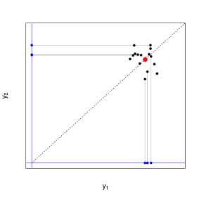
Figure 4: Sketch of the unbounded DF example (not to scale with the $A$ value used in the text). The true mean vector is in red, the constraint region in blue, and some data points are shown in black. The grey lines connect some of the data points to their projections onto the constraint set, in blue. Note that for ${i\in\{1,2\}}$, $\hat{\boldsymbol{y}}_{i}$ is either 0 or approximately $A$ depending on small changes in $\boldsymbol{y}$.

In this toy example, we can actually prove that the DF diverges as $A\rightarrow\infty$ using Equation (4),

$$\begin{split}\frac{1}{A}\text{DF}((A,A)^{T},1,\text{BSR}_{1})&=\frac{1}{2}\mathbb{E}\left[\frac{1}{A}\sum^{2}_{i=1}\Big{(}(y^{*}_{i}-\hat{y}^{{\scriptscriptstyle(BSR_{1})}}_{i})^{2}-(y_{i}-\hat{y}^{{\scriptscriptstyle(BSR_{1})}}_{i})^{2}\Big{)}\right]\\ &=\frac{1}{2}\mathbb{E}\left[\frac{1}{A}\sum^{2}_{i=1}\Big{(}(y^{*}_{i}-\hat{y}^{{\scriptscriptstyle(BSR_{1})}}_{i})^{2}-(y_{i}-\hat{y}^{{\scriptscriptstyle(BSR_{1})}}_{i})^{2}\Big{)}\mathbb{I}_{\boldsymbol{y}\in Q_{1}}\right]\\ &\quad+\frac{1}{2}\mathbb{E}\left[\frac{1}{A}\sum^{2}_{i=1}\Big{(}(y^{*}_{i}-\hat{y}^{{\scriptscriptstyle(BSR_{1})}}_{i})^{2}-(y_{i}-\hat{y}^{{\scriptscriptstyle(BSR_{1})}}_{i})^{2}\Big{)}\mathbb{I}_{\boldsymbol{y}\notin Q_{1}}\right]\\ &=\frac{1}{2}\mathbb{E}\left[\frac{1}{A}\Big{(}A^{2}+2A\varepsilon_{1}^{*}+(\varepsilon_{1}^{*})^{2}+\big{(}\varepsilon_{2}^{*}-\min(\varepsilon_{1},\varepsilon_{2})\big{)}^{2}\right.\\ &\quad\qquad\qquad\left.-A^{2}-2A\min(\varepsilon_{1},\varepsilon_{2})-\big{(}\min(\varepsilon_{1},\varepsilon_{2})\big{)}^{2}\Big{)}\mathbb{I}_{\boldsymbol{y}\in Q_{1}}\right]\\ &\quad+o(1)\\ &\stackrel{{\scriptstyle A\rightarrow\infty}}{{\longrightarrow}}\frac{1}{2}\mathbb{E}\left[2\varepsilon_{1}^{*}-2\min(\varepsilon_{1},\varepsilon_{2})\right]=\mathbb{E}\left[\max(\varepsilon_{1},\varepsilon_{2})\right],\\ \end{split}$$ (10)

where $Q_{1}$ is the first quadrant of $\mathbb{R}^{2}$, $\mathbb{I}_{S}$ is the indicator function on the set $S$, and $\varepsilon_{1}^{*},\varepsilon_{2}^{*}$ are noise realizations independent of one another and of $\boldsymbol{y}$. The $o(1)$ term comes from the the fact that $\frac{1}{A}\sum^{2}_{i=1}\Big{(}(y^{*}_{i}-\hat{y}^{{\scriptscriptstyle(BSR_{1})}}_{i})^{2}-(y_{i}-\hat{y}^{{\scriptscriptstyle(BSR_{1})}}_{i})^{2}\Big{)}$ is $O_{p}(A)$ while $\mathbb{P}(\boldsymbol{y}\notin Q)$ shrinks exponentially fast in $A$ (as it is a Gaussian tail probability). The convergence in the last line follows by the Dominated Convergence Theorem applied to the first term in the preceding line. Note that $\mathbb{E}\left[\max(\varepsilon_{1},\varepsilon_{2})\right]\approx 0.5642$, in good agreement with the simulated result.

4 Geometric Picture

The explanation for the non-monotonicity of DF can be best understood by thinking about regression problems as constrained optimizations. We will see that the reversal in DF monotonicity is caused by the interplay between the shape of the coefficient constraint set and that of the contours of the objective function.

BSR has a non-convex constraint set for $k<p$, and Subsection 3.2 gives some intuition for why the DF can be much greater than the model dimension. This intuition can be generalized to any non-convex constraint set, as follows. Place the true mean at a point with non-unique projection onto the constraint set, see Figure 5 for a generic sketch. Such a point must exist by the Motzkin-Bunt Theorem (Bunt,, 1934; Motzkin,, 1935; Kritikos,, 1938). Note the constraint set for $\hat{\boldsymbol{y}}=\boldsymbol{X}\hat{\boldsymbol{\beta}}$ is just an affine transformation of the constraint set for $\hat{\boldsymbol{\beta}}$, and thus a non-convex $\hat{\boldsymbol{\beta}}$ constraint is equivalent to a non-convex $\hat{\boldsymbol{y}}$ constraint. Then the fit depends sensitively on the noise process, even when the noise is very small, since $\boldsymbol{y}$ is projected onto multiple well-separated sections of the constraint set. Thus as the magnitude of the noise, $\sigma$, goes to zero, the variance of $\hat{\boldsymbol{y}}$ remains roughly constant. Equation (8) then tells us that DF can be made arbitrarily large, as it will be roughly proportional to $\sigma^{-1}$. We formalize this intuition in the following theorem.

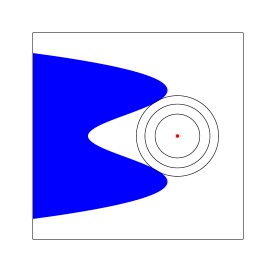
Figure 5: Sketch of geometric picture for a regression problem with $n=2$ and non-convex constraint sets. The blue area is the constraint set, the red point the true mean vector, and the black circles the contours of the least squares objective function. Note how the spherical contour spans the gap of the divot where it meets the constraint set.

Theorem 2.

For a fitting technique FIT that minimizes squared error subject to a non-convex, closed constraint $\hat{\boldsymbol{\mu}}\in\mathcal{M}\subset\mathbb{R}^{n}$, consider the model,

$$\boldsymbol{y}=\boldsymbol{\mu}+\sigma\boldsymbol{\varepsilon},\quad\varepsilon_{i}\stackrel{{\scriptstyle\emph{i.i.d.}}}{{\sim}}F\text{ for }i\in\{1,\dots,n\},$$

where $F$ is a mean-zero distribution with finite variance supported on an open neighborhood of 0. Then there exists some $\boldsymbol{\mu}^{*}$ such that $\text{DF}(\boldsymbol{\mu}^{*},\sigma^{2},\text{FIT}_{k})\rightarrow\infty$ as $\sigma^{2}\rightarrow 0$.

Proof.

We leave the proof for the appendix. ∎

5 Discussion

The common intuition that “effective” or “equivalent” degrees of freedom serves a consistent and interpretable measure of model complexity merits some degree of skepticism. Our results and examples, combined with those of Kaufman and Rosset, (2014), demonstrate that for many widely-used convex and non-convex fitting techniques, the DF can be non-monotone with respect to model nesting. In the non-convex case, the DF can exceed the dimension of the model space by an arbitrarily large amount. This phenomenon is not restricted to pathological examples or edge cases, but can arise in run-of-the-mill datasets as well. Finally, we presented a geometric interpretation of this phenomenon in terms of irregularities in the model constraints and/or objective function contours.

In light of the above, we find the term “(effective) degrees of freedom” to be somewhat misleading, as it is suggestive of a quantity corresponding to model “size”. It is also misleading to consider DF as a measure of overfitting, or how flexibly the model is conforming to the data, since a model always fits at least as strongly as a strict submodel to a given dataset. By definition, the DF of Efron, (1983) does measure optimism of in-sample error as an estimate of out-of-sample error, but we should not be too quick to assume that our intuition about linear models carries over exactly.

6 Appendix A

Proof of Theorem 2.

The proof relies heavily on the fact that for every non-convex set $\cal M$ in Euclidean space there is at least one point whose projection onto $\cal M$ is not unique (e.g. the red dot in Figure 5). This fact was proved independently in Bunt, (1934), Motzkin, (1935), and Kritikos, (1938). A schematic for this proof in two dimensions is provided in Figure 6.

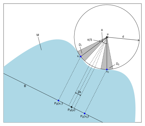
Figure 6: Schematic for the proof of Theorem 2, in two dimensions.

Let $\boldsymbol{\mu}$ be a point with non-unique projection onto the non-convex set $\mathcal{M}$ and let $\boldsymbol{x}_{1}$ and $\boldsymbol{x}_{2}$ be two distinct projections of $\boldsymbol{\mu}$ onto $\mathcal{M}$. Let $d=||\boldsymbol{\mu}-\boldsymbol{x}_{1}||_{2}=||\boldsymbol{\mu}-\boldsymbol{x}_{2}||_{2}$ be the Euclidean distance between $\boldsymbol{\mu}$ and $\mathcal{M}$, and $\theta=\cos^{-1}(\frac{(\boldsymbol{x}_{1}-\boldsymbol{\mu})\cdot(\boldsymbol{x}_{2}-\boldsymbol{\mu})}{|\boldsymbol{x}_{1}-\boldsymbol{\mu}||\boldsymbol{x}_{2}-\boldsymbol{\mu}|})$ be the angle between $\boldsymbol{x}_{1}$ and $\boldsymbol{x}_{2}$, taken as vectors from $\boldsymbol{\mu}$. Define the set $\mathcal{D}_{1}=\{\boldsymbol{v}\in\mathbb{R}^{n}|\cos^{-1}(\frac{(\boldsymbol{x}_{1}-\boldsymbol{\mu})\cdot(\boldsymbol{v}-\boldsymbol{\mu})}{|\boldsymbol{x}_{1}-\boldsymbol{\mu}||\boldsymbol{v}-\boldsymbol{\mu}|})<\frac{\theta}{5},||\boldsymbol{v}-\boldsymbol{\mu}||_{2}<d\}$, and $\mathcal{D}_{2}$ analogously for $\boldsymbol{x}_{2}$. Let $\mathcal{B}$ be a one-dimensional affine subspace that is both parallel to the line connecting $\boldsymbol{x}_{1}$ and $\boldsymbol{x}_{2}$, and contained in the hyperplane defined by $\boldsymbol{\mu}$, $\boldsymbol{x}_{1}$, and $\boldsymbol{x}_{2}$. Denoting the projection operator onto $\mathcal{B}$ by $P_{\mathcal{B}}$, let $z=||P_{\mathcal{B}}\boldsymbol{y}-P_{\mathcal{B}}\boldsymbol{\mu}||_{2}/\sigma$, and $\tilde{y}=||P_{\mathcal{B}}\hat{\boldsymbol{y}}-P_{\mathcal{B}}\boldsymbol{\mu}||_{2}$. Let $a=d\cos(\frac{\pi-\theta/5}{2})$. We now have,

$$\begin{split}\operatorname{tr}(\operatorname{Cov}(\boldsymbol{y},\hat{\boldsymbol{y}}))&\geq\operatorname{Cov}(P_{\mathcal{B}}\boldsymbol{y},P_{\mathcal{B}}\hat{\boldsymbol{y}})\\ &=\mathbb{E}[\sigma z\tilde{y}]\\ &=\mathbb{E}[\sigma z\tilde{y}1_{y\in\mathcal{D}_{1}\cup\mathcal{D}_{2}}]+\mathbb{E}[\sigma z\tilde{y}1_{y\notin\mathcal{D}_{1}\cup\mathcal{D}_{2}}]\\ &\geq\sigma\mathbb{E}[z\tilde{y}1_{y\in\mathcal{D}_{1}}]+\sigma\mathbb{E}[z\tilde{y}1_{y\in\mathcal{D}_{2}}]\\ &\geq a\sigma\big{(}\mathbb{E}[z1_{y\in\mathcal{D}_{2}}]-\mathbb{E}[z1_{y\in\mathcal{D}_{1}}]\big{)},\\ &=2a\sigma\mathbb{E}[z1_{y\in\mathcal{D}_{2}}].\\ \end{split}$$

The first inequality follows from the translation and rotation invariance of the trace of a covariance matrix, and from the positivity of the diagonal entries of the covariance matrix for the case of projection fitting methods. For the second inequality, note that $\mathbb{E}[\sigma z\tilde{y}1_{y\notin\mathcal{D}_{1}\cup\mathcal{D}_{2}}]\geq 0$, again because of the positivity of the DF of projection methods (applied to the same model with a noise process that has support on $\mathcal{D}_{1}$ and $\mathcal{D}_{2}$ removed). The third inequality follows from considering the projections of $\mathcal{D}_{1}$ and $\mathcal{D}_{2}$ onto $\mathcal{M}$ and then onto $\mathcal{B}$, and noting that the two (double) projections must be separated by at least a distance of $2a$.

Defining $\mathcal{F}_{1}=\{\boldsymbol{v}\in\mathbb{R}^{n}|\cos^{-1}(\frac{(\boldsymbol{x}_{1}-\boldsymbol{\mu})\cdot(\boldsymbol{v}-\boldsymbol{\mu})}{|\boldsymbol{x}_{1}-\boldsymbol{\mu}||\boldsymbol{v}-\boldsymbol{\mu}|})<\frac{\theta}{5}\}$ and $\mathcal{F}_{2}$ analogously for $\boldsymbol{x}_{2}$, note that $\mathbb{P}(\boldsymbol{y}\in\mathcal{F}_{1}\setminus\mathcal{D}_{1})=\mathbb{P}(\boldsymbol{y}\in\mathcal{F}_{2}\setminus\mathcal{D}_{2})\rightarrow 0$ as $\sigma^{2}\rightarrow 0$. Thus,

$$\begin{split}\operatorname{tr}(\operatorname{Cov}(\boldsymbol{y},\hat{\boldsymbol{y}}))&\geq 2a\sigma\big{(}\mathbb{E}[z1_{y\in\mathcal{F}_{2}}]+o(\sigma)\big{)}.\\ \end{split}$$

Neither $z$ nor the event $y\in\mathcal{F}_{2}$ depend on $\sigma$, so define the constant $b=2a\mathbb{E}[z1_{y\in\mathcal{F}_{2}}]>0$ which is independent of $\sigma$. Thus we have shown that,

$$\begin{split}\text{DF}(\boldsymbol{\mu}^{*},\sigma^{2},\text{FIT}_{k})&=\frac{1}{\sigma^{2}}\operatorname{tr}(\operatorname{Cov}(\boldsymbol{y},\hat{\boldsymbol{y}}))\\ &\geq\frac{b+o(\sigma)}{\sigma}\\ &\rightarrow\infty\end{split}$$

as $\sigma^{2}\rightarrow 0$. ∎

7 Appendix B

In Subsections 3.1 and 3.2, DF is estimated by computing an ubiased estimator of DF for each simulated noise realization. This unbiased estimator for DF can be obtained from Equation (8) by exploiting the linearity of the expectation and trace operators,

$$\begin{split}\text{DF}(\boldsymbol{\mu},\sigma^{2},\text{FIT}_{k})&=\frac{1}{\sigma^{2}}\operatorname{tr}(\operatorname{Cov}(\boldsymbol{y},\hat{\boldsymbol{y}}^{{\scriptscriptstyle(FIT_{k})}}))\\ &=\frac{1}{\sigma^{2}}\mathbb{E}\big{[}(\boldsymbol{y}-\boldsymbol{\mu})^{T}(\hat{\boldsymbol{y}}^{{\scriptscriptstyle(FIT_{k})}}-\mathbb{E}[\hat{\boldsymbol{y}}^{{\scriptscriptstyle(FIT_{k})}}])\big{]}\\ &=\frac{1}{\sigma^{2}}\mathbb{E}\big{[}\boldsymbol{\varepsilon}^{T}\hat{\boldsymbol{y}}^{{\scriptscriptstyle(FIT_{k})}}\big{]},\end{split}$$ (11)

where the last inequality follows because $\mathbb{E}[\boldsymbol{\varepsilon}]=\boldsymbol{0}$. Thus the true DF is estimated by $\boldsymbol{\varepsilon}^{T}\hat{\boldsymbol{y}}^{{\scriptscriptstyle(FIT_{k})}}$ averaged over many simulations. Since this estimate of DF is an average of i.i.d. random variables, its standard deviation can be estimated by the emipirical standard deviation of the $\boldsymbol{\varepsilon}^{T}\hat{\boldsymbol{y}}^{{\scriptscriptstyle(FIT_{k})}}$ divided by the square root of the number of simulations.

The following is the code for the BSR simulation in Subsection 3.1. Note that although the seed is preset, this is only done to generate a suitable design matrix, not to cherry-pick the simulated noise processes. The simulation results remain the same if the seed is reset after assigning the value to x.

⬇

library(leaps)

library(gplots)

n = 50; p = 15; B = 5000

set.seed(1113)

x = matrix(rnorm(n * p), n, p)

mu = drop(scale((x %*% rep(1, 15))))

snr = 7

mu = mu * snr

dfmat = matrix(0, B, p)

for(j in 1:B){

y = rnorm(n) + mu

#temp = regsubsets(x, y, nbest = 1, nvmax = p)

temp = regsubsets(x, y, nbest = 1, nvmax = p, intercept = FALSE)

for(i in 1:p){

jcoef = coef(temp, id = i)

#xnames = names(jcoef)[-1]

xnames = names(jcoef)

which = match(xnames, letters[1:p])

#yhat = cbind(1, x[ , which]) %*% jcoef

if(i == 1){

yhat = matrix(x[ , which], n, 1) %*% jcoef

} else{

yhat = x[ , which] %*% jcoef

}

dfmat[j, i] = sum((y - mu) * yhat)

}

}

#df = apply(dfmat, 2, mean) - 1

df = apply(dfmat, 2, mean)

error = sqrt(apply(dfmat, 2, var) / B)

save(df, error, p, file = "BSR.rdata")

plotCI(1:p, df, 2 * error, ylim = c(0, 35), xlim = c(0, p), gap = 0.4, xlab = "Subset Size", ylab = "Degrees of Freedom", cex.lab = 1.5, type = "o")

abline(h = 15, lty = 2)

lines(c(0, 15), c(0, 15), lty = 2)

title("Best Subset Regression", cex.main = 2)

The code for the FSR simulation in Subsection 3.1 is almost identical.

⬇

library(leaps)

library(gplots)

n = 50; p = 15; B = 5000

set.seed(1113)

x = matrix(rnorm(n * p), n, p)

mu = drop(scale((x %*% rep(1, 15))))

snr = 7

mu = mu * snr

dfmat = matrix(0, B, p)

for(j in 1:B){

y = rnorm(n) + mu

#temp = regsubsets(x, y, nbest = 1, nvmax = p, method = "forward")

temp = regsubsets(x, y, nbest = 1, nvmax = p, method = "forward", intercept = FALSE)

for(i in 1:p){

jcoef = coef(temp, id = i)

#xnames = names(jcoef)[-1]

xnames = names(jcoef)

which = match(xnames, letters[1:p])

#yhat = cbind(1, x[ , which]) %*% jcoef

if(i == 1){

yhat = matrix(x[ , which], n, 1) %*% jcoef

} else{

yhat = x[ , which] %*% jcoef

}

dfmat[j, i] = sum((y - mu) * yhat)

}

}

#df = apply(dfmat, 2, mean) - 1

df = apply(dfmat, 2, mean)

error = sqrt(apply(dfmat, 2, var) / B)

save(df, error, p, file = "FSR.rdata")

plotCI(1:p, df, 2 * error, ylim = c(0, 35), xlim = c(0, p), gap = 0.4, xlab = "Subset Size", ylab = "Degrees of Freedom", cex.lab = 1.5, type = "o")

abline(h = 15, lty = 2)

lines(c(0, 15), c(0, 15), lty = 2)

title("Forward Stepwise Regression", cex.main = 2)

Finally, the code for Subsection 3.2 is different but short. We can imagine taking $A\rightarrow\infty$.

⬇

# A is some big number

A = 10000

X = A * data.frame(diag(2))

B = 1E5

y = A + matrix(rnorm(2 * B), ncol = 2)

# best univariate (no-intercept) model just picks the larger y_i

yhat.bs = t(apply(y, MARGIN = 1, FUN = function(yy) yy * (yy > mean(yy))))

dfvec = drop(((y - A) * yhat.bs) %*% c(1, 1))

df = mean(dfvec)

error = sqrt(var(dfvec) / B)

c(df, error)

References

- Buja et al., (1989) Buja, A., Hastie, T., and Tibshirani, R. (1989). Linear smoothers and additive models. The Annals of Statistics, 17(2):453–510.
- Bunt, (1934) Bunt, L. N. H. (1934). Bijdrage tot de theorie der convexe puntverzamelingen. PhD thesis, Rijks-Universiteit, Groningen.
- Efron, (1983) Efron, B. (1983). Estimating the error rate of a prediction rule: improvement on cross-validation. Journal of the American Statistical Association, 78(382):316–331.
- Efron, (1986) Efron, B. (1986). How Biased Is the Apparent Error Rate of a Prediction Rule? Journal of the American Statistical Association, 81(394):461–470.
- Hoerl, (1962) Hoerl, A. E. (1962). Application of Ridge Analysis to Regression Problems. Chemical Engineering Progress, 58:54–59.
- Kaufman and Rosset, (2014) Kaufman, S. and Rosset, S. (2014). When Does More Regularization Imply Fewer Degrees of Freedom? Sufficient Conditions and Counter Examples from Lasso and Ridge Regression. Biometrika (to appear).
- Kritikos, (1938) Kritikos, M. N. (1938). Sur quelques propriétés des ensembles convexes. Bulletin Mathématique de la Société Roumaine des Sciences, 40:87–92.
- Mallows, (1973) Mallows, C. L. (1973). Some Comments on CP. Technometrics, 15(4):661–675.
- Motzkin, (1935) Motzkin, T. (1935). Sur quelques propriétés caractéristiques des ensembles convexes. Atti Accad. Naz. Lincei Rend. Cl. Sci. Fis. Mat. Natur, 21:562–567.
- Tibshirani, (1996) Tibshirani, R. (1996). Regression shrinkage and selection via the lasso. Journal of the Royal Statistical Society. Series B, 58(1):267–288.